A Semi-Supervised Machine Learning Model to Forecast Movements of Moored Vessels

Abstract

The good performance of the port activities in terminals is mainly conditioned by the dynamic response of the moored ship system at a berth. An adequate definition of the highly multivariate processes involved in the response of a moored ship at a berth is crucial for an appropriate characterization of port operability. The availability of an efficient forecast system of the movements of moored ships is essential for the planning, performance, and safety of the development of port operations. In this paper, an inference model to predict moored ship motions, based on a semi-supervised Machine Learning methodology, is presented. A comparison with different supervised and unsupervised Machine Learning techniques, as well as with existing Deep Learning-based models for predicting moored ship motions, has been performed. The highest performance of the semi-supervised Machine Learning-based model has been obtained. Additionally, the influence of infragravity wave parameters introduced as predictor variables in the model has been analyzed and compared with the typical ocean waves, wind, and sea level as predictor variables. The prediction model has been developed and validated with an available dataset of measured data from field campaigns in the Outer Port of Punta Langosteira (A Coruña, Spain).

1. Introduction

The efficient development of port operations (e.g., goods loading/unloading and passenger embarking/disembarking) is essential for the proper functioning of a harbor.

A good performance of a port’s activities is mainly conditioned by the dynamic response of the moored ship system (composed of a ship, mooring lines, and fenders) in a berthing area due to the met-ocean conditions (waves, wind, currents, and sea level). In this sense, the port operability can be limited because of the effect of certain unfavorable conditions driving excessive moored ship motions and even inducing downtime events. Traditionally, the port operability/downtime assessment is based on recommended exceedance thresholds of certain met-ocean and/or ship motion parameters [1,2,3,4,5,6,7,8,9]. Those limiting thresholds are defined as the maximum admissible values for the relevant variables in terms of the operational, functional, and safety conditions in the development of port operations. Different operability criteria defining the allowable moored ship motions for each of the six degrees of freedom (6 DoF) and different types of ship can be found in [2,3,4,5,6,7,8]. As an indirect measure of the induced responses of moored ships, the recommended operational limits to be adopted for different met-ocean forcings (e.g., wind velocity, current velocity, and significant wave height), according to the type of ship and port activity, are presented in [1,6].

An adequate definition of the highly multivariate processes involved in the response of a moored ship at a berth is essential for an appropriate characterization of the port operability. Therefore, an in-depth description of all the concomitant variables involved, and the multidimensional interaction between the forcing variables and those of the corresponding response of the moored ship system, is required.

In practice, different approaches can be adopted to evaluate the response of moored ships at berths. First, the most commonly used approach today is numerical modeling. That is, the response of the moored ship system is computationally simulated by means of numerical models (e.g., [10,11,12,13,14]) that solve the governing equations describing the dynamic behavior of the system. It is an efficient approach because of the easier assembly and modification of analysis scenarios compared to other approaches. Given the chain of processes involved in the study of moored ship motions at berths, this approach often consists of coupling different numerical models [15,16,17,18,19,20,21,22,23,24]. Usually, wave propagation and penetration into the harbor is solved first; subsequently, the induced moored ship response is numerically simulated. Numerical modeling provides simplified theoretical approximations to the analysis problem with an associated level of uncertainty. In addition, a great deal of information and variables are required (regarding met-ocean forcings, ship characteristics and conditions, mooring/berthing system configuration and characteristics, etc.), which are unknown in most cases. Therefore, the total uncertainty introduced in the entire chain of numerical models may be significant. A very exhaustive study is required for an accurate representation of the processes involved. The second approach is the experimental evaluation of a moored ship response through physical modeling. In this approach, the mooring scenarios subjected to met-ocean forcings are physically reproduced and analyzed in laboratory tests on a reduced scale [25,26,27,28,29]. The use of physical modeling has been reduced due to the availability of numerical models [9]. In addition to the unavailable information (as in the case of numerical modeling), the main limitations of laboratory tests are the high cost, scale limits, and the complexity of the assembly and modification of the analysis scenarios. This type of modeling allows for fewer simulations to be performed, and the cost of an exhaustive study to accurately characterize the response of moored ships is incompatible with practical applications. Although certain simplifications are also assumed, physical models provide valuable results often used as a complement to numerical modeling to calibrate, validate, and/or refine the numerical results [9,20,25,30,31]. Finally, the third approach is the analysis of the berthed ship system response based on prototype measured data obtained from monitoring campaigns [32,33,34,35,36]. These measured data can be considered the real behavior of the system. However, field measurement campaigns are not commonly carried out due to the high cost entailed, the installation and maintenance of the instrumental equipment required, and the possible interference with the port operations. As in the case of physical modeling, this measured information is often used as a valuable complement to enhance numerical modeling [22,37].

In this paper, an inference model is proposed aimed to predict the response of moored ships based on a certain amount of available data and despite the unknown information. A global characterization of port operability and downtime events in harbors is sought to serve as an assistance tool for the management of berths and port operations in harbor terminals.

For this predictive purpose, advanced techniques (e.g., artificial intelligence) are required to process the available databases in order to solve the aforementioned complex interrelation systems. Once the multidimensional interaction between the forcing variables and those of the corresponding response of the moored ship system is solved, these tools gain special importance as forecast systems of moored ship movements in this work to obtain updated predictions without model runs (and their associated computational demand).

In recent years, artificial intelligence (AI) techniques have been extensively developed and applied, in multiple fields, to computationally analyze, model, and infer robust performance patterns in different highly monitored physical and engineering processes. Specifically, different cases of AI techniques applied in harbor operability assessment, both in terms of wave agitation [38,39,40,41,42] and moored ship motions [32,33,36], can be found in the literature. Using inference models, relations between variables have been established, allowing conclusions to be deduced from an initial multivariate database. That is, the response of the study system in a specific scenario can be inferred/predicted by the model. By means of learning techniques, inference models can be automatically fitted/improved as new datasets are introduced in the database. In this way, different algorithms can be defined, within Machine Learning (ML) techniques, for the inference model to learn the dependency relationships between variables. In the last decade, the increase in computational capacity and Big Data development have rapidly led to Deep Learning (DL) techniques consisting of higher-complexity algorithms (e.g., increasingly used artificial neural networks) inspired by the functioning of neural networks in the human brain. ML techniques can be classified into three areas or algorithm classes: reinforcement, supervised, and unsupervised learning-based algorithms.

Reinforcement learning is based on trial-and-error processes, where the model learns from reward/punishment feedback in response to its results in a specific environment.

Supervised ML techniques are used for labeled dataset-based training (i.e., data mining). The input and output variables are defined to establish the relationship function between the independent variables and the response ones. For example, a linear regression-based model for the prediction of moored ships’ motions from different met-ocean and vessel size input parameters is presented in [32]. In [33], a prediction model for moored ships’ responses based on gradient boosting algorithms can be found. In both cases, different instrumental data obtained from several field campaigns developed in the Outer Port of Punta Langosteira (A Coruña, Spain) were used to fit/train the inference models. Unlabeled datasets are used in unsupervised learning-based algorithms. There is no differentiation between the input and output variables, but all of them are equally treated by the model for identifying patterns to deduce results from new datasets.

In unsupervised ML techniques, relationships between variables are not determined, but the database structure is described by means of data organization, such as clustering algorithms. In [43], the performance of two commonly used unsupervised clustering algorithms (k-means and Self-Organizing Maps, SOM) and the Maximum Dissimilarity selection algorithm (Max-Diss), applied to study trivariate wave climate datasets, is analyzed. The most suitable algorithm to be used for different practical applications is proposed. The k-means algorithm used for atmospheric and wave-related climate description can be found in [44]. An example of the SOM algorithm applied for a climate analysis based on clustering atmospheric weather types can be found in [45]. The Max-Diss selection algorithm, combined with a subsequent application of a Radial Basis Function (RBF) interpolation, has been widely used for wave downscaling procedures in coastal areas [46,47] as well as for reconstructing hindcast series of wave agitation [48,49] and long waves in harbors [50,51] for port operability assessments. In [52], a hierarchical clustering method is applied to study the common global patterns of significant wave heights based on an ensemble of multiple climatic models.

A middle ground between supervised and unsupervised ML techniques consists of the semi-supervised learning-based ones, working with datasets comprising both labeled and unlabeled data. An improvement in learning accuracy can be achieved when a small set of labeled data is used in addition to unlabeled data comprising the base dataset. In [53], a semi-supervised method for circulation-to-environment synoptic classification is presented. A regression-guided model is defined as a combination of an unsupervised clustering algorithm (k-means) with supervised multivariate linear regression techniques. In this way, a certain weighted influence of a predictand, in addition to a predictor, is introduced into the model, obtaining an improved prediction performance [53,54]. Based on the aforementioned work, a k-means regression-guided clustering algorithm applied for a multivariate wave climate downscaling is presented in [54]. Lower-dispersion results and a better prediction of extreme values were achieved compared to the unsupervised k-means algorithm.

Finally, Artificial Neural Networks (ANN) are the most widely used DL techniques in the literature. Network structures are comprised of a series of interconnected nodes, or neurons, arranged in a number of layers. Autonomous learning, without explicit programming, is the main advantage of these techniques, achieving highly non-linear process modeling. In such automatic learning, during the training process of ANN, the weights and biases transforming the parameters in the nodes are recursively evaluated and fitted, seeking to minimize the difference between the final results and the target ones. However, as opposed to the good accuracy in the results, the high number of parameters to be established as well as their arrangement/structure definition is usually a complex task conditioning the robustness and generalization of the prediction tools. These techniques applied for harbor wave agitation estimation can be found in [40], based on an instrumental dataset; in [39], trained with a physical modeling dataset; in [38,41,42], with previously generated numerical modeling-based datasets. In the previously cited work [33], an ANN-based model for predicting the moored ship response is also created based on the same instrumental dataset created from several field campaigns in the Outer Port of Punta Langosteira. A comparison with the previously mentioned model based on gradient boosting algorithms is presented. In [36], a model based on ANN techniques is proposed, which predicts the movements of moored ships in an open terminal from some met-ocean parameters and the ship’s draft defined as input variables. Some cases of models based on different ANN techniques for ship motion and/or trajectory prediction in navigation and maneuvering operations can be found in [55,56,57]. Finally, an example of an ANN-based prediction model of loading/unloading productivity in a container ship terminal from some met-ocean and operational input variables is presented in [58].

In this paper, a semi-supervised learning-based inference model for the prediction of moored ships’ motions is presented. This work aim is to verify the good performance of these semi-supervised learning-based techniques in the application field of moored ship responses, where they have not yet been explored. The main advantages to highlight are the multidimensional analysis-based inference tools, as they enable the quantification of the prediction-associated uncertainty, which is a relevant aspect to consider in the reliability of the model. The application of ML-based inference models with simpler (and more explicit) creation and implementation processes and a lower computational cost, compared to other techniques (such as ANN), is sought.

For this research, based on a publicly available dataset [33,59], a statistical prediction model based on a regression-guided k-means clustering algorithm [54] has been developed and validated. An unsupervised k-means clustering-based model has also been created, and a supervised learning-based prediction model based on multiple linear regression (previously used to guide the semi-supervised learning-based model) is presented for comparison. In addition, a sensitivity analysis based on different statistical coefficients, evaluating the performance of the (semi- and un-supervised) k-means clustering-based models, has been performed. Additionally, a comparison with other existing models [33], based on the same dataset, and trained by means of different supervised and deep learning-based techniques, has been performed. Finally, the influence on the predicted results of introducing infragravity wave parameters as predictor variables in the model has been analyzed. It is worth mentioning that the training and testing phases of the methodology are described in this work. From this point on, the proposed inference model can be applied as forecast system by using available information from met-ocean forecast services and port-activities planning as input data.

This paper is organized as follows: in Section 2, the dataset used for the development and validation of the prediction models is firstly described. Then, the inference Machine Learning methodologies proposed for the creation of moored-ship-motion-prediction models are presented. Finally, the application and the performance assessment of both the initial version of the model and that extended with infragravity wave information are explained. In Section 3, first, the obtained results from the initial model are shown, and a comparative analysis of the performance of different existing AI techniques for the prediction of moored ship response is performed. Then, an extended version of the semi-supervised learning-based model, with infragravity wave parameters introduced as predictor variables, is compared with the initial one. Finally, the main conclusions are summarized in Section 4.

2. Materials and Methods

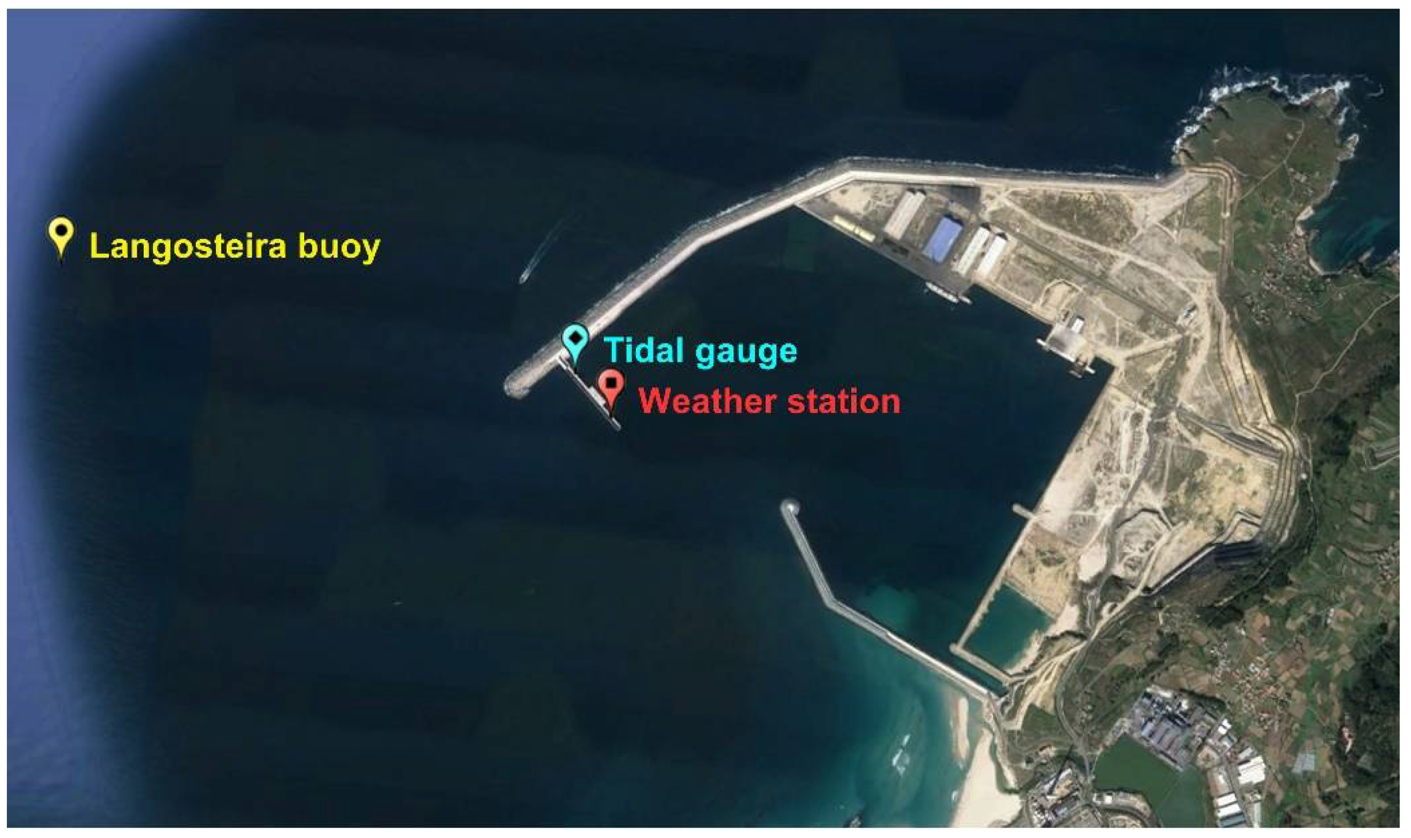
2.1. Dataset

The dataset described in [33], publicly available in [59], has been used to develop the prediction model presented in this work.

Data based on instrumental measurements of moored ship motions (6 DoF), obtained during several field campaigns undertaken in the Outer Port of Punta Langosteira (A Coruña, Spain) from 2015 to 2020, were collected in this dataset. The response of 46 different moored ships (25 general cargo ships and 21 bulk carrier ships) was measured by using three different synchronized devices, each for different motions/DoF. Pitch and roll motions were obtained from Inertial Measuring Unit (IMU) measurements. Sway and yaw motions were obtained from records of two laser distance meters that had been installed (one to the bow and the other to the stern of ships). Finally, surge and heave displacements were obtained by employing Computer Vision techniques applied to records from two cameras. Hourly parameters, in terms of mean, significant, and maximum values of each movement, are provided in the dataset. The corresponding date, number of berthing area (considered as representing the characteristics of each different berth), and number, type, and dimensions (length, L; breadth, B; deadweight, DWT) of ships are included in each hourly subset of data.

In addition, several instrumental-based met-ocean variables describing the climatic conditions associated with each hourly date record are also included in the available dataset. The instrumental data used to define those met-ocean variables come from three different sources.

First, outer-port wave conditions were defined in terms of significant wave height, Hs; wave peak period, Tp; and mean wave direction, Dm. These parameters, for each hourly sea state, were obtained from a coastal directional (Watchmate) buoy (Langosteira buoy, [60]) located in the vicinity of the port (Lon, Lat: 8.56° W, 43.35° N; 60 m depth; Figure 1). Secondly, wind conditions were provided, in terms of hourly mean wind velocity, Vw, and mean wind direction, Dw, from a weather station (Meteodata R.M. Young sensor) located at the perpendicular structure from main protection breakwater (Lon, Lat: 8.529° W, 43.345° N; Figure 1). Finally, the in-port significant wave height, Hsi, and sea level, SL, values are contained in each hourly subset of data. These latter parameters were obtained from the measurements of a tide gauge (Miros radar sensor; Langosteira tide gauge, [61]) located at the perpendicular structure from the main protection breakwater (Lon, Lat: 8.53° W, 43.35° N; Figure 1).

Additionally, as a final analysis in this research, infragravity wave descriptive variables have been added to the input dataset to evaluate the influence of such phenomena on the prediction model’s performance. In order to maintain the instrumental nature of the dataset, information of high-frequency sea level oscillations (HFSLO) based on the available raw 2-Hz data from the Miros radar sensor (Langosteira tide gauge) has been used according to [62]. The zero-order moment wave height (Hm_0IW) and the mean period (Tm_02IW) parameters, post-processed from the free surface spectra between frequencies of 1/600 Hz and 1/30 Hz, have been included in each hourly subset of data.

The available dataset is divided into two parts according to the separation into training and testing data for prediction models presented in [33]. Subsets of data corresponding to two specific ships (a small general cargo ship and a large bulk carrier) in the data sample were selected for testing and consequently extracted from the training database. The same division is applied in this work for development, and separately, for the validation of the proposed prediction model. In this way, the sizes of available databases for each type of motion are presented in

Table 1. Size of data samples used for training and testing the prediction model. Number of hourly subsets for each type of motion in the available dataset. Percentage (%) of data, with respect to the whole dataset, used for training and testing.

Type of Motion	Training Data	Testing Data
Surge	364 (95.8%)	16 (4.2%)
Sway	1451 (90.2%)	158 (9.8%)
Heave	364 (95.3%)	18 (4.7%)
Roll	1348 (96.4%)	51 (3.6%)
Pitch	1348 (96.4%)	51 (3.6%)
Yaw	1248 (88.8%)	158 (11.2%)

. It should be noted the lower number of data for surge and heave motions was due to occlusion events of the field of view of cameras during the field monitoring campaigns.

At this point, it should also be noted that gaps exist in the infragravity wave dataset, which provided discontinuous series of data throughout the duration of the monitoring campaigns. As explained in [62], availability and quality of these infragravity wave data are affected by sensor malfunctions, accidents, or external elements that can cause interferences in the radar beam. Due to error propagation, even small errors on the 2-Hz raw data from the sensor can produce meaningful gaps in the infragravity wave dataset.

Therefore, only the coincident time periods with available data from both the monitoring campaigns of moored ships and infragravity wave sensors have been used to evaluate the prediction model, including infragravity wave information (Hm_0IW and Tm_02IW). The reduced size of these data samples used for training and testing phases is shown in

Table 2. Size of data samples used for training and testing the prediction model including infragravity wave information in the input dataset. Number of the available hourly subsets for each type of motion. Percentage (%) of data, with respect to the whole dataset, used for training and testing.

Type of Motion	Training Data	Testing Data
Surge	131 (90.3%)	14 (9.7%)
Sway	708 (85.7%)	118 (14.3%)
Heave	131 (89.1%)	16 (10.9%)
Roll	787 (94.4%)	47 (5.6%)
Pitch	787 (94.4%)	47 (5.6%)
Yaw	683 (85.3%)	118 (14.7%)

.

2.2. Machine Learning Inference Methodologies for Prediction of Moored Ships’ Motions

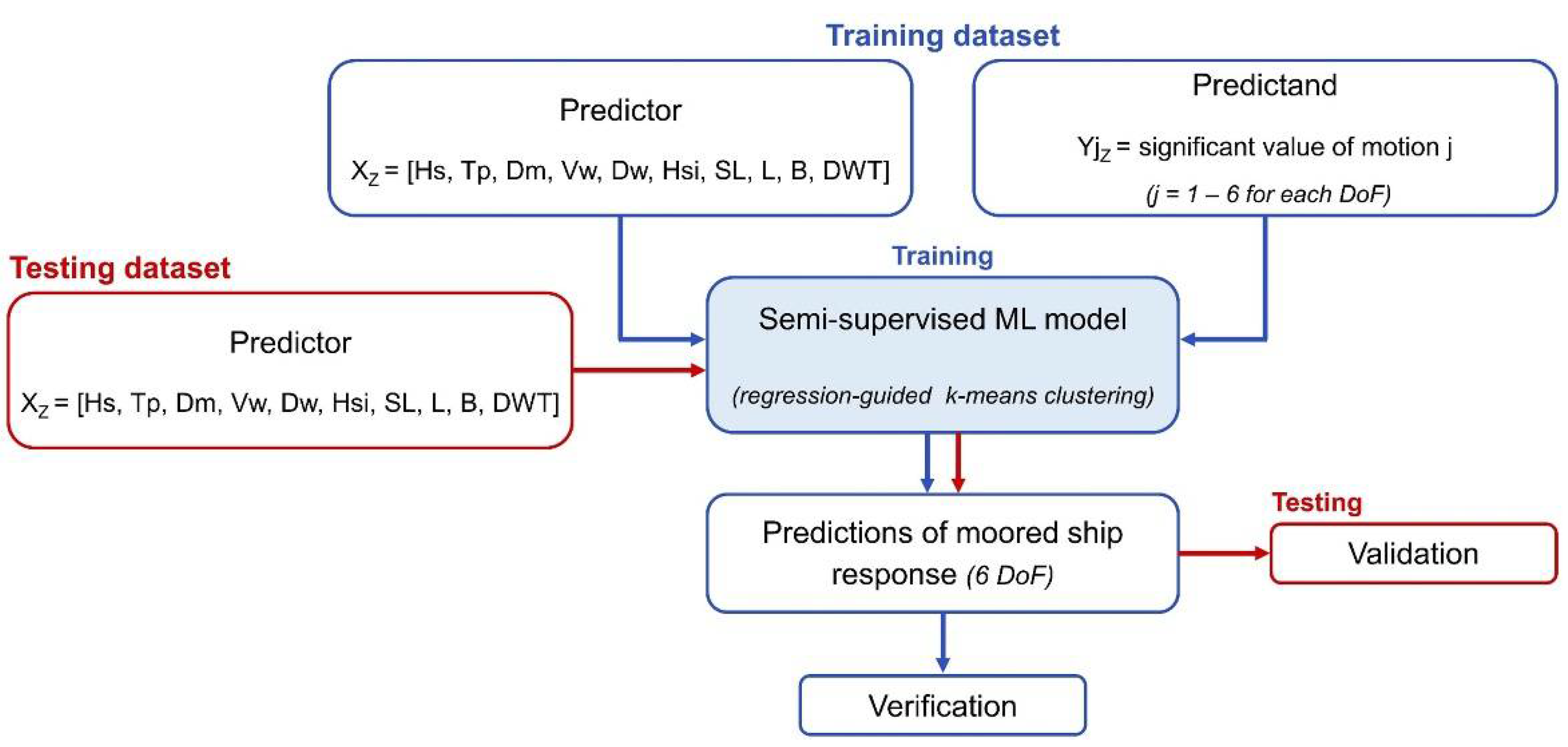
2.2.1. Semi-Supervised Learning-Based Model

In this section, the general description of the methodology, based on semi-supervised ML techniques, for the prediction of moored ship response is presented. The general framework of the methodology is shown in Figure 2, where the flowcharts for the training and testing phases are presented.

Specifically, the proposed methodology is based on the regression-guided k-means clustering method [54]. The complete procedure can be divided into the following 6 steps:

• Definition of predictor (X) and predictand (Y) matrices.
• Standardization of X and Y variables in order to equalize the contribution of the different variables.
• Multiple linear regression fitting, establishing the linear dependency function between the response variables (predictand, Y) and the input variables (predictor, X). The linear relationship is defined by the expression:

  Y = X·B + E

  (1)

  where X and Y are the predictor and predictand matrices, respectively; B is the matrix of fitting coefficients from the multiple linear regression; and E is the matrix of residual error between estimations—obtained from regression—and real measured values. The estimations from the regression are obtained as Ŷ = X·B.
• Weighted concatenation of the X matrix and the Ŷ predictions through the following expression:

  Z = [(1 − α)·X, α·Ŷ]

  (2)

  where α is the weighting factor.
  When α = 0, only the X predictor matrix is considered in the clustering procedure, resulting in a completely unsupervised learning-based method. Conversely, when α = 1, only the Ŷ predictions matrix is considered in the classification procedure, resulting in a completely supervised learning-based method. When 0 < α < 1, an intermediate semi-supervised learning-based model is defined.
• K-means algorithm-based clustering of Z. By means of an iterative procedure, each subset of data is grouped to the nearest cluster centroid in terms of Euclidean distance. The positions of the cluster centroids V are calculated as the mean value of all the subsets of data contained in each cluster “k”. Thus, the positions of cluster centroids are updated at each iterative step.

  $$\mathrm{Vk}={\displaystyle \sum }_{\mathrm{i}=1}^{\mathrm{Nk}}\frac{\mathrm{Zi}}{\mathrm{Nk}}$$

  (3)

  where Nk is the number of elements in the k-th cluster.
  Instead of random initialization, the initial position of cluster centroids is established by a previous application of the Max-Diss algorithm to the Z dataset. In this way, an initial set of centroids distributed throughout the n-dimensional space of the Z matrix is defined to start the iterative clustering procedure.
  Once the clustering is completed, the prediction model is defined by the mean (μ) and standard deviation (σ) of predictand values in each cluster.
• Prediction of output variables. The predictions of response variables are assigned as the value of the nearest centroid (i.e., k-nearest algorithm) through a Euclidean distance evaluation.

Finally, two other prediction models (a supervised and an unsupervised one) have been developed in order to analyze and compare the performance of different existing ML techniques for the prediction of the motions of moored ships.

2.2.2. Supervised Learning-Based Model

An inference model based on the multiple linear regression algorithm is created by following the previously described steps from 1 to 3. The estimations Ŷ from the regression model are directly considered predictions.

2.2.3. Unsupervised Learning-Based Model

The proposed methodology’s unsupervised version has also been considered to generate another prediction model. In this case, steps 3 and 4 (relative to the regression guide) do not apply. The k-means clustering algorithm (step 5) is directly applied to standardized predictor matrix X. In this way, the influence of predictand variables is not considered in the clustering procedure nor, therefore, in learning the prediction model.

2.3. Application and Performance Assessment

The inference models based on the previously described ML methodologies are first created and evaluated by using the available dataset [33,59]. Secondly, an extended version of the semi-supervised learning-based model, with infragravity wave parameters introduced as predictor variables, is presented.

2.3.1. Initial Version of the Model

As explained in Section 2.1, each hourly subset of data comprises several concomitant data values, which can be divided into predictor (input data) and predictand (output data) variables in the prediction model. That is, parameter values of moored ship motions are used for predictand definition, while met-ocean variables, as well as those related to ship characteristics, are used for predictor definition. According to [33], only the significant value of ship motions is considered as the predictand in the prediction model presented in this work. Series of mean and maximum values are not used. The predictor matrix is defined by the following variables: outer-port Hs, Tp, and Dm; Vw and Dw of wind; in-port Hsi and SL; and L, B, and DWT of ship. The identifying number of berthing areas is not defined as a predictor variable in this work, but each different berthing area is separately analyzed in the proposed prediction model. In summary, for each berthing zone (z), the predictor (X) and predictand (Y) matrices are structured as follows:

X_Z = [Hs, Tp, Dm, Vw, Dw, Hsi, SL, L, B, DWT]

Yj_Z = significant value of motion j (with j = 1 to 6 for each type of motion)

The available dataset is divided into two parts according to the separation into training and testing data for prediction models presented in [33], as explained in Section 2.1. The sizes of the different data samples used for each type of motion are presented in Table 1.

Based on the previously described methodology, the inference models proposed from the predictor and predictand matrices are created.

In the regression-guided clustering methodology, the value of two factors must be defined, affecting the quality of the obtained results. On the one hand, the number of clusters in the clustering procedure (step 5 of the methodology), and on the other hand, the α factor to be considered in the weighted concatenation of matrices X and Ŷ (step 4 of the methodology). In order to evaluate the influence of these values on the final predictions from the model, a sensibility analysis has been performed. Different squared cluster sizes (4, 25, 36, 49, 64, 81, 100, 121, and 144 clusters) and different values of α (from 0 to 1, with increments of 0.1) for each number of clusters have been considered and separately evaluated for each type of motion. A total of 90 configurations (9 cluster sizes x 10 values of α) have been analyzed for each of the 6 DoF. The quality of the predicted results obtained, both in the training and validation phases, for each of the 90 configurations, has been evaluated using two indices: the Root Mean Square Error (RMSE) and correlation ratio (R²) between predictions and measured data. The obtained results are presented in Section 3.1.1. The optimal values for the number of clusters and α factor have been identified from the analysis of these two evaluating indices. These optimal values have been selected as those achieving the most accurate predictions in the testing phase, although they do not show the best goodness of fit in the training phase. Moreover, practical criteria delimiting the corresponding ranges of those factors for each type of motion have been defined from the analysis. It should be noted that these values are applicable as long as data samples with similar characteristics (e.g., size, dispersion, etc.) are used to create the model. In order to determine the validity range of these practical criteria, the coefficient of variation (CV) of predictand and the proportion of variance explained (EV) of predictor clustering have also been indicated in Section 3.1.1. According to [54], CV and EV are given by:

CV = σ/μ

(4)

EV = 1 − SSE/SSE_T

(5)

where SSE is the sum of the squared errors in the different clusters, and SSE_T is the total squared error of the dataset.

2.3.2. Extended Version with IW Predictor Variables

This section presents an extended version of the semi-supervised learning-based model. An extension of the predictor matrix, including the infragravity wave descriptive parameters, has been created. Therefore, the extended predictor matrix is defined by:

X_Z = [Hs, Tp, Dm, Vw, Dw, Hsi, SL, L, B, DWT, Hm_0IW, Tm_02IW]

As explained in Section 2.1, data gaps exist in time series of the infragravity wave parameters obtained from the sensor. Therefore, the coincident time periods with available data from both the monitoring campaigns of moored ships and infragravity wave sensors have been used to evaluate the prediction model including infragravity wave information. The reduced size of these data samples used for training and testing phases are shown in Table 2. As can be seen, the size of the training dataset is considerably reduced, while the proportion of available testing data remains similar (slightly lower).

The sensitivity analysis for the number of clusters and α factor has been carried out analogously to the previous one for the new input dataset. The obtained results are presented in Section 3.2.1.

3. Results and Discussion

In this section, the performance of the three prediction models based on the different proposed methodologies applied to the available dataset [33,59] is evaluated and compared with other existing techniques.

Additionally, a final evaluating analysis between both versions of the semi-supervised learning-based models is presented. The results obtained from the extended version with the IW predictor variables are compared with those based on the traditional wave, wind, and sea level predictor variables.

3.1. Initial Version of the Model

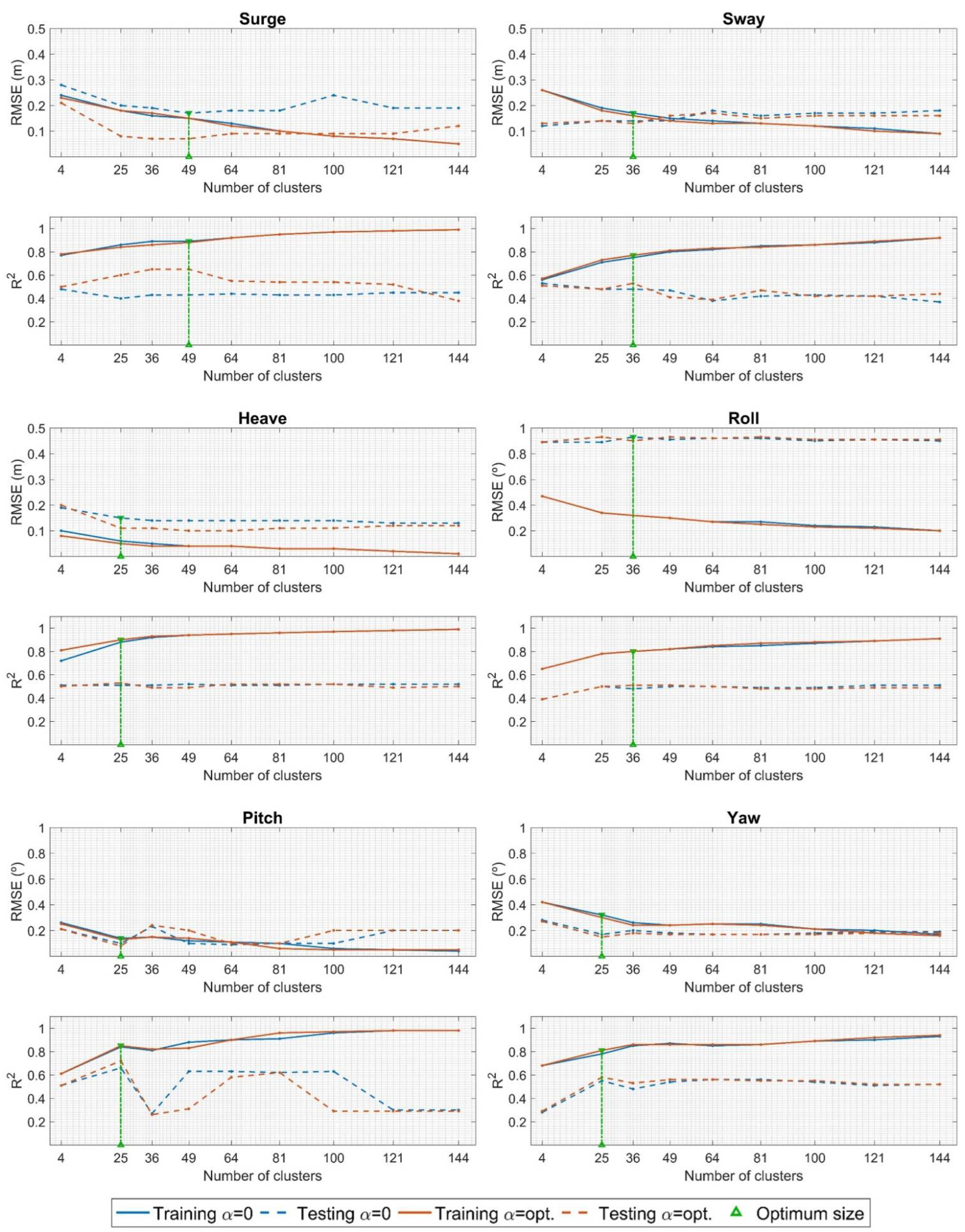
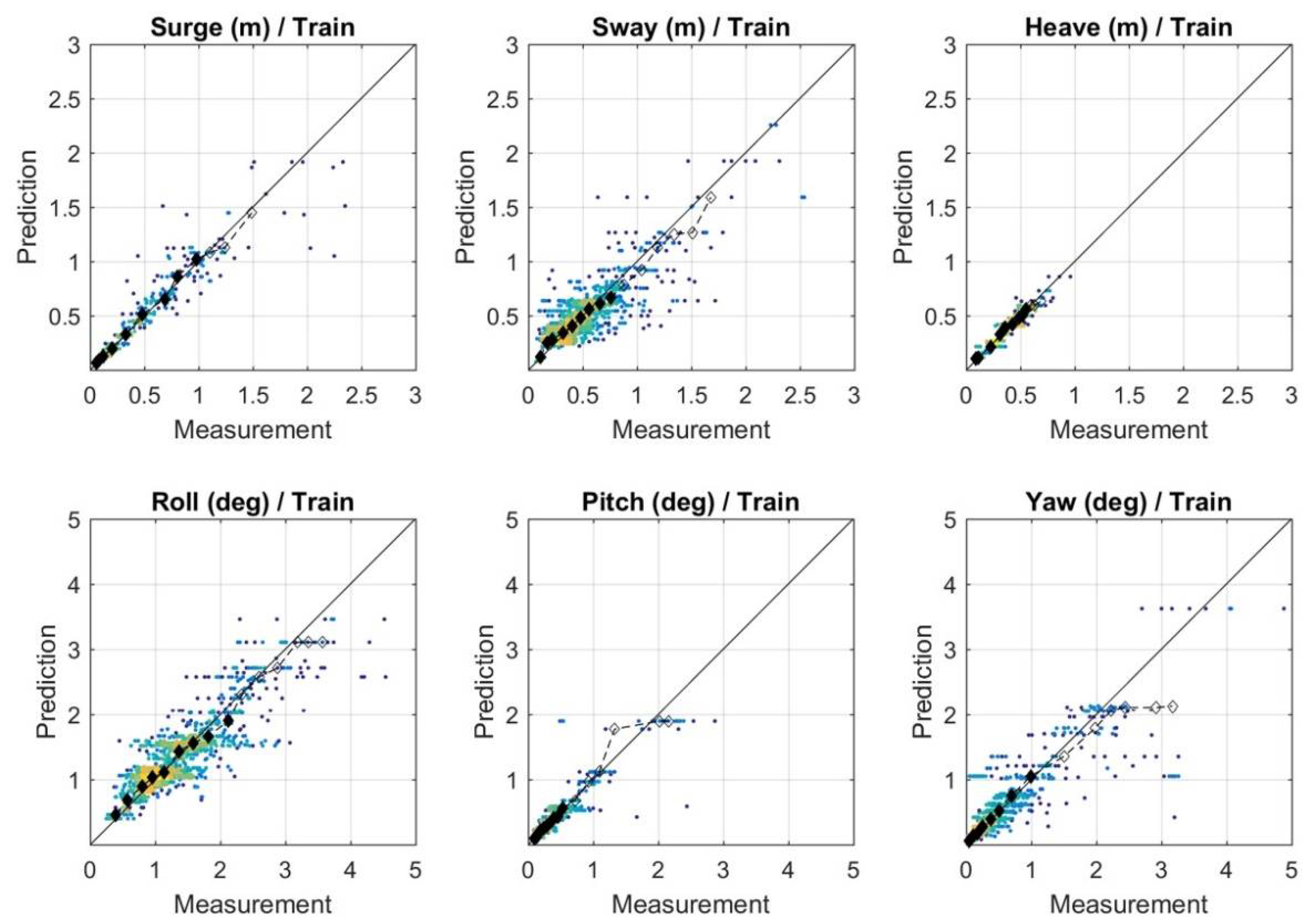
3.1.1. Performance Assessment

As explained in Section 2.3.1, a sensitivity analysis of the influence of two factors (number of clusters and α weighting factor) on the quality of predictions from both models based on the semi- and unsupervised k-means clustering algorithm has been carried out. The results obtained, both in the training and validation phases, for each model configuration have been evaluated in terms of RMSE and R² coefficients. The optimal values of those factors, for each type of motion, have been identified as those achieving the most accurate predictions in the testing phase. The results are presented in

Table 3. Practical criteria to define the values for “number of clusters” and “α” in the application of the methodology. Validity ranges are determined by CV and EV.

Type of Motion	Number of Clusters		α Factor		CV		EV
	Optimum	Range	Optimum	Range	Optimum	Range	Optimum	Range
Surge	49	49	0.6	[0.6, 0.7]	0.20	[0.20, 0.21]	0.97	0.97
Sway	36	[25, 36]	0.3	[0.2, 0.3]	0.31	[0.31, 0.33]	0.84	[0.80, 0.84]
Heave	25	25	0.6	[0.5, 0.7]	0.11	[0.11, 0.12]	0.91	[0.91, 0.92]
Roll	36	[25, 36]	0.1	[0.1, 0.4]	0.24	[0.24, 0.25]	0.86	[0.82, 0.86]
Pitch	25	25	0.2	[0.1, 0.4]	0.22	[0.22, 0.23]	0.82	0.82
Yaw	25	[25, 36]	0.3	[0.2, 0.4]	0.47	[0.36, 0.49]	0.82	[0.82, 0.86]

. The corresponding CV and EV coefficients are also indicated in Table 3.

The results obtained for each type of motion, both for the optimal values of α and for α = 0 (unsupervised k-means algorithm), for each of the clustering sizes analyzed are presented in Figure 3. The evaluating indices RMSE and R² are represented, both for the verification phase after the training/learning of the model and for the validation phase of the predictions obtained with the previously trained model for the testing data sample.

As can be seen for all the six DoF, higher-quality predictions were obtained from the model based on the regression-guided clustering method (α ≠ 0) compared to that based on the unsupervised k-means algorithm (α = 0). Similar evaluating indices can be observed in the verification results of the training phase for both the semi- and unsupervised learning-based models. Nevertheless, the improvement achieved for the optimal α values compared to α = 0 can be more clearly appreciated in the validation of the testing phase.

In general, for the training verification phase in all the figures, the progressive improvement of the evaluating indices (i.e., the decreasing RMSE and increasing R²) as the number of clusters increases in both the guided and not-guided clustering procedures can be observed. This behavior was expected since the data subsets were located closer to their values for the larger number of clusters. The extreme definition would be reached for a number of clusters equal to the sample size, where each centroid would fit with its unique data subset. However, for the testing phase, these trends change from a certain size/number of clusters. For example, for the surge motion results in Figure 3, an RMSE reduction was observed between 4 and 25 clusters. From 25 clusters, the RMSE is practically stabilized until the size of 49 clusters, from which the predictions start worsening. Similarly, the increasing trend of the R² between 4 and 36 clusters can be observed, stabilizing and then worsening from the size of 49 clusters. An overfitting of the prediction model from such a number of clusters in the training phase is verified, with a better goodness of fit in the verification/training phase, but it is worsening in the validation/testing phase. Similar behaviors can be observed for the other movements, allowing for the identification of the optimum number of clusters to be established in the clustering procedure for each type of motion. In this way, the optimal values have been identified as those achieving the best evaluating indices in the validation/testing, despite not corresponding with the best goodness of fit in training.

The scatter plots of the comparison between the semi-supervised ML-based model predictions and the measured data from field campaigns are represented in Figure 4 and Figure 5 for the training and testing phases, respectively. The goodness of fit obtained for the training and testing phases for each type of motion can be observed. In general, an adequate correlation between the predictions and measurements was obtained for all the DoF training and testing phases, except for the roll motion in the testing phase where a considerable deviation is shown. As discussed below, this deviated roll behavior is generally observed for all the techniques considered for the analysis and comparison in this work (see

Table 4. Comparison of different ML and DL algorithms for prediction of the 6 DoF of moored ship motions. Quantification of error, RMSE; correlation, R². In green, the highest values of fit, and in red, the poorest value of fit, for each case of all algorithms. The values of the measurements range for each type of motion are also indicated. Training phase.

Training
		Surge		Sway		Heave		Roll		Pitch		Yaw
		R2	RMSE (m)	R2	RMSE (m)	R2	RMSE (m)	R2	RMSE (°)	R2	RMSE (°)	R2	RMSE (°)
Supervised ML	Multiple linear regression 1	0.82	0.20	0.72	0.19	0.90	0.05	0.73	0.39	0.70	0.21	0.79	0.31
	Gradient Boosting 2	0.86	0.11	0.92	0.04	0.92	0.03	0.91	0.11	0.98	0.04	0.95	0.06
Unsupervised ML	K-means 1	0.89	0.15	0.75	0.17	0.94	0.04	0.78	0.34	0.84	0.14	0.78	0.32
Semi-supervised ML	Regression-Guided K-means 1	0.88	0.15	0.77	0.16	0.90	0.05	0.80	0.32	0.85	0.13	0.81	0.30
Deep Learning	Artificial Neural Networks 2	0.99	0.03	0.99	0.02	0.95	0.05	0.99	0.06	0.98	0.02	0.98	0.01
	Range	2.3 m		2.5 m		0.9 m		4.3°		2.8°		4.8°

¹ Developed in this work. ² Developed in [33].

and

Table 5. Comparison of different ML and DL algorithms for prediction of the 6 DoF of moored ship motions. Quantification of error, RMSE; correlation, R². In green, the highest values of fit, and in red, the poorest value of fit, for each case of all algorithms. Testing phase.

Testing
		Surge		Sway		Heave		Roll		Pitch		Yaw
		R2	RMSE (m)	R2	RMSE (m)	R2	RMSE (m)	R2	RMSE (°)	R2	RMSE (°)	R2	RMSE (°)
Supervised ML	Multiple linear regression 1	0.51	0.23	0.50	0.15	0.55	0.08	0.47	1.06	0.35	0.19	0.17	0.37
	Gradient Boosting 2	-	0.39	-	0.11	-	0.09	-	1.04	-	0.24	-	0.28
Unsupervised ML	K-means 1	0.43	0.17	0.48	0.14	0.52	0.14	0.50	0.89	0.66	0.10	0.55	0.17
Semi-supervised ML	Regression-Guided K-means 1	0.65	0.07	0.53	0.13	0.53	0.11	0.51	0.90	0.72	0.08	0.58	0.15
Deep Learning	Artificial Neural Networks 2	-	0.10	-	0.15	-	0.12	-	0.90	-	0.11	-	0.15

¹ Developed in this work. ² Developed in [33].

).

From the analysis of the results of the training phase, the most correlated results (Figure 4 and Table 4) were observed for the two types of movements with the smallest datasets (surge and heave). This would be expected due to the lower amount of data to be clustered, which results in a tighter value grouping within each cluster. This is also consistent with the highest EV coefficients shown for these two movements in Table 3. For the heave motion, a good fit is obtained over the whole range of measurements (Figure 4), although it is narrower (0.9 m; Table 4) than the other movements. This would also be expected since this motion type is the most directly influenced by waves and not by other aspects that are more difficult to capture, such as the effects of mooring lines. From the analysis of the surge scatter plot in Figure 4, larger deviations (underestimation) of the predictions compared to the measurements can be observed for the largest instrumental values (from surge measurements of 2 m). This reveals the greater complexity of the characterization of this DoF from the predictor variables considered. Indeed, despite the reduced number of available data, the surge motion presents the highest optimum number of clusters (Table 3). In contrast to heave, the surge motion is highly influenced by the effects of mooring lines (non-linear behavior, pretension, mooring plan, etc.), which may not be fully represented in the model (partly due to the predictor variables and their nature, and partly due to the inference relationships established). Similarly, the deviations (higher dispersion in Figure 4 and poorer correlation coefficients in Table 4) between the predicted and measured values for sway and yaw motions could be because of the influence of the mooring system on these horizontal motions. As it can be observed in Figure 4 and Table 4, the pitch motion is the rotational DoF with the highest correlation between the predictions and measured data. The pitch measurements are also contained within the narrowest range compared to roll and yaw (2.8⁰; Table 4). Similar to that mentioned for heave, pitch is a vertical movement greatly influenced by waves rather than by the mooring configuration, so apparently, the inference relationships between predictand and predictor variables are better identified for these DoF in the model. Finally, a dispersion is also observed in the scatter plot for roll motion in the training phase. The possible causes are discussed in more detail below for the analysis of the results from the testing phase.

From the analysis of the results from the testing phase (Figure 5 and Table 5), an adequate goodness of fit of the predictions is shown for all the movements except for the roll motion where a notable deviation was observed. Different causes may underlie these roll deviations. It could be the DoF with the greatest associated uncertainty introduced from different sources. First, those differences between the measurements and predictions could be due to higher variations in the characterization of this motion type for the two separated ships (berthing/mooring scenarios) used in the testing phase. As mentioned in [33], a greater variability of the roll motion measurements is shown for similar met-ocean predictor variables, which makes it more difficult for the model to establish the inference relationships. A second possible reason could be a higher difficulty involved in measuring and reproducing this movement since the roll motion is restricted to one side by the berthing structure. Another possible reason could be the varying aspects influencing the roll motion more intensely than the other DoF during the operations/berthing time, such as inertial changes existing during the loading/unloading activities, changes in the mooring line tensions due to variations in the sea level or the ship’s draft (loaded/ballast conditions), or the relative position and orientation of the ship with respect to the multidirectional in-port wave patterns occurring at different berthing areas. Many of these mentioned aspects are not (or are only limitedly) represented by aggregated parameters used for the model-learning and prediction. Finally, the possible limitations mentioned in [33] concerning the measured data (small dataset size, bias, and noise) should be pointed out.

Further analysis of the possible causes of these roll deviations will be contemplated in future works where the authors will expect to have detailed information concerning the met-ocean climate, field campaign development, and field data acquisition (e.g., boundary conditions; disaggregated definition of met-ocean forcings; sensitivity, resolution, and sampling frequency of the monitoring equipment; sensor calibration; etc.).

3.1.2. Comparative Analysis of Different AI Techniques for Prediction of Moored Ships’ Motions

Finally, a comparative analysis of the performance of different AI techniques (multiple linear regression, gradient boosting, unsupervised k-means clustering, regression-guided k-means clustering, and artificial neural networks algorithms) applied to the prediction of the movements of moored ships has been performed. The evaluation of the predictive performance of each different technique-based model, in terms of RMSE and R², is summarized in Table 4 for the verification of the training phase, and in Table 5 for the validation of the testing phase. In these tables, the poorest and the highest goodness of fit values are indicated in red and green, respectively.

It should be noted that the prediction models based on the gradient boosting algorithms and artificial neural networks from [33] as well as the three prediction models developed in this work—based on the semi-supervised regression-guided k-means, unsupervised k-means, and multiple linear regression algorithms—have been created from the same available dataset in both the training and testing phases.

As it can be seen from this comparison, the most correlated results of the training phase were obtained from the ANN-based model, with RMSE and R² values close to 0 and 1, respectively. On the other hand, in the training phase, the poorest goodness of fit values were obtained for the results from the model based on the multiple linear regression algorithm (R² between 0.70 and 0.90, for different movements, and RMSE/measurements range ratios between 5.6% and 9.1%; Table 4). However, in the testing phase, the best results, for most of the movements, were obtained from the proposed model based on the regression-guided k-means algorithm (R² between 0.51 and 0.72, for different movements, and RMSE/measurements range ratios between 2.9% and 20.9%; Table 5).

From the analysis of the results obtained in each phase (training/verification and testing/validation), an apparent overfitting of the ANN-based model may be appreciated, due to the relative reduction in the predictions quality in the testing phase compared to the verification of the training (where the highest goodness of fit was noted).

Finally, as previously commented, the poorest predicted results were obtained for the roll motion, from all the different prediction models analyzed. As explained above, roll motions could be considered the DoF with the greatest associated uncertainty introduced from different sources. Further analysis of roll deviations is intended to be carried out in future works.

As a summary from the analysis of the comparison of different ML- and DL-based prediction models to infer the response of the moored ships in six DoF, good correlation results (R² ≥ 0.70; Table 4) were obtained in general for all the models considered in the analysis. In the testing phase (Table 5), poorer evaluating indices were obtained. However, from this comparative analysis, the proposed prediction model based on the regression-guided k-means clustering algorithm has been identified as the best performing of the five different models analyzed for predicting the movements of moored vessels. Therefore, the capabilities of the proposed model for predicting the response of berthed ships and consequently the port operability/downtime for port management has been demonstrated.

3.2. Extended Version with IW Predictor Variables

In this section, the previously validated semi-supervised ML methodology proposed for the prediction of moored ships’ movements is applied with an extended predictor matrix X including the infragravity wave descriptive parameters Hm_0IW and Tm_02IW.

3.2.1. Performance Assessment

Since a new dataset with different characteristics was used, a new sensibility analysis for the clustering size and α factor was performed. The obtained results are presented in

Table 6. Obtained results from the sensitivity analysis for “number of clusters” and “α” in the extended version with IW predictor variables. Corresponding CV and EV coefficients.

Type of Motion	Number of Clusters	α Factor	CV	EV
	Optimum	Optimum	Optimum	Optimum
Surge	25	0.4	0.15	0.99
Sway	25	0.3	0.38	0.80
Heave	25	0.5	0.05	0.99
Roll	25	0.2	0.24	0.81
Pitch	49	0.4	0.16	0.89
Yaw	36	0.3	0.37	0.86

. The differences with those presented in Table 3 may be due, on the one hand, to the addition of the new IW predictor variables, and on the other hand, to the different characteristics (mainly in size) between the datasets. At this point, the lower representativeness of these values with respect to those presented in Table 3, due to the reduced size of the data samples used here, should be noted.

3.2.2. Comparative Analysis with the Initial Version of the Model for Prediction of Moored Ships’ Motions

Due to the previously explained reduction in size of the training and testing data samples when introducing IW parameters (Section 2.1), and in order to obtain comparable results, the clustering procedure has been repeated with the reduced initial predictor matrix (without IW). The obtained results, in both the training and testing phases, are presented in

Table 7. Evaluation of the influence of infragravity wave parameters introduced as predictor variables in the model. Quantification of error, RMSE, and correlation, R², of predictions of the 6 DoF of moored ship motions. Comparison between semi-supervised ML-based models with and without IW; in green, improvement, and in red, worsening.

Training
		Surge		Sway		Heave		Roll		Pitch		Yaw
		R2	RMSE (m)	R2	RMSE (m)	R2	RMSE (m)	R2	RMSE (⁰)	R2	RMSE (⁰)	R2	RMSE (⁰)
Semi-supervised ML	Regression-Guided K-means; initial	0.88	0.15	0.77	0.16	0.90	0.05	0.80	0.32	0.85	0.13	0.81	0.30
	Regression-Guided K-means; without IW	0.95	0.10	0.75	0.15	0.95	0.03	0.83	0.30	0.90	0.11	0.81	0.30
	Regression-Guided K-means; with IW	0.95	0.11	0.72	0.17	0.94	0.03	0.82	0.31	0.93	0.09	0.82	0.29
Testing
		Surge		Sway		Heave		Roll		Pitch		Yaw
		R2	RMSE (m)	R2	RMSE (m)	R2	RMSE (m)	R2	RMSE (m)	R2	RMSE (m)	R2	RMSE (m)
Semi-supervised ML	Regression-Guided K-means; initial	0.65	0.07	0.53	0.13	0.53	0.11	0.51	0.90	0.72	0.08	0.58	0.15
	Regression-Guided K-means; without IW	0.51	0.14	0.46	0.13	0.52	0.11	0.53	0.91	0.65	0.09	0.55	0.13
	Regression-Guided K-means; with IW	0.49	0.14	0.49	0.12	0.51	0.10	0.53	0.85	0.69	0.08	0.52	0.13

. The values in grey text correspond to the previously presented results obtained from the semi-supervised ML-based model. The analogous results obtained by using the reduced datasets with and without IW variables are shown in black text. The variations in the results due to the addition of infragravity wave descriptive variables in the predictor matrix are represented in green (improvement) and red (worsening) fill colors.

From the analysis, the variation of the results obtained in this section for the model without IW, compared to the previous one, can be observed due to the dataset size reduction. Through a comparison between the evaluating indices of the models with and without IW, slightly improved predictions can be seen for the model with IW, mainly in the validation phase for most of the six DoF. Different factors, such as harbor configuration (geometry, port contours, typology of structures, etc.) as well as those relative to the ship and the berthing/mooring system (size, loading condition, mooring plan, pretension, etc.), have an impact on the influence of the infragravity waves on the response of the moored ship. However, the effects of infragravity waves would be expected, on the one hand, on the heave, roll, and pitch, depending on the ship dimensions with respect to the wavelength, and on the other hand, on the surge, sway, and yaw motions, depending on the relation of the infragravity wave period to the natural/resonant period of mooring system. The obtained results seem to be consistent with these aspects, thus demonstrating the capability of the prediction model.

4. Conclusions

In this paper, a semi-supervised Machine Learning-based model for the prediction of moored ships’ motions is proposed.

A statistical prediction model based on a regression-guided k-means clustering algorithm has been developed. An unsupervised k-means clustering-based model and a supervised learning-based prediction model based on a multiple linear regression have also been created for comparison. A sensitivity analysis has been carried out, evaluating the influence of the two factors to be defined in the methodology (number of clusters and α weighting factor) on the quality of predictions from both models based on the semi- and unsupervised k-means clustering algorithm. The optimal values of those factors, for each type of motion, have been identified. A performance assessment of the different models has been performed. From the comparison of the results obtained from the three proposed models, the highest performance was observed for the semi-supervised ML-based model, while the lowest goodness of fit predictions were obtained for the multiple linear regression-based model.

In addition, a comparative analysis with other existing models, based on different supervised (gradient-boosting algorithm) and deep learning (ANN) techniques, has been performed. In the testing phase, more accurate predictions were obtained with the proposed semi-supervised learning-based model compared to the other inference techniques.

In general, an adequate goodness of fit of the predictions is shown for all the movements in both the training and testing phases, except for the testing roll motion where a notable deviation was observed. As explained, this deviated roll behavior was generally observed for all the models analyzed and compared in this work (see Table 4 and Table 5). A further analysis will be contemplated in future works, wherein the authors expect to have detailed information concerning the met-ocean climate, field campaign development, and field data acquisition. It is expected that more detailed information on the possible sources of error and the uncertainty introduced will lead to stronger conclusions about the causes of these roll prediction deviations.

Finally, a comparison to evaluate the influence of infragravity wave parameters introduced as predictor variables in the prediction model has been performed. Slightly improved predictions have been observed from the model including infragravity wave parameters, mainly in the validation phase for most of the six degrees of freedom.

To conclude, the highest performance of the proposed semi-supervised Machine Learning-based model for predicting the movements of moored ships has been demonstrated from a comparative analysis of different AI techniques (multiple linear regression, gradient boosting, unsupervised k-means clustering, regression-guided k-means clustering, and artificial neural networks algorithms). The analysis has revealed the capabilities of the proposed model for use as an assistance tool for the management of berths and port operations in harbors. In addition, the simplicity and robustness of the implementation and maintenance of a prediction model based on the proposed methodology should be pointed out, compared to the complexity demanded by other types of techniques, such as Artificial Neural Networks, to define and adjust the structure and required parameters. This could be a relevant aspect in large harbors consisting of many different port terminals and berthing areas. In addition, it should be noted that not only predictions but also the associated uncertainty can be inferred from the standard deviation of the predictions. Both the intrinsic variability of the base dataset as well as that due to the inference method adopted are encompassed by such an uncertainty value

Furthermore, the proposed inference model can also be directly applied as a moored ship forecast system to predict the movements of berthed ships in six DoF by defining the predictor matrix through available information from met-ocean forecast services and port activities planning.

Note that the predictive model described has been defined, in general terms, to be applied to any port with the objective of predicting the movements of moored vessels. However, it should be noted that the model adjustment has been performed for a specific location, the Outer Port of Punta Langosteira, to show its predictive capability. In this case, the data corresponding to the vessels that moored at the port during the the field campaign have been used, in addition to the configuration of the mooring modes and the climatic information. Nevertheless, the application of the predictive model to another port with a different fleet of ships, maritime climate, port geometry, and mooring modes, must always be performed after an adequate adjustment of the model to the specific field data by characterizing the moored-ship behavior of each berthing area and its interaction with the port’s geometry and the environment.

References

1. Puertos del Estado; Ministerio de Fomento. Recommendations for Maritime Works—Series 3—Planning, Management and Operation in Port Areas: ROM 3.1-99—Design of the Maritime Configuration of Ports, Approach Channels and Harbour Basins; Puertos del Estado: Madrid, Spain, 1999.
2. Puertos del Estado; Ministerio de Fomento. Recommendations for Maritime Works—Series 2—Inner Harbor Structures: ROM 2.0-11—Recommendations for the Design and Construction of Berthing and Mooring Structures; Puertos del Estado: Madrid, Spain, 2012.
3. Working Group PTC II-24. Criteria for Movements of Moored Ships in Harbours: A Practical Guide; Supplement to Bulletin No 88; PIANC General Secretariat: Brussels, Belgium, 1995; Volume 88. [Google Scholar]
4. MarCom Working Group. Criteria for the (Un)loading of Container Vessels; PIANC Report 115; PIANC General Secretariat: Brussels, Belgium, 2012. [Google Scholar]
5. Bruun, P. Breakwaters versus Mooring. Dock Harb. Auth. 1981, XLII, 730. [Google Scholar]
6. Thoresen, C.A. Port Designer’s Handbook: Recommendations and Guidelines; Thomas Telford Publishing: London, UK, 2003. [Google Scholar]
7. D’Hondt, E. Port and terminal construction design rules and practical experience. In Proceedings of the 12th International Harbour Congress, Antwerp, Belgium, 22–27 September 1999. [Google Scholar]
8. Ueda, S.; Shiraishi, S. The Allowable Ship Motions for Cargo Handling at Wharves; Port and Harbour Research Institute—PHRI: Yokosuka City, Japan, 1988; Volume 27, pp. 3–61.
9. Gaythwaite, J.W. Mooring of Ships to Piers and Wharves; ASCE Manuals and Reports on Engineering Practice; American Society of Civil Engineers: Reston, VA, USA, 2014. [Google Scholar] [CrossRef]
10. Danish Hydraulic Institute (DHI). MIKE 21 Maritime—MIKE 21 Mooring Analysis—User Guide 2022; Danish Hydraulic Institute (DHI): Hørsholm, Denmark, 2022. [Google Scholar]
11. Mynett, A.E.; Keuning, P.J.; Vis, F.C. The Dynamic Behaviour of Moored Vessels Inside a Habour Configuration; Delft Hydraulics Laboratory: Birmingham, UK, 1985. [Google Scholar]
12. Maritime Research Institute Netherlands (MARIN). aNyMOOR.TERMSIM; Maritime Research Institute Netherlands (MARIN): Wageningen, The Netherlands; Available online: https://www.marin.nl/en/facilities-and-tools/software/ (accessed on 12 July 2022).
13. Tension Technology International. OPTIMOOR. Mooring Analysis Software for Ships & Barges; Technical Notes 01; Tension Technology International: Schoonhoven, The Netherlands, April 2016. [Google Scholar]
14. Arcadis. SHIP-MOORINGS, Version 10; Arcadis: Amsterdam, The Netherlands, 2016. [Google Scholar]
15. Pinheiro, L.V.; Fortes, C.J.E.M.; Santos, J.A.; Fernandes, J.L.M. Numerical simulation of the behaviour of a moored ship inside an open coast harbour. In Proceedings of the 5th International Conference on Computational Methods in Marine Engineering, MARINE 2013, Hamburg, Germany, 29–31 May 2013. [Google Scholar]
16. Pinheiro, L.V.; Santos, J.A.; Fortes, C.J.; Fernandes, J.L. Numerical Software Package SWAMS—Simulation of Wave Action on Moored Ships; DuraSpace: Atlanta, GA, USA, 2013. [Google Scholar]
17. Pinheiro, L.V.; Fortes, C.; Santos, J.; Fernandes, J.L. Coupling of a Boussinesq Wave Model with a Moored Ship Behavior Model. Coast. Eng. Proc. 2012, 1, 69. [Google Scholar] [CrossRef]
18. Bhautoo, P.S. Dynamic mooring analysis to investigate long period wave-induced vessel motions at Esperance Port. In Proceedings of the Australasian Coasts and Ports 2017 Conference, Cairns, Australia, 21–23 June 2017. [Google Scholar]
19. Bingham, H.B. A hybrid Boussinesq-panel method for predicting the motion of a moored ship. Coast. Eng. 2000, 40, 21–38. [Google Scholar] [CrossRef]
20. Christensen, E.D.; Jensen, B.; Mortensen, S.B.; Hansen, H.F.; Kirkegaard, J. Numerical simulation of ship motion in offshore and harbour areas. In Proceedings of the International Conference on Offshore Mechanics and Arctic Engineering—OMAE, Estoril, Portugal, 15–20 June 2008; Volume 6. [Google Scholar]
21. Drimer, N.; Glozman, M.; Stiassnie, M.; Zilman, G. Forecasting the motion of berthed ships in harbors. In Proceedings of the 15th International Workshop on Water Waves and Floating Bodies, Dan Caesarea, Israel, 27 February–1 March 2000. [Google Scholar]
22. Kwak, M.; Moon, Y.; Pyun, C. Computer simulation of moored ship motion induced by harbor resonance in Pohang New Harbor. Coast. Eng. Proc. 2012, 1, 68. [Google Scholar] [CrossRef]
23. Terblanche, L.; Van Der Molen, W. Numerical Modelling of long waves and moored ship motions. In Proceedings of the Coasts and Ports 2013, Sydney, Australia, 11–13 September 2013. [Google Scholar]
24. Wenneker, I.; Borsboom, M.; Pinkster, J.; Weiler, O. A Boussinesq-Type Wave Model Coupled to a Diffraction Model to Simulate Wave-Induced Ship Motion. In Proceedings of the 31st PIANC International Navigation Congress, Estoril, Portugal, 14–18 May 2006. [Google Scholar]
25. Cornett, A.; Wijdeven, B.; Boeijinga, J.; Ostrovsky, O. 3-D Physical Model Studies of Wave Agitation and Moored Ship Motions at Ashdod Port. In Proceedings of the 8th International Conference on Coastal and Port Engineering in Developing Countries—COPEDED, Chennai, India, 20–24 February 2012. [Google Scholar]
26. Yan, L. Experimental study of the wharf structure influence on ship mooring conditions. In Proceedings of the 5th International Conference on Intelligent Systems Design and Engineering Applications—ISDEA 2014, Hunan, China, 15–16 June 2014. [Google Scholar]
27. Rosa-Santos, P.J.; Taveira-Pinto, F. Experimental study of solutions to reduce downtime problems in ocean facing ports: The Port of Leixões, Portugal, case study. J. Appl. Water Eng. Res. 2013, 1, 80–90. [Google Scholar] [CrossRef]
28. Rosa-Santos, P.; Taveira-Pinto, F.; Veloso-Gomes, F. Experimental evaluation of the tension mooring effect on the response of moored ships. Coast. Eng. 2014, 85, 60–71. [Google Scholar] [CrossRef]
29. Shi, X. A Comparative Study on the Motions of a Mooring LNG Ship in Bimodal Spectral Waves and Wind Waves. IOP Conf. Ser. Earth Environ. Sci. 2018, 189, 052047. [Google Scholar] [CrossRef]
30. Van Der Molen, W.; Rossouw, M.; Phelp, D.; Tulsi, K.; Terblanche, L. Innovative technologies to accurately model waves and moored ship motions. In Proceedings of the CSIR Third Biennial Conference, Pertoria, South Africa, 30 August–1 September 2010. [Google Scholar]
31. Weiler, O.; Cozijn, H.; Wijdeven, B.; Le-Guennec, S.; Fontaliran, F. Motions and mooring loads of an LNG-carrier moored at a jetty in a complex bathymetry. In Proceedings of the ASME 2009 28th International Conference on Ocean, Offshore and Arctic Engineering, Honolulu, HI, USA, 31 May–5 June 2009; Volume 1. [Google Scholar]
32. Sande, J.; Figuero, A.; Tarrío-Saavedra, J.; Peña, E.; Alvarellos, A.; Rabuñal, J.R. Application of an analytic methodology to estimate the movements of moored vessels based on forecast data. Water 2019, 11, 1841. [Google Scholar] [CrossRef]
33. Alvarellos, A.; Figuero, A.; Carro, H.; Costas, R.; Sande, J.; Guerra, A.; Peña, E.; Rabuñal, J. Machine learning based moored ship movement prediction. J. Mar. Sci. Eng. 2021, 9, 800. [Google Scholar] [CrossRef]
34. López, M.; Iglesias, G. Long wave effects on a vessel at berth. Appl. Ocean Res. 2014, 47, 63–72. [Google Scholar] [CrossRef]
35. Sakakibara, S.; Kubo, M. Characteristics of low-frequency motions of ships moored inside ports and harbors on the basis of field observations. Mar. Struct. 2008, 21, 196–223. [Google Scholar] [CrossRef]
36. Li, S.; Qiu, Z. Prediction and simulation of mooring ship motion based on intelligent algorithm. In Proceedings of the 28th Chinese Control and Decision Conference, CCDC 2016, Yinchuan, China, 28–30 May 2016. [Google Scholar]
37. De Bont, J.; van der Molen, W.; van der Lem, J.; Ligteringen, H.; Mühlestein, D.; Howie, M. Calculations of the Motions of a Ship Moored with MoormasterTM Units. In Proceedings of the 32nd PIANC Congress, Liverpool, UK, 10–14 May 2010. [Google Scholar]
38. Londhe, S.N.; Deo, M.C. Wave tranquility studies using neural networks. Mar. Struct. 2003, 16, 419–436. [Google Scholar] [CrossRef]
39. Kankal, M.; Yüksek, Ö. Artificial neural network approach for assessing harbor tranquility: The case of Trabzon Yacht Harbor, Turkey. Appl. Ocean Res. 2012, 38, 23–31. [Google Scholar] [CrossRef]
40. López, I.; López, M.; Iglesias, G. Artificial neural networks applied to port operability assessment. Ocean Eng. 2015, 109, 298–308. [Google Scholar] [CrossRef]
41. Zheng, Z.; Ma, X.; Ma, Y.; Dong, G. Wave estimation within a port using a fully nonlinear Boussinesq wave model and artificial neural networks. Ocean Eng. 2020, 216, 108073. [Google Scholar] [CrossRef]
42. Zheng, Z.; Ma, X.; Touwang, Z.; Ma, Y.; Dong, G. Wave forecasting within a port using WAVEWATCH III and artificial neural networks. Ocean Eng. 2022, 255, 111475. [Google Scholar] [CrossRef]
43. Camus, P.; Mendez, F.J.; Medina, R.; Cofiño, A.S. Analysis of clustering and selection algorithms for the study of multivariate wave climate. Coast. Eng. 2011, 58, 453–462. [Google Scholar] [CrossRef]
44. Espejo, A.; Camus, P.; Losada, I.J.; Méndez, F.J. Spectral ocean wave climate variability based on atmospheric circulation patterns. J. Phys. Oceanogr. 2014, 44, 2139–2152. [Google Scholar] [CrossRef]
45. Izaguirre, C.; Menéndez, M.; Camus, P.; Méndez, F.J.; Mínguez, R.; Losada, I.J. Exploring the interannual variability of extreme wave climate in the Northeast Atlantic Ocean. Ocean Model. 2012, 59, 31–40. [Google Scholar] [CrossRef]
46. Camus, P.; Mendez, F.J.; Medina, R.; Tomas, A.; Izaguirre, C. High resolution downscaled ocean waves (DOW) reanalysis in coastal areas. Coast. Eng. 2013, 72, 56–68. [Google Scholar] [CrossRef]
47. Camus, P.; Mendez, F.J.; Medina, R. A hybrid efficient method to downscale wave climate to coastal areas. Coast. Eng. 2011, 58, 851–862. [Google Scholar] [CrossRef]
48. Camus, P.; Tomás, A.; Díaz-Hernández, G.; Rodríguez, B.; Izaguirre, C.; Losada, I.J. Probabilistic assessment of port operation downtimes under climate change. Coast. Eng. 2019, 147, 12–24. [Google Scholar] [CrossRef]
49. Campos, Á.; García-Valdecasas, J.M.; Molina, R.; Castillo, C.; álvarez-Fanjul, E.; Staneva, J. Addressing long-term operational risk management in port docks under climate change scenarios-A Spanish case study. Water 2019, 11, 2153. [Google Scholar] [CrossRef]
50. Diaz-Hernandez, G.; Mendez, F.J.; Losada, I.J.; Camus, P.; Medina, R. A nearshore long-term infragravity wave analysis for open harbours. Coast. Eng. 2015, 97, 78–90. [Google Scholar] [CrossRef]
51. Diaz-Hernandez, G.; Lara, J.L.; Losada, I.J. Extended long wave hindcast inside port solutions to minimize resonance. J. Mar. Sci. Eng. 2016, 4, 9. [Google Scholar] [CrossRef]
52. Morim, J.; Hemer, M.; Wang, X.L.; Cartwright, N.; Trenham, C.; Semedo, A.; Young, I.; Bricheno, L.; Camus, P.; Casas-Prat, M.; et al. Robustness and uncertainties in global multivariate wind-wave climate projections. Nat. Clim. Change 2019, 9, 711–718. [Google Scholar] [CrossRef]
53. Cannon, A.J. Regression-guided clustering: A semisupervised method for circulation-to-environment synoptic classification. J. Appl. Meteorol. Climatol. 2012, 51, 185–190. [Google Scholar] [CrossRef]
54. Camus, P.; Rueda, A.; Méndez, F.J.; Losada, I.J. An atmospheric-to-marine synoptic classification for statistical downscaling marine climate. Ocean Dyn. 2016, 66, 1589–1601. [Google Scholar] [CrossRef]
55. Yin, J.C.; Zou, Z.J.; Xu, F. On-line prediction of ship roll motion during maneuvering using sequential learning RBF neuralnetworks. Ocean Eng. 2013, 61, 139–147. [Google Scholar] [CrossRef]
56. Wang, H.; Wu, F.; Lei, D. Prediction of Ship Heave Motion Using Regularized BP Neural Network with Cross Entropy Error Function. Int. J. Comput. Intell. Syst. 2021, 14, 192. [Google Scholar] [CrossRef]
57. Wu, J.; Peng, H.; Ohtsu, K.; Kitagawa, G.; Itoh, T. Ship’s tracking control based on nonlinear time series model. Appl. Ocean Res. 2012, 36, 1–11. [Google Scholar] [CrossRef]
58. Gómez, R.; Camarero, A.; Molina, R. Development of a Vessel-Performance Forecasting System: Methodological Framework and Case Study. J. Waterw. Port Coast. Ocean Eng. 2016, 142, 04015016. [Google Scholar] [CrossRef]
59. Alvarellos, A.; Figuero, A.; Carro, H.; Costas, R.; Sande, J.; Guerra, A.; Peña, E.; Rabuñal, J. Aal-varell/Ship-Movement-Dataset: Outer Port of Punta Langosteira Ship Movement Dataset; CERN: Geneve, Switzerland, 2021. [Google Scholar] [CrossRef]
60. Puertos del Estado; Ministerio de Fomento. Conjunto De Datos: REDCOS; Puertos del Estado: Madrid, Spain, 2015.
61. Puertos del Estado; Ministerio de Fomento. Conjunto De Datos: REDMAR; Puertos del Estado: Madrid, Spain, 2020.
62. García-Valdecasas, J.; Pérez Gómez, B.; Molina, R.; Rodríguez, A.; Rodríguez, D.; Pérez, S.; Campos, Á.; Rodríguez Rubio, P.; Gracia, S.; Ripollés, L.; et al. Operational tool for characterizing high-frequency sea level oscillations. Nat. Hazards 2021, 106, 1149–1167. [Google Scholar] [CrossRef]
Figure 1. Location of different measuring devices/sources of the met-ocean variables in the available database. Outer Port of Punta Langosteira (A Coruña). Source: elaborated from Google Earth.
Jmse 10 01125 g001
Figure 2. General flowchart of the methodology: Training and testing phases.
Jmse 10 01125 g002
Figure 3. Evaluation of the results from the prediction model for the six DoF, in terms of RMSE and R2, for α = 0 (blue color) and α = optimum value (orange color), for different clustering sizes. Solid line: verification of the results after the training phase; dashed line: results validation in testing phase.
Jmse 10 01125 g003
Figure 4. Scatter plots of comparison between the semi-supervised ML-based model predictions and measured data for the six DoF. Joint probability density represented by the color scale. Quantile values equally spaced between 1% and 99.999%, in Gumbel probability paper (-ln(-ln(F)): where F is the non-exceedance probability), are represented by diamond symbols (color-filled symbols for values between 1% and 90%, and by non-filled symbols for values between 90% and 99.999%). Training phase.
Jmse 10 01125 g004
Figure 5. Scatter plots of comparison between the semi-supervised ML-based model predictions and measured data for the six DoF. Joint probability density represented by the color scale. Quantile values equally spaced between 1% and 99.999% (in Gumbel probability paper) are represented by diamond symbols (color-filled symbols for values between 1% and 90%; non-filled symbols for values between 90% and 99.999%). Testing phase.
Jmse 10 01125 g005