Resistance Characteristics and Improvement of a Pump-Jet Propelled Wheeled Amphibious Vehicle

Abstract

Pump-jets have a relatively high propulsion efficiency at medium speed and in heavy-load conditions for wheeled amphibious vehicles. However, the geometry of amphibious vehicles is very special due to the installation requirements of the pump-jet, which results in an obvious resistance on the wheels. In order to reduce the resistance of the amphibious vehicle, the resistance characteristics of the wheels are studied. Regarding a pump-jet-propelled wheeled amphibious vehicle, its wheel resistance characteristics in a wide speed range are firstly analyzed based on experiments and numerical simulations. By comparing the resistance of the amphibious vehicle with and without wheels, it is found that the hydrodynamic effect of wheels can increase the total resistance of the amphibious vehicle by 14~28%. Then, the wheel hydrodynamic effect is divided into local effect and global effect. By analyzing the changes in resistance, pressure distribution and streamline, the influence and hydro-mechanism of each effect are explored in detail. It is found that the longitudinal convex and concave structures formed by the wheels and wheel wells have a large negative effect on the total resistance. According to the hydro-mechanism, two resistance improvement approaches are proposed, which includes increasing wheel retraction and installing flat plates on the wheel well bottom. Finally, the ultimate resistance improvement model can reduce resistance by no less than 10% and power by on less than 8% in design speed.

1. Introduction

Amphibious vehicles are a kind of special transportation that have both the ability to travel on land and in water. Amphibious vehicles are often used in the transportation of personnel and materials, as well as emergency rescue in complex terrain with alternating land and water [1]. The resistance and propulsion performance are the key indexes to the comprehensive performance of amphibious vehicles. As an important part of the amphibious vehicle family, wheeled amphibious vehicles have high land navigation speed and excellent maneuverability. However, due to its approximate blunt body shape and exposed wheels, wheeled amphibious vehicles have relatively large navigation resistance. Reducing the navigation resistance to improve speed or save power is important and difficult work for wheeled amphibious vehicles.

In this regard, many scholars have carried out research on resistance characteristics and improvement. As early as 1970, Ehrlich et al. [2] pointed out the variation law of frictional resistance, shape resistance and wave-making resistance with speed by collecting a large number of resistance curves of wheeled amphibious vehicles. In addition, they proposed various approaches to reduce the resistance of amphibious vehicles, such as stringing together multiple amphibious vehicles, adopting a light-load planing vehicle body and lift wings. In 2014, Peng and Liu [3] improved the resistance characteristics of an amphibious vehicle by installing flaps at the vehicle stern. In 2015, Ju et al. [4] explored the effect of the trim angle on resistance for a light-load wheeled amphibious vehicle based on numerical simulation. They summed up the effect law of trim angle on resistance and provided the reasonable trim range of the light-load wheeled amphibious vehicle at different speeds. In addition, Rahman et al. [5] applied air bubble resistance improvement technology to wheeled amphibious vehicles in 2020, where the resistance reduction could reach up to 10.89%. In 2022, Sun et al. 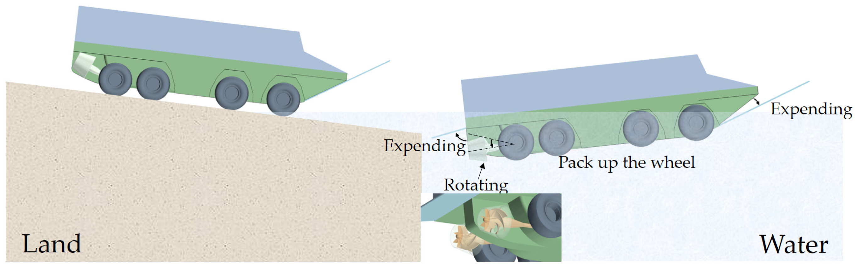[6] designed a wheeled amphibious truck with two rotatable carriages, where the carriages swivel into water to increase the amphibious vehicle’s displacement and seal the sides of the wheel wells. Therefore, the draft of the amphibious vehicle could be reduced and the flow field around wheel wells could be improved, both of which were beneficial for reducing the resistance of the amphibious vehicle.

Some scholars have carried out research on the wheel resistance characteristics. In 2007, Wu et al. [7] used steady methods to numerically simulate and analyze the resistance characteristics of a simplified wheeled amphibious vehicle model with a fixed attitude. By comparing the resistance difference between the amphibious vehicles when wheels were retracted and not retracted, they found that retracting wheels and closing wheel wells could reduce resistance by 40 percent. In 2020, Kang et al. [8] numerically simulated the resistance characteristics of a high-speed planing wheeled amphibious vehicle in three states, including no wheel retracted, front wheels retracted, and all wheels retracted. They indicated that retracting wheels could smooth out the streamlines at the vehicle’s bottom, which could effectively improve the flow field and reduce vortices. In addition, Zhou and Zhang [9] compared the resistance of amphibious vehicles with and without wheel openings and found that the resistance of amphibious vehicles with openings was greater. They proposed that retracting wheels and closing wheel wells could reduce vehicle resistance. At present, retracting wheels is one of the methods widely used in amphibious vehicles to reduce resistance. Some scholars have also carried out research on the retracting mechanism of wheels [10,11,12].

In general, there are many factors that affect the navigation resistance characteristics of the wheeled amphibious vehicles. The research on the resistance and improvement of wheeled amphibious vehicles mainly focuses on residual resistance. On the one hand, resistance improvement was achieved from the perspective of improving attitude, such as reducing the draft of amphibious vehicles by adopting planing vehicle body, lift wings and pontoons, such as optimizing the trim angle of amphibious vehicles by adjusting the angle of the bow breakwater and the stern flap [13,14,15,16]. On the other hand, resistance improvement was achieved by reducing the local shape resistance of amphibious vehicle part [17], such as reducing the negative effect of wheels on the resistance of amphibious vehicles by retracting the wheels. However, most of the current research on the wheel resistance characteristics is qualitative and lacks a quantitative basis, which are supplemented in this paper. In addition, the resistance improvement approaches for wheels are very simple. More resistance improvement approaches are proposed in this paper.

The research object of this paper is a medium-speed as well as heavy-load condition pump-jet-propelled wheeled amphibious vehicle (PJPWAV). Compared with conventional stern plate type waterjets, pump-jets have a higher propulsion efficiency at medium and low speeds. However, since pump-jets are completely submerged in water and the sufficient distance between pump-jets and vehicle body is required to avoid excessive thrust deduction, the PJPWAV usually reserve a considerable amount of space at the vehicle stern for the installation of the pump-jets. Therefore, compared with the conventional stern plate type waterjet-propelled wheeled amphibious vehicle (WJPWAV), the stern buoyancy of the PJPWAV is relatively smaller, the aft trim is more serious, and wheels are more strongly rushed by flow. By comparing the resistance components of wheeled amphibious vehicles using two propulsion forms under the same displacement and same working conditions, it is found that the proportion of wheel resistance in the total resistance of the PJPWAV is about twice that of the WJPWAV. Therefore, the resistance characteristics of wheels are more critical for the PJPWAV, and it is necessary to carry out further research on the resistance characteristics of wheels.

This study discusses the influence of wheels on total resistance for the PJPWAV. By decomposing the hydrodynamic effect of the wheels, the influence degree of each effect of the wheels is quantified, and the hydro-mechanism of each effect on total resistance is deeply explored. Finally, the corresponding resistance improvement approaches are proposed in a targeted manner, and the self-propulsion performance improvement effect of the resistance improvement model is also predicted.

2. Numerical Simulation

2.1. Geometry

The geometry of the PJPWAV studied in this paper was obtained by scaling the real amphibious vehicle, as shown in Figure 1. When the vehicle is driving on land, the bow breakwater and the stern flap are close to the vehicle body, and the pump-jets are lifted up by a certain angle through hydraulic mechanism, so that the vehicle has sufficient incidence angle and descent angle. When the vehicle is sailing in water, the bow breakwater and the stern flap are unfolded, the pump-jets are put down, and the wheels are retracted. It should be noted that the wheels are not fully integrated into the vehicle and the wheels protrude slightly relative to the vehicle’s bottom.

The main parameters of the PJPWAV model are listed in

Table 1. Main parameters of the amphibious vehicle mode.

Main Feature	Value
Overall length, L [m]	2.222
Overall beam, B [m]	0.707
Overall height, H [m]	0.687
The diameter of the wheel, Dw [m]	0.267

. The ratio of the length to the width of the PJPWAV is only 3.143, which is very small compared to conventional ships. In addition, the diameter of the wheels is very large, and the diameter sum for the four wheels can be close to half the length of the PJPWAV. The small ratio and the large diameter of the wheels are both one of the reasons for the great resistance on the PJPWAV.

The pump-jet of the PJPWAV consists of a 4-blade rotor and a 7-blade stator, as shown in Figure 2.

2.2. Numerical Set-Up

In the resistance prediction of bare vehicle, the PJPWAV without the pump-jet was used as the simulation model. Since the model is left-right symmetric, considering the cost of numerical simulation, only half of the model was simulated in this paper. Figure 3 shows the whole flow field domain and its boundary conditions. The inlet, bottom, top and sides are set as the velocity inlet, the outlet is set as the pressure outlet, the symmetry plane is set as symmetry, and the surface of the amphibious vehicle is set as the non-slip wall.

Reynolds-Averaged Navier–Stokes (RANS) equations were used to solve the computational domain. However, RANS equations are partial differential equations and cannot be solved directly. In the field of fluid mechanics, the finite difference method or finite volume method are usually used to transform partial differential equations into algebraic equations [18,19,20]. The details of the flow field can be approximatively obtained by using a computer to solve these algebraic equations. In this paper, the commercial software STAR-CCM+ was used to transform and solve the equations, where finite volume method was adopted. In addition, the SST k-w turbulence model with wall functions was applied [21,22]. The Volume of Fluid (VOF) method and the High-Resolution Interface Capturing (HRIC) format were used to capture the free surface [23,24,25]. The second-order upwind scheme was used to discrete the governing equations.

The motion of the vehicle was simulated by the dynamic fluid–body interaction (DFBI) model based on the technique of overset mesh. In order to improve the capture accuracy of the water surface, this paper set up three mesh refinement layers for the free surface and the Kelvin wave, respectively. The grid distribution of the computational domain is shown in Figure 4 and Figure 5.

As for the numerical simulation of the self-propelled vehicle, the flow field domain, boundary conditions, overset mesh setting, grid distribution, physical model and so on are basically the same as the bare vehicle model simulation. In particular, the additional mesh refinement was performed around the pump-jet in the self-propelled simulation. Moreover, the structured grid was used inside the pump-jet, as shown in Figure 6.

The rotation of the rotor was simulated using the multi-reference frame (MRF) method [26,27]. When the thrust of the pump-jet, T_p, satisfies Equation (1), it is considered that the amphibious vehicle model has reached the self-propulsion balance point [28].

$$T_p=R_t-F_D,$$

(1)

where F_D is the frictional resistance correction coefficient between the model and the actual vehicle. The definition of F_D is shown in Equation (2).

$$F_D=R_t-\frac{{\rho }_m}{{\rho }_s}\frac{R_{\mathit{t-s}}}{{\lambda }^3},$$

(2)

where R_t-s is the total resistance of the full-scale amphibious vehicle, λ is the scale ratio, and ρ_m and ρ_s are the density of the water in the model test and the real-scale test, respectively.

2.3. Uncertainty Analysis

In order to ensure the accuracy of the numerical simulation, this paper first conducted grid uncertainty analysis [29,30,31,32] for the resistance, sinkage and trim of the bare vehicle at design speed (Fr = 0.624). The grid numbers and simulation results of different mesh schemes are shown in

Table 2. The grid numbers and simulation results of three mesh schemes.

Mesh Schemes	Grid Numbers [Million]			Rt/∆ [-]		Sinkage/T [-]		Trim [deg]
	Back- Ground	Overset	Total	EFD	CFD	EFD	CFD	EFD	CFD
Coarse	46	125	171	0.275	0.291	−0.090	−0.119	−6.211	−6.161
Medium	103	243	346	0.275	0.282	−0.090	−0.103	−6.211	−6.168
Fine	223	459	682	0.275	0.281	−0.090	−0.099	−6.211	−6.172

, where R_t is the total resistance of the bare vehicle model; ∆ is the displacement of the amphibious vehicle model (unit is N); and T is the design draft of the amphibious vehicle model.

The verification factors of the uncertainty analysis of the bare vehicle are shown in

Table 3. Validation factors of the uncertainty analysis.

	RG [-]	CG [-]	UG [10−3]	E [%D]	UD [%D]	UV [%D]
Rt/∆	0.121	11.658	3.345	−2.336	3	3.237
Sinkage/T	0.197	6.923	10.650	−10.262	3	11.268
Trim	0.514	2.834	8.817	0.634	3	3.003

. Since 0 < R_G < 1, these three mesh schemes are monotonically convergent, and the mesh convergence is satisfied. Because |E| < U_V, the validation in these three mesh schemes is achieved. Considering simulation accuracy and cost, this paper chose the medium mesh scheme for subsequent research.

Figure 7 shows the numerical and experimental results of the bare vehicle model at 0.468 < Fr < 0.728. It can be seen that the R_t/∆ obtained by numerical simulation is slightly larger than the experimental value, but the deviation is within 6%; the trim is similar at high speed, but slightly deviates at low speed; the overall trends of sinkage obtained by the two methods are similar. On the whole, the numerical simulation results are in good agreement with the experimental results.

In addition, in order to verify the grid independence of the self-propelled simulation, three mesh schemes were set up in this paper. The grid numbers and numerical simulation results of these three mesh schemes are shown in

Table 4. The grid numbers and numerical simulation results of these three mesh schemes.

Mesh Scheme	Mesh Numbers [Million]					KT [-]	10KQ [-]
	Background	Overset	Rotor	Stator	Total
Coarse	45	209	73	90	417	0.418	0.734
Medium	103	409	146	185	843	0.406	0.699
Fine	234	818	296	369	1718	0.401	0.696

.

K_T and 10K_Q in Table 4 are the thrust coefficient and torque coefficient of the pump-jet, respectively, and their definitions are shown in Equations (3) and (4).

$$K_T=\frac{T_p}{\rho n^2{D}_p{}^4},$$

(3)

$$K_Q=\frac{Q_p}{\rho n^2{D}_p{}^5},$$

(4)

where Q_p is the torque of the pump-jet, ρ is the density of the water, n is the rotational speed, and D_p is the diameter of the rotor.

The R_G obtained from K_T and 10K_Q is 0.359 and 0.072, respectively, which are between 0 and 1. Therefore, the three mesh schemes are monotonically convergent, and the mesh convergence is satisfied. Considering simulation accuracy and cost, this paper chose the medium mesh scheme for subsequent self-propelled simulation.

3. Resistance Characteristics of the Amphibious Vehicle

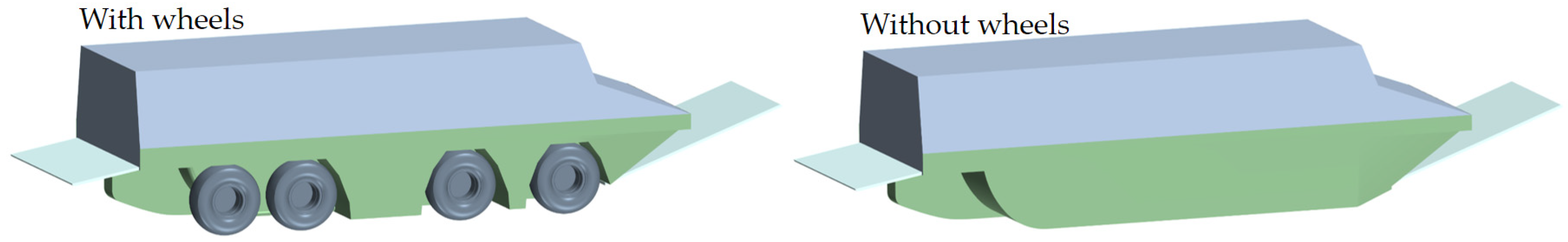
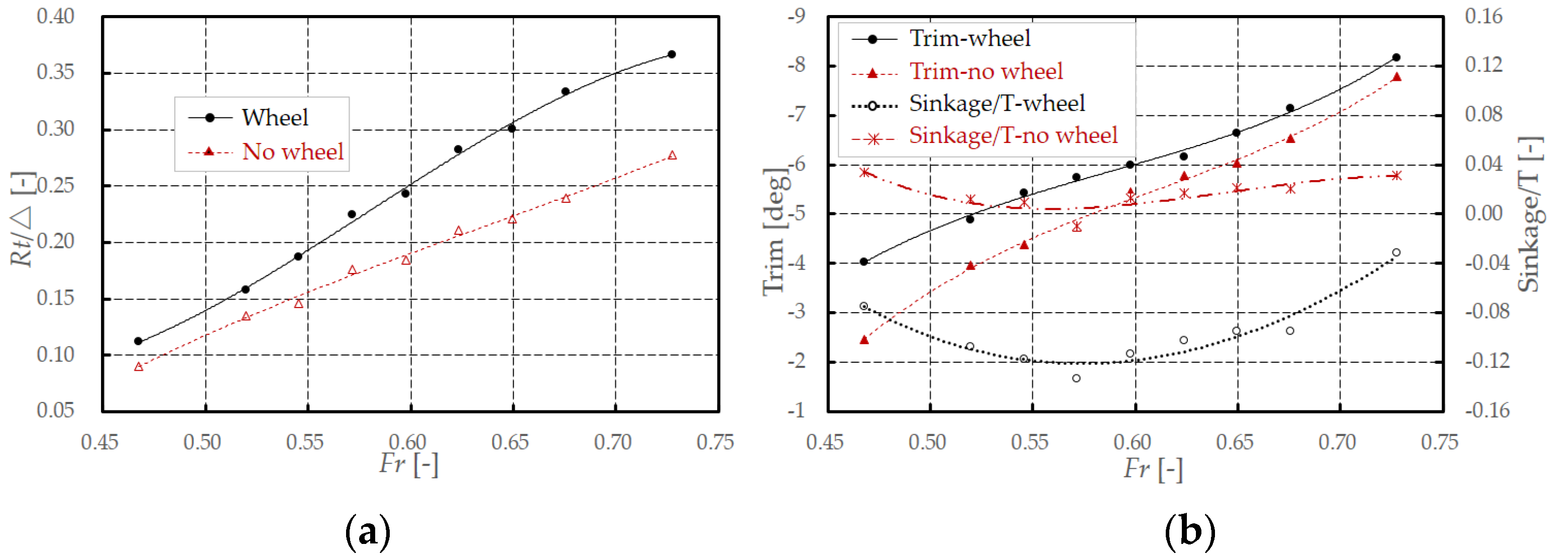
In order to understand the influence of the wheels on the resistance of the PJPWAV, this paper compared the resistance of the bare vehicle with and without wheels, as shown in Figure 8 and Figure 9. It can be seen that, under the influence of the wheels, the resistance of the amphibious vehicle increases significantly, and it becomes more obvious with the speed increase. At the same time, the draft and aft trim of the amphibious vehicle are also increased, and the change in draft is more obvious.

There are two reasons for the resistance variation caused by the wheels: the first reason is that installing the wheels changes the vehicle geometry; the second reason is that installing the wheels changes the vehicle attitude. The increased resistance due to geometric changes can be reduced by improving the local structure and flow field of the vehicle. The increased resistance due to attitude changes can be reduced from the perspective of adjusting attitude. By analyzing the influence and hydro-mechanism of each reason, the resistance improvement approaches can be proposed in a focused and targeted way, which is the basis for quickly and efficiently improving the resistance characteristics of the amphibious vehicle. Therefore, these two reasons need to be broken down and studied individually.

By comparing the amphibious vehicles with and without wheels, only the overall influence of two reasons can be obtained. This is insufficient for the intended study. In order to decompose these two reasons, this paper referred to the hull-waterjet interaction research method of waterjet propelled ships. 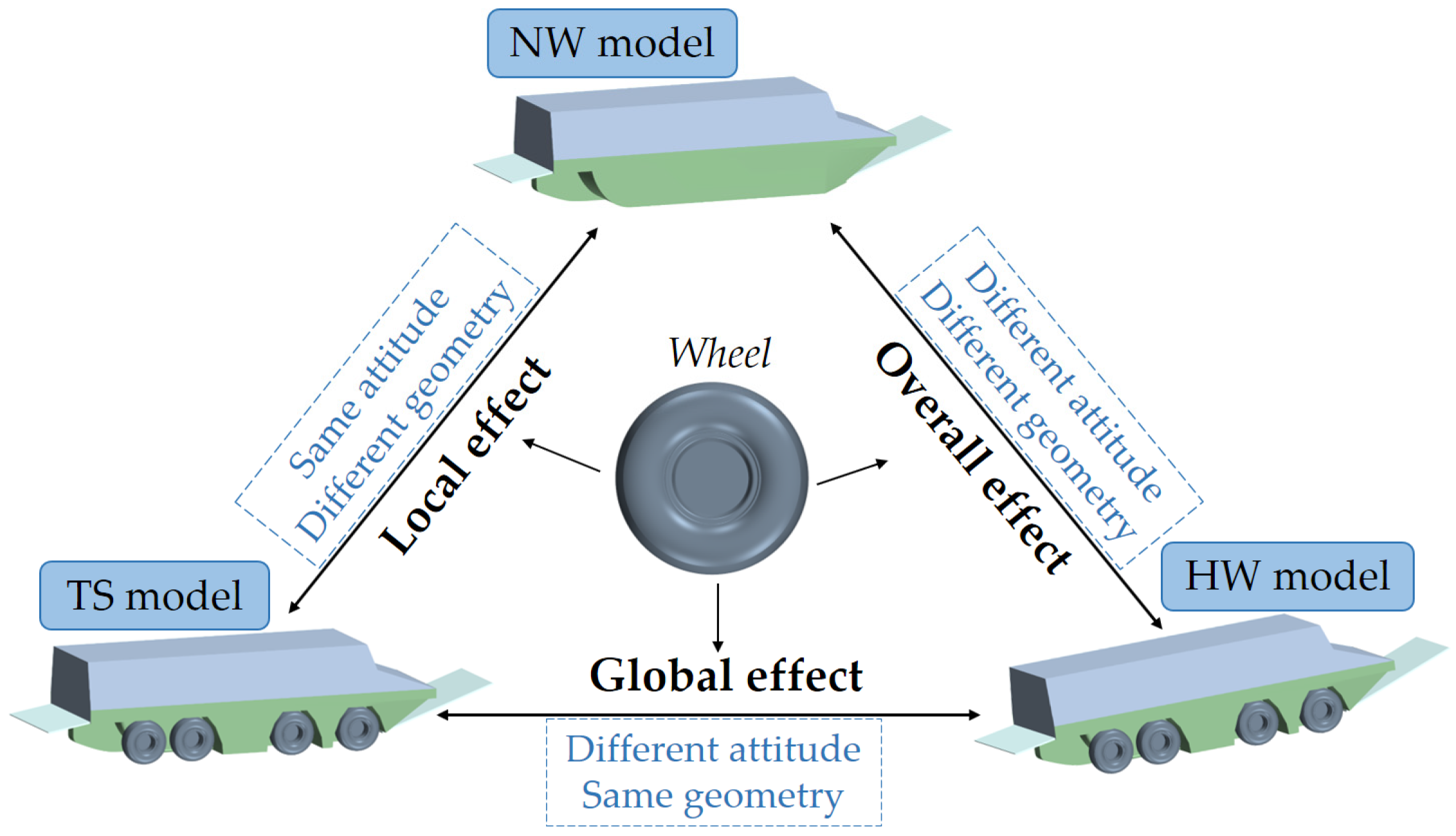This method proposed that there were two main reasons for the resistance increase caused by the waterjet: the first reason was the installation of the waterjet changed the hull geometry, and the suction as well as jet effect of the pump-jet changed the stern flow field; the second reason was the installation and operation of the waterjet changed the hull attitude [33,34,35,36]. This is very similar to studying the effect of the wheels on the resistance of the amphibious vehicles. This method referred to the first reason as the local effect and the second reason as the global effect and proposed a transitional hull model with the same geometry as the self-propelled hull (both with waterjet) and the same attitude as the bare hull. The resistance difference between the transition hull model and the bare hull was the local effect, and the resistance difference between the self-propelled hull and the transition hull model was the global effect.

According to this method, in this paper, the influence of the geometry change caused by the wheels on the resistance was called the local effect, and the influence of the attitude variation caused by the wheels on the resistance was called the global effect. In addition, a transition model with wheels was proposed, which has the same attitude as the amphibious vehicle without wheels. For the convenience of explanation, this paper called the amphibious vehicle model without wheels as the NW (No Wheels) model, the amphibious vehicle model with wheels as the HW (Have Wheels) model, and the newly proposed amphibious vehicle transition model as the TS (Transitional State) model. The relevant details can be seen in Figure 10. The attitude of the TS model is artificially constrained to be the same as the NW model.

In this study, K₁ and K₂ were used to describe the local effect and global effect, respectively. K₁ represents the resistance difference of the TS model relative to the NW model. K₂ represents the resistance difference of the HW model relative to the TS model. The definitions of K₁ and K₂ are shown in Equations (5) and (6):

$$K_1=\frac{R_{\mathit{t-TS}}-R_{\mathit{t-NW}}}{R_{\mathit{t-HW}}},$$

(5)

$$K_2=\frac{R_{\mathit{t-HW}}-R_{\mathit{t-TS}}}{R_{\mathit{t-HW}}},$$

(6)

where R_t-TS is the total resistance of the TS model; R_t-NW is the total resistance of the NW model; and R_t-HW is the total resistance of the HW model.

In addition, the resistance increment coefficient K was used to represent the overall effect of the wheels. K includes the local effect and the global effect, and its definition is shown in Equation (7).

$$K=K_1+K_2=\frac{R_{\mathit{t-HW}}-R_{\mathit{t-NW}}}{R_{\mathit{t-HW}}},$$

(7)

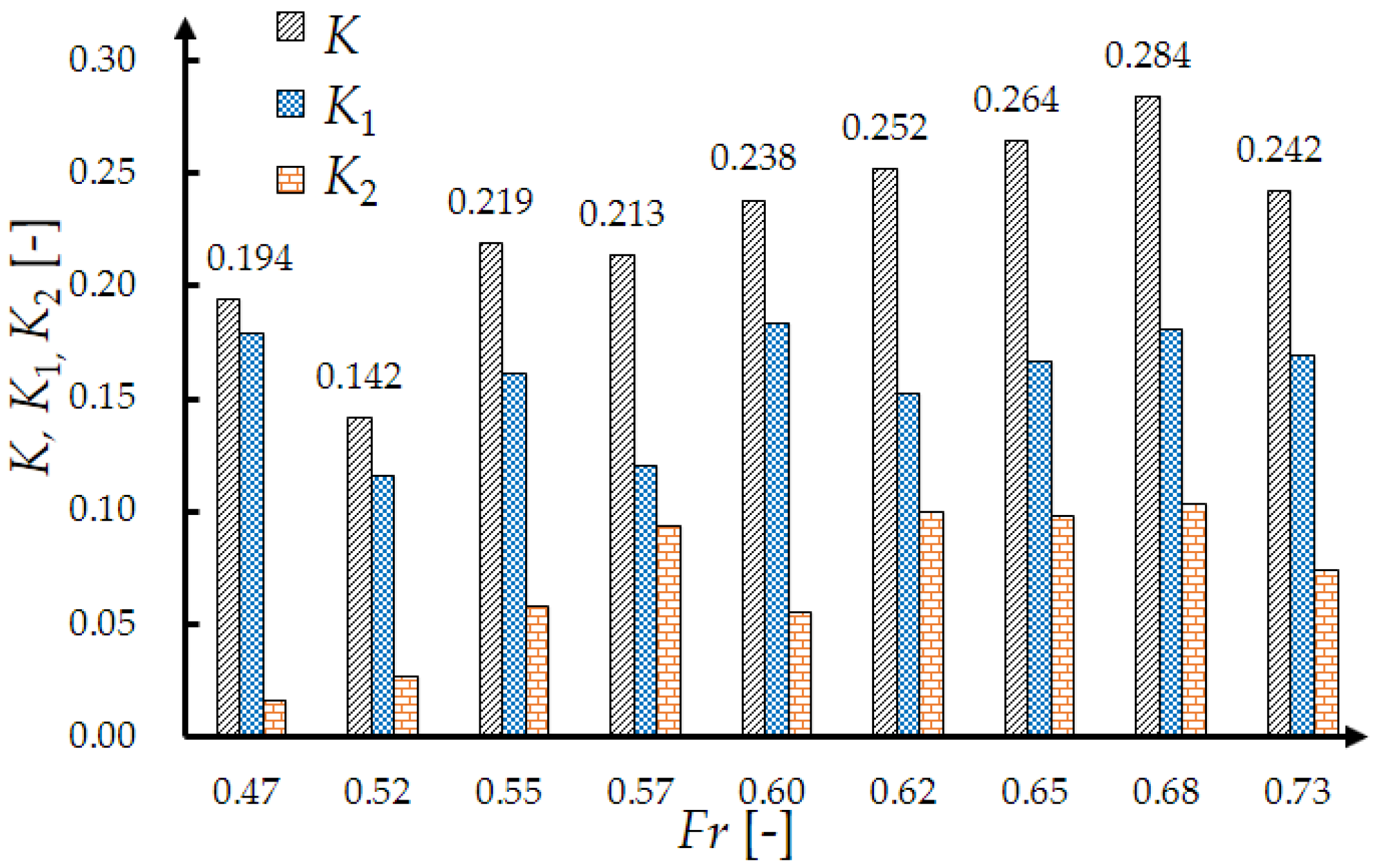
According to the same numerical simulation method to predict the resistance of the three models at various speeds, K₁, K₂, and K can be obtained, as shown in Figure 11.

At all simulated speeds, the resistance increment coefficient K is in the range of 0.142~0.284, and K reaches above 0.2 when 0.55 ≤ Fr ≤ 0.73, which indicates that the hydrodynamic effect of the wheels will increase the resistance of the amphibious vehicle by more than 20%. In addition, both K₁ and K₂ are positive, which represents that both the local effect and global effect of the wheels increase the resistance of the amphibious vehicle. It should be noted that K₁ is significantly larger than K₂ at each speed. Therefore, the local effect of the wheels has a more significant effect on the resistance of the amphibious vehicle than the global effect. In order to quickly and efficiently propose resistance improvement approaches, this paper analyzed the hydro-mechanism of K₁ in detail, and briefly analyzed the reasons why K₂ affects the resistance of the amphibious vehicle.

3.1. The Local Effect K₁

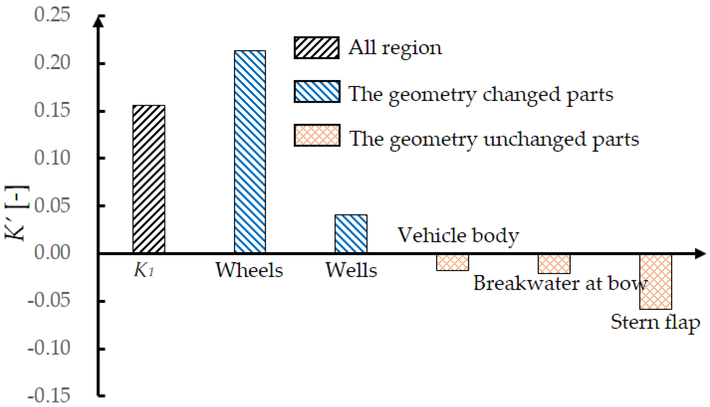
In order to clarify the hydro-mechanism of the local effect K₁, this paper divided the vehicle body into two parts, including the geometry changed parts and the geometry unchanged parts, and discussed them separately. The geometry changed parts include the wheels and wheel wells. The geometry unchanged parts include the bow breakwater, the stern flap, and the vehicle body outside the wheel wells. Figure 12 shows the effect of the two parts.

K’ in Figure 12 represents the resistance variation of vehicle parts, and its definition is shown in Equation (8).

$$K^{\prime }=\frac{\delta R_{Part}}{R_{\mathit{t-HW}}},$$

(8)

where δR_Part is the part resistance difference between the TS model and the NW model.

It can be seen from Figure 12 that the resistance of the geometry changed parts increases, and the resistance of the geometry unchanged parts decreases. The reasons for the resistance variation of each part will be discussed in detail below.

3.1.1. The Geometry Changed Parts

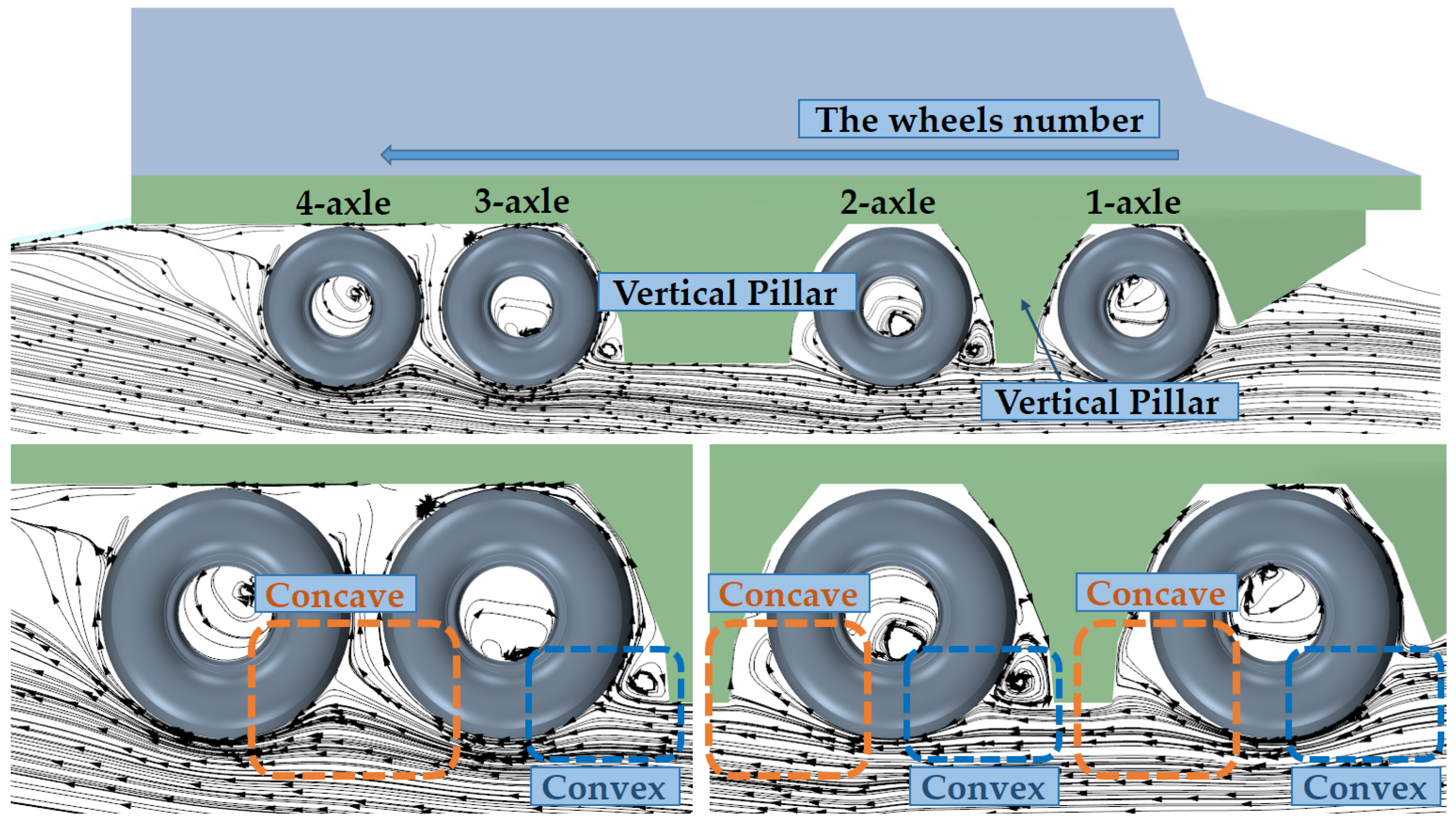
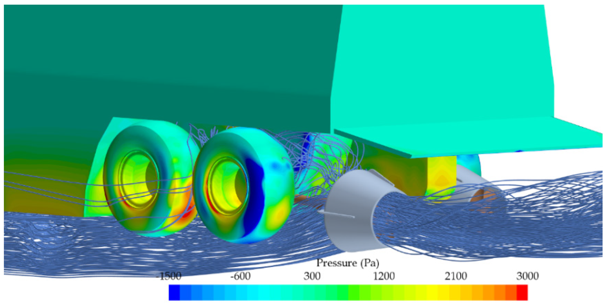
The wheels and wheel wells of the amphibious vehicle in this paper are large in size and many in number, which promotes the formation of convex and concave structures at the bottom of the wheel longitudinal section. These convex and concave structures prevent the flow from passing smoothly along the vehicle bottom, which causes the flow to violently rush the wheels and wheel wells, as shown in Figure 13.

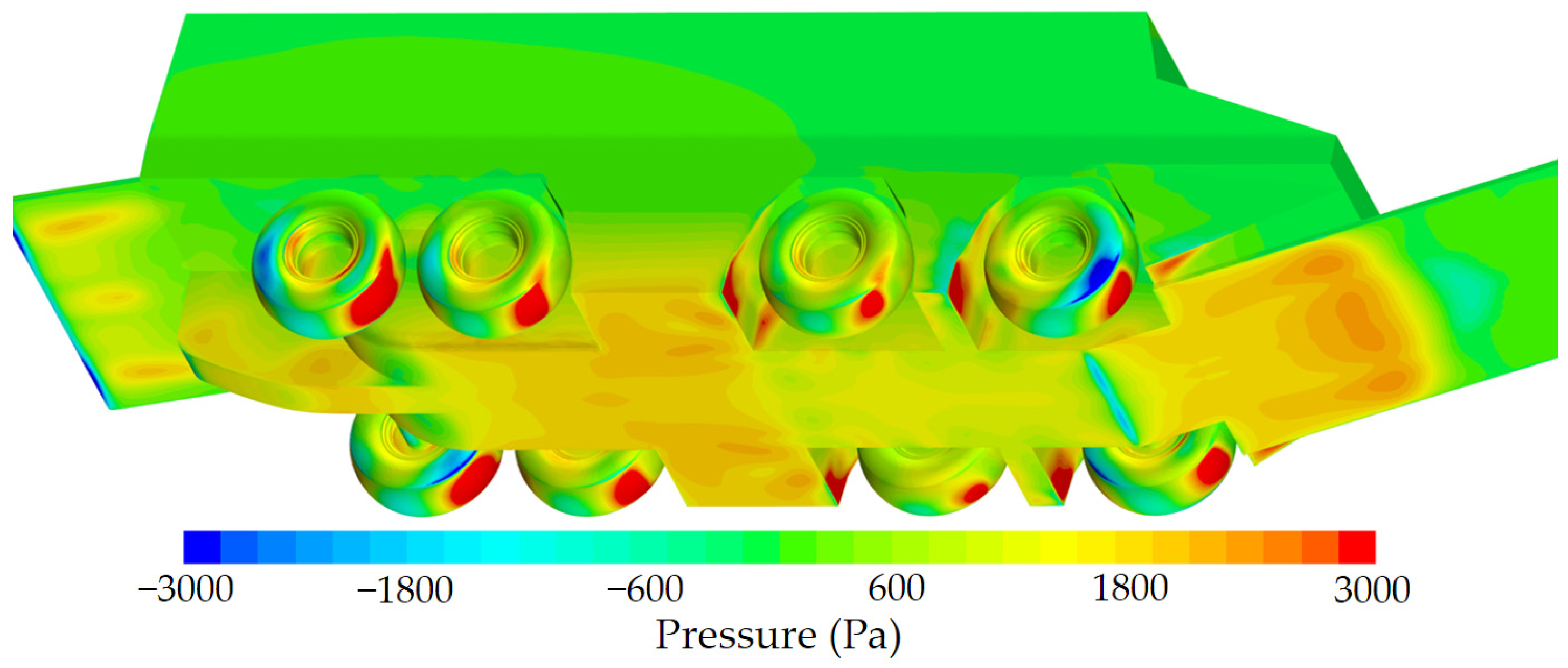
Under the rush of flow, the wheels and wheel wells form a large number of obvious high-pressure areas, which is one of the main reasons for the high resistance of the wheels and wheel wells, as shown in Figure 14.

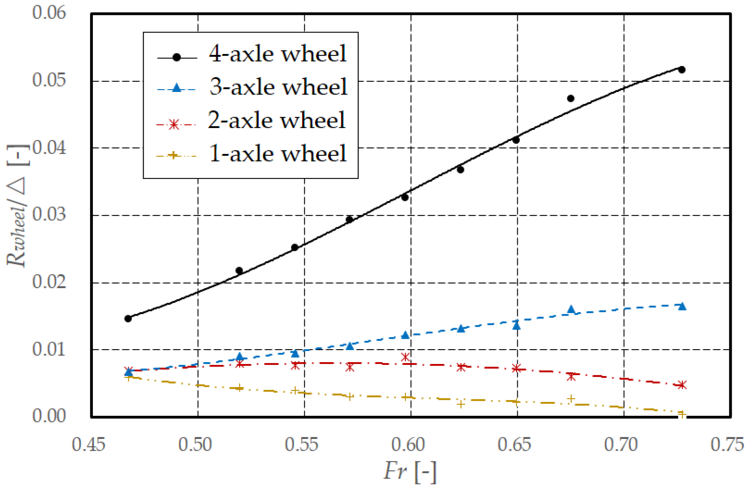
In detail, the front half convex structures of the 1-axle, 2-axle, and 3-axle wheels are rushed by the flow along the vehicle bottom, and thus put under high pressure. The contour of the rear half of the wheels gradually shrinks along the flow direction, forming a relatively obvious diffused concave area, which induces the flow to turn along the wheel contour. For 1-axle and 2-axle wheels, part of the flow after turning rushes to the wheel wells, forming obvious high pressure, and the other part continues to flow to the next axle wheels along the vehicle bottom. For the 3-axle wheels, since there is no vertical pillar between the 3-axle wheels and the 4-axle wheels (refer to Figure 13), most of the flow after turning rushes the 4-axle wheels. As a result, the 4-axle wheels have a large area of high-pressure region, which causes the resistance of the 4-axle wheels to be much greater than that of the other three axle wheels, as shown in Figure 15. It can be seen from the above that reducing the high pressure of the wheels and wheel wells may be a very effective resistance improvement approach, especially for 4-axle wheels.

3.1.2. The Geometry Unchanged Parts

The influence of the wheels and wheel wells on the flow field around themselves will also change the forces on the geometry unchanged parts. As shown in Figure 12, under the local effect of the wheels, the resistance of the bow breakwater and the vehicle body decreased slightly, and the resistance of the stern flap decreased significantly. On the one hand, the installation of wheels decreases the smoothness of the amphibious vehicle, reduces the velocity of the flow field around the vehicle body, and weakens the rush of the flow on the geometry unchanged parts. On the other hand, the flow field will also have special change due to some structural changes, especially in the stern flap. As shown in Figure 16, there is a beam of high-speed streamlines rushing the stern flap of the NW model. In the TS model, because the wheels change the direction and speed of the stern streamline, there is no streamline that violently rushes the stern flap.

Obviously, the resistance reduction of the vehicle body, the bow breakwater and the stern flap is beneficial to the total resistance of the amphibious vehicle. One of the methods to further improve the resistance of the amphibious vehicle is to propose measures that can increase the magnitude of the resistance reduction. However, this is a very complex problem and difficult to achieve.

3.2. The Global Effect K₂

The global effect K₂ accounts for a relatively small proportion of the total effect K, which is caused by the vehicle attitude variation. K₂ represents the resistance difference between the HW model and the TS model. The attitude of the TS model is constrained to be the same as the NW model, and the attitude difference between the HW model and the TS model is shown in Figure 9. Under the effect of the wheels, the draft of the amphibious vehicle has been increased by a relatively large margin, and the aft trim is slightly increased.

From the perspective of static lift, when the amphibious vehicle sails in water, the gap between the wheels and the wheel wells is filled by water, and thus the buoyancy of the NW model will be lost, which in turn causes the vehicle body to sink. However, since these four axle wheels are approximately symmetrically distributed in the front and rear of the gravity center, the moment formed by the buoyancy loss relative to the gravity center is very small, and thus the aft trim of the amphibious vehicle has only changed slightly.

The increase in draft and aft trim will increase the vertical projection area of the vehicle body to cut off the flow, which will strengthen the blocking effect of the vehicle body on the flow. Therefore, for the global effect of the wheels, reducing the buoyancy loss between the wheels and the wheel wells is an effective measure to reduce the resistance.

4. Research on the Resistance Improvement of the Amphibious Vehicle

It can be seen from the above analysis that the hydrodynamic effect of the wheels will significantly increase the resistance of the amphibious vehicle. In order to reduce the negative effect of the wheels, one of the most effective measures is to turn the amphibious vehicle model into the NW model of this paper, for example, the wheels are completely retracted and the wheel wells are sealed with flat plates. This measure can completely eliminate the effect of the wheels, but it is difficult to achieve in engineering. Therefore, according to the effect mechanism of the wheels on resistance, this paper proposes the less difficult resistance improvement approaches to be realized in engineering.

4.1. Increasing Wheel Retraction

In the local effect of the wheels, the main reason for the resistance increase is that the longitudinal convex and concave structures formed by the wheels and the wheel wells cause an obvious high-pressure area in the wheels and the wheel wells. As for the global effect of the wheels, the main reasons for the resistance increase are: the gap between the wheels and the wheel wells causes a lot of buoyancy loss, which makes the vehicle body sink and aft trim larger, and thus the blocking effect of the amphibious vehicle on flow has also become stronger.

For the local effect of the wheels, the wheels should be retracted until the wheel bottom is flush with the vehicle bottom, which can weaken the convex and concave. As for the global effect of the wheels, the vehicle structure should be made more compact, which can reduce gap and buoyancy loss.

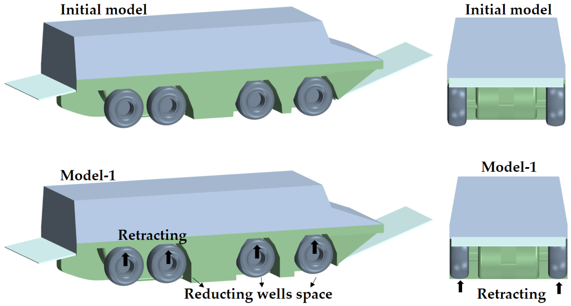
Based on the above analysis, the resistance improvement Model-1 is obtained by increasing wheel retraction and reducing the gap between the wheels and the wheel wells, as shown in Figure 17. However, because the gap reduction is very small, the resistance improvement is mainly contributed by increasing wheel retraction.

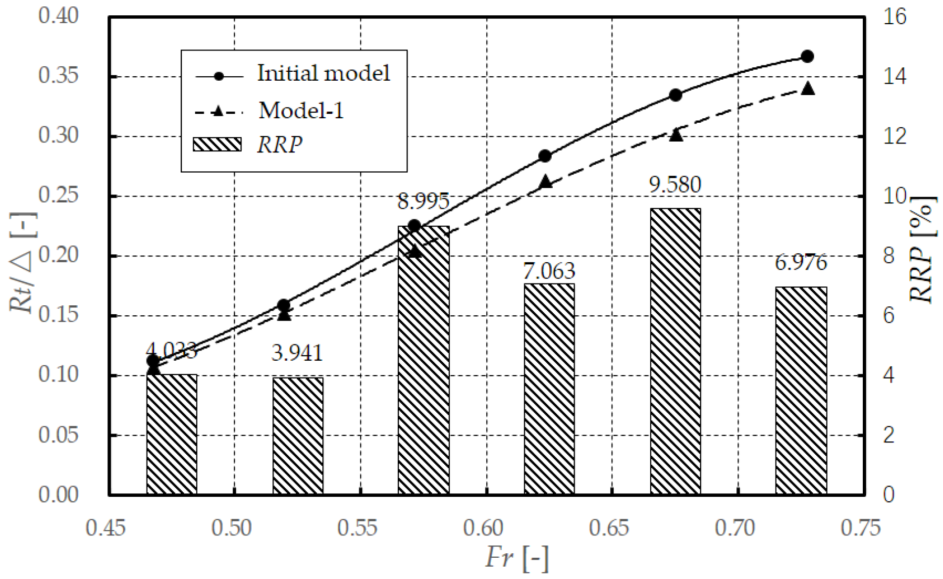
The resistance of the initial model and the Model-1 at various speeds are shown in Figure 18. The RRP of Figure 18 represents the resistance reduction percentage of the Model-1 relative to the initial model. It can be seen from it that, compared with the initial model, the Model-1 has less resistance at each speed. In detail, when 0.468 < Fr < 0.520, increasing wheel retraction can reduce the resistance by about 4%, and when 0.572 < Fr < 0.728, the resistance reduction effect is better, which can reach more than 6.9%.

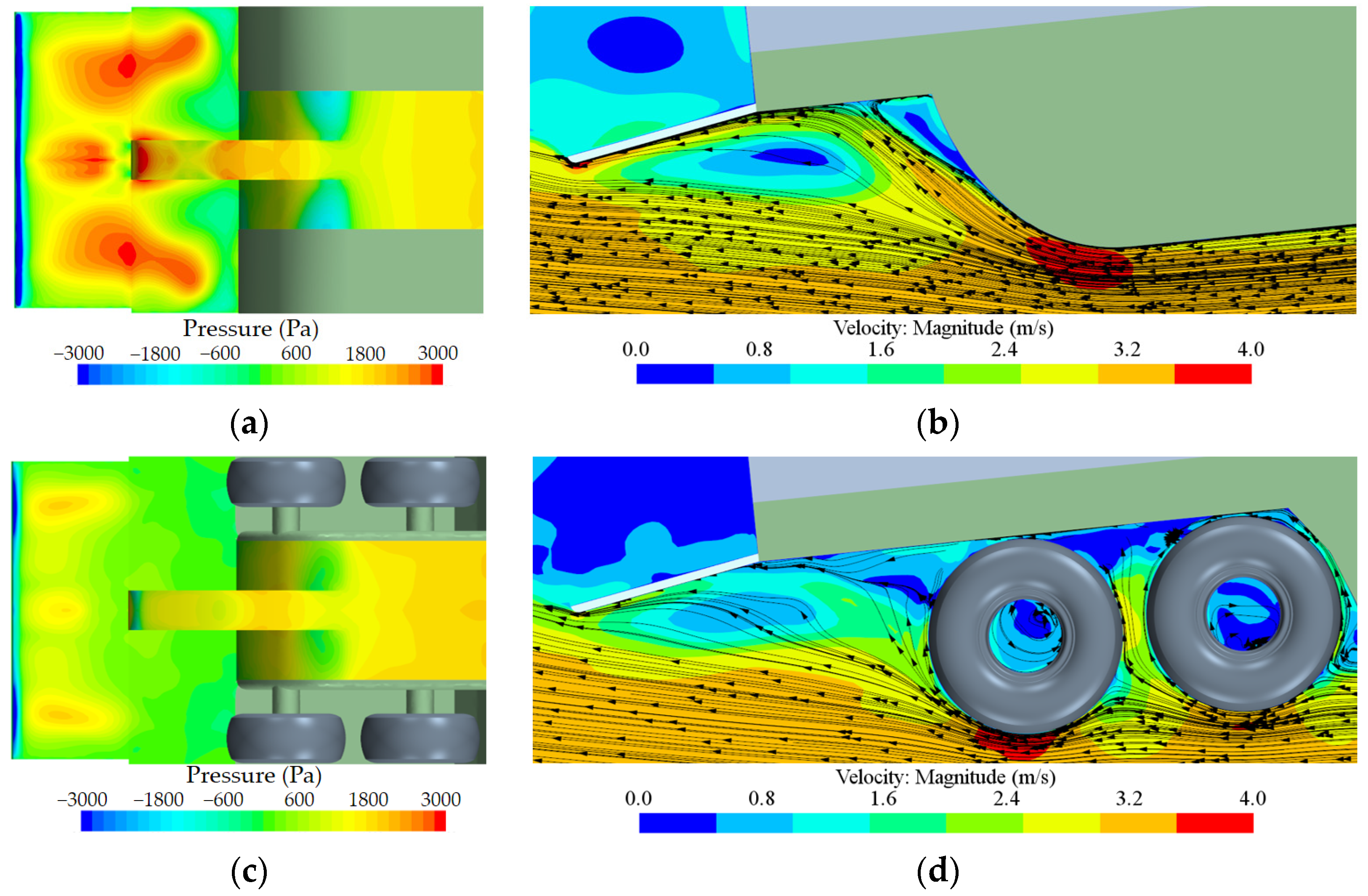
Figure 19 shows the streamline and pressure distribution at the wheel longitudinal section of the initial model and the Model-1, respectively. It can be seen that, after the wheel retraction is increased, the flow at the vehicle bottom can pass through the wheels more smoothly, the pressure in the wheel convex area is significantly reduced, and the pressure in the concave area also decreases slightly.

4.2. Installing Flat Plates on the Wheel Well Bottom

As Figure 19 shows, after the wheels are completely retracted, the flow in the concave region is still deflected along the wheel contour and continue to rush the next axle wheels and wheel wells, so that some high-pressure areas still exist. In order to reduce the high pressure in the concave region, this paper attempted to install flat plates on the wheel well bottom to improve the flow direction, so as to prevent the flow from hitting the wheel wells or wheels.

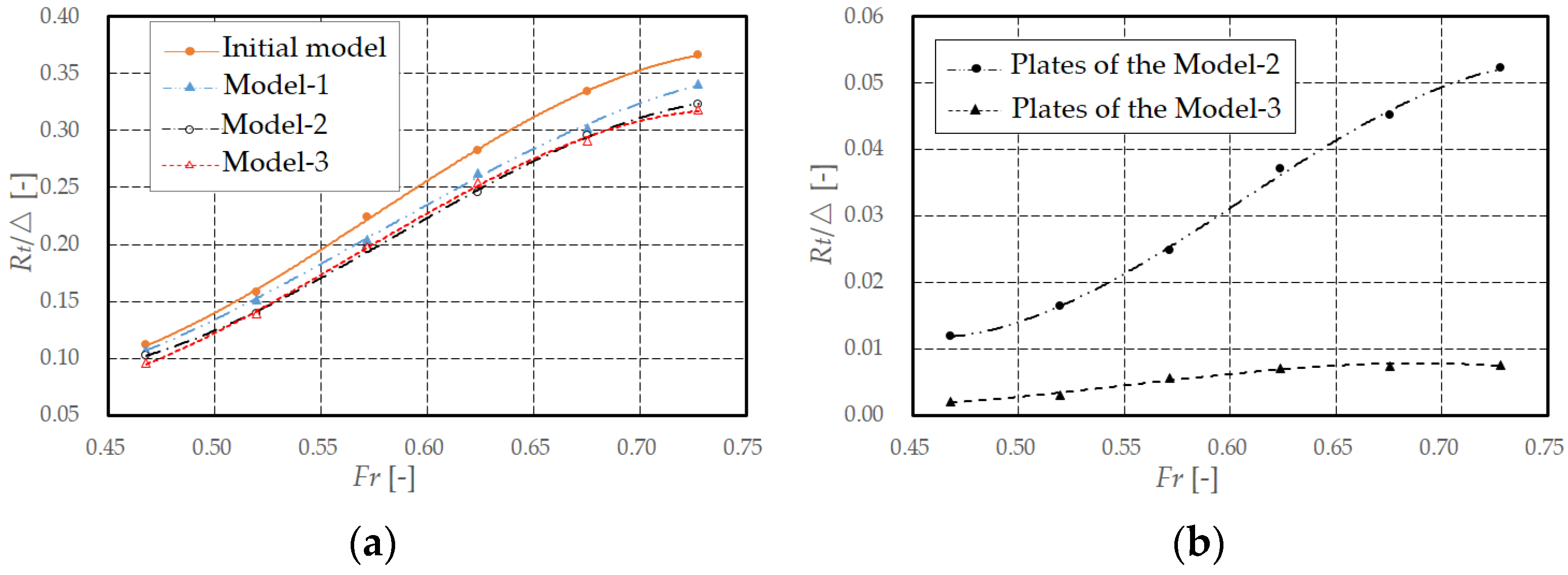
On the basis of the Model-1, this paper proposes two other resistance improvement models by installing flat plates on the wheel well bottom, as shown in Figure 20. In the resistance improvement Model-2, the bottoms of all wheel wells are completely enclosed with flat plates. The resistance improvement Model-3 is only aimed at the 4-axle wheel wells with the most obvious high pressure, where a small flat plate is installed on the bottom of the 3-axle and 4-axle wheel wells.

The streamline and pressure distribution of the resistance improvement models are shown in Figure 21 and Figure 22, respectively. Installing flat plates on the wheel well bottom allows water to flow more smoothly along the vehicle bottom. In detail, the 1-axle and 2-axle wheel wells can effectively reduce their own high pressure by installing the flat plates on the wheel well bottom, which is beneficial to reduce the resistance of the 1-axle and 2-axle wheel wells. Completely closing the bottom of the 3-axle and 4-axle wheel wells (Model-2), or only installing a small plate on the bottom of the 3-axle and 4-axle wheel wells (Model-3) can both effectively reduce the high pressure at the 4-axle wheels, which can reduce the resistance of the 4-axle wheels by 65.6% or 64.7%, respectively (at Fr = 0.624)

However, while the flat plates improve the resistance of wheels and wheel wells, the flat plates are experiencing resistance. Moreover, the resistance of the flap plates will increase with the plate area increase. The resistance of the resistance improvement models as well as the flap plates are shown in Figure 23. Although the pressure reduction in Model-2 is more significant than that of Model-3, the overall resistance improvement effect has no obvious advantage due to the greater plate resistance.

From the perspective of the total resistance of the amphibious vehicle, installing flat plates on the concave region of the vehicle bottom does not always have a good resistance improvement effect. In this paper, installing a small plate on the bottom of the 3-axle and 4-axle wheel wheels can significantly reduce the total resistance, but installing the plates on other places had only little effect. Installing the flat plates without resistance improvement effect will increase the manufacturing difficulty in vain. Therefore, before installing the flap plates, the resistance characteristics of the amphibious vehicle and the effect mechanism of the wheels should be analyzed. Furthermore, the resistance improvement, the resistance of the flap plates, and the manufacturing difficulty as well as cost should be comprehensively considered.

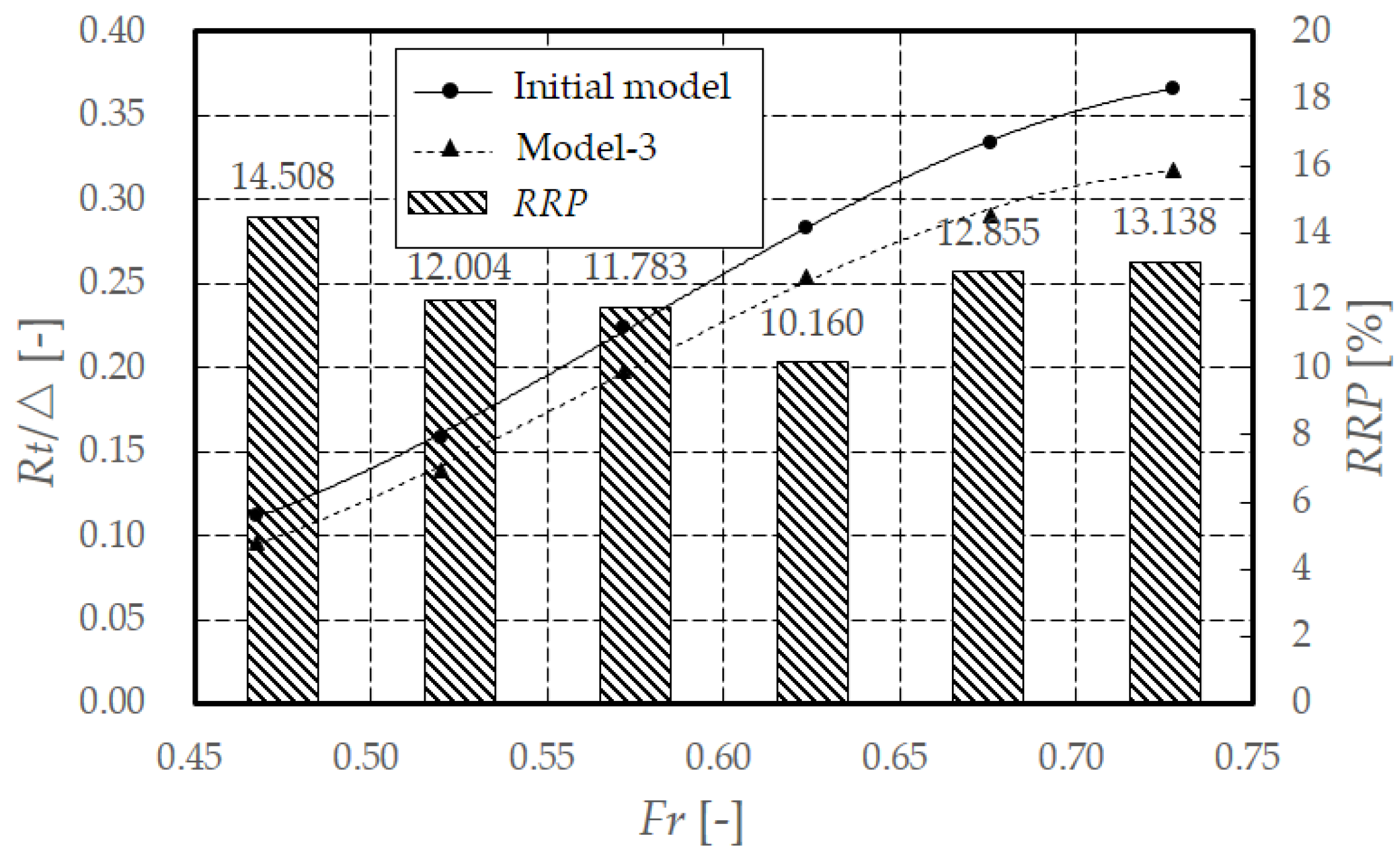
Considering the resistance improvement effect and installation difficulty of the flap plates, the Model-3 was selected as the ultimate resistance improvement model in this paper. The resistance predictions for the Model-3 at other speeds are supplemented, as shown in Figure 24. The RRP of Figure 24 represents the resistance reduction percentage of the Model-3 relative to the initial model. As can be seen, compared to the initial model, the Model-3 reduces resistance by no less than 10% at design speed (Fr = 0.624) and by an average of no less than 12% at all simulated speeds. In addition, as shown in Figure 18 and Figure 24, by comparing the resistance of the Model-2 and the Model-3, it can be found that when 0.468 < Fr < 0.520, installing a flat plate at the bottom of the 3-axle and 4-axle wheel wells has a good resistance improvement effect, and the resistance reduction can reach 8~10.4%; when 0.572 < Fr < 0.572, this approach can reduce the resistance by 2.8~6.1%.

5. Self-Propelled Characteristics of the Amphibious Vehicle

In order to explore the improvement effect of the resistance improvement approaches on self-propulsion performance of the amphibious vehicle, this paper numerically simulated the self-propulsion performance of the initial model and Model-3 under the design speed (Fr = 0.624). The characteristics of the amphibious vehicle sailing at Fr = 0.624 are shown in

Table 5. Self-propelled characteristics of the initial model and Model-3 at Fr = 0.624.

	Fr [-]	n [-]	Rself/∆ [-]	P [-]	η [%]
Initial model	0.624	n0	0.327	P0	42.061
Model-3	0.624	0.983 n0	0.287	0.914 P0	41.327

.

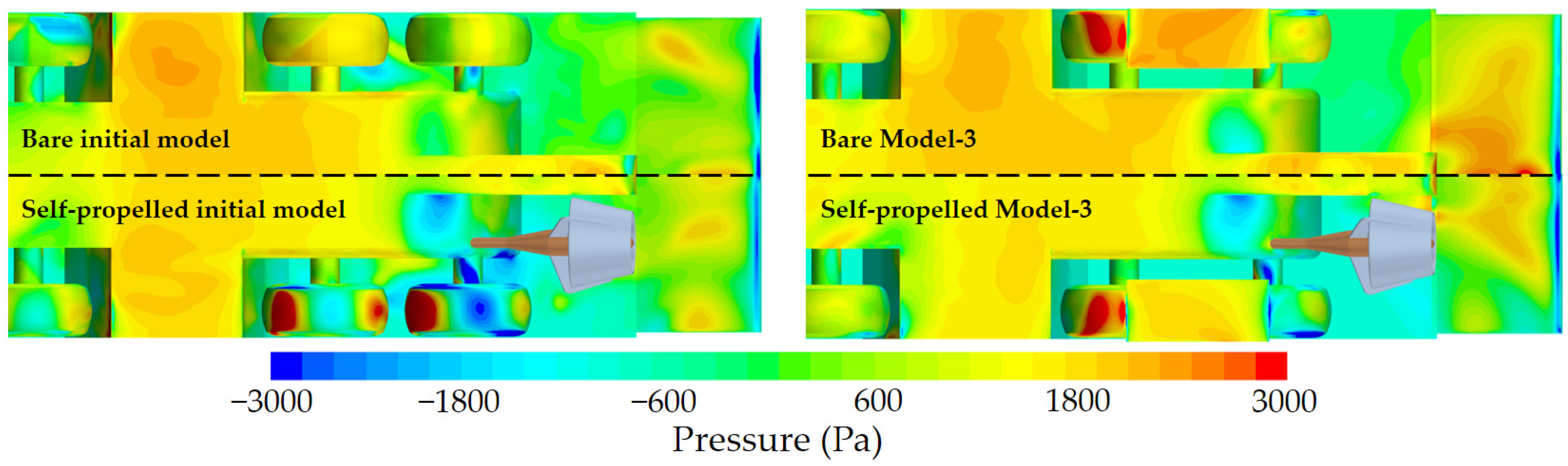
As can be seen from Table 5, the rotational speed n and the self-propelled resistance R_self of the pump-jets of the Model-3 relative to the initial model decreased by 1.741%, and 12.325%, respectively. In addition, it is very important that the Model-3 saves 8.564% of the power compared to the initial model at the design speed. This means that the self-propulsion performance of the amphibious vehicle has been significantly improved. There are two main reasons why the Model-3 requires less power. The first reason is that the Model-3 has less resistance on the bare vehicle. Moreover, for the self-propelled vehicle, due to the stern limited space, the suction flow of the pump-jet is very close to the stern ve-hicle body, as shown in Figure 25.

The pressure of the vehicle stern drops significantly under the suction of the pump-jet, which increases the resistance of the amphibious vehicle, as shown in Figure 26. Because the rotating speed of the Model-3 propeller is relatively smaller, its pressure reduction of the vehicle stern is smaller in the self-propelled state. Therefore, the second reason is that the Model-3 requires less rotating speed, which results in a smaller re-sistance increase caused by the pump-jets.

The propulsion efficiency η of the Model-3 is slightly reduced relative to the initial model, mainly because the power consumed by the pump-jets is much reduced. However, the propulsion efficiency of the pump-jets is still much higher than conventional stern plate type waterjets. From the above analysis, it can be seen that the resistance improve-ment approaches proposed in this paper have a good resistance and propulsion perfor-mance improvement effect.

6. Conclusions

(1).

For the pump-jet-propelled wheeled amphibious vehicle, the resistance of the amphibious vehicle is increased by 14~28% under the hydrodynamic effect of the wheels at 0.468 < Fr < 0.728. In detail, the local effect of the wheels has made a great contribution, which is mainly manifested in that the longitudinal convex and concave structures formed by the wheels and the wheel wells guide the flow to rush on the wheels and the wheel wells, forming high pressure and great resistance.

(2).

Increasing wheel retraction and installing flap plates on the wheel well bottom can weaken the convex and concave, which can reduce the resistance of the amphibious vehicle. However, the plates are also experiencing resistance, which will counteract the resistance improvement. Therefore, the resistance improvement, the resistance of the flap plates, and the manufacturing difficulty as well as cost should be comprehensively considered before installing plates.

(3).

The gap between the wheels and the wheel wells causes a lot of buoyancy loss, which makes the vehicle body sink and aft trim larger, and thus the blocking effect of the amphibious vehicle on flow has also become stronger. This is one of the reasons why the resistance of amphibious vehicles increases. Therefore, in order to reduce the gap between the wheels and the wheel wells, the amphibious vehicle should be designed as compact as possible.

(4).

At the design speed (Fr = 0.624), the ultimate resistance improvement model proposed in this paper can reduce the resistance by no less than 10% and save the power by no less than 8%. The resistance and propulsion performance of the PJPWAV were significantly improved.