Experimental and Numerical Resistance Analysis for a Cruise Ship W/O Fin Stabilizers

Abstract

Applying fin stabilizers is an effective solution for ship rolls on waves in a seaway. They generally consist of one or two pairs of retractable fins that are symmetrically mounted to both sides of the ship, effectively reducing the roll motion at low or moderate speeds. Fin stabilizers are commonly used by cruise ships for the comfort and safety of passengers. However, there is still little experimental and numerical analysis of the fins’ effect on hydrodynamic performance. In this study, the resistance performance of a cruise ship was investigated with/without fin stabilizers at different fin angles and ship velocities by model tests and numerical analysis. The CFD analysis provides a flow-detailed interpretation of the physical phenomenon, especially at an asymmetric maximum fin angle. The significant fin-induced resistance is newly discovered and averages up to 19% in calm water conditions, while the added resistance in waves is evaluated with a smaller increment up to 1.31%. By comparing the numerical and experimental results, this study provides insight into the resistance induced by overhanging fins, which provides an accurate prediction reference for cruise ship performance and benefits the fin stabilizers’ design and selection.

1. Introduction

Fin stabilizers, normally a pair or two, are anti-roll devices located below the water line on both bilge sides of a ship hull to resist the rolling motion of a seaway. With a long development history, they are commonly used by various ships, such as cruise ships, to provide comfort and safety to passengers. Many researchers have investigated general stabilizers, such as the rolling tank [1], moving weight [2], gyroscope [3], and bilge keel [4,5], which stabilize the ship’s roll motion at a low ship speed. However, obstacles include their large size, power, or cost demands [6].

A pair of fin stabilizers usually consists of two fins with hydraulic power units and local control units (LCU), one bridge control panel (BCP), a main control unit (MCU), and a roll motion sensor unit (RMSU) [7], as shown in Figure 1.

A procedure was provided for selecting and evaluating the ship roll stabilization systems, including passive tank, bilge keels, activated fins, and rudder roll stabilizers [8].

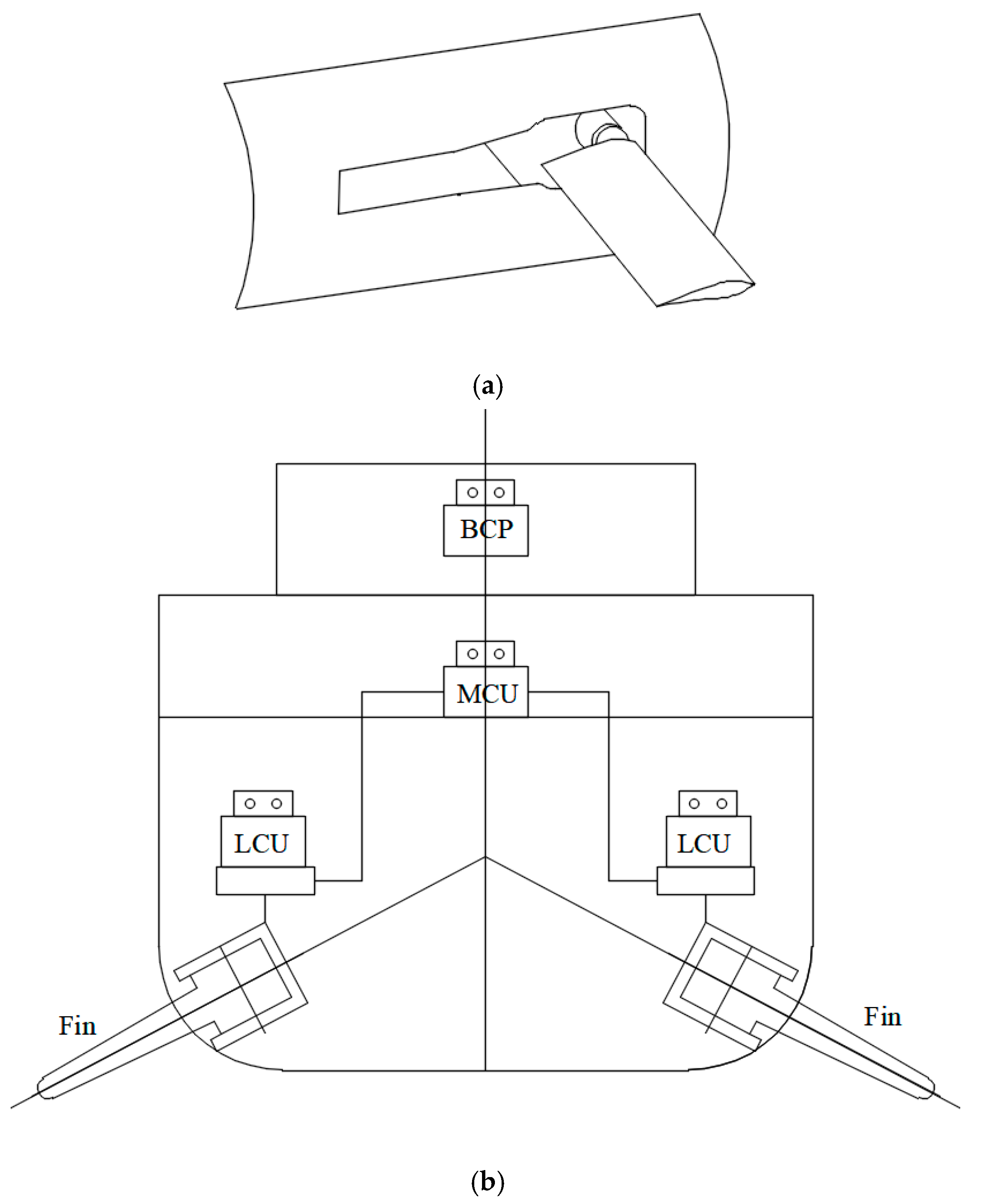
1.1. Review of the Fin Stabilizers Development

MARIN investigated the steady and unsteady performance of the fin hydrofoil while three different ships with fin stabilizers underwent a model test and numerical calculation for fin lift and drag characteristics [9,10]. Consideration has been made for a constraint on the effective angle of attachment to prevent dynamic stall [11].

From the resistance point of view, the with/without (W/O) status of the fin stabilizers is a matter attracting researchers’ attention. The numerical analysis of the fin’s resistance and bare hull with/without fins was computed and compared to the towing tank data [12]. A resistance model test and numerical simulations were conducted on a container ship with fins located at the forebody [13]. However, only small angles at 5° and 10° were investigated. For a 1412 t displacement yacht, the resistance with fins increased by about 6% compared to that without fins [14]. The ship resistance of fin stabilizers with NACA 0013 hydrofoil on patrol boats with angles of 0°, 5°, 10°, and 15° and speed variations of 25–30 kn was calculated with the CFD tool; the drag increased due to the rise in the fins’ angles. At an angle of 15°, the increments were 13.92–18.79% of the total drag of the ship [15].

In conclusion, previous research has demonstrated that with a fin angle of 0°, the ship resistance is <2%, and at an attack angle of 15°, it is 17.5%. However, few experimental verifications for the fin stabilizer influence the resistance performance of overhang fins.

The fin stabilizer is the most used anti-rolling device for ships nowadays and is only considered for its good stabilization effect at moderate speed. It is difficult to generate sufficient lift for efficient roll reduction at lower speeds. The best way to resolve this problem is to improve the conventional fin stabilizer to have an anti-rolling ability at all ranges of speeds; this improved version is called the zero-speed fin stabilizer [16]. Unlike the conventional fin rotation along the wing section axis to provide lift, at zero speed there is another “paddle” mode for providing larger lift, which is rotation along the chord-wise axis, with a small aspect ratio and an eccentric shaft position [17]. A pair of fin stabilizers was used to generate the anti-rolling force to reduce the ship’s roll motion at zero speed using the paddle principle.

Recently, research on novel stabilizers such as high-lift fin [18,19] and Magnus stabilizers has emerged [20,21]. The former is based on bionics principles. One of the high-lift fins has the application of the proper amount of bump shapes at the leading edge of the fin, while the morphing humpback fin can provide more lifting force at a small angle of attack [18]. Another factor is the variable area of parallelogram fin stabilizers, which had a 50% higher increase in lifting force than conventional rectangle fin stabilizers at zero speed [19]. The latter is a novel device for the anti-rolling of ships, which generates lift through a high-speed rotating rotor (rotor wing) based on the Magnus effect.

Although fin stabilizer technology has been applied to marine ships, cruise ships are different from other ships due to their high safety and comfort requirements during the voyage. It is particularly critical to customize the fin stabilizer to the specific parameters of the cruise ships to avoid excessively high resistance to the cruise ship when stretching for maximizing the rolling stabilization [22]. Generally, with a passenger capacity above 5000 people, the Oasis-class cruise ships mainly adopt fin stabilizers to keep the ship stable [23].

The parametric roll motion of a cruise ship with 500,000 t displacement and fin stabilizers was investigated in fin gains and aspect ratio [24]. A numerical analysis of the wave-induced motion of a cruise ship with stabilizing fins was conducted [25].

When the ship’s speed is 23 kn (moderate speed), the roll amplitude of the controlled system is reduced by 90.1%. When the ship’s speed is 7 kn (low speed), the roll amplitude is reduced by 52.3% [26].

1.2. Current Work

Although there has been plenty of research in academic reviews on fin resistance evaluation, the resistance caused by the fins at different angles with various speeds lacks investigation. Some research focuses on lift and drag force characteristics for the fin stabilizers; however, the validation of the computations is insufficient, especially by model testing. Consequently, the study is fulfilled for the fin stabilizer resistance of a cruise ship by experimental and numerical methods. Verifications were performed by comparing high-fidelity computations for the fin stabilizers. Free surface flow, resistance changes, and wake differences due to the fins were also studied.

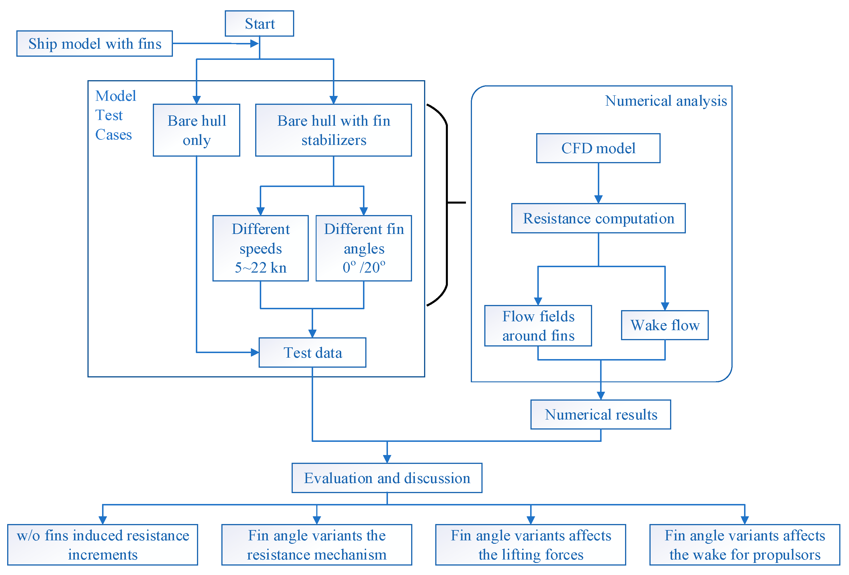
1.3. Methodology

The technical routes of the study are demonstrated as follows, shown in Figure 2. The model test was fulfilled at the Shanghai Jiao Tong University (SJTU) towing tank under various test conditions for different speeds, with/without fin stabilizers.

Then, the Reynolds Average Navier–Stokes (RANS) solver and Star-CCM+ were applied for numerical analysis. The numerical and experimental data were compared while the flow details were investigated.

2. Experiment Setup

2.1. Test Preparation

Firstly, an experimental analysis was conducted. A resistance series test was carried out at the multi-functional ship model towing tank at SJTU. The towing tank dimensions were equal to 300 m × 16 m × 7.5 m with a maximum carriage speed of 10 m/s. A medium-sized cruise ship model of around 50,000 GT was built, and the scale ratio was 1:55. The main parameters of the model ship are listed in

Table 1. Main parameters of the model.

Items	Symbols	Value
Length between perpendiculars	LPP/m	3.725
Breadth	B/m	0.564
Draft	T/m	0.1173
Displacement	Δ/t	0.1742
Wetted surface	Sw/m2	2.362
Center of gravity	LCG/m	1.611
Center of gravity	KG/m	0.287
Fin sectional hydrofoil		NACA0021
Fin chord length	m	0.06
Aspect ratio		2.05
Fin length	m	0.12376

.

Figure 3 shows the entire model with a pair of fin stabilizers installed at the middle of the ship about 45% Lpp to the stern boundary, both at port and starboard, 37% D above the baseline with 10° inclination, displayed in Figure 3a,b. The wing section of the fins is NACA series, and the working angle ranges are ±20°, avoiding the stall, as shown in Figure 3c. The geometry parameters of the fin are also listed in Table 1.

Various test cases were conducted to investigate the resistance due to the fins, as listed in

Table 2. Test cases.

No.	Vs (kn)	Fr	Vm (m/s)	W/O Condition
				Without	With Fin Angle
					0°	20°
1	5	0.057	0.3468	~	④	⑧
2	14	0.159	0.9711	①	⑤	⑨
3	18	0.204	1.2485	②	⑥	⑩
4	22	0.249	1.5260	③	⑦	⑪

. Eleven test series cases covered different fin angles and with/without fins at different ship speeds.

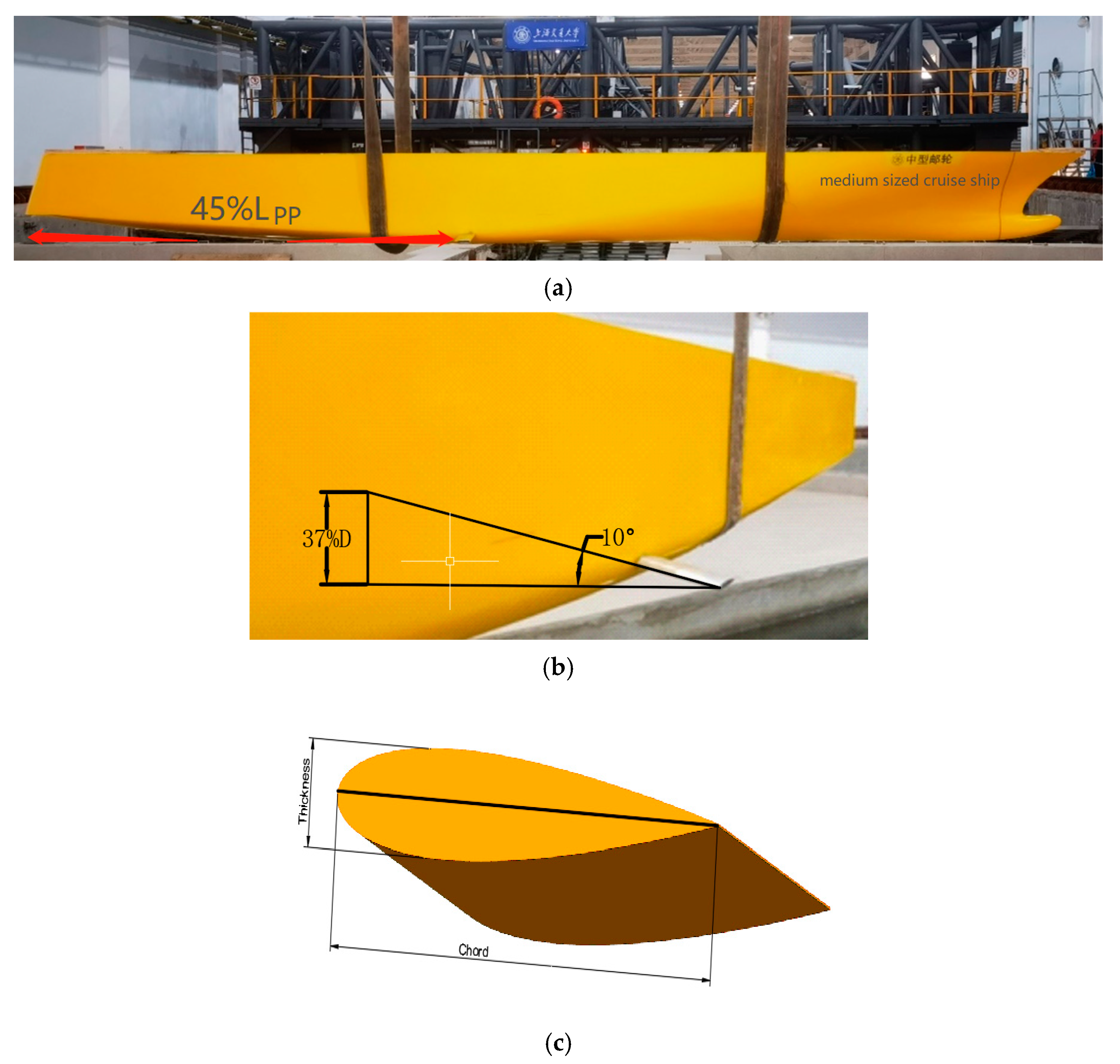
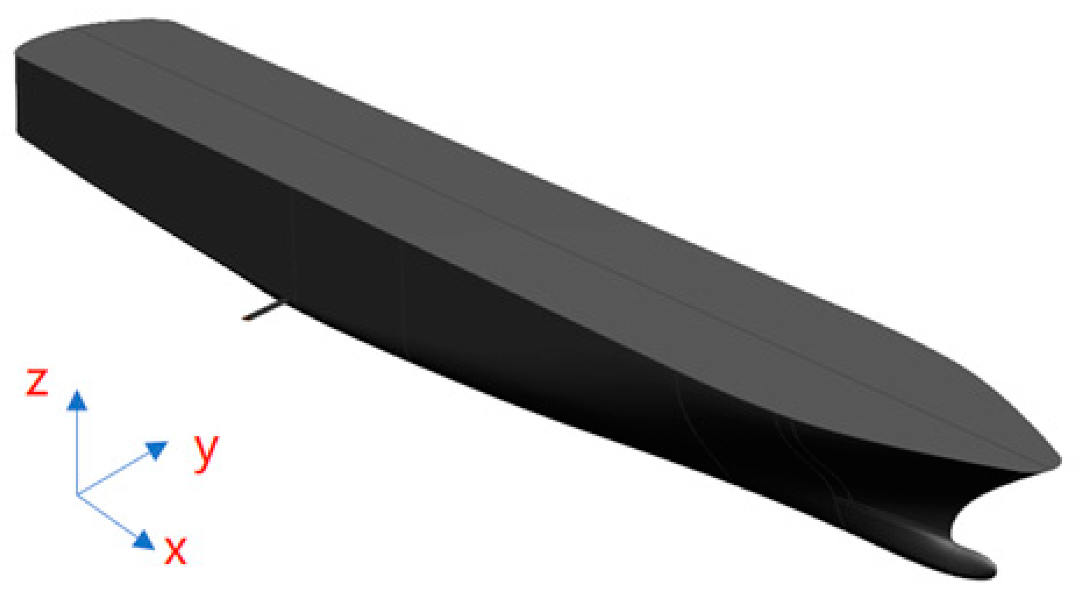
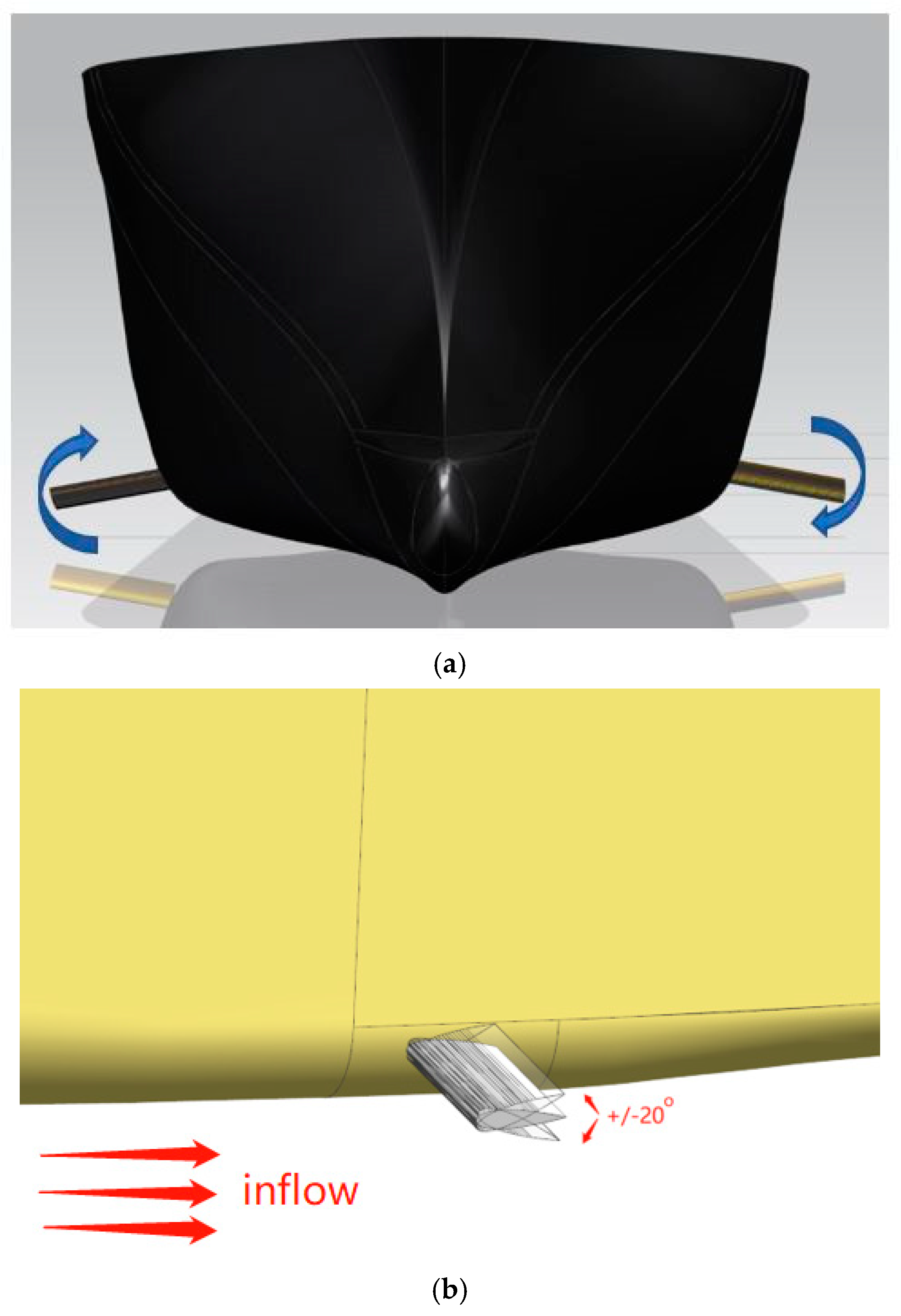
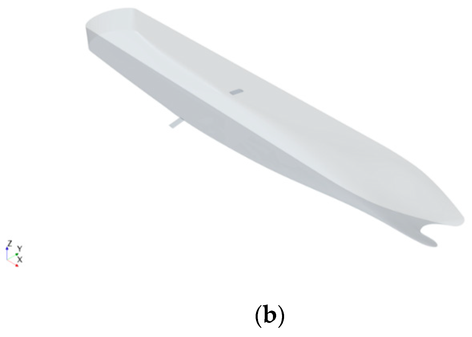
2.2. Geometry Model

The exact ship model with a pair of fins was built, as shown in Figure 4. The fins were mounted beneath the water line at the bilge. Different angles were achieved by rotating along the rotation axis.

It is worth mentioning that the fins at each side are not always rotated symmetrically. When the angle is at the maximum degree, asymmetric rotation happens, as shown in Figure 5. One fin is rotated clockwise, whereas the other is rotated counter-clockwise, aiming to achieve better anti-rolling lifting forces. The portside fin rotates upward while the starboard fin rotates downward.

3. The Numerical Analysis

The numerical methods were applied for hydrodynamic performance evaluation and flow details. In this section, a numerical analysis is conducted and compared to test the data. The detailed flow characteristics are analyzed to discover the fins’ hydrodynamic performance at low and moderate speeds.

3.1. Governing Equations

The RANSE method is used for the numerical simulation in model scale. The continuity and momentum conservation equations are as follows:

$$\frac{\partial {\overline{u}}_i}{\partial x_i}=0$$

(1)

$$\frac{\partial \left(\rho {\overline{u}}_i\right)}{\partial t}+\frac{\partial }{\partial x_j}\left(\rho {\overline{u}}_j{\overline{u}}_i\right)=-\frac{\partial \overline{p}}{\partial x_i}+F_i+\frac{\partial }{\partial x_j}\left({\sigma }_{ji}+R_{ji}\right)$$

(2)

where $R_{ji}=-\rho \overline{u_i^{\prime }{u}_j^{\prime }}$ is the Reynolds stress term or turbulence stress term; this new unknown variant after the average N-S equation leaves the equation unclosed. In order to close the equation, the SST K-Omega turbulence model must be added. According to the Boussinesq assumption, $R_{ji}=R_{ij}={\mu }_T{S}_{ij}-\frac{2}{3}\rho k{\delta }_{ij}$, where ${\mu }_T$ is the turbulent Eddy Viscosity coefficient. Given ${\mu }_T=\rho \frac{k}{\omega }$, the governing equations about turbulence kinematic k and dissipation rate $\omega$ are as follows:

$$\frac{\partial \rho k}{\partial t}+{\overline{u}}_j\frac{\partial \rho k}{\partial x_j}={\tau }_{ij}\frac{\partial {\overline{u}}_i}{\partial x_j}-\beta \times \rho k\omega +\frac{\partial }{\partial x_j}\left[\left(\mu +{\sigma }_k{\mu }_T\right)\frac{\partial k}{\partial x_j}\right]$$

(3)

$$\frac{\partial \rho \omega }{\partial t}+{\overline{u}}_j\frac{\partial \rho \omega }{\partial x_j}=\alpha \frac{\omega }{k}{\tau }_{ij}\frac{\partial u_i}{\partial x_j} -\beta \rho {\omega }^2+\frac{\partial }{\partial x_j}\left[\left(\mu +{\sigma }_{\omega }{\mu }_T\right)\frac{\partial \omega }{\partial x_j}\right]+2\rho \left(1-F_1\right){\sigma }_{\mathsf{\omega }2}\frac{1}{\omega }\frac{\partial k}{\partial x_j}\frac{\partial \omega }{\partial x_j}$$

(4)

where F₁ is the combined coefficient, equal to 1 close to the wall and 0 far from the wall, combining K-Omega and K-Epsilon models. Assisting equations and parameters can be found in the published literature [27].

3.2. Calculation Setup

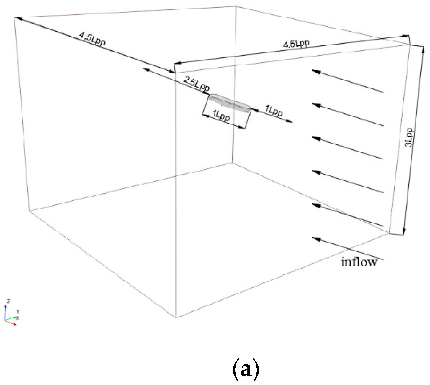
3.2.1. Computational Domain

The computational domain used in the resistance tests is a whole ship model with a pair of fins on each ship side, which considers the asymmetry cases. The hull motion was captured in the resistance test based on overset grid technology. The background domain was cubic with dimensions of 4.5 L_PP × 4.5 L_PP × 3 L_PP, as shown in Figure 6a. The boundary conditions of the inlet, bottom, and top of the background domain were set to the velocity inlet; the outlet was set to the pressure outlet, and the two sides were symmetrical planes, as shown in Figure 6b.

3.2.2. To Avoid Wave Reflection

In order to avoid the reflection of the truncated boundary wave on the free surface, a wave-absorbing damping area is introduced on the free surface related to the truncated boundary. By adding a damping term to the free surface boundary conditions:

$$\{\begin{array}{c}\frac{d\zeta }{dt}=\frac{\partial \varphi }{\partial z}-\frac{\partial \varphi }{\partial x}\frac{\partial \zeta }{\partial x}-\frac{\partial \varphi }{\partial y}\frac{\partial \zeta }{\partial y}-v\zeta \\ \frac{d\varphi }{dt}=-\left(\frac{1}{2}\nabla \varphi \cdot \nabla \varphi +g\zeta \right)+\frac{\partial \varphi }{\partial z}\left(\frac{\partial \varphi }{\partial z}-\frac{\partial \varphi }{\partial x}\frac{\partial \zeta }{\partial x}-\frac{\partial \varphi }{\partial y}\frac{\partial \zeta }{\partial y}\right)-v\varphi \end{array}\mathrm{on}z=\zeta \left(x,y,t\right)$$

where $v$ is a quadratic damping factor based on the generalized spatial variable $s$.

$$v\left(s\right)=\{\begin{array}{cc}0& \mathrm{for}s\le s_0\\ \mu \omega {\left(\frac{s-s_0}{\lambda }\right)}^2& \mathrm{for}s>s_0\end{array}$$

where $s_0$ marks the beginning of the wave-chopping damping region; $\mu$ is a tuning factor; and $\omega$ and $\lambda$ are the frequency and length of the damped wave, respectively. The extent of the damping region should be at least one wavelength.

3.2.3. Air and Water Interface

The air–water interaction is simulated based on the volume-of-fluid method (VOF method). The VOF model is an interface tracking method based on an Euler grid. The fluid volume function value on each control unit is determined by the fluid volume contained in the unit. In this way, the variables and properties in any control volume can be obtained according to the fluid volume function value, and the transport equation can be solved accordingly to capture the motion interface.

We define a scalar function $f$ such that $f=1$ when liquid is present in the control unit and $f=0$ when no liquid is present. The volume function $F$ is defined as the ratio of the fluid volume to the control unit volume, which is equal to the integral of the scalar function $f$ over the control volume divided by the control unit volume.

Since the volume of the control unit is constant, the fluid volume function satisfies the continuity equation:

$$\frac{\partial F}{\partial t}+\frac{\partial \left(u_{i}F\right)}{\partial x_i}=0$$

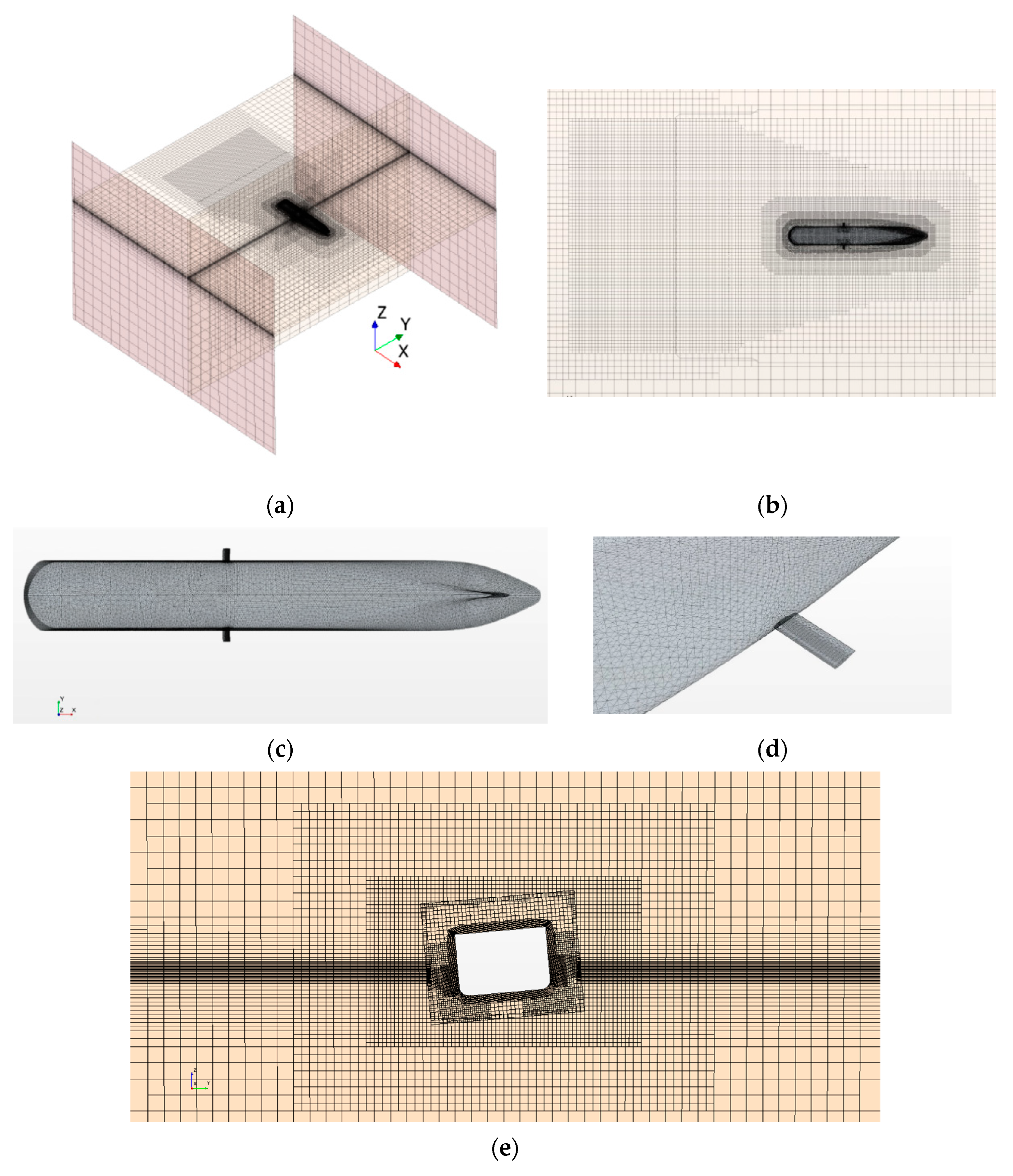
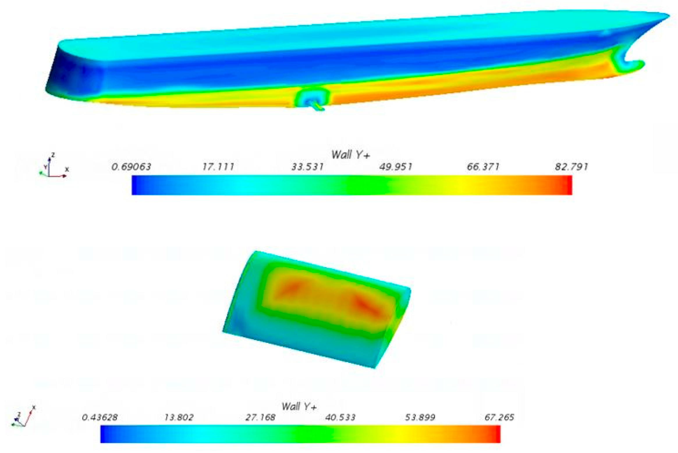
3.3. Mesh Generation

The mixed grids strategy was used to generate suitable grids (see Figure 7). Five sets of grids from G1 to G5 were investigated. Volume mesh comparisons are listed in

Table 3. Grid comparisons at 0° fins.

Items	Volume Meshes (Unit: M)	Rtm (N)	$\mathbf{error}=\left({\mathit{G}}_{\mathit{i}}-{\mathit{G}}_{\mathit{i}-1}\right)/{\mathit{G}}_{\mathit{i}-1}$
G1	1.02	8.4	−1.31%
G2	1.36	8.29	−0.72%
G3	1.80	8.23	−0.49%
G4	3.08	8.19	−0.12%
G5	7.02	8.18

. According to the results and accounting for the computational cost, G4 was adopted as the suitable main grid for further calculations.

To establish the wall function, the dimensionless numbers u⁺ and y⁺ are introduced to describe the velocity and distance, respectively:

$$\begin{array}{c}{u}^{+}=\frac{u}{u_e}\\ y^{+}=\frac{\mathsf{\Delta }y\rho u_{\tau }}{\mu }=\frac{\mathsf{\Delta }y}{v}\sqrt{\frac{{\tau }_w}{\rho }}\end{array}$$

where u is the average fluid velocity; u_τ is the wall friction velocity, $u_{\tau }=\sqrt{{\tau }_w/\rho }$; ${\tau }_w$ is the wall shear stress; and $∆y$ is the distance from a point to the wall. The boundary layer number at the fin area is set to 6 and the thickness is 0.015 m, with a growing ratio of 1.2, ensuring the y⁺ along with the computational domain is controlled below 90 and especially within 68 around the fin area.

The distribution is shown in Figure 8.

4. Results and Discussions

Based on the experimental studies and numerical computations, the fin stabilizers’ increased resistance was compared in this section at different ship velocities with two typical angles.

4.1. Experimental Results

The experimental test results are shown in Figure 9. With an increased fin angle, at a low Froude number, the differences between the fin angles are more significant than expected as an appendage, from 11.70 to 21.97% with increasing speeds. Since the fin stabilizer is not effective at low speeds of about 5 kn, only moderate speed tests were conducted for without-fin conditions.

According to

Table 4. The resistance increment ratio of model tests with fins at different speeds (o = without).

No.	Fr	${\mathsf{\epsilon }}_1=\left(0°-\mathbf{o}\right)/0°$	${\mathsf{\epsilon }}_2=\left(20°-0°\right)/20°$
1	0.057	~	11.70%
2	0.159	11.25%	20.96%
3	0.204	7.33%	21.97%
4	0.249	6.18%	21.38%
Average		8.25%	19%

, the average resistance without fin stabilizers was 8.252% smaller than 0° fins. The latter was 19% smaller than the asymmetrical 20°. The resistance was highest at Fr = 0.204, with nearly 22% extra drag. For 0° fins, such as ${\mathsf{\epsilon }}_1$, the increments of the resistance compared to the bare hull decreased with rising speeds because the frictional resistance component was maintained by a continuously wet surface, whereas the hydrodynamic component increased.

The test for each case has been carried out according to the ITTC model test procedure, Uncertainty Analysis in EFD, Uncertainty Assessment Methodology’ in QM 7.5-02-01-01. The value of the form factor k is 0.126, with an expanded uncertainty of ±0.0087132 (±6.9%).

Furthermore, the resistance forces and free surface variations were recorded by instruments for further analysis.

4.2. Verifications for EFD and CFD

The experimental and numerical results are shown in Figure 10, which compares experiment results without fins and with 0° and 20° fin angles. The fin induces the resistance increment in the frictional and hydrodynamic parts so that the increment portion is not as small as 2% [28]. The fin-induced resistance should be carefully considered. The CFD results were also in good accord with the test data, with the maximum error margin within 4.87%.

Due to the raised fin angle by the CFD and EFD, the resistance increment predictions, agreed well within 3%, as shown in

Table 5. Resistance when fins are at two angles.

No.	Fr	(0°–20°)/20°		Error (%)
		Rtm_EFD (%)	Rtm_CFD (%)	EFD—FD
1	0.057	−11.70%	−14.65%	2.94%
2	0.159	−20.96%	−22.84%	1.88%
3	0.204	−21.97%	−21.84%	−0.13%
4	0.249	−21.38%	−20.27%	−1.11%

. The CFD calculation results in Figure 10 are slightly larger than the test results of total resistance. With the smallest absolute resistance value, the ratio was higher than the others at low speed.

In general, the CFD and EFD results were in agreement.

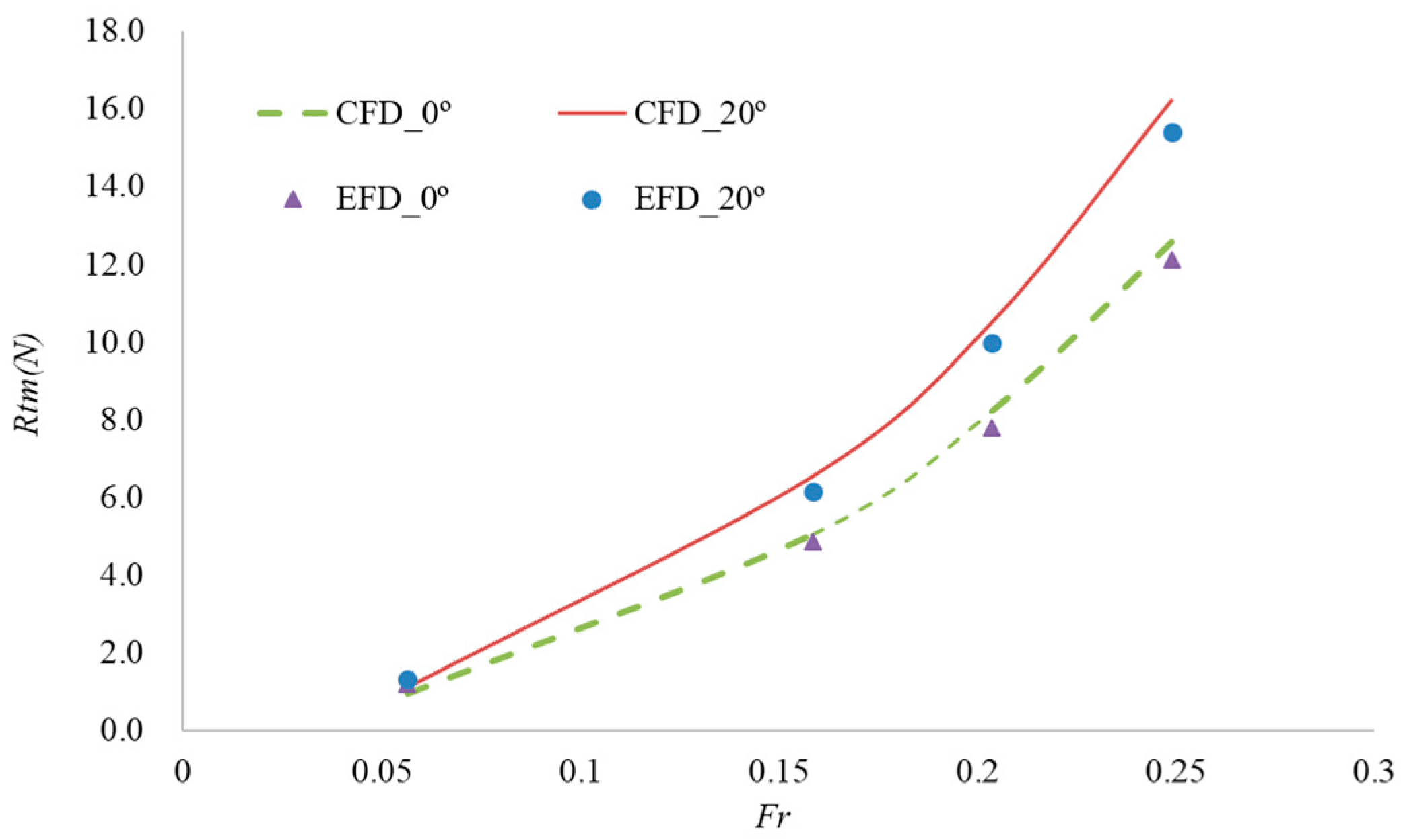
4.2.1. W/O Fin Comparisons

The flow characteristics at service speed were investigated. The pressure coefficients and skin friction coefficients of the hull and free surface are shown in Figure 11. The existing fins increased the friction at the corresponding aft part of the hull because the corresponding pressure increased. Another feature of the pressure distribution is that the high-pressure area at the bottom is reduced and separated into two parts. Asymmetric 20° fins lead to asymmetrical pressure distribution at the bottom.

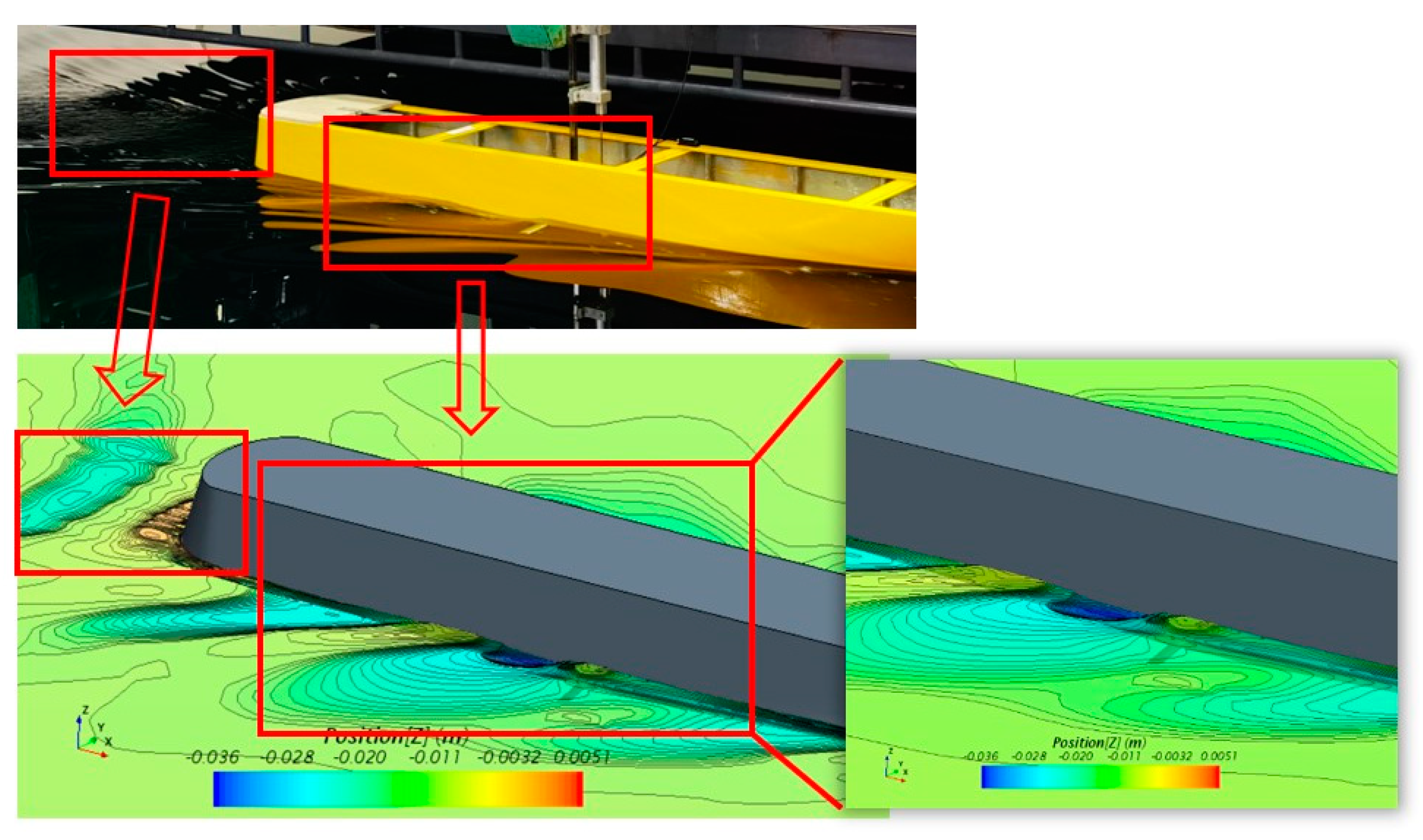
4.2.2. Free Surface Comparisons

Figure 12 shows the fin-area-induced wave elevation, which can be clearly observed with a larger amplitude of ship waves. In general, fin-induced extra waves at the ship’s middle correspondingly increase the stern wake amplitude.

The free surface of the model test and numerical calculation results were compared and are shown in Figure 13. The ship wave was slightly disturbed around the fin area, which was captured by the numerical method with the crest and trough leeward of the fin. The slipstream off the stern was also simulated in detail.

4.2.3. With 20° Fins—Asymmetry Condition

The maximum angle of the fin rotation is 20° due to stall limitations. Similarly, Figure 14 shows the ship waves captured by the CFD method, especially around the fin area with the leeward trough and crest illustrated. The slipstream behind the ship was also simulated in good accordance.

The asymmetry fins were analyzed, leading to a different flow at the port and starboard. Figure 15 demonstrates the velocity increments around the fin areas, without fins, at a 0° angle, and at a 20° angle.

At a maximum fin angle of 20°, the fins at each side turn in the opposite direction to derive higher damping. It is worth investigating the flow details of this situation. The velocity specified for the fins on both sides with free surface elevations is shown in Figure 16a, which demonstrates a free surface at the same height, while the portside is lower than that of the starboard, though both sides are elevated. The existing fins increase the free surfaces vertically above, but in a different way because of the different rotation direction. Figure 16b provides an axial velocity distribution at the sectional surface of the fin with streamlines in order to display the flow around the fins.

4.3. Fin Drag Evaluation

At the specified Reynolds number Re, $\rho$ is the fluid density, $U_f$ is the free-steam velocity, and A is the fin area; $F_L$ and $F_D$ represent the lifting and drag forces induced by fin foil at a certain attack angle, respectively. Then, ${\mathrm{C}}_L$ and ${\mathrm{C}}_D$ can be defined as follows Equations (5) and (6):

$${\mathrm{C}}_L=\frac{F_L}{0.5\rho A{U}_f^2}$$

(5)

$${\mathrm{C}}_D=\frac{F_D}{0.5\rho A{U}_f^2}$$

(6)

Due to unsteady local velocities, a steady evaluation method of average Re is introduced, where $\mu$ is the coefficient of dynamic viscosity and L is the fin length.

$$Re=\frac{\rho U_{f}L}{\mu }$$

(7)

According to the local Reynolds number of fins, the fin drags were computed and compared with EFD results, and the drag of two fins is listed in

Table 6. Fin drag analysis at 20° in model scale (unit: N).

Fr	Re	Fin Drags by EFD (a)	Fin Drags by CFD (b)	Steady Estimation (c)
0.159	1.19 × 105	1.834	1.749	2.598
0.204	1.53 × 105	2.7596	2.7617	3.946
0.249	1.87 × 105	4.0437	4.0648	6.098

.

For detailed analysis of fin effect, the comparisons with local pressure and friction at the fin surface at various ship speeds were computed, shown in Figure 17. At high speeds, the limited coefficient range for comparison made empty areas beyond the limitation. For friction development at fin areas, with increasing speeds, there are two concentrated zones with a higher zone near the hull at the 0° fin. However, at the 20° fin, the concentration happened at the leading edge. For pressure, the high pressure center enlarged to the leading edge with a larger fin angle, which mainly provides lifting forces.

The error analysis is listed in

Table 7. Error analysis in model scale (unit: %).

Fr	${\mathsf{\epsilon }}_{3 }=\left(\mathbf{w}-\mathbf{o}\right)/\mathbf{o}$	${\mathsf{\epsilon }}_4=\left(\mathbf{b}-\mathbf{a}\right)/\mathbf{a}$	${\mathsf{\epsilon }}_5=\left(\mathbf{c}-\mathbf{b}\right)/\mathbf{b}$
0.159	183.40	−4.63	48.54
0.204	275.96	0.08	42.88
0.249	404.37	0.52	50.02

, where a, b, and c represent the three methods listed in Table 6.

From the above tables, the fin drags derived by EFD can reach four times at the 20° fin angle, the significance of which cannot be neglected. The drags increased with rising speeds.

The CFD method predicted the drag of fins at a larger angle, but the steady method was overestimated by about 50% when adopting the average velocity and neglecting hull–fin interaction.

4.4. Propulsor Inflow Analysis

Another fin stabilizer effect is that it changes the wake, especially disturbing the inflow for the propulsors. The distribution of nondimensional wake fraction, V_axial/V_ship, at the propulsor disks is shown in Figure 18, with the different fin angles and bare hull without fins.

Moreover, the circumferential velocity comparisons were made, shown in Figure 19. There are two bilge vortices that can only be observed without fins and with 20° fins, but the strength distributions are different at the bottom flow fields. The velocity distribution of 0° fins is different from the others, with the smaller bottom velocities, which should be noticed for propulsor design.

The propulsor hydrodynamic performance should be reconsidered with fins at various angles. From Figure 18, for propulsor inflow, the axial velocity distribution is nearly the same, neglecting the coupling effect. From Figure 19, the circumferential velocities differ significantly.

4.5. Fin Effect in Waves

The overset technique was employed for the computation with the grids shown in Figure 7, in order to capture the motions induced by waves. In simulation, the fifth-order Stokes wave model is used [29]. This wave more closely resembles a real wave than a wave that is generated by the first-order method. The head wave profile and the wave phase velocity depend on the water depth, wave height, and current. The wave height is 0.03723 m, wave period is 0.845 s and wave length is 2.834 m.

In waves, the fin-induced resistance was computed and the results are shown in

Table 8. Fin drag analysis at 20° in model scale (unit: N). Fr = 0.204.

Condition	Drag in Calm Water (N)	Drag in Waves (N)	${\mathsf{\epsilon }}_6=\left(\mathbf{waves}-\mathbf{calm}\right)/\mathbf{waves}$
Without	7.42	7.672	3.29%
0° fin	7.926	8.020	1.17%
20° fin	10.11	10.244	1.31%

. The added resistance of the hull with fins increases less than that without fins.

Furthermore, the roll and pitch motion were calculated for the W/O fin condition with headsea conditions, shown in Figure 20. The uncontrolled fin is beneficial for reducing the ship motion; the reduction for roll is up to 52.6%, while that of pitch is 88% at 22 kn.

5. Conclusions

Fin stabilizer technology can effectively maintain the stability of cruise ships in complex sea conditions, provide guaranteed security on cruise voyages, and provide a high-quality travel experience for tourists.

In this paper, a medium-sized cruise ship W/O a fin stabilizer was investigated through experiments and numerical computations. Based on experimental data and simulation results, the following conclusions were drawn:

(1)

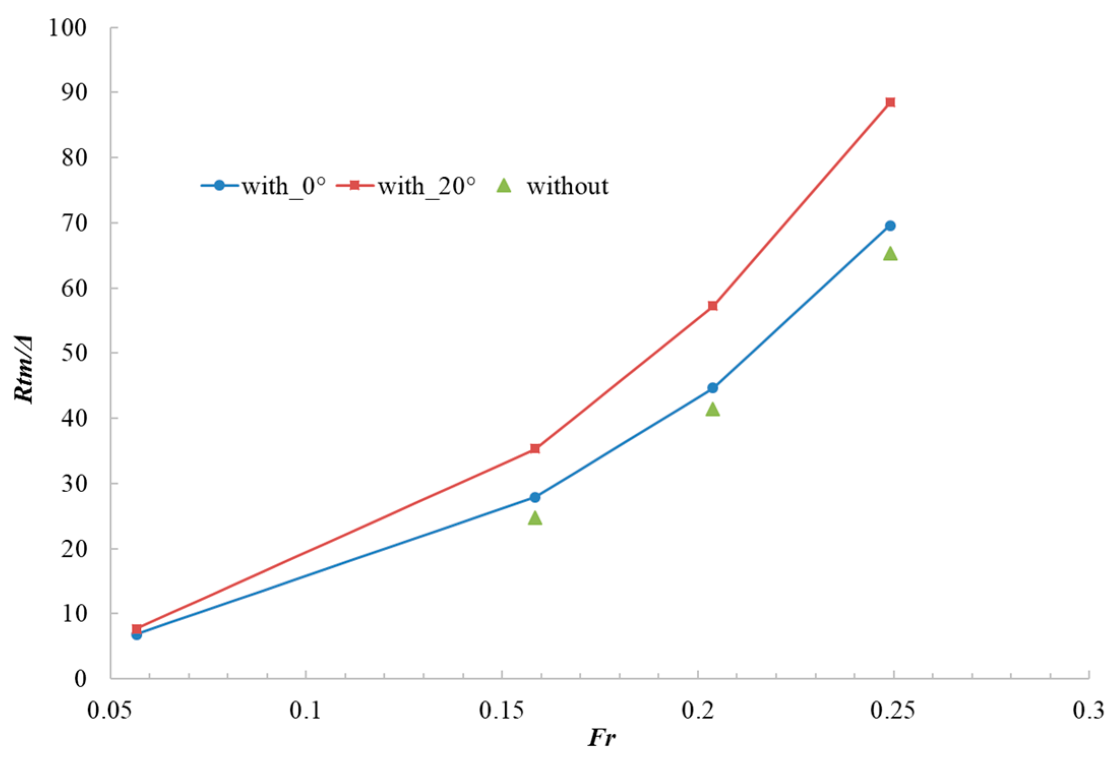
The EFD provided reliable qualitative resistances, with various overhang fins at different angles at various ship speeds. The average resistance increment was 8.252%, whereas it increased by up to 19% at the largest fin angle. The test data proposed a new understanding of the fin-induced resistance.

(2)

CFD analysis details the fins’ resistance characteristics at various ship speeds and fin angles. The numerical methods that predicted the resistance increments agreed with EFD, with an average error margin within 5%.

(3)

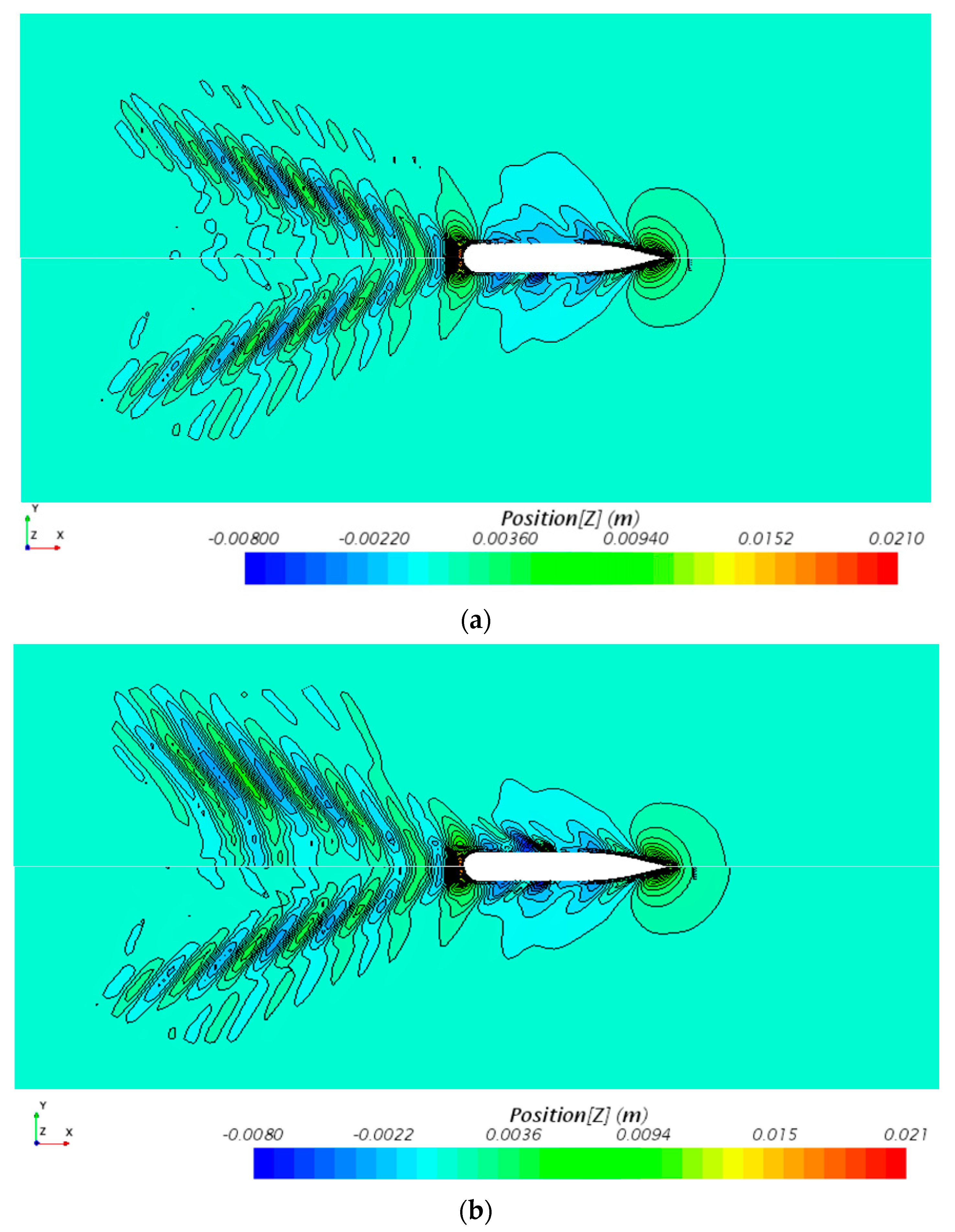
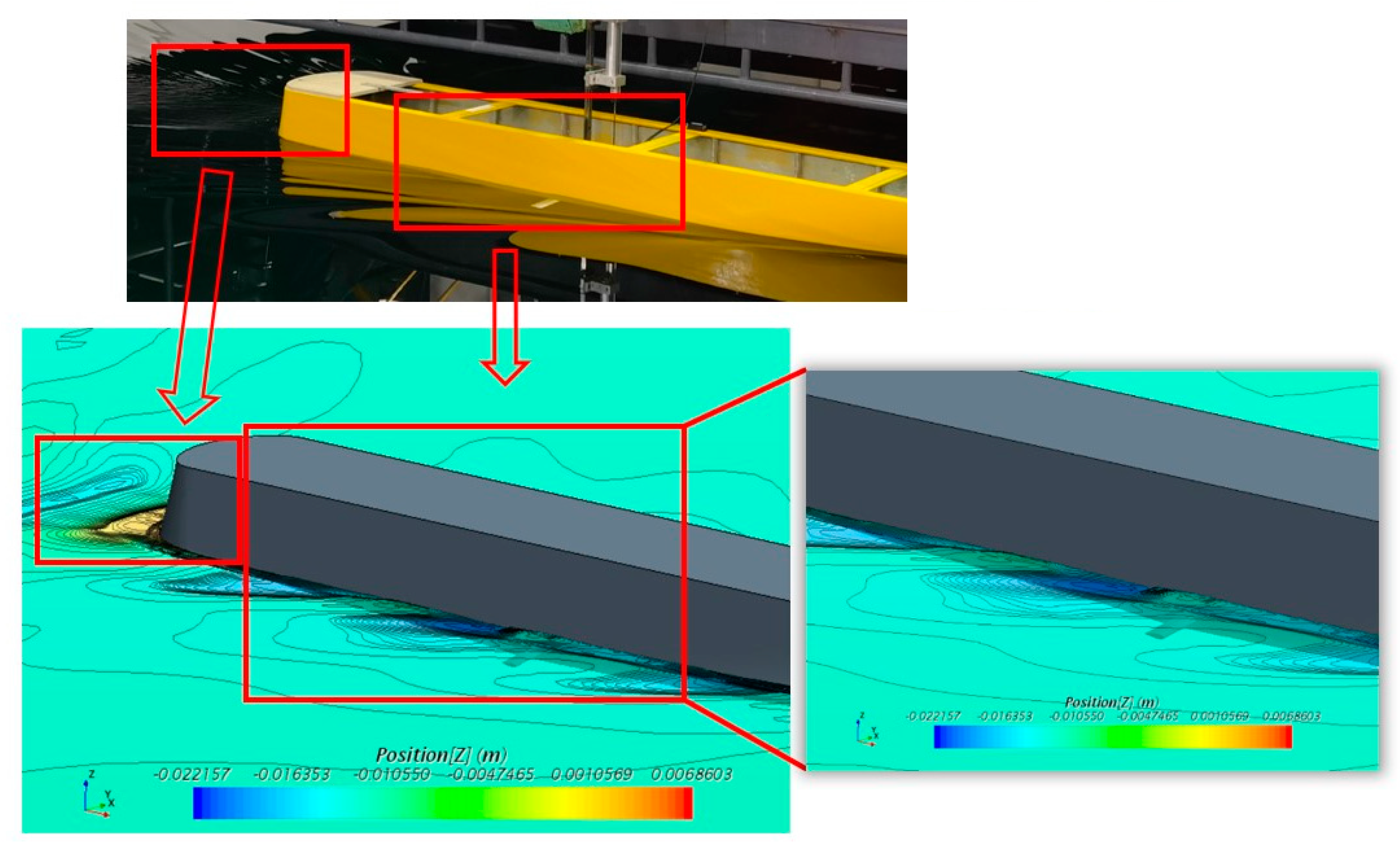
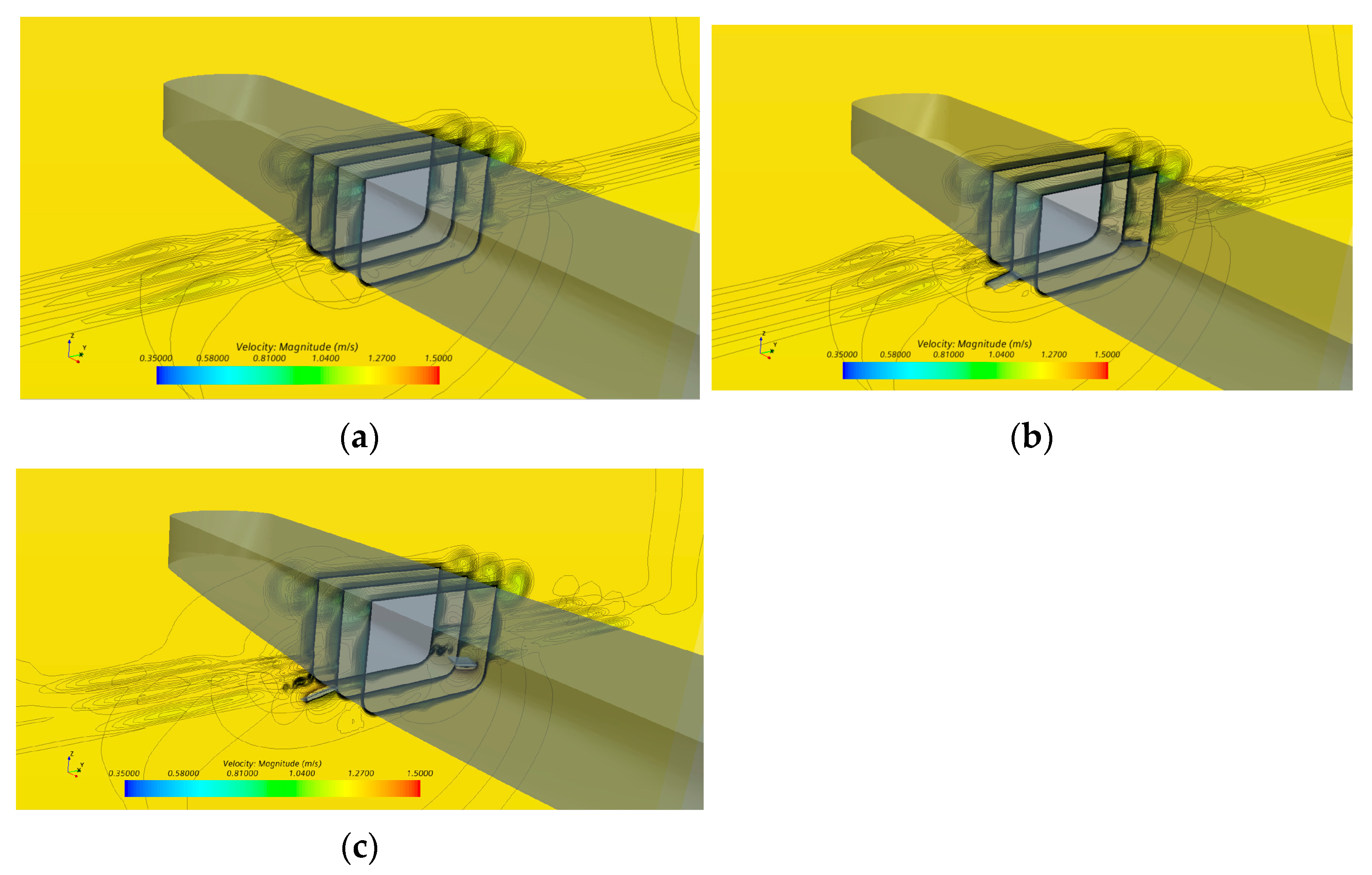
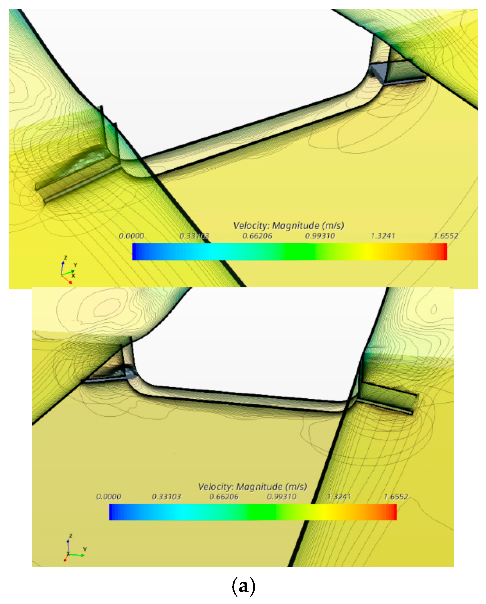
The CFD computation captured the ship wave in good accord with the EFD, especially ship waves near the fin area with the same crest and trough. The flow characteristics of the maximum fin angle of 20° was investigated, and the two sides with different velocity distributions were compared with EFD results.

(4)

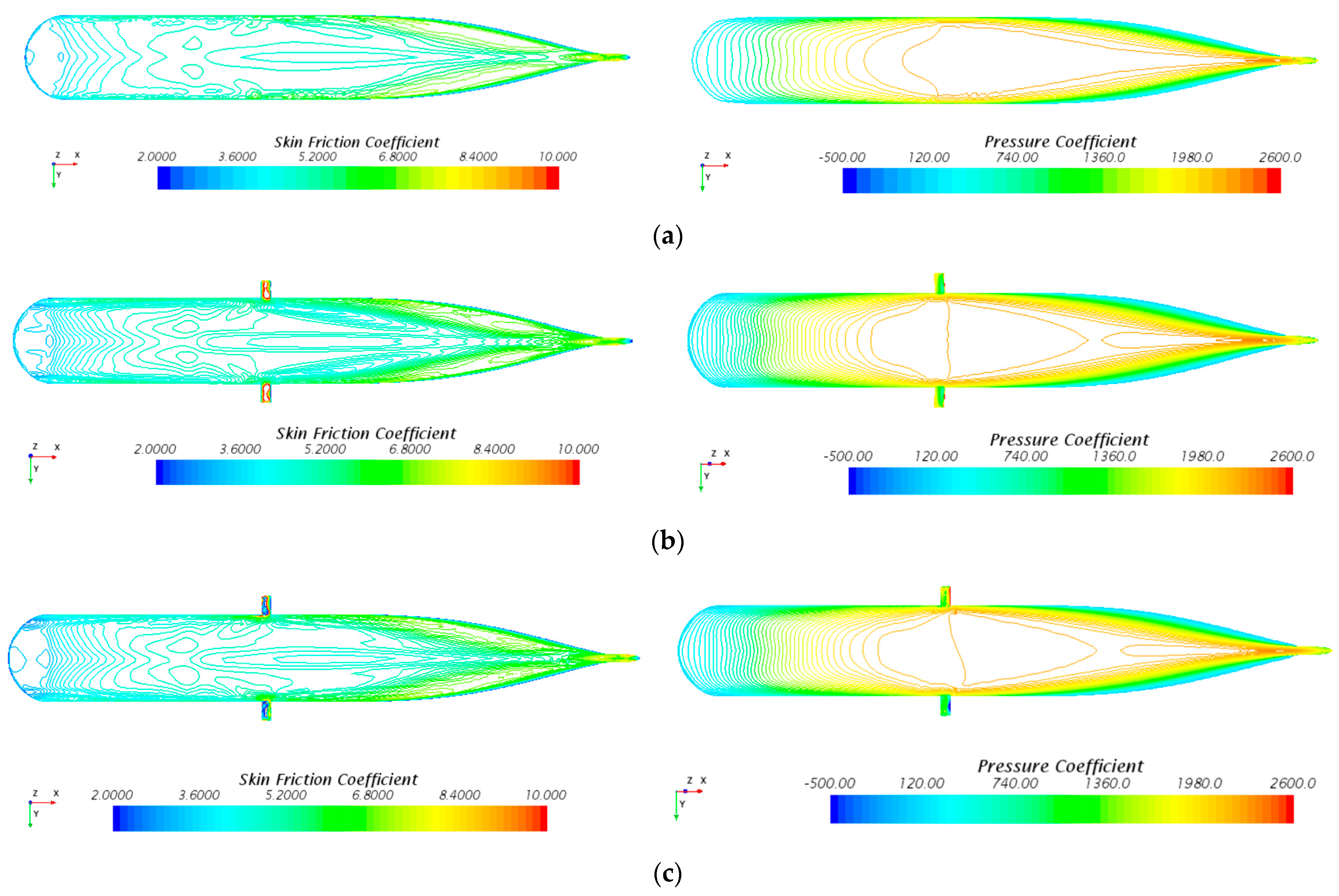
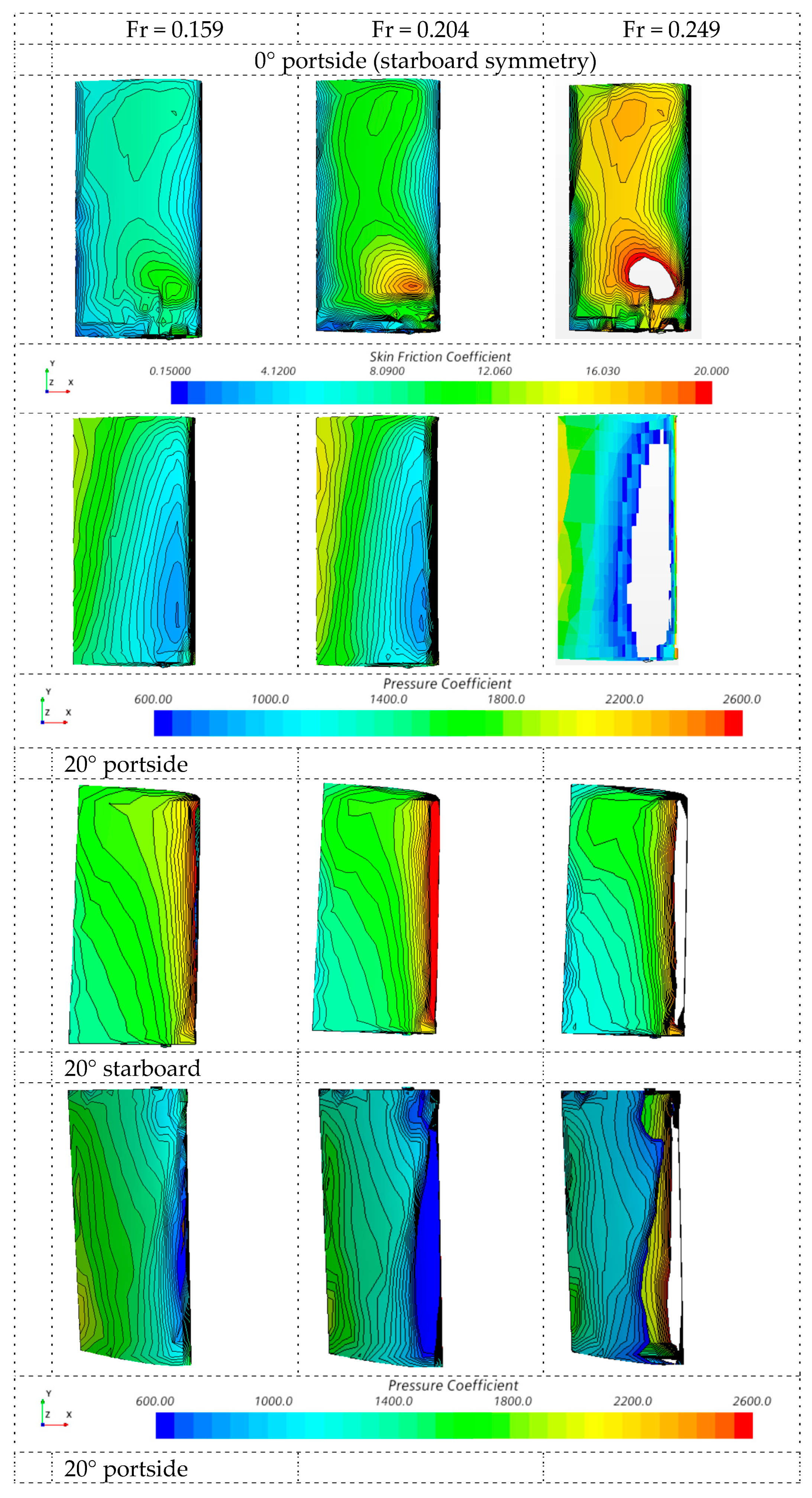
The fin drags derived by EFD can reach four times at the 20° fin angle, the significance of which cannot be neglected. The CFD, as an unsteady and steady method, was employed for fin drags, compared with the EFD. The CFD provided high-fidelity results, whereas the steady method overestimated by about 50%. From detailed computation, the high-pressure area moved to the leading edge with higher speeds, while the frictional area moved to the trailing edge.

(5)

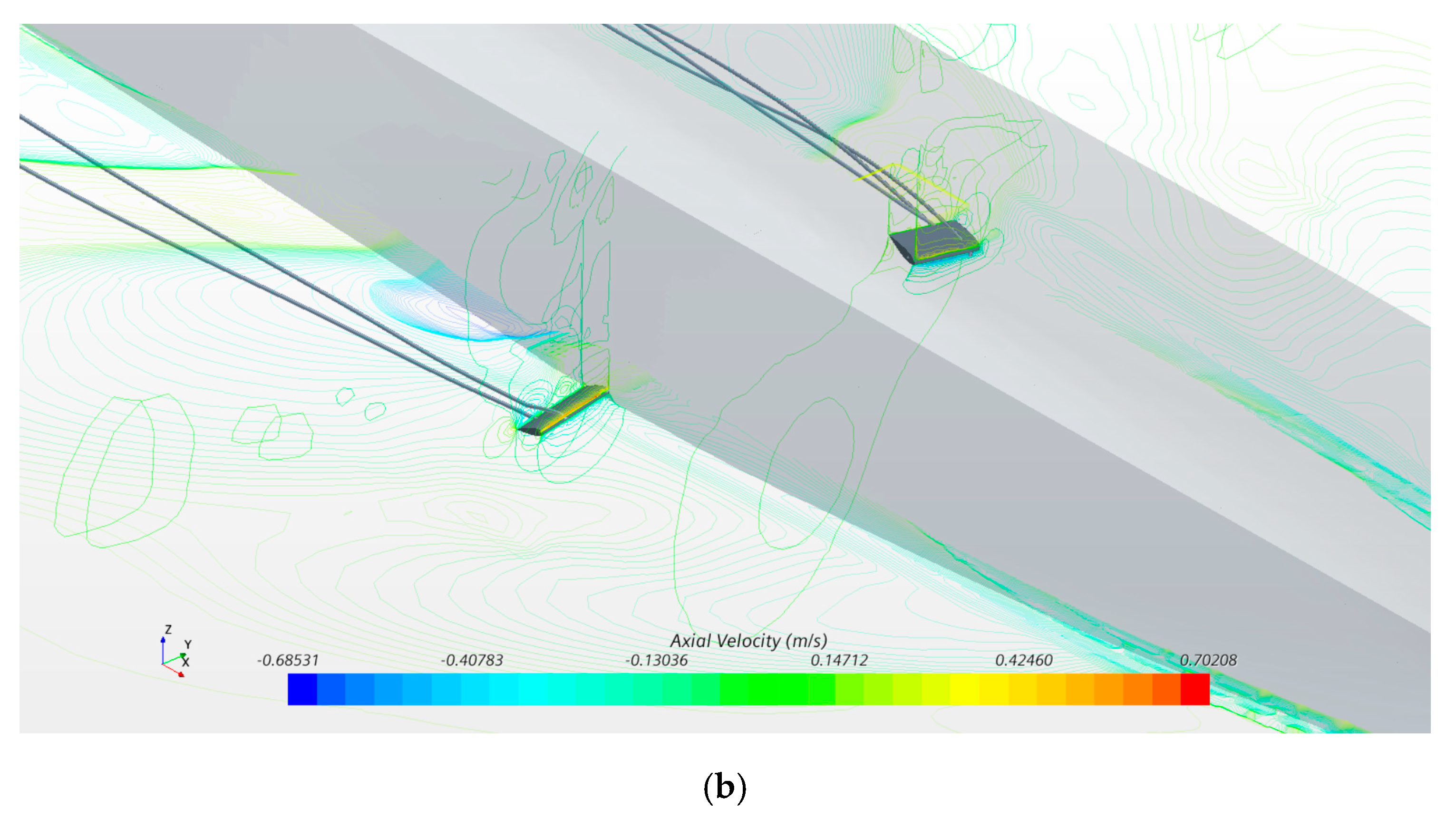
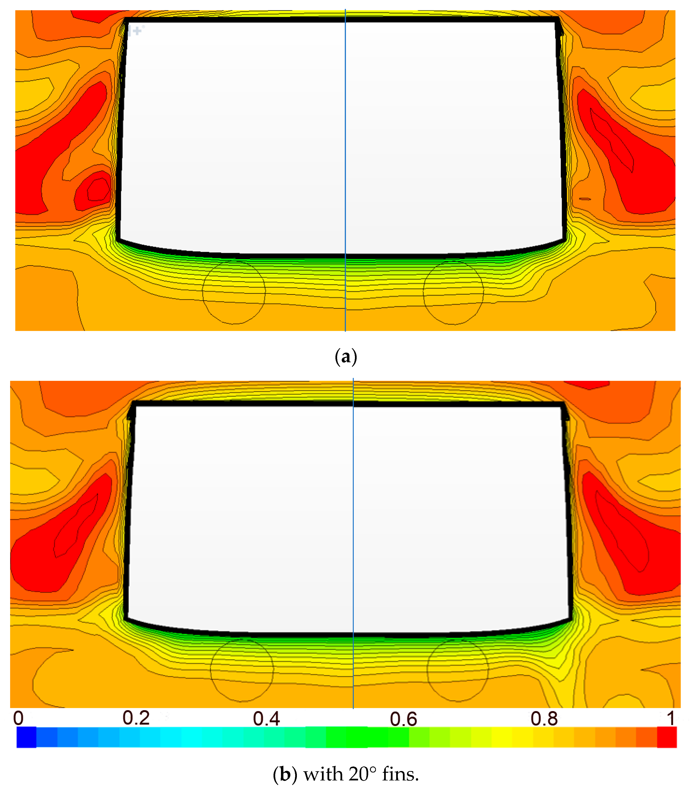
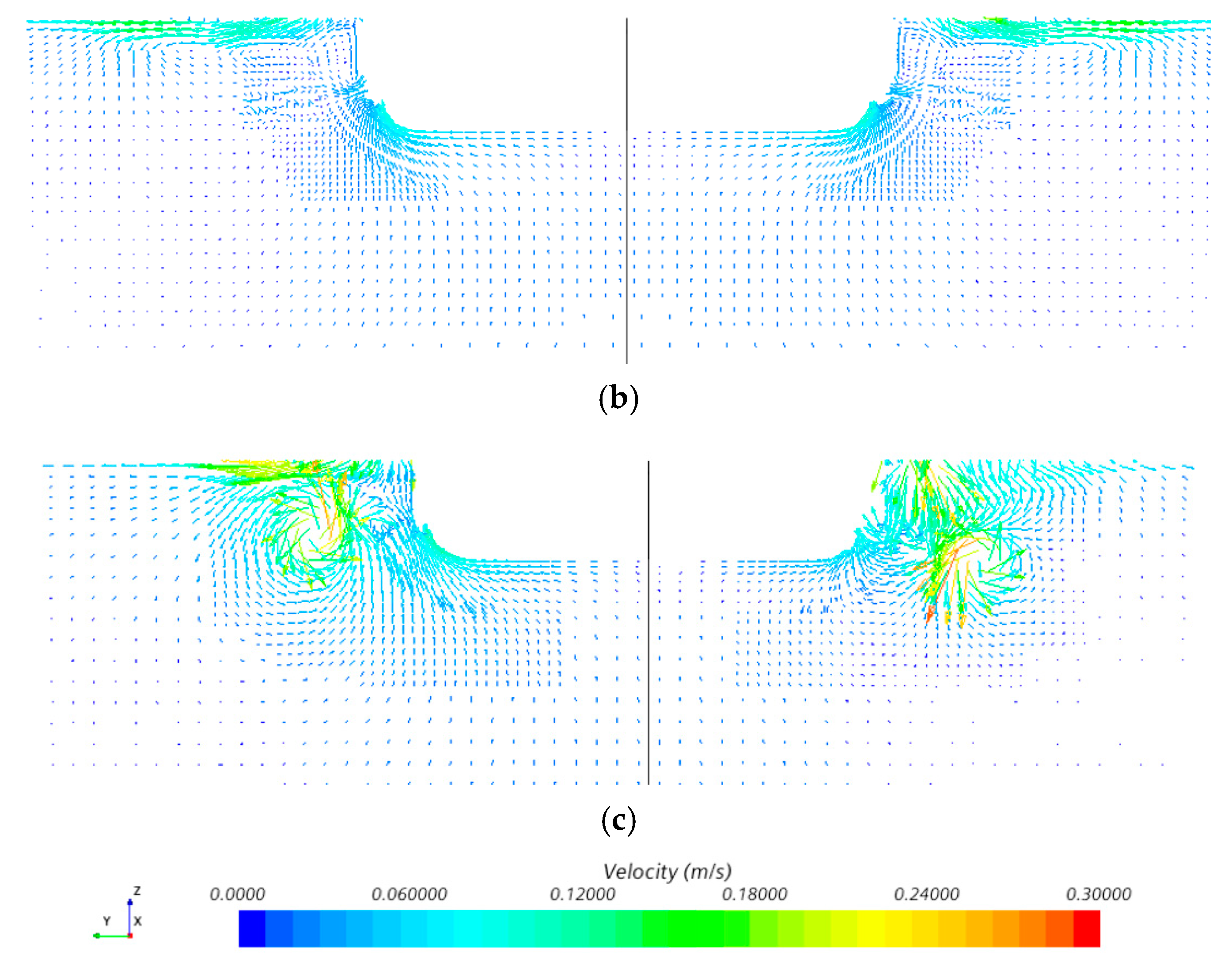
The velocity distribution at the propulsor disk was calculated and compared. The fin-induced inflow change cannot be ignored, especially circumferential velocities at different fin angles.

(6)

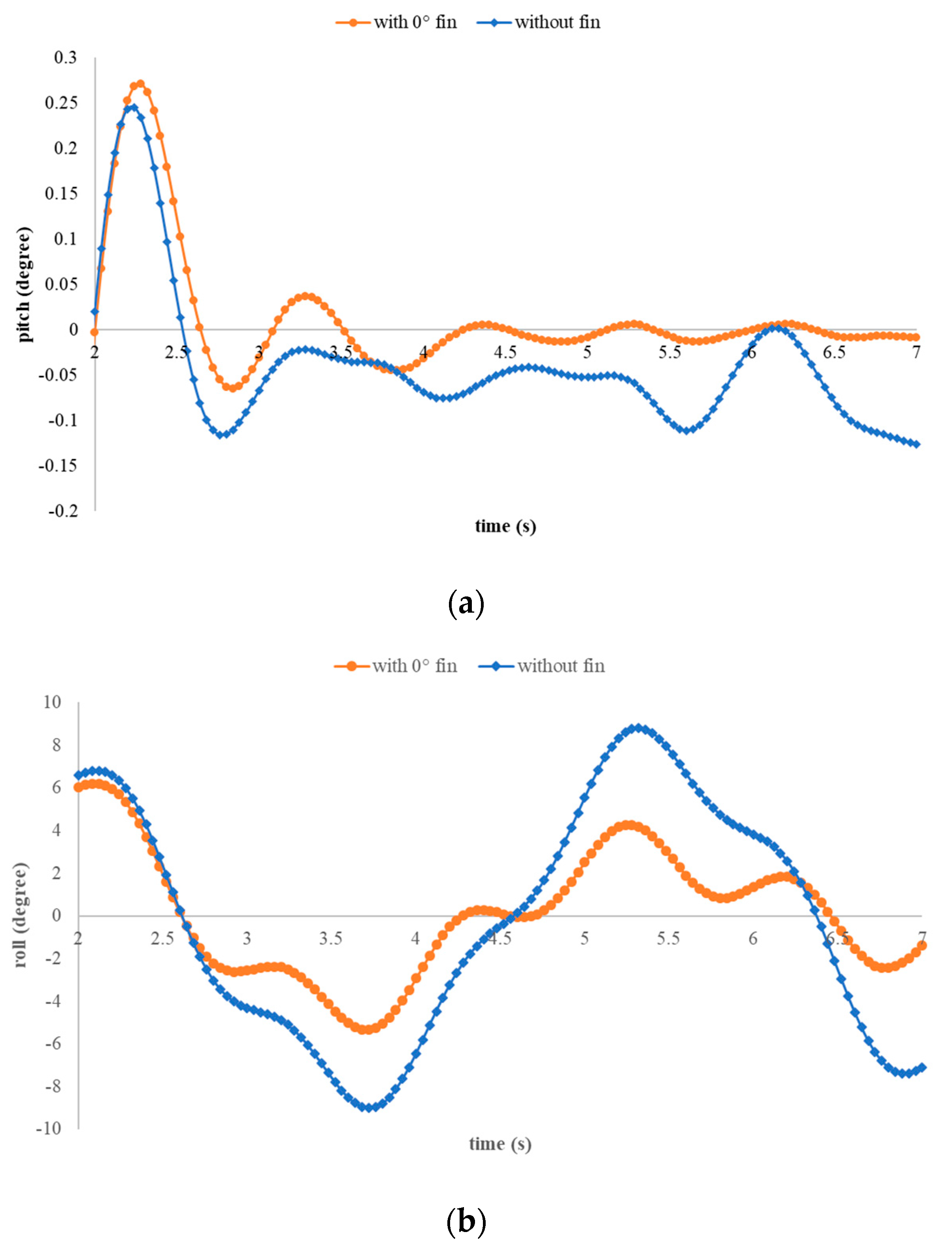
The fin effect in waves has been investigated. The added resistance of the hull with fins increases less than that without fins. The roll reduction by the uncontrolled fins is up to 52.6%, while that of pitch is 88% at 22 kn.

This paper proposed a resistance analysis series for various fin angles and ship speeds beneficial to understanding net fin drag and proposing high-fidelity numerical analysis. The influences of the controlled fin stabilizers to the motions and interferences with the propulsors will be discussed in the future.

References

- Holden, C.; Perez, T.; Fossen, T. A Lagrangian approach to nonlinear modeling of anti-roll tanks. Ocean Eng. 2011, 38, 341–359. [Google Scholar] [CrossRef]
- Dreyfusi, E.D.; Brunsell, P.A. Moving Weight Ship Stabilizer. U.S. Patent 3,557,735A, 26 January 1971. [Google Scholar]
- Townsend, N.C.; Murphy, A.J.; Shenoi, R.A. A new active gyrostabiliser system for ride control of marine vehicles. Ocean Eng. 2007, 34, 1607–1617. [Google Scholar] [CrossRef]
- Surendran, S.; Kiran, V. Technical note Studies on the feasibilities of control of ship roll using fins. Ships Offshore Struct. 2006, 1, 357–365. [Google Scholar] [CrossRef]
- Liu, W.; Demirel, Y.K.; Djatmiko, E.B.; Nugroho, S.; Tezdogan, T.; Kurt, R.E.; Supomo, H.; Baihaqi, I.; Yuan, Z.; Incecik, A. Bilge keel design for the traditional fishing boats of Indonesia’s East Java. Int. J. Nav. Archit. Ocean. Eng. 2019, 11, 380–395. [Google Scholar] [CrossRef]
- Liang, L.; Zhao, P.; Zhang, S.; Yuan, J.; Wen, Y. Simulation and analysis of magnus rotating roll stabilizer at low speed. Ocean Eng. 2017, 142, 491–500. [Google Scholar] [CrossRef]
- Kongsberg Maritime. Available online: https://www.kongsberg.com/maritime/products/positioning-and-manoeuvring/fin-stabilisers (accessed on 22 June 2022).
- Sellars, F.H.; Martin, J.P. Selection and evaluation of ship roll stabilization systems. Mar. Technol. 1992, 29, 84–101. [Google Scholar] [CrossRef]
- Gaillarde, G. Dynamic Behavior and Operation Limits of Stabilizer Fins; International Maritime Association of the Mediterranean (IMAM): Creta, Greece, 2002. [Google Scholar]
- Gaillarde, G. Dynamic stall and cavitation of stabiliser fins and their influence on the ship behavior. In Proceedings of the 7th International Conference on Fast Sea Transportation (FAST), Ischia, Italy, 7–10 October 2003. [Google Scholar]
- Perez, T.; Blanke, M. Ship roll damping control. Annu. Rev. Control 2012, 36, 129–147. [Google Scholar] [CrossRef] [Green Version]
- Della Rosa, S.; Maceri, S.; Viola, I.M.; Bartesaghi, S. Design and optimization of a fin stabilizer using CFD codes and optimization algorithms. In Proceedings of the 16th International Conference of Ship and Shipping Research, Messina, Italy, 26–27 November 2009. [Google Scholar]
- Ram, B.R.R.; Surendran, S.; Lee, S.K. Computer and experimental simulations on the fin effect on ship resistance. Ships Offshore Struct. 2015, 10, 122–131. [Google Scholar] [CrossRef]
- Giallanza, A.; Elms, T. Interactive roll stabilization comparative analysis for large yacht: Gyroscope versus active fins. Int. J. Interact. Des. Manuf. 2020, 14, 143–151. [Google Scholar] [CrossRef]
- Kusdiana, W.; Semin; Ariana, I.M.; Kusuma, C.; Ali, B. Location Analysis of Patrol Boat Fin Stabilizer Based on Numerical Method. IOP Conf. Ser. Earth Environ. Sci. 2022, 972, 12002. [Google Scholar] [CrossRef]
- Jin, H.Z.; Zhang, X.F.; Luo, Y.M.; Li, D.S. Research on lift model of zero speed fin stabilizer. Ocean. Eng. 2007, 25, 83–87. [Google Scholar]
- Dallinga, R.P.; Rapuc, S. Merits of Flapping Roll Stabilizer Fins. In Proceedings of the HISWA Amsterdam Boat Show, Amsterdam, The Netherlands, 2–7 September 2014. [Google Scholar]
- Jin, H.Z.; Pan, Y.; Yang, B. Theoretical analysis of humpback whale fin stabilizer at a small angle of attack. J. Ship Mech. 2010, 14, 1219–1226. [Google Scholar]
- Song, J.; Jin, H.; Meng, L. Optimum Design of Aerofoil for Fin Stabilizer at Whole Speed Range. Shipbuild. China 2013, 54, 1–10. [Google Scholar]
- Koop, M.T. Method for Actively Damping a Ship’s Motion as Well as Such an Active Roll Stabilization System. U.S. Patent 9,527,557 B2, 27 December 2016. [Google Scholar]
- Liang, L.; Jiang, Y.L.; Zhang, Q.; Le, Z.W. Aspect ratio effects on hydrodynamic characteristics of Magnus stabilizers. Ocean Eng. 2020, 216, 107699. [Google Scholar] [CrossRef]
- Ye, X.; Wang, X.; Wang, Y.; Luo, Y.; Yang, G.; Sun, R. Design Features and Construction Enlightenments of Oasis-Class Luxury Cruise Ships. In Report on the Development of Cruise Industry in China; Wang, H., Ed.; Springer: Singapore, 2018. [Google Scholar] [CrossRef]
- Zhu, W. Study on stabilization system for large ships. Chin. Water Transp. 2012, 12, 69–70. [Google Scholar]
- Düz, B. Sensitivity Analysis in Parametric Rolling of a Modern Cruise Ship Using Numerical Simulations in 6-DOF. In Proceedings of the 39th International Conference on Ocean, Offshore and Arctic Engineering, Online, 28 June–3 July 2020. [Google Scholar]
- Kim, J.H.; Kim, Y.H. Motion control of a cruise ship by using active stabilizing fins. Proc. Inst. Mech. Eng. Part M J. Eng. Marit. Environ. 2011, 225, 311–324. [Google Scholar] [CrossRef]
- Lee, S.; Rhee, K.P.; Choi, J.W. Design of the roll stabilization controller, using fin stabilizers and pod propellers. Appl. Ocean. Res. 2011, 33, 229–239. [Google Scholar] [CrossRef]
- Ozturk, D. Performance of a Magnus effect-based cylindrical roll stabilizer on a full-scale Motor-yacht. Ocean Eng. 2020, 218, 108247. [Google Scholar] [CrossRef]
- John, S.; Khan, K.; Praveen, P.C.; Korulla, M.; Panigrahi, P.K. Ship Hull Appendages: A Case Study. Int. J. Innov. Res. Dev. 2012, 1, 74–89. [Google Scholar]
- Fenton, J.D. A Fifth-Order Stokes Theory for Steady Waves. J. Waterw. Port Coast. Ocean Eng. 1985, 111, 216–234. [Google Scholar] [CrossRef] [Green Version]