Article

Characterization of Fine-Scale Turbulence Generated in a Laboratory Orbital Shaker and Its Influence on Skeletonema costatum

1
Hainan Institute, Zhejiang University, Sanya 570203, China
2
Ocean College, Zhejiang University, Zhoushan 316021, China
3
Ocean Science and Technology College, Hainan Tropical Ocean University, Sanya 572022, China
4
Yazhou Bay Innovation Institute, Sanya 572022, China
*
Author to whom correspondence should be addressed.
These authors contributed equally to this work.
J. Mar. Sci. Eng. 2022, 10(8), 1053; https://doi.org/10.3390/jmse10081053
Submission received: 13 June 2022 / Revised: 27 July 2022 / Accepted: 27 July 2022 / Published: 31 July 2022
(This article belongs to the Special Issue Oxygenic Photosynthetic Microorganisms in Oceans and Blue Carbon)

Abstract

:
Turbulence is one of the ubiquitous aspects of aquatic systems and affects many physical and biological processes. Based on direct velocity measurements and a computational fluid dynamics (CFD) simulation, we characterized the distribution of the turbulent kinetic dissipations rates (ε) in an orbital shaker system within a range of rotation frequencies. CFD was able to estimate the ε distribution in containers accurately, which was confirmed by other two methods and was independent of velocity measurement. The results showed that ε was linearly correlated with the rotational frequencies. Despite the existence of gradients of ε and the fact that a mean circular horizontal flow was formed within the tank, the energy levels of the whole tank varied spatially within an order of magnitude and the ε distributions at different rotational frequencies were similar, suggesting that the ε distribution in the whole tank could be seen as quasi-homogeneous. To investigate the influence of turbulence on algae growth, culture experiments of a typical diatom—Skeletonema costatum were carried out under different turbulence conditions. Our results suggested turbulence mixing promoted nutrient uptake and growth of Skeletonema costatum, which could be attributed to the break of the diffusion-limited resource concentration boundary layer surrounding phytoplankton.

1. Introduction

Turbulence is prevalent in aquatic systems and plays a vital role in many processes for numerous planktonic organisms [1]. As first conceptualized in Margalef’s Mandala, there has been an ongoing interest in the interactions of water motion and the microorganisms living in aquatic ecosystems [2]. It is hard to conclude whether the effect of turbulence on plankton is favorable or not. The influence is generally regarded as a two-edged sword [3]. Shear forces formed by turbulence can cause cell disruption, inhibit cell division, or damage organelles [4,5]. Meanwhile, turbulence can be beneficial for phytoplankton through changing diffusive sublayers [6], regulating light accessibility in the water column [7,8], influencing nutrient fluxes of cells [9,10], and affecting the possibility of encounters between phytoplankton and predators [11,12]. Phytoplankton living, or at least part of the time, in a turbulent environment have evolved a variety of functional traits (chlorophyll concentration, lipid content, and buoyancy) [13] and morphological characteristics (flagella, cell, size, and shape) [14,15] to cope with, thereby exploiting or avoiding the different hydrodynamic regimes they encounter. Therefore, different species of phytoplankton may exhibit distinct tolerance and specific adaptive strategies for complex turbulent environments [5,10,16] and thus influence the phytoplankton community structure, marine food web dynamics, and the biogeochemical cycling of carbon and bio-limiting elements in the sea [17,18,19]. A few in situ evidences of the link between turbulence and phytoplankton community compositions, especially during blooms, were reported [20]. Comparing the pre-blooming physical conditions and biological assemblages of two sites in the North Atlantic, several studies reported that completely different situation of phytoplankton blooms with/without intermittent turbulence. Where turbulence intermittently acted before and after the bloom, mini-blooms of mainly diatoms occurred and the community structure would remain dominated diatoms. In contrast, in the area where no turbulence pulses occurred, the situation was completely different.
The reasons that hamper understanding of the response of aquatic ecosystems to small-scale turbulence include the lack of a framework blending together physics and biology [11] and the fact that turbulence is still referred as one of the unsolved problems in physics [21]. Evidence for the response of phytoplankton to turbulence has remained limited, which could be primarily attributed to the difficulty of discriminating the effects of turbulence from other variables, such as light intensity, temperature, and nutrient concentration, which often covary [22].
Therefore, straightforward simulating natural, small-scale turbulence, and its effects in experimental enclosures allow for measuring the impact on any biological variable of interest and can establish the mechanical interaction between turbulence and some component of plankton. However, it is not easy to achieve fine-turbulence. Turbulent kinetic energy transmits from large overturning motions down to smaller eddies and ultimately dissipates by the action of viscosity. The whole process is of primary importance in controlling the mixing rate [23]. Dissipation of turbulent kinetic energy (ε) is an essential characteristic, most widely used to describe turbulence intensity in biological experiments. Various methods can measure ε in various turbulence closure schemes [24]. On the methodological side, the turbulent flow generated in a laboratory or enclosed system should conform to several requirements in order to assess the response of phytoplankton to a certain level of turbulence in natural aquatic systems. However, it is impossible to mimic natural turbulent mixing in experimental enclosures completely. For example, the turbulence should be controllable, replicable, stationary in time, and homogeneous in space. The controlled level should be comparable, both in intensity and quality, to that observed in natural systems, and no other changes should be induced other than caused by water motion.
Various approaches have been applied to generate controlled small-scale turbulence conditions in the laboratory or enclosed systems [20,24,25,26,27,28]. Paddles, oscillating grids, and shakers have been prevalently used for biological experiments among diverse turbulence generating devices in the laboratory due to their mature techniques and customizability (Table 1) [27,29]. Although paddles and oscillating grids could generate more spatially homogeneous, stationary, and isotropic small-scale turbulence than orbital shaker systems, both are bound to introduce exotic mediums in the water environment, which can cause the death of plankton due to mechanical damage or other unknown effects. Furthermore, as far as intensity is concerned, turbulence levels that have been used in the laboratory are skewed to high levels compared to naturally occurring turbulence. Orbital shakers have been prevalently used in biology and environmental engineering experiments to study biological processes or evaluate dispersant effectiveness in oil spills [30,31]. However, various shapes of containers and the difficulty of turbulence measurements make it challenging to give a quantitative estimate of turbulence in every biological experiment. Although some of the recent experimental studies do quantify turbulence levels, there are still many studies, especially those using orbital shaker systems, that simply estimate turbulence levels based on theoretical calculations rather than accurate measurements [22]. The intensity and characteristics of small-scale turbulence in laboratory containers seriously affect the course of an experiment [29]. The lack of adequate quantitative estimates of turbulence levels interferes with the reproducibility and accuracy of biological experiments, especially in earlier experiments [21]. Therefore, research on hydrodynamics in orbital shaker systems, including establishing links between distribution parameters and the turbulent intensity, is necessary for better understanding the physiological responses of the organisms in natural conditions.
In this article, the turbulent velocity inside the orbital shaker was measured by acoustic Doppler technology and simulated by the computational fluid dynamics (CFD) method to map the intensity and distribution of small-scale turbulence. Comparisons between the experimental observations and the simulated results were made to validate each other. The verified CFD method would be used to calculate the turbulence dissipation rate (ε) in the orbital oscillator for algae culture, which is of much smaller size but similar shape. Three different levels of rotation rates were applied to test how Skeletonema costatum, a common cosmopolitan chain-forming marine diatom, known as a major component of most red tides in eutrophic regions, would respond to different turbulence conditions.

2. Materials and Methods

2.1. Turbulence Simulation

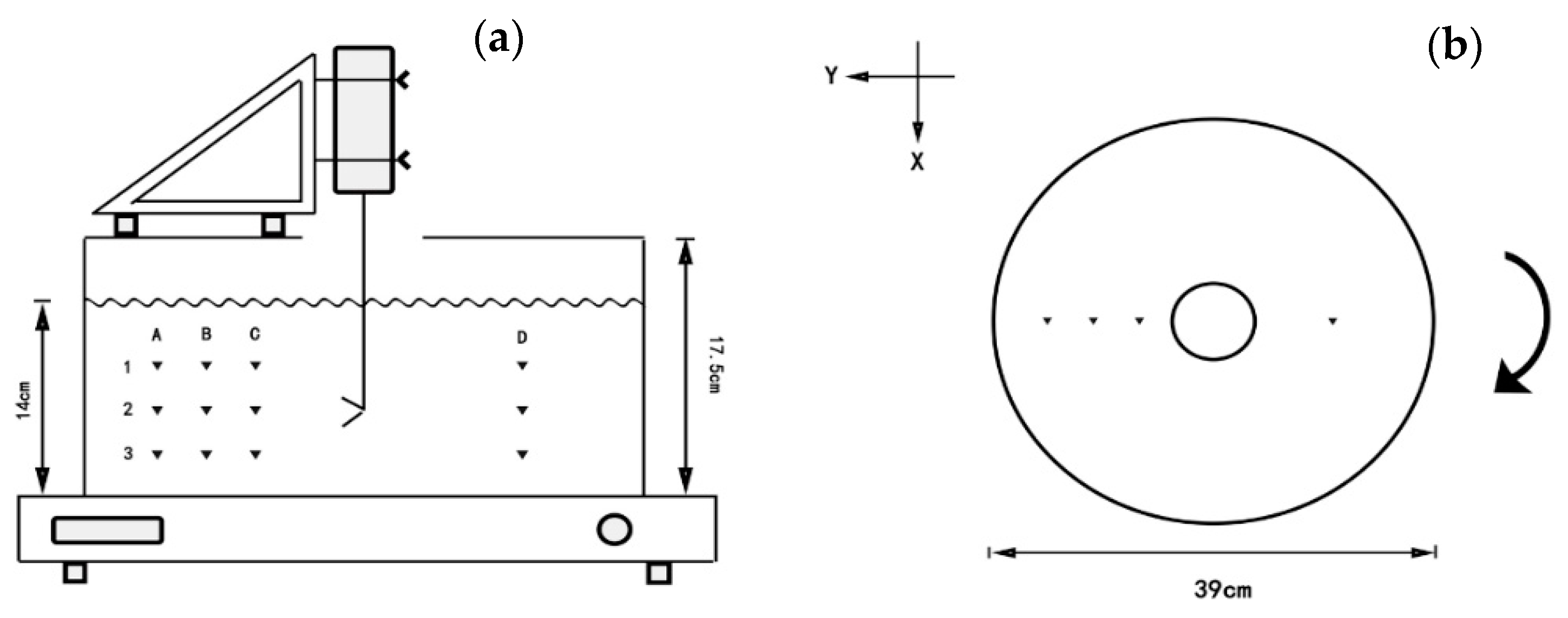
2.1.1. Setup of Orbital Shaker

The turbulence generating system consisted of a customized cylindrical container sitting on an orbital oscillator (GUOHUA HY-8) with an orbital diameter of 2.0 cm (Figure 1a). The height and internal diameter of the container were 17.5 cm and 39 cm, respectively. The water level in the container was 14 cm giving a volume of approximately 16.7 L. The container revolved together with the orbital oscillator following:
X = 0.01 × s i n ( 2 π × 1 T × t )
where X is the displacement, T is the orbital period, and t is the operation time of the orbital oscillator. The horizontal coordinate of the container could thus be expressed as x , y = 0.01 × s i n ( 2 π × 1 T × t ) ,   0.01 × c o s ( 2 π × 1 T × t ) .

2.1.2. Velocity Measurement

A Nortek Vectrino Plus acoustic Doppler velocimeter (ADV, Nortek 6 MHz Vector; Nortek A.S., Vangkroken, Norway) was fixed on a lab-made bracket to directly measure the in situ velocities at 12 sampling points, which were evenly distributed on the vertical section of the diameter of the container (Figure 1a). A rectangular shelf was attached to the orbital oscillator to fasten and mount the ADV probe. The part used to connect the ferrule and shelf was designed as a triangular structure, ensuring the stability of the detector when it rotated. The probe was positioned vertically and placed at least 0.5 cm from the nearest boundary to minimize boundary effects on the measured data. Titanium dioxide (TiO2) was added to water with a suitable concentration to increase signal strength and reduce noise. Three Cartesian flow velocity components could be measured by ADV, with the resolution to be 0.1 mm/s and a velocity bias of   ± 0.5 % . Experimental data for each group were acquired within 15 min at a sampling frequency of 200 Hz. To improve the measurement accuracy, the minimum speed range that met the requirement of speed measurement was adopted.
In this experiment, the range of oscillation frequencies is between 1 and 2 Hz (60–120 rpm), where different rotating speeds, i.e., 60, 80, 85, 90, 100, and 120 rpm, were studied. Three replicated experiments were performed at 90 rpm at a time interval of one week to verify the reproducibility of the device. Each measurement was taken after 10 min of operation when the turbulent motion in the container had reached a steady state. The initial data was then evaluated with the software WinADV (Sontek, San Diego, CA, USA). Correlation and signal-to-noise ratio (SNR) were used to assess the quality of the data. The velocity-time series were used when correlations were >60% and SNR was >20 [42]. In order to reduce the deviation of the Doppler noise of the instrument and manipulate error, the root-mean-square velocity of each component is derived from an average of 15 min velocity data.

2.1.3. Estimation of the Turbulent Kinetic Energy Dissipation Rate

To characterize the turbulence generated in the cylindrical container, we calculated the turbulence dissipation rate (ε) using the following three methods: the energy dissipation law method and the linear regression method based on the measured data of velocity-time series, and the CFD numerical simulation independent of the measured data.
The first method followed the formula described by Taylor [43], assuming that turbulence energy is primarily produced in the largest scales and transferred from large to small eddies until it dissipates around the Kolmogorov microscale. The ε could be described as:
ε = A U r m s 3 l 1
where A is a dimensional constant of order 1 [44], and l is the characteristic size of the largest eddy, commonly assumed to be the length between the orbital diameter and the container diameter in an orbital shaker system [22]. Here, the container diameter was used as l since a vortex with the same diameter as the container was observed during measurement. The root-mean-square velocity ( U r m s ) which helps define the characteristic speed of the turbulence, was calculated using the following formula:
U r m s = u r m s 2 + v r m s 2 + w r m s 2
where
u r m s = μ x 2 μ x 2 n n 1
v r m s = μ y 2 μ y 2 n n 1
w r m s = μ z 2 μ z 2 n n 1
where u r m s , v r m s , and w r m s are the flow fluctuations for Cartesian vectors x, y, and z. n is the number of samples per measurement.
In the second approach, ε was estimated from the energy spectrum, which could be calculated following the linear regression method [45]:
ε = 2 π 10 b B u r m s 2 / 3 3 / 2
where the intersection coefficient b is calculated by fitting a least square regression line with a −5/3 slope to the inertial subrange in a log-log Eulerian energy spectrum, and u r m s = ( u ) 2 ¯ is the root-mean-square of the turbulent component of velocity (u’). B is a non-dimensional universal undetermined constant and was assumed to be 1. The integrated estimate of ε was computed from the logarithmic mean of the dissipation of the three velocity components. The linear regression model used in this study was based on the inertial-advective subrange theory [46], which allows the calculation of turbulence in systems whether or not a net mean flow is larger than the turbulent fluctuations. The model can also filter out the white noise within the instrument and allows the method to estimate dissipation rates in conditions where part of the inertial subrange in the spectrum is below the white noise level. Energy density spectra were derived from 15 min velocity data using the fast Fourier transform (FFT) in the analysis software MatLab®. After that, the energy spectra were smoothed and folded according to the actual situation.
The third method was CFD numerical simulation. All of the equations (Appendix A) in the CFD model were solved by STAR-CCM+ (STAR-CCM+11.02, CD-adapco, Melville, NY, USA), an entire engineering process for solving problems involving fluids or solids, heat transfer, and stress. The RANS (Reynolds Averaged Navier-Stokes equations) k-ε turbulence model was used to simulate the fluid flow and map the distribution of the turbulent dissipation rate (ε) in the orbital oscillation. All of the boundaries are non-slip. The water level, the shape of the orbital shaker, and the temperature were set to be the same as in the laboratory measuring experiment. After comparing the number of meshes (1.06 mil., 0.77 mil., and 0.63 mil.), the asymptotic range of convergence was close to 1 by the GCI method and the final mesh was thus chosen to be 0.63 mil. The time step and inner iterations were set to be 0.01 s and 20, respectively, which assure residual convergence. The solver would run at least 50 s, ensuring the fluid reaches a steady state. To compare with the measuring results, ε that corresponded to the 12 monitoring points in the direct measuring procedure was calculated.

2.2. Application of Orbital Shaker in Biological Culture

2.2.1. Organism and Culture Conditions

Skeletonema costatum is a chain-forming diatom, serving as one of the most important components of coastal phytoplankton communities in temperate and boreal waters. Our experiment obtained Skeletonema costatum from Shanghai Guangyu Biological Technology Co., Ltd., Shanghai, China. (GY-H69, Skeletonema costatum). Using the orbital turbulence generating system, culture experiments of Skeletonema costatum were carried out under three different turbulence conditions at 0 rpm, 60 rpm, and 120 rpm. Other environmental conditions remained the same: in the 0.22 µm-filtered artificial seawater (salinity = 30.5) with f/2 medium at 20 °C, with a light/dark cycle of 12 h/12 h. It should be noted that the volumes of containers used in the culture experiments were smaller (1 L) than the one used for turbulence characterization (~20 L) as described in Section 2.1, which allowed each culture condition to be conducted in triplicate. All of the culture medium and the experimental instruments were sterilized by autoclave (121 °C, 30 min).

2.2.2. Physiological Parameters of Diatom

The culture experiment lasted 13 days, and 120 mL samples were taken every two days to monitor cell density and the chemical composition of the medium. Samples for cell density fixed by Lugol’s iodine solution were pipetted into the planktonic counting plate and counted by an optical microscope. 3 mL of algal liquid solution was filtered through a 0.45 μm glass fiber filter membrane, and the membrane was placed in a 15 mL glass centrifuge tube with an addition of 5 mL of 90% acetone solution. After refrigeration for 24 h, the solution was centrifugated at 3500 r·min−1 for 10 min to obtain the supernatant, and then determined the concentration of Chl. a by fluorospectrophotometry. 15 mL algal liquid solution was poured into a centrifuge tube wrapped with foil and settled in the dark for 2 h to measure Fv/Fm (Mini-PAM-II; WALZ, Effeltrich, German). After filtering through a 0.45 μm cellulose acetate membrane, samples for pH were sealed to minimize the effect of gas-liquid CO2 exchange and determined within 5 h. Samples of [NO3] were sealed and stored under −4 °C, then determined by ion chromatography (ICS-5000+, Thermo, Waltham, MA, USA).

2.2.3. Calculation of the Batchelor Length Scale

The stirring effect of turbulence will stretch the nutrient patches in the water into fine filaments, which will affect the diffusion of nutrients. The smallest length scale of nutrient variation, called Batchelor length scale (ηb) could be estimated as followed:
η b = ν D 2 ε 1 1 4
where ν is the kinematic viscosity of water, and D is the molecular diffusivity of the nutrients [10,47].

2.2.4. Statistical Analysis

Three parallel samples were set under each experimental condition. The mean and standard error of the dependent variable were presented in the results. Statistical analysis of the experimental data was conducted using SPSS statistical software (SPSS Statistics 22.0, IBM, Armonk, NY, USA). We first subjected the data for each group to the Kolmogorov-Smirnov test to verify that they were normally distributed (p > 0.05). Then, to estimate the effect of investigated factors on the analyzed parameters, multifactorial analysis of variance (ANOVA, San Francisco, CA, USA) was applied combined with Tukey’s multiple comparison tests, where statistical significance was set at a 0.05 level.

3. Results and Discussion

3.1. The Exploration of Orbital Oscillator

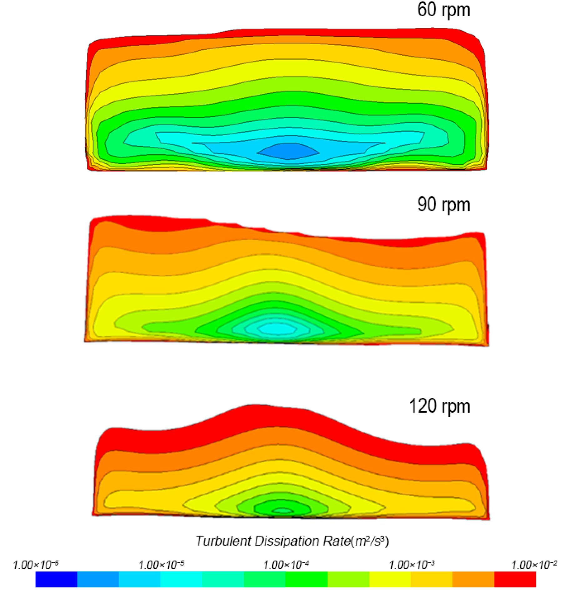
3.1.1. Turbulent Dissipation Rate Distribution

After a fully developed turbulence status had been established, velocity-time series were measured at 12 selected locations at rotation rates from 60 to 120 rpm. The first two mentioned methods could calculate ε at sampling points based on the measured data and compare with the CFD results. According to the CFD simulation results, the turbulence intensity on a cross-section of the container is distributed symmetrically along the axis. We chose position 2B (Figure 1a) as an example to compare the calculation results of the three methods (Table 2), and other points showed a similar trend.
Visual observations of the tank revealed a mean circulation in the tank. The u z , rms / u   x , rms ratios of all measured data were in the range of 0.3 to 0.8, with a mean of 0.57 and a median of 0.56, which confirms the existence of a nearly homogeneous condition in the orbital shaker system. Furthermore, to verify the repeatability of turbulence, three replicate experiments at 90 rpm were performed using the linear regression method. An average   ε of 6.86 × 10⁻³ m2s−3 was measured with a standard deviation of 5.3 × 10⁻⁵, which proved the good repeatability of the orbital oscillator system.

3.1.2. Comparative Analysis of Three Turbulence Simulation Methods

The ε values obtained from three methods showed a similar increasing pattern against the increase in shaking frequency (Figure A1), which indicated a strong relationship between the ε and the shaking frequency of the orbital shaker. When fitted with the least squares linear fitting algorithm, good linearity could be achieved. The linear fitting equations of the three methods were lg ε = 1.824 f 4.751 of the energy dissipation law method, lg ε = 1.930 f 5.119 of the linear regression method, and lg ε = 1.388 f 4.932 of the simulation method, respectively. Based on our experimental results, CFD numerical simulations were in good agreement with the experimental results (the linear regression methods) in the measured rotation rates, which indicated the reliability of the simulation model used in this study.
Although the estimates obtained following linear regression were considered more accurate, its detection range was limited (velocity fields were measured for rotation speeds of 85, 90, 95, and 100 rpm) since part of the inertial subrange in the spectrum was below the white noise level or lack of resolution [45]. On average, the result of the linear regression method was approximately 1.3 times lower than the result of the energy dissipation law method. Differences between the two methods were attributed to misestimating the characteristic length scale l and the universal constant A , implied in the energy dissipation law method. The integral length scale l can be assumed to be between the orbital diameter and the container diameter. If the tank is not large enough, the maximum length scale for turbulent energy could also be limited by the container, which indicates that l in this study may in fact be approximately 39 cm or even larger depending on flow conditions. In this study, when a longer l was used, the turbulence dissipation rates of the two calculation methods would be closer. Comparing the results from measurement and the simulation method, although differences in slope could be observed, the correlation between the simulation method and the linear regression method is approximately 0.93. It indicated that the distribution of turbulent intensity in the containers could be estimated reliable by CFD. Since the CFD simulation method is independent of the measured velocity at the sampling points, it can achieve higher temporal and spatial resolution than the first two methods, which makes it possible to evaluate the turbulence intensity generated by the orbital oscillator in a specific container more conveniently.
Due to the ease of handling and low cost of building and operating, orbital shaker systems are one of the most commonly used bioreactors. However, little research has been carried out to study hydrodynamics in containers on orbital shaker systems, either by direct measurement or numerical simulation. Guadayol et al. [22] measured turbulence in flasks of different shapes (Florence flask, Erlenmeyer flask, Erlenmeyer flask, and Nalgene bottle) and different volumes (1 L and 4 L) with a range of oscillation frequencies between approximately 0.6 to 2 Hz, using a conventional side-looking 1-MHz NDV probe. Zirbel et al. [41] measured the flow field and shear stress in 125 mL Pyrex flasks containing 60 mL of sterile medium using a digital particle image velocimetry (DPIV) system at rotation frequencies of 0.75, 1.25, and 2 Hz and an orbital diameter of 2.54 cm. Kaku et al. [48] compared the turbulence characteristics between baffled (200 mL) and regular (150 mL) Erlenmeyer flasks containing 120 mL of tap water by a hot wire anemometer at rotation frequencies of 2.5 and 3.3 Hz, and an orbital diameter of 1.9 cm. A near-linear relationship between the frequency of a rotation and turbulent dissipation rate ε could be observed by Guadayol et al. [22], although the parameters of the empirical equation differed from ours. The slope and the intercept value of our empirical equation are much lower than Guadayol et al. The main reason is probably due to the size and shape of the containers. The containers used in the Guadayol’s orbital shaker system are from 1 L to 4 L, with the shapes of Florence flask, Erlenmeyer flask and Nalgene bottle. The containers used in Zirbel et al. [41] and Kaku et al. [48] are smaller. Furthermore, the container in Kaku et al. [48] is cone-shaped. The container used in our measurement and simulation is cylindrical, has a 39 cm internal diameter and an approximately 20 L volume. Different corners or irregular shapes at the base would cause different turbulence dissipation rates in containers.

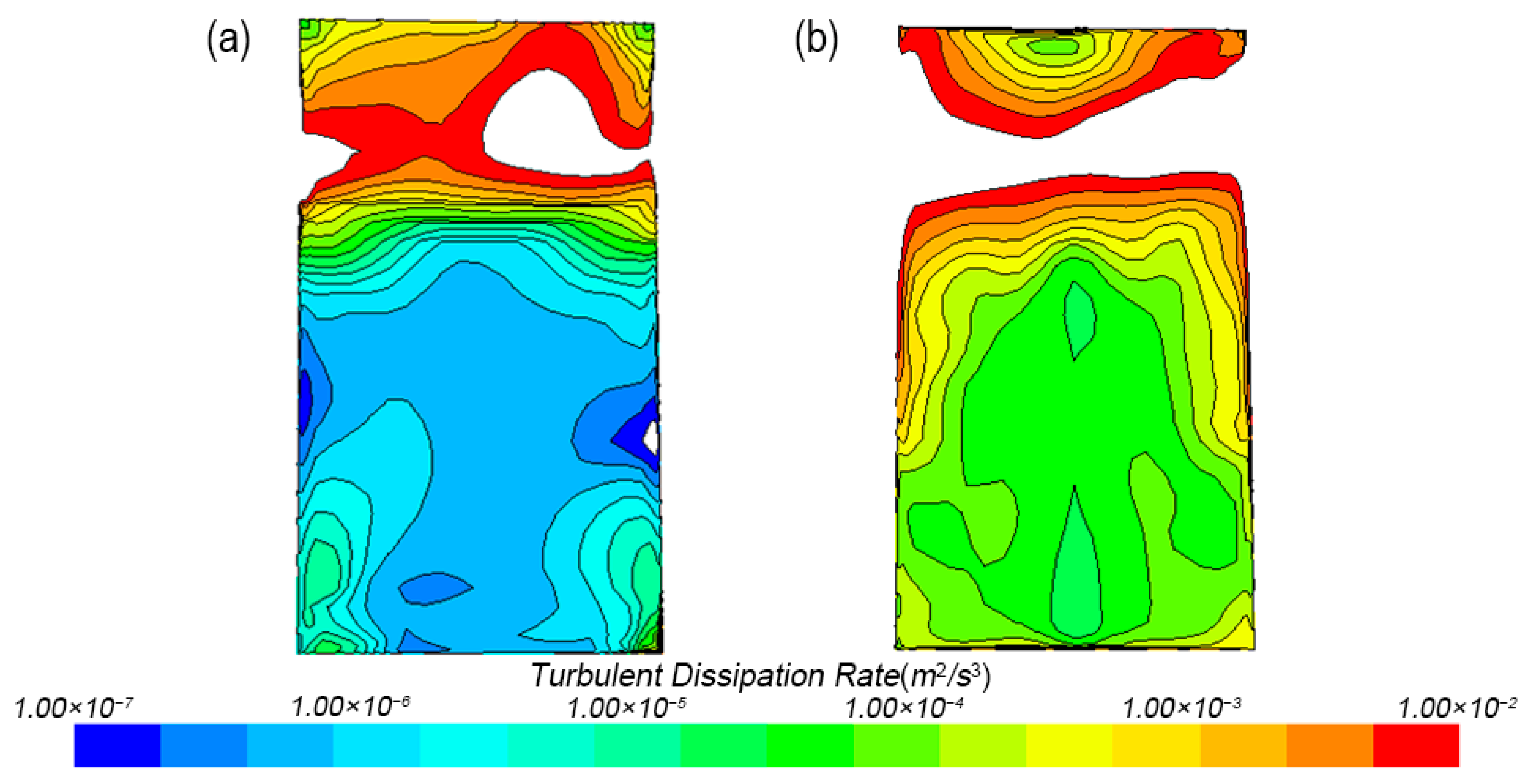
3.1.3. Turbulence Distribution in Tank

A dome-shaped distribution of the dissipation rate was present in the tank, indicating turbulence intensity decreased with increasing distance from the side and bottom walls (Figure 2). The maximum values and most substantial gradients are close to the tank’s surface and periphery. Despite the existence of gradients and the fact that a mean circular horizontal flow was formed within the tank, the energy levels of the whole tank varied spatially, within an order of magnitude, suggesting that the distribution of turbulent kinetic energy dissipation rates in the whole tank could be seen as quasi-homogeneous.
The ε cross-section distributions of different heights were shown in Figure 3. The ε distribution throughout the whole container exhibited axisymmetric and can be divided into three zones. On the bottom, the container was stationary and homogeneous, except for the periphery of the tank. In the middle, the turbulence change trend fluctuated along the horizontal direction but in all exhibited a gentle change and kept in the same order of magnitude. The change in turbulent energy dissipation rates was complex and dramatic at the top due to the liquid level fluctuation. Visual observations and the simulation results of the experiments revealed a mean circular horizontal flow in the tank. Additionally, there was a dominant wave in the horizontal flow, the frequency of which was almost the same as the angular velocity of the walls. Due to the boundary effect, gradients varied dramatically near the periphery of the tank, where the change rate in turbulent energy was approximately three to five times higher than that in bulk.
The distribution of the turbulence was not randomly localized but always located approximately in the same place. Similar turbulence intensity distributions in the container were observed in other researches [25,30,41]. One order of magnitude difference among the mean velocities of three vertically measured positions was reported by Li [25]. Kaku et al. reported a stronger mixing effect at the outer edge near the surface and decreases with depth and/or when approaching the center. The formation of maximum velocity is simulated to occur at the bottom of the higher liquid height side [30].
The orbital shaker system can generate replicable, stable, and relatively homogeneous turbulence. When other parameters of the device keep constant, the turbulence distribution in the container can be easily predicted by the linear fitting equations of the rotation rates and the turbulence intensities. Even though the evaluation results are based on the culture medium without algae, the system could still provide quantifiable, controllable, and repeatable initial turbulence conditions when studying the effects of turbulence on algae growth in the laboratory. However, it is worth noting that the discrepancies in the experimental environment should be considered when extrapolating the real ocean from the laboratory results. Driven by the complex mixing environments and many physical factors, turbulence in the real ocean changes rapidly in time and space, the range of ε covers multiple orders of magnitude, and the flow pattern is complex [49,50,51,52]. In addition, the biologically generated fluid disturbances also affect the mixing [53,54]. So that there is a deviation between the micro-distribution on the surface of algae and the macro measurement data. Since all of the coefficients of k-ε models are obtained for solid surfaces, when exploring the mechanism of turbulence, the turbulence intensity change on the cells’ surface is worthy of further study.

3.2. Cultivation of Skeletonema Costatum with Turbulence

3.2.1. Turbulence Simulation

The batch cultures were carried out in 1 L cylindrical flasks, and the selected rotation rates of orbital oscillation were 0 rpm, 60 rpm, and 120 rpm. The CFD models in the flasks were simulated (Appendix A Figure A2) and the specific turbulence dissipation rate data were shown in Table 3. It is noteworthy that the calculated ηb was much lower than the Kolmogorov length scale and was close to the size of Skeletonema costatum. The possible ε range for the entire ocean, including coastal waters and estuaries, is from 1 × 10 10 m 2 s 3 ~ 1 × 10 2 m 2 s 3 [55]. In the marine environment, such as in a straight lowland river, the intensity range of ε is comparably high with a range of 1 × 10 6 m 2 s 3 ~ 1 × 10 3 m 2 s 3 [56]. Turbulence levels were relatively high in the upper few meters of coastal zones under high wind conditions [57], or in the area affected by the storms and frontal systems in NW Mediterranean coastal waters [58]. Therefore, the corresponding Kolmogorov length scale of these smallest turbulent eddies in nature is usually 300–1000 μm, which is considered only to affect the growth of the large phytoplankton or cell colonies, but has little effect on small algal cells [10,59]. However, ηb matches much of the phytoplankton sizes, revealing that turbulence can affect the nutrient absorption of the smaller phytoplankton. In ecophysiological studies, stronger conditions than those typical in nature were established to help to ascertain the underlying mechanisms of plankton adaptations. Berdalet et al. [3] conducted a relatively high intensity of ε (bulk average, 2.01 × 10 4 m 2 s 3 , range 2.7 × 10 5 m 2 s 3 ~ 2.4 × 10 3 m 2 s 3 ) using an orbital shaker. Orbital shaker systems are adequate for the study of effects of small-scale turbulence on plankton organisms and communities, and especially for plankton with relatively limited mobility and small size.

3.2.2. The Response of Skeletonema Costatum under Different Turbulence Conditions

During the batch culture process, all cultures exposed in different turbulences and still (control) sets exhibited an exponential growth phase in the whole 13 days, although slight moderate slopes could be observed after 2 days in the still set and 6 days in the turbulence-exposed sets. The biomass increased from the original 1.80 ± 0.04 × 10⁵ to the final 16.12 ± 0.51 × 10⁵ cell/mL for still condition, 21.76 ± 0.73 × 10⁵ cell/mL for 60 rpm condition, and 19.40 ± 0.22 × 10⁵ cell/mL for 120 rpm condition, respectively (Figure 4a). Similar trends with turbulence intensity increasing could be observed in the nitrate consumption rate (Figure 4b). Most diatoms can’t move automatically, and have a hard siliceous shell to resist the shear force from outside. Therefore, it is generally believed that diatoms are adaptable to turbulent environment [60], which is also corresponding to the fact that dinoflagellate blooms often occur in long-term calm waters in nature, while diatom blooms often occur after severe disturbance of water [8,61]. Some studies have proved that the uptake rates of nutrients and numbers of diatom cells will increase significantly when the ε was as high as 10−3 m2s−3, although it is sometimes accompanied by the increase of mortality [9,62]. Our results also suggested that the applied turbulence could promote the growth of Skeletonema costatum and that the higher intensity could generally promote higher cell density and nutrient consumption.
The maximum quantum yield (Fv/Fm) of all group decreased at day four, which corresponded well with the pH decrease, indicating an extra reaction occurred which could both decrease the pH in solution and reduce the algae growth. The extra reaction was found to be diatom stimulated CaCO3 precipitation, which was described in more detail in the submitted manuscript. However, the Fv/Fm of the control group showed the lowest values (p < 0.05), which were in accordance with the lowered cell density increase rate (Figure 4c), indicating that under the static condition, the growth of Skeletonema costatum was under extra stress. This stress was probably caused by the diffusion-limited nutrient availability in the still condition. Barton et al. [10] suggested that concentration boundary layers could be generated when the nutrient concentration at the cell surface was reduced by nutrient uptake, which was below that of the bulk medium. The diffusion-limited resource concentration boundary layers enveloping phytoplankton are generally much larger than the cells themselves. Turbulence can be beneficial for phytoplankton growth through changing the diffusive sublayers, which help to support nutrients to the growing cells. Although the application of turbulence promoted the growth and photosynthesis of Skeletonema costatum compared with the still condition, the promotion appeared to be weakened under 120 rpm. It may be attributed to that although diatoms have a certain ability to resist turbulence, excessive turbulence will still cause damage to cells. However, the actual mechanism for the weakening still requires further studies.

4. Conclusions

In this work, three methods, including calculation based on the directly measured velocity and CFD techniques, were coupled to examine the turbulent kinetic dissipation rates and their spatial distributions in an orbital shaker using a range of oscillating frequencies. Relatively homogeneous small-scale turbulence could be formed and cover a range of energy dissipation rates. Although the dominant direction of forcing and radial gradient could be observed in the tank, the differences were kept within an order of magnitude, which indicates the potential of the tank as a well-suited system for studies of plankton interactions, as the turbulence is generated on scales similar to the separation distance between the planktonic particles found in nature. An empirical equation was derived to calculate the dissipation rates for discreet shaking frequencies when all of the other parameters of the shaking devices were kept constant. When the conditions change, the CFD method can also reliably estimate the turbulent intensity distribution in the containers, which could help to quickly assess the average dissipation rate in an orbital shaker system. Also, the low cost, easily-to-handle, and repeatable nature of the orbital shaker made it convenient to explore the effects of turbulence on plankton growth in the lab.
With the practical application of the orbital shaker, the turbulence influence on Skeletonema costatum was experimentally investigated. Turbulence with an appropriate intensity significantly promoted the growth and photosynthetic efficiency of Skeletonema costatum. On account of the heavily silicified frustules of Skeletonema costatum, the damage to the algae cell from shear force generated by turbulence is greatly reduced. On the contrary, turbulence increases the movement of diatoms and enhances the circulation of the water body, which brings a relatively high nutrients to the periphery of the algae continuously, so that the cells can obtain the nutrients more quickly. Later, more studies will be carried out to explore how other planktons respond to the turbulence through the orbital shaker, and the utilization of the orbital shaker has a great prospect.

Author Contributions

Conceptualization, Y.P.; methodology, Z.Y. and L.Y. (Long You); software, Z.Y.; validation, Y.P. and L.Y. (Long You); formal analysis, Z.Y., Y.L. and L.Y. (Long You); investigation, L.Y. (Lin Yu), Y.L. and L.Y. (Long You); resources, W.F. and Y.P.; data curation, Z.Y., Y.L. and L.Y. (Lin Yu); writing—original draft preparation, Y.P. and L.Y. (Lin Yu); writing—review and editing, Y.P., Y.L., Z.-P.J. and L.Y. (Lin Yu); visualization, Z.Y., L.Y. (Lin Yu) and Y.L.; supervision, Y.P., Z.-P.J. and W.F.; project administration, Y.P.; funding acquisition, Y.P. All authors have read and agreed to the published version of the manuscript.

Funding

This research was funded by the National Natural Science Foundation of China (Grant No. 42176036 and 41776084), the Science and Technology Program of Zhoushan City (No. 2022C81002), and the Fundamental Research Funds for the Central Universities (Grant No. 2018QNA4048).

Institutional Review Board Statement

Not applicable.

Informed Consent Statement

Not applicable.

Data Availability Statement

All data are available in the main text or the Appendix A.

Conflicts of Interest

The authors declare no conflict of interest.

Appendix A

The equations can be expressed as follows:
α i = v i v
μ = i μ i α i
ρ = i ρ i α i
where the V i , ρ i and μ i are the volume fraction, density and molecular viscosity of the phase i, respectively. The α i is the transport of volume fractions, which could be expressed in the transport equation:
d d t v α i d V + s α i v v g d a = v S α i α i ρ i D ρ i D t d V  
where S α i is the source or sink of the phase i, and the   D ρ i D t is the Lagrangian derivative of the phase densities ρ i .
STAR-CCM+ is an entire engineering process for solving problems involving fluids or solids, heat transfer, and stress. The Realizable Two-layer K-Epsilon model provided by STAR-CCM+ is suitable for all kinds of y+ values and produces the least inaccuracies for intermediate meshes (1 ≤ y+ ≤ 30) and is used to simulate the fluid flow and map the ε distribution. The transport equations are:
t ρ k + x j ρ k u j = x j μ + μ t σ k k x j + P k + P b ρ Y M + S k
t ρ ε + x j ρ ε u j = x j μ + μ t σ ε ε x j + ρ C 1 S ε ρ C 2 ε 2 k + v ε + C 1 ε ε k C 3 ε P b + S ε
Turbulent viscosity is modeled as:
μ t = ρ C μ k 2 ε
The dilatation dissipation YM is modeled as:
Y M = C M k ε c 2
S is the modulus of the mean strain rate tensor:
S = S = 2 S : S T = 2 S : S
C 1 = max 0.43 , η η + 5
η = S k ε
C 2 = 1.9 , C 1 ε = 1.44 , σ k = 1 C 3 ε = t a n h V b U b
where Vb is the velocity component parallel to g, and Ub is the velocity component perpendicular to g.
Figure A1. Scatter plot of dissipation rate and rotation frequency at position 2B. The dissipation rates were derived from the energy dissipation law method (red circles), the linear regression method (black squares), and the simulation method (blue triangles). The three colored lines represent the least squares linear fitting algorithm for each method.
Jmse 10 01053 g0a1
Figure A2. The CFD model of the culture system at the rotation rates of (a) 60 rpm; (b) 120 rpm.
Jmse 10 01053 g0a2

References

  1. Thorpe, S.A. The Turbulent Ocean; Cambridge University Press: Cambridge, UK; New York, NY, USA, 2005; p. 439. [Google Scholar]
  2. Margalef, R. Life-Forms of Phytoplankton as Survival Alternatives in an Unstable Environment. Oceanol. Acta 1978, 1, 493–509. [Google Scholar]
  3. Berdalet, E.; Peters, F.; Koumandou, V.L.; Roldan, C.; Guadayol, O.; Estrada, M. Species-specific physiological response of dinoflagellates to quantified small-scale turbulence. J. Phycol. 2007, 43, 965–977. [Google Scholar] [CrossRef] [Green Version]
  4. Karp-Boss, L.; Boss, E.; Jumars, P.A. Motion of dinoflagellates in a simple shear flow. Limnol. Oceanogr. 2000, 45, 1594–1602. [Google Scholar] [CrossRef]
  5. Sullivan, J.M.; Swift, E. Effects of small-scale turbulence on net growth rate and size of ten species of marine dinoflagellates. J. Phycol. 2003, 39, 83–94. [Google Scholar] [CrossRef] [Green Version]
  6. Du Puits, R.; Resagk, C.; Thess, A. Thickness of the diffusive sublayer in turbulent convection. Phys. Rev. E 2010, 81, 16307. [Google Scholar] [CrossRef]
  7. Lewis, M.R.; Horne, E.P.W.; Cullen, J.J.; Oakey, N.S.; Platt, T. Turbulent Motions May Control Phytoplankton Photosynthesis in the Upper Ocean. Nature 1984, 311, 49–50. [Google Scholar] [CrossRef]
  8. Huisman, J.; Sharples, J.; Stroom, J.M.; Visser, P.M.; Kardinaal, W.E.A.; Verspagen, J.M.H.; Sommeijer, B. Changes in turbulent mixing shift competition for light between phytoplankton species. Ecology 2004, 85, 2960–2970. [Google Scholar] [CrossRef] [Green Version]
  9. Peters, F.; Arin, L.; Marrase, C.; Berdalet, E.; Sala, M.M. Effects of small-scale turbulence on the growth of two diatoms of different size in a phosphorus-limited medium. J. Mar. Syst. 2006, 61, 134–148. [Google Scholar] [CrossRef] [Green Version]
  10. Barton, A.D.; Ward, B.A.; Williams, R.G.; Follows, M.J. The impact of fine-scale turbulence on phytoplankton community structure. Limnol. Oceanogr. Fluids Environ. 2014, 4, 34–49. [Google Scholar] [CrossRef] [Green Version]
  11. Mackenzie, B.R.; Miller, T.J.; Cyr, S.; Leggett, W.C. Evidence for a Dome-Shaped Relationship between Turbulence and Larval Fish Ingestion Rates. Limnol. Oceanogr. 1994, 39, 1790–1799. [Google Scholar] [CrossRef] [Green Version]
  12. Harkonen, L.; Pekcan-Hekim, Z.; Hellen, N.; Ojala, A.; Horppila, J. Combined Effects of Turbulence and Different Predation Regimes on Zooplankton in Highly Colored Water-Implications for Environmental Change in Lakes. PLoS ONE 2014, 9, e111942. [Google Scholar] [CrossRef] [PubMed]
  13. Edwards, K.F.; Litchman, E.; Klausmeier, C.A. Functional traits explain phytoplankton community structure and seasonal dynamics in a marine ecosystem. Ecol. Lett. 2013, 16, 56–63. [Google Scholar] [CrossRef]
  14. Sengupta, A.; Carrara, F.; Stocker, R. Phytoplankton can actively diversify their migration strategy in response to turbulent cues. Nature 2017, 543, 555–558. [Google Scholar] [CrossRef] [PubMed]
  15. Fraisse, S.; Bormans, M.; Lagadeuc, Y. Turbulence effects on phytoplankton morphofunctional traits selection. Limnol. Oceanogr. 2015, 60, 872–884. [Google Scholar] [CrossRef]
  16. Schapira, M.; Seuront, L.; Gentilhomme, V. Effects of small-scale turbulence on Phaeocystis globosa (Prynmesiophyceae) growth and life cycle. J. Exp. Mar. Biol. Ecol. 2006, 335, 27–38. [Google Scholar] [CrossRef]
  17. Beardall, J.; Raven, J.A. The potential effects of global climate change on microalgal photosynthesis, growth and ecology. Phycologia 2004, 43, 26–40. [Google Scholar] [CrossRef]
  18. Beardall, J.; Stojkovic, S.J.S. Microalgae under Global Environmental Change: Implications for Growth and Productivity, Populations and Trophic Flow. ScienceAsia 2006, 32, 1–10. [Google Scholar] [CrossRef]
  19. Finkel, Z.V.; Beardall, J.; Flynn, K.J.; Quigg, A.; Rees, T.A.V.; Raven, J.A. Phytoplankton in a changing world: Cell size and elemental stoichiometry. J. Plankton Res. 2010, 32, 119–137. [Google Scholar] [CrossRef] [Green Version]
  20. Zhou, J.; Qin, B.Q.; Han, X.X. Effects of the magnitude and persistence of turbulence on phytoplankton in Lake Taihu during a summer cyanobacterial bloom. Aquat. Ecol. 2016, 50, 197–208. [Google Scholar] [CrossRef]
  21. Peters, F.; Marrase, C. Effects of turbulence on plankton: An overview of experimental evidence and some theoretical considerations. Mar. Ecol. Prog. Ser. 2000, 205, 291–306. [Google Scholar] [CrossRef]
  22. Guadayol, O.; Peters, F.; Stiansen, J.E.; Marrase, C.; Lohrmann, A. Evaluation of oscillating grids and orbital shakers as means to generate isotropic and homogeneous small-scale turbulence in laboratory enclosures commonly used in plankton studies. Limnol. Oceanogr. Methods 2009, 7, 287–303. [Google Scholar] [CrossRef] [Green Version]
  23. Bluteau, C.E.; Jones, N.L.; Ivey, G.N. Estimating turbulent kinetic energy dissipation using the inertial subrange method in environmental flows. Limnol. Oceanogr. Methods 2011, 9, 302–321. [Google Scholar] [CrossRef]
  24. Peters, F.; Redondo, J.M. Turbulence generation and measurement: Application to studies on plankton. Sci. Mar. 1997, 61, 205–228. [Google Scholar]
  25. Li, C.; Xia, J.Y.; Chu, J.; Wang, Y.H.; Zhuang, Y.P.; Zhang, S.L. CFD analysis of the turbulent flow in baffled shake flasks. Biochem. Eng. J. 2013, 70, 140–150. [Google Scholar] [CrossRef]
  26. Striebel, M.; Kirchmaier, L.; Hingsamer, P. Different mixing techniques in experimental mesocosms-does mixing affect plankton biomass and community composition? Limnol. Oceanogr. Methods 2013, 11, 176–186. [Google Scholar] [CrossRef] [Green Version]
  27. Amato, A.; Fortini, S.; Watteaux, R.; Diano, M.; Espa, S.; Esposito, S.; Ferrante, M.I.; Peters, F.; Iudicone, D.; Ribera d’Alcalà, M. TURBOGEN: Computer-controlled vertically oscillating grid system for small-scale turbulence studies on plankton. Rev. Sci. Instrum. 2016, 87, 035119. [Google Scholar] [CrossRef] [Green Version]
  28. Kysela, B.; Konfrst, J.; Chara, Z.; Sulc, R.; Jasikova, D. Evaluation of the turbulent kinetic dissipation rate in an agitated vessel. Epj. Web. Conf. 2017, 143, 2062. [Google Scholar] [CrossRef] [Green Version]
  29. Sanford, L.P. Turbulent mixing in experimental ecosystem studies. Mar. Ecol. Prog. Ser. 1997, 161, 265–293. [Google Scholar] [CrossRef] [Green Version]
  30. Kaku, V.J.; Boufadel, M.C.; Venosa, A.D. Evaluation of mixing energy in laboratory flasks used for dispersant effectiveness testing. J. Environ. Eng. 2006, 132, 93–101. [Google Scholar] [CrossRef]
  31. Buchs, J. Introduction to advantages and problems of shaken cultures. Biochem. Eng. J. 2001, 7, 91–98. [Google Scholar] [CrossRef]
  32. Pujara, N.; Du Clos, K.T.; Ayres, S.; Variano, E.A.; Karp-Boss, L. Measurements of trajectories and spatial distributions of diatoms (Coscinodiscus spp.) at dissipation scales of turbulence. Exp. Fluids 2021, 62, 149. [Google Scholar] [CrossRef]
  33. Li, M.; Xiao, M.; Zhang, P.; Hamilton, D.P. Morphospecies-dependent disaggregation of colonies of the cyanobacterium Microcystis under high turbulent mixing. Water Res. 2018, 141, 340–348. [Google Scholar] [CrossRef] [Green Version]
  34. Xiao, Y.; Li, Z.; Li, C.; Zhang, Z.; Guo, J.S. Effect of Small-Scale Turbulence on the Physiology and Morphology of Two Bloom-Forming Cyanobacteria. PLoS ONE 2016, 11, e0168925. [Google Scholar] [CrossRef] [PubMed]
  35. Burns, W.G.; Marchetti, A.; Ziervogel, K. Enhanced formation of transparent exopolymer particles (TEP) under turbulence during phytoplankton growth. J. Plankton Res. 2019, 41, 349–361. [Google Scholar] [CrossRef]
  36. Liu, M.Z.; Ma, J.R.; Kang, L.; Wei, Y.Y.; He, Q.; Hu, X.B.; Li, H. Strong turbulence benefits toxic and colonial cyanobacteria in water: A potential way of climate change impact on the expansion of Harmful Algal Blooms. Sci. Total Environ. 2019, 670, 613–622. [Google Scholar] [CrossRef]
  37. Dell’Aquila, G.; Ferrante, M.I.; Gherardi, M.; Lagomarsino, M.C.; d’Alcala, M.R.; Iudicone, D.; Amato, A. Nutrient consumption and chain tuning in diatoms exposed to storm-like turbulence. Sci. Rep. 2017, 7, 1828. [Google Scholar] [CrossRef]
  38. Ravizza, M.; Hallegraeff, G. Environmental conditions influencing growth rate and stalk formation in the estuarine diatom Licmophora flabellata (Carmichael ex Greville) C.Agardh. Diatom Res. 2015, 30, 197–208. [Google Scholar] [CrossRef]
  39. Bolli, L.; Llaveria, G.; Garces, E.; Guadayol, O.; van Lenning, K.; Peters, F.; Berdalet, E. Modulation of ecdysal cyst and toxin dynamics of two Alexandrium (Dinophyceae) species under small-scale turbulence. Biogeosciences 2007, 4, 559–567. [Google Scholar] [CrossRef] [Green Version]
  40. Yeung, P.; Wong, J. Inhibition of cell proliferation by mechanical agitation involves transient cell cycle arrest at G1 phase in dinoflagellates. Protoplasma 2003, 220, 173–178. [Google Scholar] [CrossRef]
  41. Zirbel, M.J.; Veron, F.; Latz, M.I. The reversible effect of flow on the morphology of Ceratocorys horrida (Peridiniales, Dinophyta). J. Phycol. 2000, 36, 46–58. [Google Scholar] [CrossRef] [Green Version]
  42. McLelland, S.J.; Nicholas, A.P. A new method for evaluating errors in high-frequency ADV measurements. Hydrol. Process 2000, 14, 351–366. [Google Scholar] [CrossRef]
  43. Taylor, G.I. Statistical Theory of Turbulence. Proc. R. Soc. Lond. 1935, 151, 421–444. [Google Scholar] [CrossRef] [Green Version]
  44. Chisita, C.T.; Enakrire, R.T.; Olumide, D.O.; Tsabedze, V.W. Handbook of Research on Records and Information Management Strategies for Enhanced Knowledge Coordination; Information Science Reference: Hershey, PA, USA, 2021; p. 1, online resource. [Google Scholar]
  45. Stiansen, J.E.; Sundby, S. Improved methods for generating and estimating turbulence in tanks suitable for fish larvae experiments. Sci. Mar. 2001, 65, 151–167. [Google Scholar] [CrossRef] [Green Version]
  46. Tennekes, H. Eulerian and Lagrangian Time Microscales in Isotropic Turbulence. J. Fluid Mech. 1975, 67, 561–567. [Google Scholar] [CrossRef]
  47. Taylor, J.R.; Stocker, R. Trade-Offs of Chemotactic Foraging in Turbulent Water. Science 2012, 338, 675–679. [Google Scholar] [CrossRef] [PubMed] [Green Version]
  48. Kaku, V.J.; Boufadel, M.C.; Venosa, A.D.; Weaver, J. Flow dynamics in eccentrically rotating flasks used for dispersant effectiveness testing. Environ. Fluid Mech. 2006, 6, 385–406. [Google Scholar] [CrossRef]
  49. Mackenzie, B.R.; Leggett, W.C. Wind-based models for estimating the dissipation rates of turbulent energy in aquatic environments—Empirical comparisons. Mar. Ecol. Prog. Ser. 1993, 94, 207–216. [Google Scholar] [CrossRef]
  50. Skyllingstad, E.D.; Smyth, W.D.; Moum, J.N.; Wijesekera, H. Upper-ocean turbulence during a westerly wind burst: A comparison of large-eddy simulation results and microstructure measurements. J. Phys. Oceanogr. 1999, 29, 5–28. [Google Scholar] [CrossRef]
  51. Lozovatsky, I.; Roget, E.; Planella, J.; Fernando, H.J.S.; Liu, Z.Y. Intermittency of near-bottom turbulence in tidal flow on a shallow shelf. J. Geophys. Res. Ocean. 2010, 115, c05006. [Google Scholar] [CrossRef] [Green Version]
  52. Tanaka, M. Changes in Vertical Distribution of Zooplankton under Wind-Induced Turbulence: A 36-Year Record. Fluids 2019, 4, 195. [Google Scholar] [CrossRef] [Green Version]
  53. Katija, K. Biogenic inputs to ocean mixing. J. Exp. Biol. 2012, 215, 1040–1049. [Google Scholar] [CrossRef] [PubMed] [Green Version]
  54. Arnott, R.N.; Cherif, M.; Bryant, L.D.; Wain, D.J. Artificially generated turbulence: A review of phycological nanocosm, microcosm, and mesocosm experiments. Hydrobiologia 2021, 848, 961–991. [Google Scholar] [CrossRef]
  55. Yamazaki, H.; Osborn, T.R. In Review of Oceanic Turbulence: Implications for Biodynamics. In Toward a Theory on Biological-Physical Interactions in the World Ocean; Springer: Dordrecht, The Netherlands, 1988; pp. 215–234. [Google Scholar]
  56. Sukhodolov, A.; Thiele, M.; Bungartz, H. Turbulence structure in a river reach with sand bed. Water Resour. Res. 1998, 34, 1317–1334. [Google Scholar] [CrossRef]
  57. Guadayol, O.; Peters, F. Analysis of wind events in a coastal area: A tool for assessing turbulence variability for studies on plankton. Sci. Mar. 2006, 70, 9–20. [Google Scholar] [CrossRef] [Green Version]
  58. Guadayol, O.; Marrase, C.; Peters, F.; Berdalet, E.; Roldan, C.; Sabata, A. Responses of coastal osmotrophic planktonic communities to simulated events of turbulence and nutrient load throughout a year. J. Plankton Res. 2009, 31, 583–600. [Google Scholar] [CrossRef] [Green Version]
  59. Guasto, J.S.; Rusconi, R.; Stocker, R. Fluid Mechanics of Planktonic Microorganisms. In Annual Review of Fluid Mechanics; Massachusetts Institute of Technology: Cambridge, MA, USA, 2012; Volume 44, pp. 373–400. [Google Scholar]
  60. Clarson, S.J.; Steinitz-Kannan, M.; Patwardhan, S.V.; Kannan, R.; Hartig, R.; Schloesser, L.; Hamilton, D.W.; Fusaro, J.K.A.; Beltz, R. Some Observations of Diatoms Under Turbulence. Silicon 2009, 1, 79–90. [Google Scholar] [CrossRef]
  61. Langdon, C. On the causes of interspecific differences in the growth irradiance relationship for phytoplankton. 2. A general-review. J. Plankton Res. 1988, 10, 1291–1312. [Google Scholar] [CrossRef]
  62. Garrison, H.S.; Tang, K.W. Effects of episodic turbulence on diatom mortality and physiology, with a protocol for the use of Evans Blue stain for live-dead determinations. Hydrobiologia 2014, 738, 155–170. [Google Scholar] [CrossRef] [Green Version]
Figure 1. The sketches of the container and experimental devices. (a) The side view of oscillation and measuring device. ▼ marks the sampling points, corresponding to the horizontal (A, B, C, and D) and vertical (1, 2, and 3) indices. (b) The top view of the container. The coordinate system refers to velocity components (u in the x-direction, v in the y-direction, and w in the vertical direction, positively upwards). The arc arrow indicates the rotation direction of the container.
Jmse 10 01053 g001
Figure 2. (a) Contour plot (cross-section view) of the turbulent energy dissipation rates at 90 rpm estimated from (a) the energy dissipation law method and (b) the CFD simulation in the region highlighted in panel (c). ▼ in (c) marks the sampling points, corresponding to the horizontal (A, B, C, and D) and vertical (1, 2, and 3) indices. In order to minimize the errors resulted from extrapolation, panel (a) only presents the results within the sampling region and the data were not extrapolated to boundaries.
Jmse 10 01053 g002
Figure 3. Contour plots of the turbulent kinetic energy dissipation rate distribution of 60 rpm, 90 rpm, and 120 rpm.
Jmse 10 01053 g003
Figure 4. (a) Number of cells; (b) concentration of nitrate; (c) Fv/Fm; (d) pH of Skeletonema costatum during batch culture process under different turbulence intensities. (n = 3, ±SD).
Jmse 10 01053 g004
Table 1. Recent literatures on effects of turbulence on algae.
AlgaeTurbulence Generatorε (m2·s−3)Reference
diatomPaddles10−3–10−1[32]
cyanobacteriumPaddles10−2–10−1[33]
cyanobacteriumPaddles10−3–10−2[34]
diatom
haptophyte
oscillating grids10−6–10−4[35]
natural communitiesoscillating grids10−3–10−2[36]
diatomoscillating grids105[37]
Zygnematophyceae
Bacillariophyceae
Chlorophyceae
Prasinophyceae
oscillating grids10−5–10−3[15]
prymnesiophyceaeoscillating grids10−6–10−4[16]
dinoflagellatesoscillating grids10−8–10−4[5]
diatomorbital shaker-[38]
dinoflagellatesorbital shaker10−5–10−2[39]
dinoflagellatesorbital shaker10−4[3]
diatomorbital shaker10−3[9]
dinoflagellatesorbital shaker10−5–10−4[40]
dinoflagellatesorbital shaker10−5–10−4[41]
Table 2. Comparisons of the turbulent dissipation rates ( ε ,   m 2 s 3 ) at different rotation frequencies at position 2B using three methods.
Rotation Rate
(rpm)
Frequence
(Hz)
The Energy Dissipation Law MethodThe Linear Regression MethodThe Simulation Method
601.000 1.90 × 10⁴
701.1671.83 × 103 4.35 × 10⁴
801.3332.72 × 103 1.07 × 10³
851.4177.16 × 103 3.97 × 10³ 1.31 × 10³
901.5001.63 × 102 6.86 × 10³ 2.04 × 10³
951.5832.28 × 102 7.38 × 10³
1001.6672.41 × 102 1.33 × 10² 2.85 × 10³
1101.8334.68 × 102 3.65 × 10³
1202.0004.20 × 102 4.94 × 10³
Table 3. The turbulence parameters of batch cultures at different rotation rates.
Rotation Rate60 rpm120 rpm
Frequency (Hz)1.0002.000
ε (m2·s−3)2.4 × 10−75.2 × 10−5
The Kolmogorov length scale ( η k , μm)143335
The Batchelor length scale ( η b , μm)3749
Publisher’s Note: MDPI stays neutral with regard to jurisdictional claims in published maps and institutional affiliations.

