Prediction of Wave Energy Flux in the Bohai Sea through Automated Machine Learning

Abstract

The rational assessment of regional energy distribution provides a scientific basis for the selection and siting of power generation units. This study, which focused on the Bohai Sea, set 31 research coordinate points in the Bohai sea for assessing the potential/trends of wave energy flux (WEF). We applied a point-to-point time series prediction method which modelled the different geographical coordinate points separately. Subsequently, we evaluated the performance of three traditional machine learning methods and three automated machine learning methods. To estimate WEF, the best model was applied to each research coordinate points, respectively. Then, the WEF was calculated and predicted based on the data of MWP, SWH, and water depth. The results indicate that, for all coordinates in the Bohai Sea, the H2O-AutoML algorithm is superior to the other five algorithms. Gradient boosting machine (GBM), extreme gradient boosting (XGBoost), and stacked ensemble models yielded the best performance out of the H2O algorithms. The significant wave height (SWH), the mean wave period (MWP), and the WEF in the Bohai Sea tended to be concentrated in the center of the sea and dispersed in the nearshore areas. In the year 2000, 2010, 2020, and 2030, the maximum annual average WEF at each research coordinate in the Bohai Sea is around 1.5 kW/m, with a higher flux in autumn and winter. In summary, the results provide ocean parameter characterization for the design and deployment of wave energy harvesting devices. Moreover, the automated machine learning introduced herein has potential for use in more applications in ocean engineering.

1. Introduction

The creation and exploitation of renewable energy are receiving increasing attention in relation to realizing carbon neutrality and carbon peaking [1,2,3,4,5]. The ocean comprises 71% of the earth’s surface and stores an enormous amount of energy. Wave energy, current energy, tidal energy, salinity gradient energy, and other types of ocean energy are extensively available [6,7,8]. Wave energy is a clean, sustainable energy source that does not emit carbon dioxide. Moreover, the motion of the waves never stops, day or night, and utilizing wave energy does not take up land space. Usually, large electromagnetic generators (EMGs) are used for wave power generation [9]; common wave energy converters (WECs) include nodding duck, oscillating water column, pendulum, and floating oscillating devices, amongst others [10,11]. For example, Wu et al., proposed a mechanical power take-off system (PTO) that is integrated with both a flywheel and spiral springs [12]. Cai et al., proposed a tunable energy harvesting device based on a two-mass pendulum oscillator [13]. Li et al., proposed a two-body self-floating oscillating surge wave energy converter which relieves more reaction forces on the mooring lines [14]. It is difficult for large devices to fully adapt to the randomness of waves. Utilizing traditional wave energy harvesting devices has always been one of the challenges faced by researchers [15]. In 2012, Wang et al., proposed triboelectric nanogenerators (TENGs) based on Maxwell displacement current [16]. As compared to conventional EMGs, TENGs are more effective at capturing energy at low frequencies (typically defined as 0.1–3 Hz) [17]. Subsequently, in 2014, the concept of using a TENG network to harvest blue energy was proposed [18]. TENG offers the advantages of being inexpensive, light, and simple to expand. The TENG grid-based distributed architecture is better suited to collecting high-entropy wave energy, which is a fundamentally different approach of obtaining renewable energy from the ocean [19,20].

The target deployment and effective operation of wave energy converters requires reliable wave assessment. Therefore, it is particularly important to evaluate the area of interest before the development of renewable energy sources. Wave energy flux (WEF), otherwise known as wave energy power density, is an important metric used to evaluate the wave energy potential of the sea area. However, the evaluation of large-scale energy is extremely challenging in terms of both the theoretical calculation and operational practice. Small-scale evaluations are carried out first in the evaluation process of other clean energy sources, such as wind and solar energy. For example, Dvorak used high-resolution mesoscale weather modeling data to assess wind energy in the California region [21]. Wan et al., conducted a joint assessment of wave and wind energy in the South China Sea based on ERA-Interim data [22]. Liu et al., employed a geographic information system (GIS), which analyzes spatial and dynamic geographic information, to assess solar energy in the Jiangsu region of China [23]. Dasari et al., conducted a high-resolution analysis of solar energy in the Arabian Peninsula region [24]. Odhiambo et al., assessed solar energy in the Yangtze River Delta region [25]. For wave energy assessment, Iglesias assessed the wave energy potential of the Galicia region using a third-generation ocean wave model [26]. Wang et al., worked on the prediction of the SWH in the South China Sea using the multiple sine function decomposition neural network (MSFDNN) method [27]. Sierra used numerical modeling to assess the wave energy power off the Atlantic coast of Morocco [28].

This study focuses on the Bohai Sea, which is the largest inland sea in China and is surrounded by the Shandong Peninsula and the Liaodong Peninsula. As an inland sea, the Bohai Sea has a relatively weak self-purification ability, and pollution discharges from inland easily stagnate in the sea area [29]. The Bohai Sea is located in the core urban agglomeration in northern China, with a huge urban energy demand. The rational assessment and utilization of marine renewable energy is of great significance to the construction of a green energy cycle mechanism in the surrounding area.

The concept of machine learning prediction is to use a model to learn specific patterns or relevancies in the training set in order to make predictions. Regression and classification are the two major types of prediction [30]. Supervised learning, unsupervised learning, and semi-supervised learning make up the three modes of machine learning. Traditional machine learning models include logistic regression (LR) [31], support vector machine (SVM) [32], extreme gradient boosting (XGBoost) [33], k-nearest neighbor (KNN) [34], random forest (RF) [35], and asymptotic regression (AR) [36]. However, traditional machine learning usually requires complex feature engineering and cannot be applied in certain cases. Subsequently, deep learning algorithms solve the shortcomings of classic machine learning models in feature engineering. Some deep learning models include artificial neural networks [37], recurrent neural networks (RNNs) [38,39], convolutional neural networks (CNNs) [40,41], long short-term memory (LSTM) [42], ResNet [43], a group method of data handling (GMDH) [44], and vision transformers (ViTs) [45]. Although the deep learning algorithm model is powerful and complicated, it depends, to a certain extent, on the magnitude of the dataset, and can perform poorly on small sample problems. Moreover, for a single problem, a specific model algorithm will usually suffice, but, when solving multiple parallel problems simultaneously, very few algorithms meet the requirements of all the problems [46]. For example, in geospatial space, it is difficult to explain the data patterns of sites in different geographical locations using only one specific algorithm. Because parallel problems usually have different levels of reciprocity, one single algorithm cannot meet the application requirements, even if it sacrifices the fitting accuracy of one single problem. Therefore, when solving multiple parallel problems simultaneously, trying to isolate the analysis in different problems using multiple algorithms can help to achieve global accuracy. Automated machine learning refers to the automatic training and prediction of input data with fixed computational resources, which can be used to automatically find the best model algorithm for one single problem and multiple parallel problems. Automated machine learning performs a nested search to explore the best model: the outer search is used to select the type of machine learning algorithm and the inner search is used to optimize the hyperparameters of the selected algorithm model. Random search [47], grid search [48], and Bayesian optimization [49] are commonly used hyperparameter optimization strategies. Many studies employ automated machine learning to carry out work in related fields. Sun et al., for example, reconstructed Gravity Recovery and Climate Experiment (GRACE) total water storage using automated machine learning [46]; Koh et al., used automated machine learning for plant phenotyping [50]; COVID-19 deaths were modeled using a Kalman Filter and automated machine learning methods by Han et al. [51]; and Liu et al., used a new automated machine learning technique to explore the factors affecting blood lead levels in children [52].

According to previous research, the feasibility of automated machine learning methods in assessing the WEF has not been demonstrated, and the majority of researchers still utilize a single algorithm and not automated machine learning methods to solve practical problems. The aim of this study was twofold. First, we attempted to construct a workflow for energy calculation and prediction by deriving the WEF from physical parameters of the ocean surface. Second, we aimed to apply automated machine learning to highlight the impact of data spatial variability at different coordinates on model selection.

Our research contributions are as follows:

• Apply a method for time series point-to-point prediction.
• Compare models of traditional machine learning and automated machine learning in the scenario of wave energy prediction.
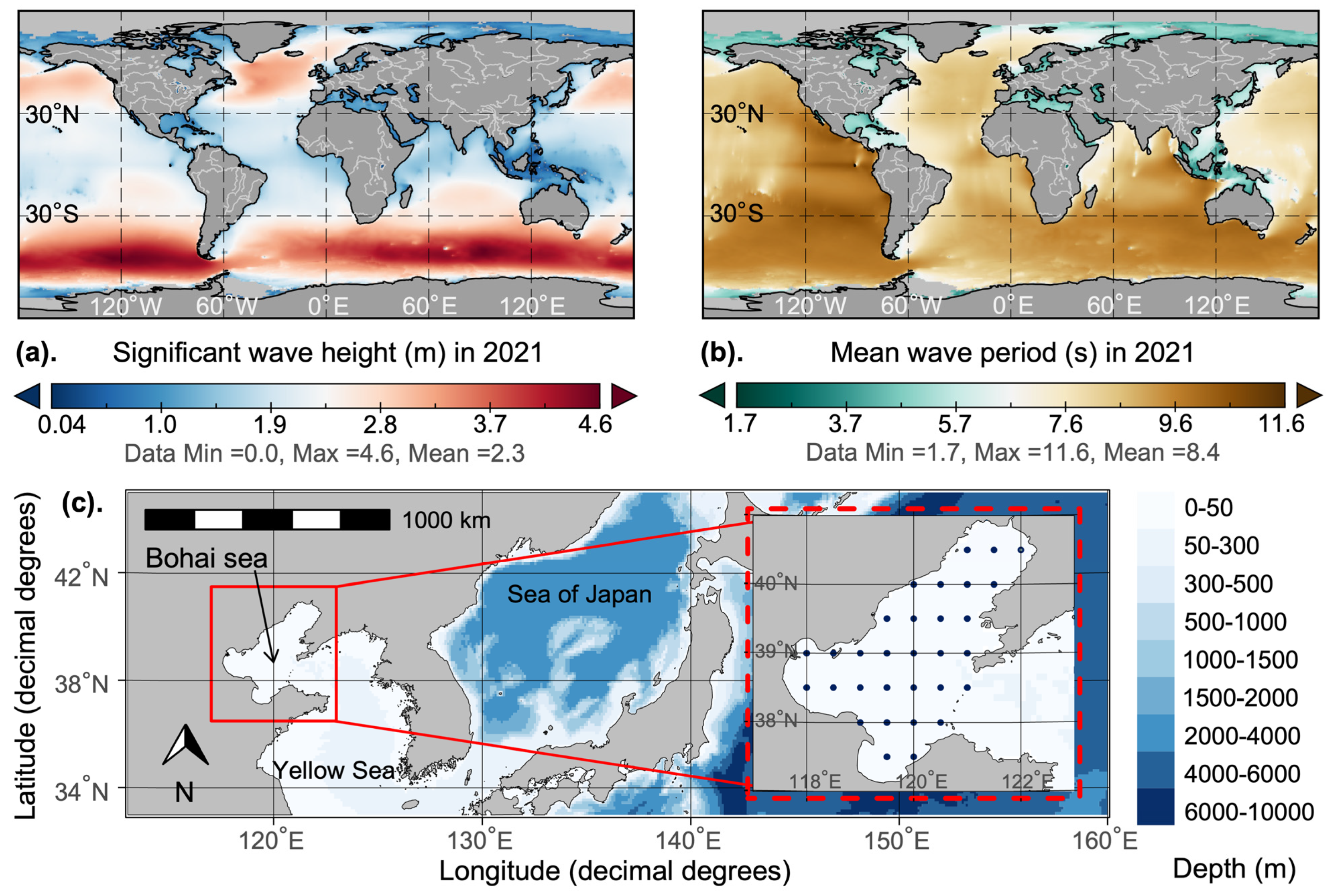
• Predict significant wave height, mean wave period, and wave energy flux of the Bohai Sea, which provides ocean parameters theoretical characterizations for the wave development in the Bohai Sea.

To summarize, in this study, on the basis of ERA5 data, six machine learning algorithms (including three conventional and three automatic machine learning algorithms) were applied to predict and evaluate the SWH, MWP, and WEF in the Bohai Sea 10 years into the future. Section 2 presents the data sources and model prediction workflow. Section 3 shows the related results and discussion, and Section 4 concludes the study.

2. Materials and Methods

The outline of this study is shown in Figure 1. As one can see, it is divided into data processing, statistical analysis, model prediction, and energy calculation. This section describes each part in detail.

2.1. Data

The basic data were obtained from the ERA5 dataset of the European Centre for Medium-Range Weather Forecasts (ECMWFs) [53,54]. ERA5 is a global reanalysis dataset with different spatial resolutions from 0.25° × 0.25° to 1° × 1°. Wang et al., analyzed the high compatibility of wave data from ERA5 with data recorded by indigenous buoy sensors [55]. Wang et al., analyzed the North American Atlantic and Pacific buoy observations with ERA5 wave data and found a strong correlation coefficient between them [56]. Wang et al., performed the same comparative work in the South China Sea and reported good agreement [57]. Mahmoodi et al., verified that ERA5 reanalysis data are closely related to observations in the study area [58]. GEBCO gridded bathymetric data were obtained from the British Oceanographic Data Centre (BODC) as bathymetric data [59,60].

The ERA5 data product used in this study is the monthly averaged reanalysis, with variables including the SWH and MWP. The time dimension is from January 1979 to December 2021 (data from 516 months) and the spatial dimension is 37° N–40.5° N, 118° E–122° E. The resolution is 0.5° × 0.5°, so there are 31 research coordinate points in the Bohai Sea. The original ERA5 data were downloaded and saved in netCDF format, and then locally converted to the csv format data. After data cleaning and archiving, each coordinate point had 516 months data in two variables.

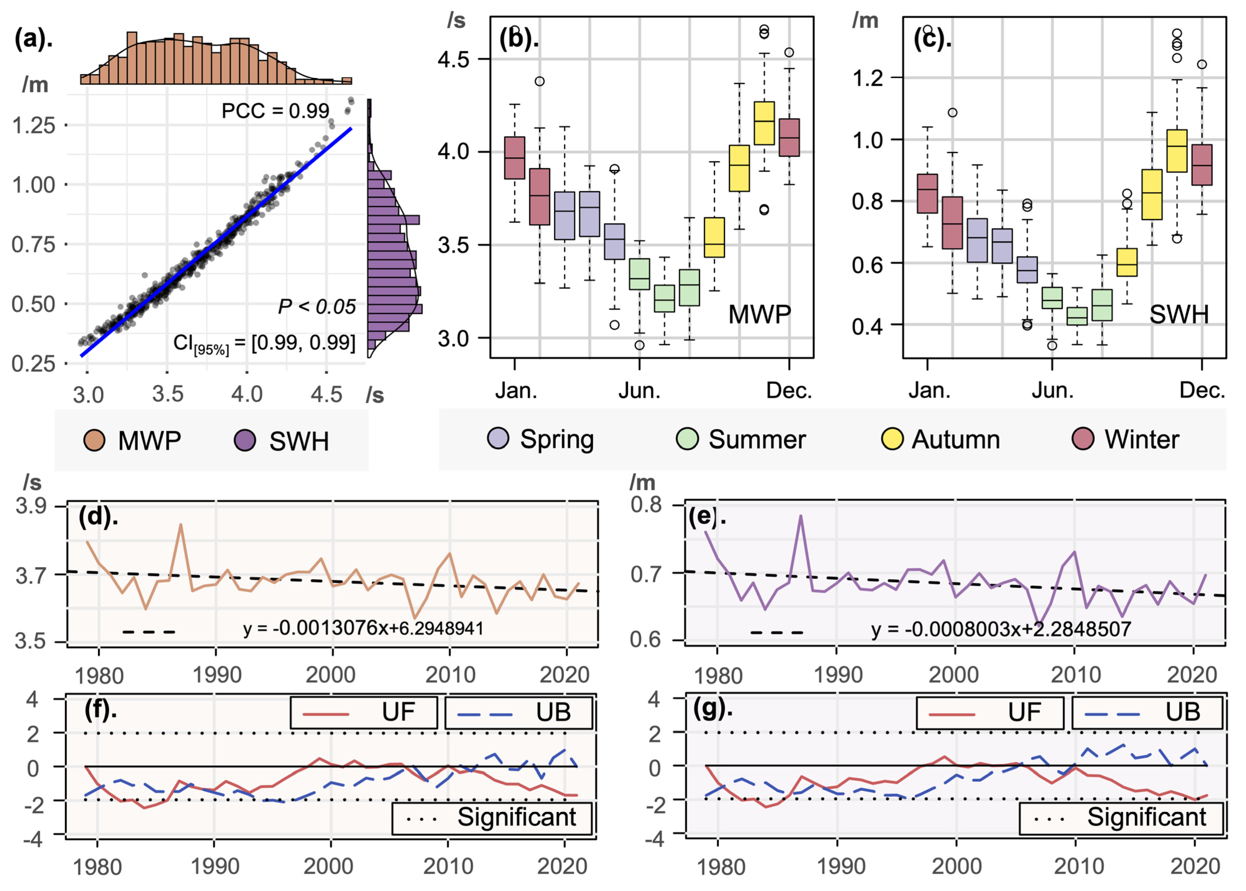
2.2. Mann–Kendall Test

The Mann–Kendall test is a nonparametric statistical method commonly used in meteorology, which can effectively distinguish whether a natural change process belongs to a natural fluctuation or a certain change trend [61,62,63]. For a timeseries x with n samples, the order column $S_{k }\mathrm{is} \mathrm{first} \mathrm{constructed}$:

$$S_k=\sum _{i=1}^k{r}_{i,}\left(k=2,3,\dots ,n\right)$$

(1)

$$r_i=\left\{\begin{array}{ll}+1\hfill & x_i>x_j\hfill \\ 0\hfill & x_i\le x_j\hfill \end{array}, \left(j=1,2,\dots ,i\right)\right.$$

(2)

Thereafter, statistic $U{F}_k$ is defined as follows:

$$U{F}_k=\frac{S_k-E\left(S_k\right)}{\sqrt{Var\left(S_k\right)}},\left(k=1,2,\dots ,n\right)$$

(3)

where the expectation $E\left(S_k\right)$ is the mean of $S_k$ and $Var\left(S_k\right)$ is the variance of $S_k$:

$$E\left(S_k\right)=\frac{n\left(n+1\right)}{4}$$

(4)

$$Var\left(S_k\right)=\frac{n\left(n+1\right)\left(2n+5\right)}{72}$$

(5)

The statistic $U{F}_k$ is calculated by the positive order of time series x, with $U{F}_1$ = 0. Conversely, the statistic $U{B}_k$ is calculated according to the reverse order of x as $U{B}_1$ = 0. A $UF$ greater than 0 indicates that the sequence has an upward trend, while a $UF$ of less than 0 indicates a downward trend. If the significance level α is given, when |$U{F}_k$| > $U_{\alpha }$, it indicates that there is a significant trend change in the time series; in particular, when α = 0.05, $U_{\alpha }$ = ±1.96 in the standard normal distribution [64]. When the statistics $UF$ and $UB$ intersect within the significant level range, the intersection point is the mutation point of the sequence.

2.3. Forecast

In order to predict the MWP and SWH in the sea area to calculate the WEF, we employed conventional machine learning, automated machine learning, and automated deep learning, respectively. This section describes the data processing in detail and the models.

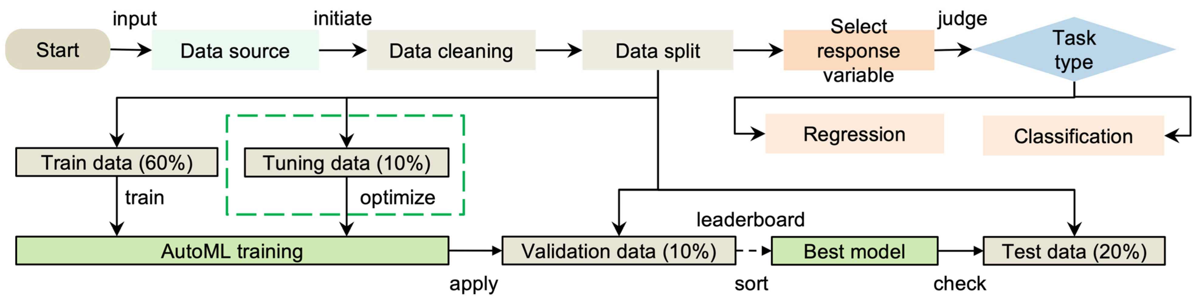
2.3.1. Data Processing

Before time series data were input into the model for training and prediction, feature engineering (time series features) was performed to expand the one-dimensional time series data into multicolumn feature data. The one-dimensional time series data were split into training and testing data in 8:2 ratio. The extended features were classified according to annual seasonality, weekly seasonality, daily seasonality, and weekly cyclic patterns to form 23 columns of matrix data, such as year, month, quarter, day of the week, day of the month, day of the year, week of the month, day of the month, day of the week, hour, minute, and second.

2.3.2. Conventional Machine Learning Models

For conventional machine learning models, we performed R packages of forecast (8.16), ATAforecasting (0.0.56), and forecastHybrid (5.0.19). ATAforecasting is a new method for automatic time series forecasting (to replace exponential smoothing and ARIMA) that uses the Ata method with Box–Cox power transformations and seasonal decomposition techniques [65,66,67,68]. ForecastHybrid uses seven models of auto.arima, ets, thetaf, nnetar, stlm, tbats, and snaive. The results of the seven models were integrated into an equally weighted manner for forecasting [69,70,71,72,73]. The error metric was set to the root mean square error (RMSE), and parallel computing was turned on. R package forecast was used for auto ARIMA, which returned the best ARIMA model based on the AIC or BIC metrics [74,75,76].

2.3.3. Automated Machine Learning Models

For automated machine learning, we employed the R packages H2O (3.36.0.1) and Rminer (1.4.6). H2O is an open-source scalable machine learning platform, and the R package of the same name is used to connect H2O instances on the R platform. H2O-AutoML is the supervised learning algorithm [77] and is referred to as H2O in the following. The regression models available in H2O include the generalized linear model (GLM) [78], the deep neural network (DNN) [79], the gradient boosting machine (GBM) [80], extreme gradient boosting (XGBoost) [81], the distributed random forest (DRF), the extreme random tree (XRT) [82], and two stacked ensemble (SE) models, wherein the stacked ensemble models are supervised ensemble machine learning methods [83,84]. One class of H2O’s ensemble models uses all trained models, and the other class only uses the best performing models from each family of algorithms. H2O-AutoML uses the grid search method for hyperparameter tuning (tuning one hyperparameter in GLM, seven hyperparameters in DNN, eight hyperparameters in GBM, nine hyperparameters in XGBoost, the untuned hyperparameters in XRT, and the ensemble model’s parameter).

Figure 2 shows the outline flow for using H2O-AutoML. Users first need to prepare basic data and perform data cleaning. It is worth noting that when H2O-AutoML starts training, it will check the data quality again and automatically discard or delete useless data. Then, the data need to be divided into 4 kinds of data: the training set, the tunning set, the validation set, and the test set. We made divisions according to the ratio of 6:1:1:2. The tunning data were used to adjust the hyperparameters of each model internally to prevent overfitting or underfitting. The training set, the tunning set, and the validation set are usually the actual training sets in a broad sense. After feeding the necessary data, H2O-AutoML starts training and hyperparameter tuning, and the best model is picked, which is highly automated and requires no user involvement. Training is stopped by setting a maximum runtime or a maximum number of models. All internally trained models are tested on the validation data, and the leaderboard of the model is generated at the same time. We only utilized the best performing model for subsequent prediction work. It is worth noting that the test data were only used once and should not be used directly or indirectly during model training. The maximum running time of each model was set at 20 min, and deviance was selected as the stop indicator.

Rminer is an automated machine learning algorithm package on the native R platform that allows users to define machine learning models for search, hyperparameter ranges, and stopping metrics [85,86]. In this study, we used the generalized linear model (GLM) [78], Gaussian kernel support vector machines (SVMs) [87], shallow multilayer perceptron (MLP), random forest tree (RF) [88], extreme gradient boosting (XGBoost) [81], and ensemble models, which use the best performing model from each algorithm family. Rminer utilizes the grid search method to reconcile two hyperparameters in GLM, three hyperparameters in SVM, one hyperparameter in MLP, one hyperparameter in RF, one hyperparameter in XGBoost, and two hyperparameters in the ensemble model. The maximum number of searches for hyperparameter adjustment was set to 100, and the number of model fitting runs was set to 50. After training, the H2O and Rminer-dominant programs recorded the individual model scores. We focused solely on the optimal model.

2.3.4. Automated Deep Learning Models

We used H2O and Autokeras for automated deep learning. In the deep learning scenario, H2O uses a fully connected multilayer artificial neural network trained by a stochastic gradient descent back-propagation algorithm. The H2O-AutoML tuning hyperparameters include the dropout ratio of the input and hidden layers, the number of hidden layers and hidden units per layer, the learning rate, the number of training epochs, and the activation function. Autokeras is an automatic deep neural architecture search (NAS) tool with the ability to automatically tune hyperparameters including units, activation functions, dropout rates, etc. Unlike the H2O, Autokeras uses Bayesian optimization for model selection. Autokeras provides deep learning models including LSTM [42] and GRU [89], and the AutoModel class, which combines HyperModel and Tuner to tune the model, was used in this work. Put simply, the inputs and outputs are specified, and AutoModel automatically explores the rest.

2.3.5. Experimental Conditions

The software environment for the three conventional machine learning algorithms and Rminer was macOS Monterey 12.1, R 4.1.1 (64 bit), Rstudio 1.4.1717, and the hardware environment was 8 G RAM, Apple M1 chip. The software environment for H2O was Ubuntu 18.04, R 4.1.1, and the hardware environment was 160 G RAM 32-core Intel Xeon Platinum 8260 L CPU 2.30 GHz. The software environment for the Autokeras model was Ubuntu 18.04, Python 3.8, CUDA 11.0, cuDNN 8.0, Tensorflow 2.4, Keras 2.3.1, and autokeras 1.0.16.post1, and the hardware environment was 64 GB RAM, NVIDIA GeForce RTX 3080 Ti 12 GB, and 8-core Intel Xeon CPU E5-2686 v4 2.30 GHz. The SWH and MWP were two research variables, and the 31 study coordinate points in the Bohai Sea were trained for all the six models above, i.e., a total of 372 (2 × 31 × 6) generalized model training processes (some models integrate multiple models training processes internally). At each coordinate point, we comprehensively considered the RMSE and MAPE indicators to select the best model (prediction model) for that point.

2.4. Wave Energy Flux Calculation

The wave energy flux, also known as the wave energy power density, is one of the most important characteristic quantities for evaluating the distribution of wave energy. Ocean waves are composed of many wave components, and each component wave has its own parameters such as height, period, and direction. In reality, the number of waves interacting with ocean waves is huge. In order to evaluate the wave energy in complex sea conditions, the SWH and energy period are used to calculate the WEF. The formula is as follows:

$$P_w \left(\mathrm{kW}/\mathrm{m}\right)=\frac{\rho g^2}{64\pi }{H}_S^2{T}_e\approx 0.5H_S^2{T}_e$$

(6)

where $\rho$ is the seawater density, $g$ is the gravitational acceleration constant, $H_s$ is the effective wave height, and $T_e$ is the energy period. This formula is widely used for estimating the WEF; however, there are times when wave energy is often overestimated, especially in shallow water [90]. The average water depth of the Bohai Sea is 18 m, so the water depth factor must be considered when calculating the WEF. Liang et al., proposed a general WEF calculation formula suitable for shallow water and deep water. By introducing the water depth parameter h, the estimation accuracy in different water depths was improved [90]. The formula is as follows:

$$P_w=\frac{\pi \rho gh{H}_s^2}{16T_e}\left[\frac{1}{\mu }+\frac{2}{\sin \mathrm{h}\left(2\mu \right)}\right]$$

(7)

Subsequently, Mahmoodi improved on Formula (7) with a new dispersion equation ${\mu }_B$ proposed by Beji [91], as shown in Formula (8), and a simple explicit approximation to the dispersion equation proposed by Simarroa et al. [92], as shown in Equation (9):

$${\mu }_B=\frac{{\mu }_0\left[1+{\mu }_o^{1.09}{e}^{-\left(1.55+1.30{\mu }_0+0.216{\mu }_0^2\right)}\right]}{\sqrt{\tan \mathrm{h}\left({\mu }_0\right)}}$$

(8)

$${\mu }_{*}=\frac{{\mu }_B^2+{\mu }_0{\cos \mathrm{h}}^2\left({\mu }_B\right)}{{\mu }_B+\sin \mathrm{h}\left({\mu }_B\right)\cos \mathrm{h}\left({\mu }_B\right)}$$

(9)

$${\mu }_0=k_{0}h=\frac{2\pi }{L_0}=\frac{{\omega }^{2}h}{g}=\frac{4{\pi }^{2}h}{g{T}^2}\approx \frac{4{\pi }^{2}h}{g{T}_e{}^2}$$

(10)

where ${\mu }_0$ is the dispersion parameter, $k_0$ is the deep-water wave number, $\omega$ is the wave angular frequency, $L_0$ is the deep water wave length, $g$ is the gravitational acceleration constant, and $h$ is the water depth. Thus, the final WEF evaluation equation is as follows:

$$P_w=\frac{\pi \rho gh{H}_s^2}{16T_e}\left[\frac{1}{{\mu }_{*}}+\frac{2}{\sinh \left(2{\mu }_{*}\right)}\right]$$

(11)

It can be seen that the error in the WEF is mainly influenced by the SWH, which is due to the fact that the WEF is proportional to the square of the effective wave height [93]. However, there is no agreement on the wave period, which is the most representative metric regarding the sea state. The wave period in Formula (11) is defined as the energy period, and the MWP in ERA5 data are the average time of two consecutive wave crests passing a fixed point on the ocean surface, corresponding to the energy period. The water depth data were obtained from the GEBCO gridded data [59,60].

2.5. Statistical Metrics

In the correlation analysis, we used Pearson correlation coefficient (PCC) to measure the closeness of the association between the two datasets. PCC takes the value range of [−1, 1], i.e., greater than 0 demonstrates a positive correlation and less than 0 demonstrates a negative correlation. The mathematical formula is as follows, where $\overline{X}$ is the average of all variables $x_i$ and $\overline{Y}$ is the average of all variables $y_i$.

$$\mathrm{PCC}=\frac{{\sum }_{i=1}^N\left(x_i-\overline{X}\right)\left(y_i-\overline{Y}\right)}{\sqrt{{\sum }_{i=1}^N{\left(x_i-\overline{X}\right)}^2{\sum }_{i=1}^N{\left(y_i-\overline{Y}\right)}^2}}$$

(12)

For model accuracy assessment, we applied two accuracy assessment metric CCCs, RMSE and MAPE, where $x_i$ was defined as the true value and $y_i$ as the predicted value, with a total of $N$ pairs of data. The concordance correlation coefficient (CCC) contains the function of the Pearson correlation coefficient (while considering more factors including intercept) and is an indicator that can measure both the correlation and absolute difference. The formula is as follows:

$$\mathrm{CCC}=\frac{2s_{xy}}{s_x^2+s_y^2+{(\overline{X}-\overline{Y})}^2}$$

(13)

$$s_x^2=\frac{1}{N}\sum _{n=1}^N{\left(x_i-\overline{X}\right)}^2$$

(14)

$$s_{xy}=\frac{1}{N}\sum _{n=1}^N\left(x_i-\overline{X}\right)\left(y_i-\overline{Y}\right)$$

(15)

The root mean square error (RMSE), in the range of [0, +∞), was used to measure the deviation between the predicted value and the true value. This is an important criterion for evaluating models in machine learning. A larger RMSE value represents a larger error, while RMSE is sensitive to outliers with the following equation:

$$\mathrm{RMSE}=\sqrt{\frac{1}{N}\sum _{i=1}^N{\left|x_i-y_i\right|}^2}$$

(16)

The mean absolute percentage error (MAPE) calculates the percentage difference between the predicted value and the true value, i.e., the smaller the MAPE value, the smaller the model error. The mathematical formula is as follows:

$$s_{xy}=\frac{1}{N}\sum _{n=1}^N\left(x_i-\overline{X}\right)\left(y_i-\overline{Y}\right)$$

(17)

3. Results

3.1. Study Area

The ERA5 dataset was used to calculate the global annual average SWH and annual MWP in 2021. As shown in Figure 3a,b, the average value of the SWH in the global sea area is 2.3 m, and the average MWP is 8.4 s. Focusing on the Chinese waters, it can be clearly seen that the SWH in the surrounding waters of China is approximately 1.5 m, the MWP is approximately 4.7 s, and the frequency is between 0.1 and 3 Hz.

Rough accuracy bathymetric data were used from NOAA’s ETOPO1 data [94]. The R package ggOceanMaps was employed for visualizing the bathymetry of the study area [95]. In Figure 3c, the red box indicates the study area, i.e., the Chinese Bohai Sea (37.5° N–40.5° N, 118° E–122° E). The Bohai Sea is located in the northern temperate zone, and the water depth is essentially less than 50 m. The total sea area is approximately 77,000 square kilometers. The enlarged detail map is marked with 31 research coordinates representing the Bohai Sea. These are the research objects with valid data in the Bohai Sea. Detailed coordinate information and designations are shown in

Table 1. Geographic locations and numerical designations (ID) of the 31 research coordinates.

	118° E	118.5° E	119° E	119.5° E	120° E	120.5° E	121° E	121.5° E	122° E
40.5° N							1	2	3
40.0° N					4	5	6	7
39.5° N				8	9	10	11
39.0° N	12	13	14	15	16	17	18
38.5° N	19	20	21	22	23	24	25
38.0° N			26	27	28	29
37.5° N				30	31

.

3.2. Statistical Analysis

Correlation analysis, linear regression, and the Mann–Kendall test were performed to clearly observe the data distribution of the variables and the changes over time. As shown in Figure 4a, the correlation analysis result indicates that the SWH and MWP were positively correlated with the Pearson’s index of 0.99 and a 95% confidence interval of [0.99, 0.99]. The analysis results were statistically significant (p < 0.05). In order to visualize the distribution of the data between different months, a seasonal analysis of the two studied variables was performed. As shown in Figure 4b,c, for the MWP and SWH, the mean values are larger in autumn and winter, and the SWH ranges between 0.4 and 0.8 m in spring and summer. This is consistent with the findings of Shi et al., for wave hindcast data, in which waves in the summer period are influenced by the monsoon along with waves from the Pacific surge [96].

The linear regression results shown in Figure 4d,e indicate that the MWP exhibits a decreasing trend, with a decay rate of 0.001 s/a, and with the maximum value of 3.85 s occurring in 1987 and the minimum value of 3.57 s in 2007. The SWH also exhibits a decreasing trend, with a decay rate of 0.0008 m/a, and with the maximum value of 0.78 m appearing in 1987 and the minimum value of 0.62 m in 2007. The above results indicate that the MWP and the SWH in the Bohai Sea are almost synchronized, and both exhibit a consistent decreasing trend, with the maximum and minimum values occurring in the same year. The Mann–Kendall test results are provided in Figure 4f,g in which the red solid line represents UF, the blue dashed line represents UB, and the black dashed line indicates the 0.05 level of significance. The MWP and SWH exhibited a downward trend over the last 43 years, but are not significant. The first abrupt change in the MWP and SWH occurred around 1981. In general, combining linear regression analysis and the Mann–Kendall trend test, we can conclude that the MWP and SWH exhibit a decreasing trend, but not a significant trend, especially in recent years.

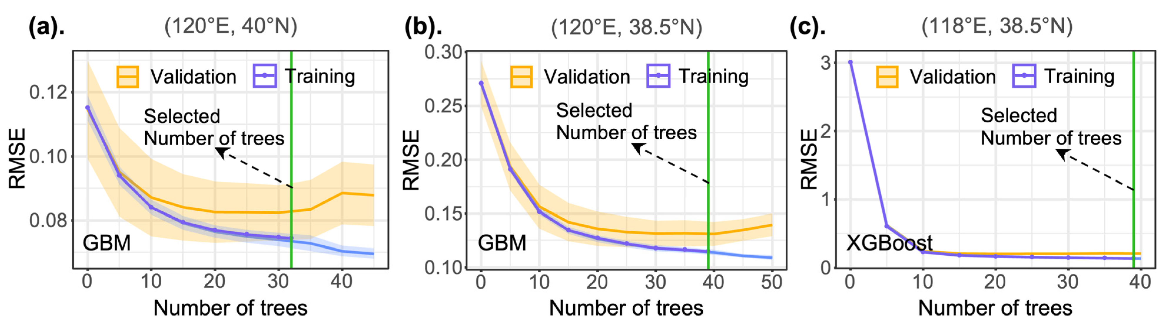
3.3. Model Performance

The RMSE and CCC results for the six models using the 31 study point testing sets are shown in Figure 5a–d. As shown in Figure 5a, for the SWH, it can be seen that the RMSE value of H2O and ForecastHybrid at the 31 coordinate points is better and more balanced, with the overall performance of the 31 coordinate points appearing blue, while Autoarima, ATAforcasting, and Rminer performed relatively poorly in terms of RMSE for the 14th to 31st coordinate points. The maximum RMSE value of 0.26 m appears in the Rminer prediction results in the 23rd coordinate point, and the minimum value of 0.07 m appears in the Autokeras, H2O, and ForecastHybrid prediction results in the 4th coordinate point. As shown in Figure 5b, it can be seen that the CCC coefficients of Rminer at the 31 coordinate points were relatively unstable, and H2O, ATAforcasting, and ForecastHybrid were the most stable. The lowest CCC coefficient value of 0.27 appears in the Autoarima prediction results for the fourth coordinate. Similar to the SWH, as shown in Figure 5c for the MWP, the RMSEs of H2O and ForecastHybrid are all blue for the 31 coordinate points, and the performance was stable. The RMSE maximum value of 0.48 s appears in the Rminer prediction results in the 18th coordinate point. The CCC coefficient of Rminer was unstable, and the minimum value of 0.17 appears in the Autoarima prediction result in the 12th coordinate point. As shown in Figure 5d, the overall performances of H2O, ForecastHybrid, and ATAforcasting were relatively stable. The clustering results show that, for the RMSE, Autokeras, H2O, and ForecastHybrid were clustered into one class, and Rminer, ATAforcasting, and Autoarima were clustered into one class. For CCC, Rminer was a single class, and the other five algorithms were clustered into one class.

The MAPE results of the SWH on the testing set are shown in Table S1, with H2O receiving the best MAPE performance for 30 coordinates and Autokeras being judged best for the 28th coordinate with a margin of 0.001. The MAPE results of the MWP on the testing set are shown in Table S2, with H2O returning the best MAPE performance at all 31 coordinates.

Subsequently, at each coordinate point, we collated the best RMSE value (minimum) and the corresponding algorithm package used, as shown in Figure 5e,f. The size of the circle at each coordinate point represents the RMSE value and the color corresponds to the best model type. In the SWH, the best performing model at all 31 coordinate points was H2O, with the minimum RMSE 0.07 m occurring at the 4th coordinate point and the maximum RMSE 0.11 m at the 23rd coordinate point. Specifically, the GBM (n = 13) and the SE (stacked ensemble model, n = 12) in the H2O were judged to be the best models, followed by XGBoost (n = 5), with DL accounting for only one point (n = 1). Figure 5f shows that the best performing model in the MWP at the 31 coordinate points was again H2O, with the minimum RMSE of 0.15 s occurring at the 7th coordinate point and the maximum RMSE of 0.20 s at the 19th and 27th coordinate points. Specifically, the SE (stacked ensemble model, n = 15) and the GBM (n = 10) in the H2O model still dominated, followed by XGBoost (n = 5), with DL accounting for only one point (n = 1). Overall, H2O dominated in the SWH and MWP, surpassing the other algorithm packages in terms of the best performing RMSE values in all coordinate points. For H2O, SE and GBM returned the best results the most times, followed by XGBoost. These three models are essentially ensemble machine learning models. It is worth noting that, although ForecastHybrid did not achieve the best performance, its performance was behind that of H2O, which consumes fewer computing resources, and ForecastHybrid is also essentially an ensemble machine learning model. The deep learning model did not perform satisfactorily, probably because deep learning is more dependent on large amounts of data and is a data-intensive model. The training dataset in this paper only contained 412 items, and the deep learning model sometimes performs poorly on small- and medium-sized datasets.

There is an absence of variable importance score attributes in stacked ensemble models. Therefore, subsequently, we visualized the importance ranking of the feature variables at the 4th coordinate point (120° E, 40° N), the 23rd coordinate point (120° E, 38.5° N), and the 19th coordinate point (118° E, 38.5° N), as shown in Figure 5g. In the figure, index.num is the trend in a granularity of seconds, month.xts is the number of months aligning the month range from 0 to 11, week4 is the modulus for a four-week frequency, week.iso is the number of weeks in a year that lie under the ISO calendar, and yday is the number of days in a year. The results show that the week, yday, and week.iso features were the most important among the minimum RMSE coordinate points in the SWH. In the SWH maximum RMSE coordinates, the week.iso, week4, and quarter features were the most important. In the MWP maximum coordinates, the week 4, week.iso, and yday features were the most important. In particular, in the SWH minimum RMSE coordinate point (121.5° E, 40° N) and the other maximum RMSE coordinate point (119.5° E, 38° N), the corresponding models are ensemble learning models without the variable importance of data features. Subsequently, we visualize the learning curve on these three coordinate points, as shown in Figure 6. The yellow curve represents the validation set, the purple curve represents the training set, and the shading is the confidence interval. The green vertical bars are the selected hyperparameter values. The choice of optimal hyperparameters is slightly biased, because for H2O-AutoML, setting the stop training strategy can only be set to the longest running time and the maximum number of trained models. Under the first stopping strategy, in order to train as many models of different algorithm types as possible, H2O-AutoML will perform interval sampling within a fixed hyperparameter range, which will lead to more or less deviation from the optimal situation. For the second case, further discussion is still needed. However, both can be mitigated by boosting computing resources and increasing the maximum runtime. In order to avoid overfitting or underfitting, within H2O-AutoML, an inner validation dataset is required to compare the model performance of the same type and different hyperparameters. It can be seen that the errors of three representative coordinates on the training and validation sets gradually converge. Furthermore, close to the turning point where the validation set error begins to increase in reverse, appropriate hyperparameters are selected.

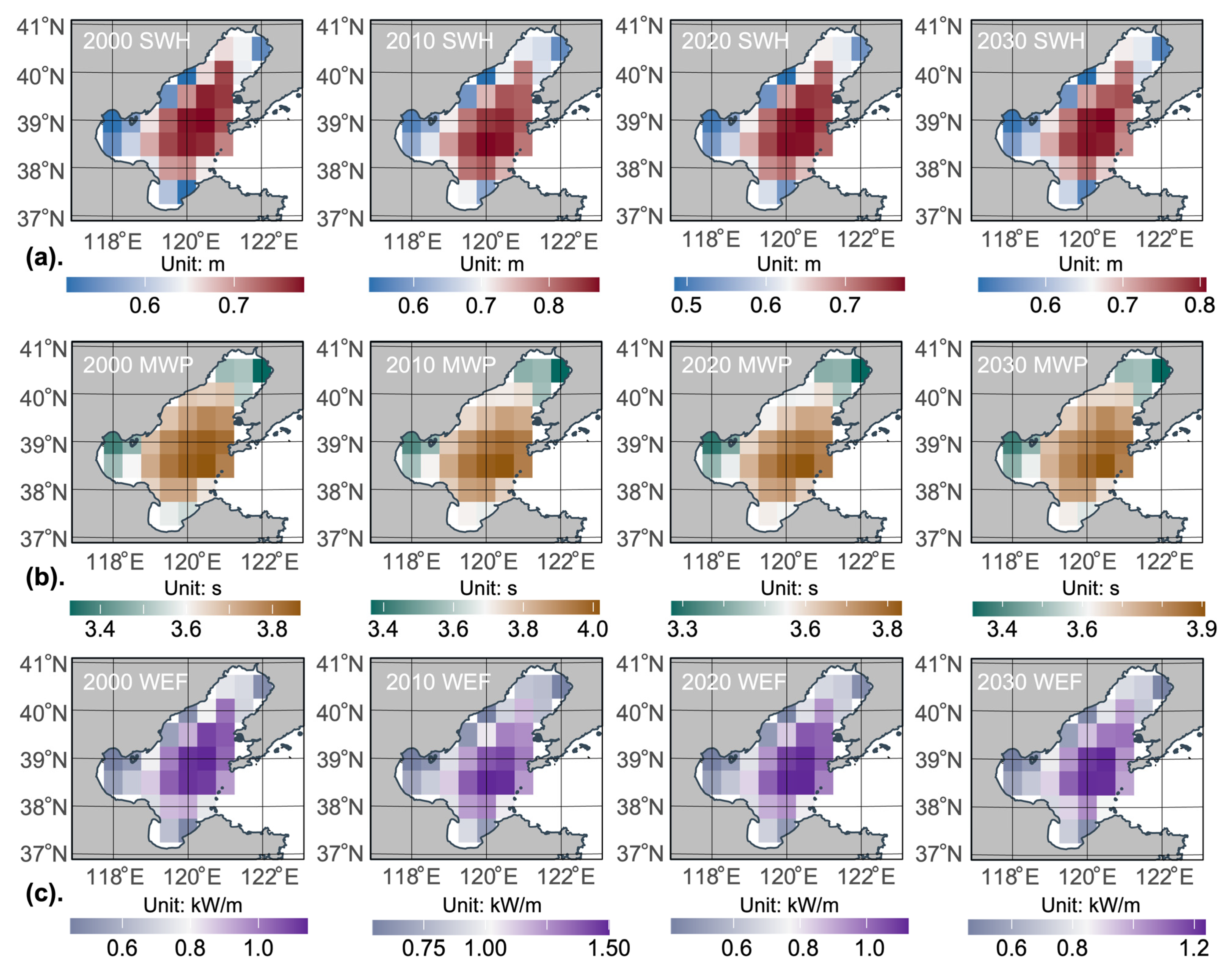
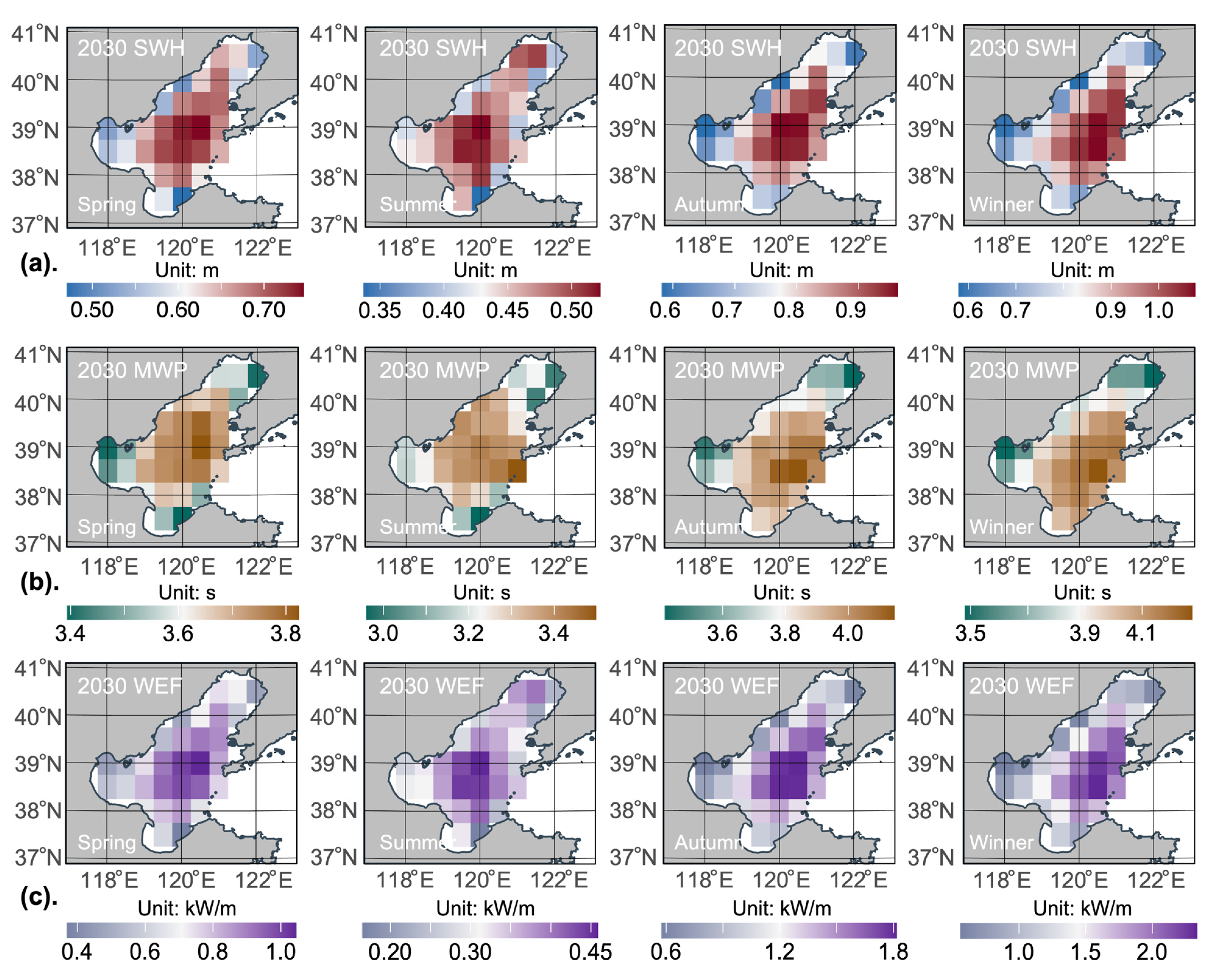
3.4. Wave Energy Flux Prediction

The essence of energy flux prediction is the prediction of the SWH and MWP, and we combined the RMSE and MAPE metrics to select the best model for prediction at each coordinate point. As in Figure 5e,f, the H2O algorithm package was used for all coordinate points. The forecast steps were 108, and the forecast time was up to 2030. The visualization results for the Bohai Sea from 2000 to 2030 with a 10-year cycle are shown in Figure 7. In the past 20 years and in the next 10 years, the SWH, MWP, and the WEF changes remain relatively stable, with different distributions in the middle of the sea and near the ground. Specifically, on the annual average at each coordinate point, the SWH is higher in the central Bohai Sea, with the highest value not exceeding 1 m. Among the three bays in the Bohai Sea, the SWH is the smallest in Bohai Bay (west), probably because it is the farthest from the Bohai Strait (east), which weakens the influence of external currents such as the Yellow Sea (east). Secondly, it may also be related to the water depth. The terrain of the entire Bohai Sea is relatively flat, but from the three directions of Liaodong Bay (north), Bohai Bay, and Laizhou Bay (south), it gradually slopes towards the central shallow basin of the Bohai Sea and the Bohai Strait. For MWP, it is also the largest in the central Bohai Sea and the smallest in Liaodong Bay and Bohai Bay, and the annual average maximum value of each coordinate point does not exceed 4.5 s. For WEF, it is also the largest in the central Bohai Sea, followed by Liaodong Bay, and the annual average maximum value at each coordinate point is around 1.5 kW/m. Bohai Bay is the smallest, followed by Laizhou Bay. The seasonal visualization results of the SWH, MWP, and WEF in 2030 are shown in Figure 8. As shown in Figure 8a, the SWH in the Bohai Sea in 2030 exhibits a distribution trend that is higher in the middle of the sea and smaller in the near-surface area. Due to the alternation of monsoons, the waves in the Bohai Sea have significant seasonality. The SWH in autumn and winter is larger than in spring and summer, which is consistent with the results of previous seasonal analyses. At the same time, compared with spring and summer, in autumn and winter, the difference of SWH between the central sea area and the land is larger, and the minimum value appears in Bohai Bay. The MWP in 2030 shown in Figure 8b is similar to the SWH distribution, with longer periods in the middle of the sea and shorter periods in coastal regions.

The MWP in autumn and winter is also larger than in spring and autumn. The overall trend of the WEF in 2030 shown in Figure 8c is high in the middle and low around the coasts. As compared with other seasons, the energy flux is larger in the autumn and winter periods, which is in accordance with the study of Dunnett et al., regarding wave energy in Canada [97].

The characterization of ocean wave properties will ensure that appropriate techniques are applied to extract the most energy. The lower density flux suggests that emerging energy conversion devices, such as sealed-buoy wave energy converters [98] and triboelectric nanogenerators (TENGs), which are suitable for low-frequency wave motion, would be beneficial for wave energy development in the Bohai Sea. In the laboratory test stage, the wave energy harvesting device should consider the sea conditions of the actual deployment area, such as the sea surface temperature, wave period, significant wave, and other ocean parameters. Especially in the low energy flow density and low sea area of the Bohai Sea, it is particularly important for the construction, operation, and maintenance of energy conversion devices to adapt and optimize the conversion efficiency of the device and consider the changing trend of sea conditions in the future.

4. Conclusions

In this study, we applied automated machine learning to predict the SWH and the MWP in the Bohai Sea to calculate the WEF. To the best of our knowledge, this is the first time that this has been performed. By comparing conventional machine learning with automated machine learning, we found that automated machine learning algorithms with a large number of basic learners have significant advantages. Among the 31 coordinate research points in the Bohai Sea, the H2O automated machine learning algorithm achieved the best performance. The majority of the best models within the H2O algorithm are integrated learning models, such as GBM, XGBoost, and SE. As compared with the real data, the best model prediction results were relatively smooth and stable; however, this did not reflect the full range of outlier states. Moreover, with the same model training resources, the best models for different coordinate points were different, and point-by-point training and prediction can effectively adapt to the spatial variability of the data. The WEF indicates a central regional concentration trend in the Bohai Sea, with less energy in the surrounding near-shore region. At the same time, the annual average values of SWH, MWP, and WEF at each research coordinate point in the Bohai Sea are relatively stable. WEF has low energy density, and the maximum annual average value does not exceed 1.5 kW/m, becoming higher in autumn and winter. The lower wave energy flux density in the Bohai Sea indicates that the use of wave energy conversion devices that capture low frequencies can better adapt to the wave characteristics of the Bohai Sea. In this study, we considered direct factors, such as the MWP and SWH, and did not consider other factors, such as the salinity, temperature, and UV wind. Furthermore, the Kriging method and the inverse distance weighted method can be used to spatially interpolate the data to refine the analysis of an area. At the same time, the reanalysis dataset used has certain limitations for characterizing SWH, MWP, and WEF. In the future, sensor data collected by actual equipment such as buoys can be considered. Although this study focused solely on the Bohai Sea, the automated machine learning method presented in this paper provides new insights into the prediction of ocean parameters. The SWH, MWP, and WEF results obtained from the analysis and prediction provide ocean parameter characterization for the design and deployment of wave energy harvesting devices in low-energy-density sea areas.

References

1. Zou, C.; Xiong, B.; Xue, H.; Zheng, D.; Ge, Z.; Wang, Y.; Jiang, L.; Pan, S.; Wu, S. The Role of New Energy in Carbon Neutral. Pet. Explor. Dev. 2021, 48, 480–491. [Google Scholar] [CrossRef]
2. Smith, A.M.; Brown, M.A. Demand Response: A Carbon-Neutral Resource? Energy 2015, 85, 10–22. [Google Scholar] [CrossRef] [Green Version]
3. Zhao, X.; Ma, X.; Chen, B.; Shang, Y.; Song, M. Challenges toward Carbon Neutrality in China: Strategies and Countermeasures. Resour. Conserv. Recycl. 2022, 176, 105959. [Google Scholar] [CrossRef]
4. Dong, L.; Miao, G.; Wen, W. China’s Carbon Neutrality Policy: Objectives, Impacts and Paths. East Asian Policy 2021, 13, 5–18. [Google Scholar] [CrossRef]
5. Prasad, S.; Venkatramanan, V.; Singh, A. Renewable Energy for a Low-Carbon Future: Policy Perspectives. In Sustainable Bioeconomy: Pathways to Sustainable Development Goals; Venkatramanan, V., Shah, S., Prasad, R., Eds.; Springer: Singapore, 2021; pp. 267–284. ISBN 9789811573217. [Google Scholar]
6. Quereshi, S.; Jadhao, P.R.; Pandey, A.; Ahmad, E.; Pant, K.K. 1—Overview of Sustainable Fuel and Energy Technologies. In Sustainable Fuel Technologies Handbook; Dutta, S., Mustansar Hussain, C., Eds.; Academic Press: Cambridge, MA, USA, 2021; pp. 3–25. ISBN 978-0-12-822989-7. [Google Scholar]
7. Agarwal, U.; Jain, N.; Kumawat, M. Ocean Energy: An Endless Source of Renewable Energy. Available online: https://www.igi-global.com/chapter/ocean-energy/www.igi-global.com/chapter/ocean-energy/293178 (accessed on 10 February 2022).
8. Feng, C.; Ye, G.; Jiang, Q.; Zheng, Y.; Chen, G.; Wu, J.; Feng, X.; Si, Y.; Zeng, J.; Li, P.; et al. The Contribution of Ocean-Based Solutions to Carbon Reduction in China. Sci. Total Environ. 2021, 797, 149168. [Google Scholar] [CrossRef]
9. Zhang, Y.; Zhao, Y.; Sun, W.; Li, J. Ocean Wave Energy Converters: Technical Principle, Device Realization, and Performance Evaluation. Renew. Sustain. Energy Rev. 2021, 141, 110764. [Google Scholar] [CrossRef]
10. Madan, D.; Rathnakumar, P.; Marichamy, S.; Ganesan, P.; Vinothbabu, K.; Stalin, B. A Technological Assessment of the Ocean Wave Energy Converters. In Advances in Industrial Automation and Smart Manufacturing; Arockiarajan, A., Duraiselvam, M., Raju, R., Eds.; Springer: Singapore, 2021; pp. 1057–1072. [Google Scholar]
11. Ahamed, R.; McKee, K.; Howard, I. Advancements of Wave Energy Converters Based on Power Take Off (PTO) Systems: A Review. Ocean Eng. 2020, 204, 107248. [Google Scholar] [CrossRef]
12. Wu, J.; Qin, L.; Chen, N.; Qian, C.; Zheng, S. Investigation on a Spring-Integrated Mechanical Power Take-off System for Wave Energy Conversion Purpose. Energy 2022, 245, 123318. [Google Scholar] [CrossRef]
13. Cai, Q.; Zhu, S. Applying Double-Mass Pendulum Oscillator with Tunable Ultra-Low Frequency in Wave Energy Converters. Appl. Energy 2021, 298, 117228. [Google Scholar] [CrossRef]
14. Li, Q.; Mi, J.; Li, X.; Chen, S.; Jiang, B.; Zuo, L. A Self-Floating Oscillating Surge Wave Energy Converter. Energy 2021, 230, 120668. [Google Scholar] [CrossRef]
15. Falnes, J. A Review of Wave-Energy Extraction. Mar. Struct. 2007, 20, 185–201. [Google Scholar] [CrossRef]
16. Fan, F.-R.; Tian, Z.-Q.; Wang, Z.L. Flexible Triboelectric Generator. Nano Energy 2012, 1, 328–334. [Google Scholar] [CrossRef]
17. Zi, Y.; Guo, H.; Wen, Z.; Yeh, M.-H.; Hu, C.; Wang, Z.L. Harvesting Low-Frequency (<5 Hz) Irregular Mechanical Energy: A Possible Killer Application of Triboelectric Nanogenerator. ACS Nano 2016, 10, 4797–4805. [Google Scholar] [CrossRef]
18. Wang, Z.L. Triboelectric Nanogenerators as New Energy Technology and Self-Powered Sensors—Principles, Problems and Perspectives. Faraday Discuss. 2015, 176, 447–458. [Google Scholar] [CrossRef]
19. Wang, Z.L. Catch Wave Power in Floating Nets. Nature 2017, 542, 159–160. [Google Scholar] [CrossRef]
20. Rodrigues, C.; Nunes, D.; Clemente, D.; Mathias, N.; Correia, J.M.; Rosa-Santos, P.; Taveira-Pinto, F.; Morais, T.; Pereira, A.; Ventura, J. Emerging Triboelectric Nanogenerators for Ocean Wave Energy Harvesting: State of the Art and Future Perspectives. Energy Environ. Sci. 2020, 13, 2657–2683. [Google Scholar] [CrossRef]
21. Dvorak, M.J.; Archer, C.L.; Jacobson, M.Z. California Offshore Wind Energy Potential. Renew. Energy 2010, 35, 1244–1254. [Google Scholar] [CrossRef]
22. Wan, Y.; Fan, C.; Dai, Y.; Li, L.; Sun, W.; Zhou, P.; Qu, X. Assessment of the Joint Development Potential of Wave and Wind Energy in the South China Sea. Energies 2018, 11, 398. [Google Scholar] [CrossRef] [Green Version]
23. Liu, G.; Wu, W.; Ge, Q.; Dai, E.; Wan, Z.; Zhou, Y. GIS-Based Assessment of Roof-Mounted Solar Energy Potential in Jiangsu, China. In Proceedings of the 2011 Second International Conference on Digital Manufacturing Automation, Zhangjiajie, China, 5–7 August 2011; pp. 565–571. [Google Scholar]
24. Dasari, H.P.; Desamsetti, S.; Langodan, S.; Attada, R.; Kunchala, R.K.; Viswanadhapalli, Y.; Knio, O.; Hoteit, I. High-Resolution Assessment of Solar Energy Resources over the Arabian Peninsula. Appl. Energy 2019, 248, 354–371. [Google Scholar] [CrossRef]
25. Odhiambo, M.R.O.; Abbas, A.; Wang, X.; Mutinda, G. Solar Energy Potential in the Yangtze River Delta Region—A GIS-Based Assessment. Energies 2021, 14, 143. [Google Scholar] [CrossRef]
26. Iglesias, G.; López, M.; Carballo, R.; Castro, A.; Fraguela, J.A.; Frigaard, P. Wave Energy Potential in Galicia (NW Spain). Renew. Energy 2009, 34, 2323–2333. [Google Scholar] [CrossRef]
27. Wang, H.; Fu, D.; Liu, D.; Xiao, X.; He, X.; Liu, B. Analysis and Prediction of Significant Wave Height in the Beibu Gulf, South China Sea. J. Geophys. Res. Oceans 2021, 126, e2020JC017144. [Google Scholar] [CrossRef]
28. Sierra, J.P.; Martín, C.; Mösso, C.; Mestres, M.; Jebbad, R. Wave Energy Potential along the Atlantic Coast of Morocco. Renew. Energy 2016, 96, 20–32. [Google Scholar] [CrossRef]
29. Zhou, D.; Yu, M.; Yu, J.; Li, Y.; Guan, B.; Wang, X.; Wang, Z.; Lv, Z.; Qu, F.; Yang, J. Impacts of Inland Pollution Input on Coastal Water Quality of the Bohai Sea. Sci. Total Environ. 2021, 765, 142691. [Google Scholar] [CrossRef]
30. Alpaydin, E. Introduction to Machine Learning; MIT Press: Cambridge, MA, USA, 2020; ISBN 0-262-04379-3. [Google Scholar]
31. Wright, R.E. Logistic Regression; American Psychological Association: Washington, DC, USA, 1995. [Google Scholar]
32. Hearst, M.A.; Dumais, S.T.; Osuna, E.; Platt, J.; Scholkopf, B. Support Vector Machines. IEEE Intell. Syst. Appl. 1998, 13, 18–28. [Google Scholar] [CrossRef] [Green Version]
33. Chen, T.; He, T.; Benesty, M.; Khotilovich, V.; Tang, Y.; Cho, H.; Chen, K. Extreme Gradient Boosting [R Package xgboost Version 1.6.0.1]. 2022. Available online: https://cran.r-project.org/web/packages/xgboost/index.html (accessed on 23 May 2022).
34. Liu, M.; Huang, Y.; Li, Z.; Tong, B.; Liu, Z.; Sun, M.; Jiang, F.; Zhang, H. The Applicability of LSTM-KNN Model for Real-Time Flood Forecasting in Different Climate Zones in China. Water 2020, 12, 440. [Google Scholar] [CrossRef] [Green Version]
35. Jamil, S.; Rahman, M.; Haider, A. Bag of Features (BoF) Based Deep Learning Framework for Bleached Corals Detection. Big Data Cogn. Comput. 2021, 5, 53. [Google Scholar] [CrossRef]
36. Sun, M.; Li, Z.; Yao, C.; Liu, Z.; Wang, J.; Hou, A.; Zhang, K.; Huo, W.; Liu, M. Evaluation of Flood Prediction Capability of the WRF-Hydro Model Based on Multiple Forcing Scenarios. Water 2020, 12, 874. [Google Scholar] [CrossRef] [Green Version]
37. Yao, X. Evolving Artificial Neural Networks. Proc. IEEE 1999, 87, 1423–1447. [Google Scholar]
38. McCulloch, W.S.; Pitts, W. A Logical Calculus of the Ideas Immanent in Nervous Activity. Bull. Math. Biophys. 1943, 5, 115–133. [Google Scholar] [CrossRef]
39. Medsker, L.R.; Jain, L.C. Recurrent Neural Networks. Des. Appl. 2001, 5, 64–67. [Google Scholar]
40. O’Shea, K.; Nash, R. An Introduction to Convolutional Neural Networks. arXiv 2015, arXiv:1511.08458. [Google Scholar]
41. Valueva, M.V.; Nagornov, N.N.; Lyakhov, P.A.; Valuev, G.V.; Chervyakov, N.I. Application of the Residue Number System to Reduce Hardware Costs of the Convolutional Neural Network Implementation. Math. Comput. Simul. 2020, 177, 232–243. [Google Scholar] [CrossRef]
42. Hochreiter, S.; Schmidhuber, J. Long Short-Term Memory. Neural Comput. 1997, 9, 1735–1780. [Google Scholar] [CrossRef]
43. He, K.; Zhang, X.; Ren, S.; Sun, J. Deep Residual Learning for Image Recognition. In Proceedings of the IEEE Conference on Computer Vision and Pattern Recognition, Las Vegas, NV, USA, 27–30 June 2016; pp. 770–778. [Google Scholar]
44. Abdel-Aal, R.E.; Elhadidy, M.A.; Shaahid, S.M. Modeling and Forecasting the Mean Hourly Wind Speed Time Series Using GMDH-Based Abductive Networks. Renew. Energy 2009, 34, 1686–1699. [Google Scholar] [CrossRef]
45. Jamil, S.; Abbas, M.S.; Roy, A.M. Distinguishing Malicious Drones Using Vision Transformer. AI 2022, 3, 260–273. [Google Scholar] [CrossRef]
46. Sun, A.Y.; Scanlon, B.R.; Save, H.; Rateb, A. Reconstruction of GRACE Total Water Storage Through Automated Machine Learning. Water Resour. Res. 2021, 57, e2020WR028666. [Google Scholar] [CrossRef]
47. Bergstra, J.; Bengio, Y. Random Search for Hyper-Parameter Optimization. J. Mach. Learn. Res. 2012, 13, 281–305. [Google Scholar]
48. Bao, Y.; Liu, Z. A Fast Grid Search Method in Support Vector Regression Forecasting Time Series. In Proceedings of the Intelligent Data Engineering and Automated Learning—IDEAL 2006, Burgos, Spain, 20–23 September 2006; Corchado, E., Yin, H., Botti, V., Fyfe, C., Eds.; Springer: Berlin/Heidelberg, Germany, 2006; pp. 504–511. [Google Scholar]
49. Brochu, E.; Cora, V.M.; de Freitas, N. A Tutorial on Bayesian Optimization of Expensive Cost Functions, with Application to Active User Modeling and Hierarchical Reinforcement Learning. arXiv 2010, arXiv:1012.2599. [Google Scholar]
50. Koh, J.C.O.; Spangenberg, G.; Kant, S. Automated Machine Learning for High-Throughput Image-Based Plant Phenotyping. Remote Sens. 2021, 13, 858. [Google Scholar] [CrossRef]
51. Han, T.; Gois, F.N.B.; Oliveira, R.; Prates, L.R.; Porto, M.M.D.A. Modeling the Progression of COVID-19 Deaths Using Kalman Filter and AutoML. Soft Comput. 2021. [Google Scholar] [CrossRef]
52. Liu, X.; Taylor, M.P.; Aelion, C.M.; Dong, C. Novel Application of Machine Learning Algorithms and Model-Agnostic Methods to Identify Factors Influencing Childhood Blood Lead Levels. Environ. Sci. Technol. 2021, 55, 13387–13399. [Google Scholar] [CrossRef]
53. Hersbach, H.; Bell, B.; Berrisford, P.; Hirahara, S.; Horanyi, A.; Muñoz-Sabater, J.; Nicolas, J.; Peubey, C.; Radu, R.; Schepers, D.; et al. The ERA5 Global Reanalysis. Q. J. R. Meteorol. Soc. 2020, 146, 1999–2049. [Google Scholar] [CrossRef]
54. Hersbach, H.; Bell, B.; Berrisford, P.; Biavati, G.; Horányi, A.; Muñoz Sabater, J.; Nicolas, J.; Peubey, C.; Radu, R.; Rozum, I.; et al. ERA5 Monthly Averaged Data on Single Levels from 1979 to Present. Copernic. Clim. Change Serv. C3S Clim. Data Store CDS 2019, 10, 252–266. [Google Scholar] [CrossRef]
55. Wang, J.; Li, B.; Gao, Z.; Wang, J. Comparison of ECMWF Significant Wave Height Forecasts in the China Sea with Buoy Data. Weather Forecast. 2019, 34, 1693–1704. [Google Scholar] [CrossRef]
56. Wang, J.; Wang, Y. Evaluation of the ERA5 Significant Wave Height against NDBC Buoy Data from 1979 to 2019. Mar. Geod. 2022, 45, 151–165. [Google Scholar] [CrossRef]
57. Wang, J.; Liu, J.; Wang, Y.; Liao, Z.; Sun, P. Spatiotemporal Variations and Extreme Value Analysis of Significant Wave Height in the South China Sea Based on 71-Year Long ERA5 Wave Reanalysis. Appl. Ocean Res. 2021, 113, 102750. [Google Scholar] [CrossRef]
58. Mahmoodi, K.; Ghassemi, H.; Razminia, A. Temporal and Spatial Characteristics of Wave Energy in the Persian Gulf Based on the ERA5 Reanalysis Dataset. Energy 2019, 187, 115991. [Google Scholar] [CrossRef]
59. Mayer, L.; Jakobsson, M.; Allen, G.; Dorschel, B.; Falconer, R.; Ferrini, V.; Lamarche, G.; Snaith, H.; Weatherall, P. The Nip-pon Foundation—GEBCO Seabed 2030 Project: The Quest to See the World’s Oceans Completely Mapped by 2030. Geosciences 2018, 8, 63. [Google Scholar] [CrossRef] [Green Version]
60. Weatherall, P.; Tozer, B.; Arndt, J.E.; Bazhenova, E.; Bringensparr, C.; Castro, C.; Dorschel, B.; Drennon, H.; Ferrini, V.; Harper, H.; et al. The GEBCO_2021 Grid—A Continuous Terrain Model of the Global Oceans and Land; NERC EDS British Oceanographic Data Centre NOC: Liverpool, UK, 2021. [Google Scholar] [CrossRef]
61. Hashim, M.; Nayan, N.; Setyowati, D.L.; Said, Z.M.; Mahat, H.; Saleh, Y. Analysis of Water Quality Trends Using the Mann-Kendall Test and Sen’s Estimator of Slope in a Tropical River Basin. Pollution 2021, 7, 933–942. [Google Scholar] [CrossRef]
62. Mann, H.B. Nonparametric Tests against Trend. Econometrica 1945, 13, 245–259. [Google Scholar] [CrossRef]
63. Kendall, M.G. Rank Correlation Methods, 2nd ed.; Hafner Publishing Co.: Oxford, UK, 1955; pp. 7–196. [Google Scholar]
64. Iacobucci, D.; Posavac, S.S.; Kardes, F.R.; Schneider, M.J.; Popovich, D. The Median Split: Robust, Refined, and Revived. J. Consum. Psychol. 2015, 25, 690–704. [Google Scholar] [CrossRef]
65. Yapar, G.; Selamlar, H.T.; Capar, S.; Yavuz, İ. ATA Method. Hacet. J. Math. Stat. 2019, 48, 1838–1844. [Google Scholar] [CrossRef]
66. Yapar, G. Modified Simple Exponential Smoothing. Hacet. J. Math. Stat. 2018, 47, 741–754. [Google Scholar] [CrossRef]
67. Yapar, G.; Capar, S.; Selamlar, H.T.; Yavuz, İ. Modified Holt’s Linear Trend Method. Hacet. J. Math. Stat. 2018, 47, 1394–1403. [Google Scholar]
68. Taylan, A.S.; Selamlar, H.T.; Yapar, G. ATAforecasting: Automatic Time Series Analysis and Forecasting Using the Ata Method. R J. 2021, 13, 507–541. [Google Scholar] [CrossRef]
69. Shaub, D.; Ellis, P. Convenient Functions for Ensemble Time Series Forecasts [R Package forecastHybrid Version 5.0.19]. 2022. Available online: https://cran.r-project.org/web/packages/forecastHybrid/index.html (accessed on 25 May 2022).
70. Panigrahi, S.; Behera, H.S. A Hybrid ETS–ANN Model for Time Series Forecasting. Eng. Appl. Artif. Intell. 2017, 66, 49–59. [Google Scholar] [CrossRef]
71. Shaub, D. Fast and Accurate Yearly Time Series Forecasting with Forecast Combinations. Int. J. Forecast. 2020, 36, 116–120. [Google Scholar] [CrossRef]
72. Brożyna, J.; Mentel, G.; Szetela, B.; Strielkowski, W. Multi-Seasonality in the TBATS Model Using Demand for Electric Energy as a Case Study. Econ. Comput. Econ. Cybern. Stud. Res. 2018, 52, 229–246. [Google Scholar] [CrossRef]
73. Zhang, H. The Optimality of Naive Bayes. Aa 2004, 1, 3. [Google Scholar]
74. Hyndman, R.; Athanasopoulos, G.; Bergmeir, C.; Caceres, G.; Chhay, L.; O’Hara-Wild, M.; Petropoulos, F.; Razbash, S.; Wang, E.; Yasmeen, F.; et al. Forecasting Functions for Time Series and Linear Models [R Package Forecast Version 8.17.0]. 2022. Available online: https://cran.r-project.org/web/packages/forecast/index.html (accessed on 29 May 2022).
75. Hyndman, R.J.; Khandakar, Y. Automatic Time Series Forecasting: The Forecast Package for R. J. Stat. Softw. 2008, 27, 1–22. [Google Scholar] [CrossRef] [Green Version]
76. Hillmer, S.C.; Tiao, G.C. An ARIMA-Model-Based Approach to Seasonal Adjustment. J. Am. Stat. Assoc. 1982, 77, 63–70. [Google Scholar] [CrossRef]
77. LeDell, E.; Poirier, S. H2O Automl: Scalable Automatic Machine Learning. In Proceedings of the AutoML Workshop at ICML, Vienna, Austria, 18 July 2020; Volume 2020. [Google Scholar]
78. Nelder, J.A.; Wedderburn, R.W. Generalized Linear Models. J. R. Stat. Soc. Ser. A 1972, 135, 370–384. [Google Scholar] [CrossRef]
79. Svozil, D.; Kvasnicka, V.; Pospichal, J. Introduction to Multi-Layer Feed-Forward Neural Networks. Chemom. Intell. Lab. Syst. 1997, 39, 43–62. [Google Scholar] [CrossRef]
80. Friedman, J.H. Greedy Function Approximation: A Gradient Boosting Machine. Ann. Statist. 2001, 29, 1189–1232. [Google Scholar] [CrossRef]
81. Chen, T.; Guestrin, C. XGBoost: A Scalable Tree Boosting System. In Proceedings of the KDD’16: The 22nd ACM SIGKDD International Conference on Knowledge Discovery and Data Mining, San Francisco, CA, USA, 13–17 August 2016; Association for Computing Machinery: New York, NY, USA, 2016; pp. 785–794. [Google Scholar] [CrossRef] [Green Version]
82. Geurts, P.; Ernst, D.; Wehenkel, L. Extremely Randomized Trees. Mach. Learn. 2006, 63, 3–42. [Google Scholar] [CrossRef] [Green Version]
83. Wolpert, D.H. Stacked Generalization. Neural Netw. 1992, 5, 241–259. [Google Scholar] [CrossRef]
84. Van Der Laan, M.J.; Polley, E.C.; Hubbard, A.E. Super Learner. Stat. Appl. Genet. Mol. Biol. 2007, 6, 25. [Google Scholar] [CrossRef]
85. Cortez, P. Data Mining with Neural Networks and Support Vector Machines Using the R/Rminer Tool. In Proceedings of the Advances in Data Mining. Applications and Theoretical Aspects, New York, NY, USA, 16–21 July 2013; Perner, P., Ed.; Springer: Berlin/Heidelberg, Germany, 2010; pp. 572–583. [Google Scholar]
86. Cortez, P. Data Mining Classification and Regression Methods [R Package rminer Version 1.4.6]. 2022. Available online: https://cran.r-project.org/web/packages/rminer/index.html (accessed on 30 May 2022).
87. Keerthi, S.S.; Lin, C.-J. Asymptotic Behaviors of Support Vector Machines with Gaussian Kernel. Neural Comput. 2003, 15, 1667–1689. [Google Scholar] [CrossRef]
88. Breiman, L. Random Forests. Mach. Learn. 2001, 45, 5–32. [Google Scholar] [CrossRef] [Green Version]
89. Dey, R.; Salem, F.M. Gate-Variants of Gated Recurrent Unit (GRU) Neural Networks. In Proceedings of the 2017 IEEE 60th International Midwest Symposium on Circuits and Systems (MWSCAS), Boston, MA, USA, 6–9 August 2017; pp. 1597–1600. [Google Scholar]
90. Liang, B.; Shao, Z.; Wu, G.; Shao, M.; Sun, J. New Equations of Wave Energy Assessment Accounting for the Water Depth. Appl. Energy 2017, 188, 130–139. [Google Scholar] [CrossRef]
91. Beji, S. Improved Explicit Approximation of Linear Dispersion Relationship for Gravity Waves. Coast. Eng. 2013, 73, 11–12. [Google Scholar] [CrossRef]
92. Simarro, G.; Orfila, A. Improved Explicit Approximation of Linear Dispersion Relationship for Gravity Waves: Another Discussion. Coast. Eng. 2013, 80, 15. [Google Scholar] [CrossRef]
93. Cornett, A.M. A Global Wave Energy Resource Assessment. In Proceedings of the Eighteenth International Offshore and Polar Engineering Conference, Vancouver, BC, Canada, 6–17 July 2008. [Google Scholar]
94. Amante, C.; Eakins, B.W. Eakins ETOPO1 1 Arc-Minute Global Relief Model: Procedures, Data Sources and Analysis; Technical Memorandum NESDIS NGDC-24; National Geophysical Data Center, NOAA: Boulder, CO, USA, 2009. [CrossRef]
95. Vihtakari, M. Plot Data on Oceanographic Maps using ‘ggplot2’ [R Package ggOceanMaps Version 1.2.6]. 2022. Available online: https://cran.r-project.org/web/packages/ggOceanMaps/index.html (accessed on 30 May 2022).
96. Shi, J.; Zheng, J.; Zhang, C.; Joly, A.; Zhang, W.; Xu, P.; Sui, T.; Chen, T. A 39-Year High Resolution Wave Hindcast for the Chinese Coast: Model Validation and Wave Climate Analysis. Ocean Eng. 2019, 183, 224–235. [Google Scholar] [CrossRef]
97. Dunnett, D.; Wallace, J.S. Electricity Generation from Wave Power in Canada. Renew. Energy 2009, 34, 179–195. [Google Scholar] [CrossRef]
98. Chen, F.; Duan, D.; Han, Q.; Yang, X.; Zhao, F. Study on Force and Wave Energy Conversion Efficiency of Buoys in Low Wave Energy Density Seas. Energy Convers. Manag. 2019, 182, 191–200. [Google Scholar] [CrossRef]
Figure 1. Summary of research, including data processing, statistical analysis, and modeling procedures.
Jmse 10 01025 g001
Figure 2. H2O-AutoML workflow.
Jmse 10 01025 g002
Figure 3. Annual averages of significant wave height (a) and mean wave period (b) in 2021, both globally and in the study area, with 31 research coordinates in the Bohai Sea (c).
Jmse 10 01025 g003
Figure 4. Correlation analysis (a), seasonal trend analysis (b,c), linear regression (d,e), and Mann–Kendall trend testing (f,g) for the MWP and SWH.
Jmse 10 01025 g004
Figure 5. Performance results of the testing set for the six algorithm packages at 31 study coordinate points: RMSE (a) and CCC (b) of the SWH; RMSE (c) and CCC (d) of the MWP; minimum RMSE value of the SWH and corresponding algorithm package (e); minimum RMSE value of the MWP and corresponding algorithm package (f); and feature importance score at the three specific points (g).
Jmse 10 01025 g005
Figure 6. H2O-AutoML learning curve at 4th (a), 23rd (b) and 19th (c) coordinate point.
Jmse 10 01025 g006
Figure 7. Mean significant wave height (a), mean wave period (b), and wave energy flux (c) in the Bohai Sea in 2000, 2010, 2020, and 2030.
Jmse 10 01025 g007
Figure 8. Seasonality of significant wave height (a), mean wave period (b), and wave energy flux (c) in the Bohai Sea in 2030, from left to right, in spring, summer, autumn, and winter.
Jmse 10 01025 g008