Multi-AUV Cooperative Navigation Algorithm Based on Temporal Difference Method

Abstract

To reduce the cooperative positioning error and improve the navigation accuracy, a single master–slave AUV cooperative navigation method is proposed in this paper, which mainly focuses on planning the optimal path of the master AUV by the time difference (TD) method, under the premise that the path of the slave AUV has been planned. First, the model of multi-AUV cooperative navigation is established, and the observable problem of the system is analyzed. Second, for the single master–slave AUV cooperative navigation system, a Markov decision process (MDP)-based multi-AUV cooperative navigation model is established, and the master AUV path planning method is designed based on the TD method. Finally, the extended Kalman filter (EKF) and unscented Kalman filter (UKF) nonlinear filtering algorithms are applied to simulate and verify the algorithm that is proposed in this paper. The results show that the theoretical positioning error of the slave AUV can be controlled to about 3.2m by planning the path of the master AUV using the TD method. This method can not only reduce the observation error and positioning error of the slave AUV during the whole cooperative navigation process, but also keep the relative measurement distance between the master AUV and the slave AUV within an appropriate range.

1. Introduction

Autonomous underwater vehicles (AUVs) can move underwater autonomously; they have a sensing capability and are powerful tools for humans to explore and make developments in the ocean [1,2]. The distance, accuracy, and reliability of acoustic detection are greatly affected by the complexity of the underwater environment. A single AUV independent detection operation can no longer meet the current demand. Therefore, a multi-AUV cooperative system was born, which has outstanding advantages such as low cost, high efficiency, fault tolerance, and reconfigurability.

Since the concept of a multi-AUV cooperative system was proposed in the 1980s, the US, UK, Japan, EU, and China have established special research institutes in this field [3,4,5]. The exploration of multi-AUV cooperation and execution in the unknown and challenging ocean environment has attracted tens of thousands of scientists and researchers.

For multi-AUV systems, the basis for performing the task is the ability to navigate and locate accurately. The master–slave system is one of the most commonly used systems. To reduce the cost with improved accuracy, a master–slave multi-AUV cooperative navigation system is proposed. The system consists of multiple slave AUVs and a single master AUV, where the master AUV carries high-precision navigation equipment and provides positioning services to the slave AUVs carrying low-precision navigation equipment. They communicate with each other using acoustic equipment to compensate, to some extent, for the temporary data support when one AUV is not positioned correctly and loses its navigation capability. The slave AUVs correct the navigation errors that are introduced by their dead reckoning (DR) by receiving navigation information.

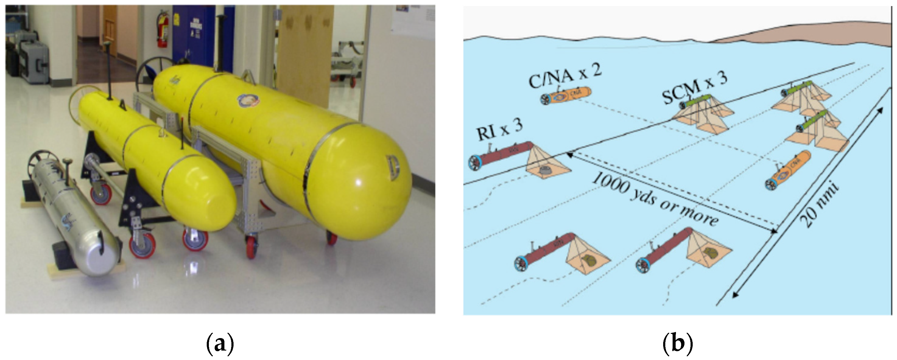
The formation configurations of multi-AUV cooperative navigation can be generally divided into parallel formation and master–slave formation. The European “GREX” project [6,7], the New Jersey Shelf Observation System (NJSS) [8,9], and the MIT-sponsored “CADRE” system [10,11] are typical master–slave cooperative navigation systems. As shown in Figure 1, the CADRE system is a typical master–slave cooperative navigation system, in which the master AUVs are Bluefin-21 and ASV-based communication navigation AUVs, and the slave AUVs are Bluefin-9- and Bluefin-12-based operational AUVs. The system is responsible for searching and mapping, acquisition identification, and other tasks. The system was completed in 2004 for on-lake experiments and has achieved good results in practical applications.

The main goal of cooperative navigation is to suppress error growth and improve positioning accuracy [12]. The cooperative navigation system is a typical nonlinear system, and the standard Kalman filter cannot be applied directly for navigation calculations. The extended Kalman filter (EKF), which linearizes the nonlinear state and measurement equations and then solves them using the standard Kalman filter, is widely used in nonlinear systems [13].

Cao et al. [14] proposed an integrated approach combining biological inspired neurodynamics model (BINM) and velocity synthesis (vs.) methods to solve the cooperative multi-AUV search problem in dynamic underwater environments with ocean currents. The method effectively solves the problem of difficult AUV search targets and longer search paths in the presence of ocean currents.

Song et al. [15] proposed a flow-aided cooperative navigation (FACON) strategy to improve the problem of multiple AUVs failing to surface frequently during actual operations. The method uses marginalized particle filters to track the AUV position, velocity, sensor bias, and unresolved local flow perturbations in ocean forecasts. Simulation experimental results show that asynchronous information fusion among AUVs is achieved by covariance intersection within cooperative AUVs.

Gao et al. [16] proposed a cooperative multi-AUV localization algorithm based on a distributed extended information filter (DEIF) to solve the cooperation problem in decentralized architectures. This approach only requires smaller data transmission packets to effectively solve the communication constrained problem underwater. Simulation and field experimental data show that the algorithm has strong robustness and effectiveness.

Huanget et al. [17] verified the reliability of the proposed adaptive extended Kalman filter method in solving the unknown noise covariance matrix problem in autonomous underwater vehicle colocation through experiments. To minimize the negative effects of outliers that are present in water acoustic communication systems, Li et al. [18] proposed a robust multi-AUV cooperative navigation algorithm based on a Student’s extended Kalman filter (SEKF). Xu et al. [19] improved their previously proposed Huber-based robust algorithm by additionally using adaptive noise estimation for colocalization to achieve a real-time online estimation of the noise statistical properties of the system, and then adaptively adjusting the filtering gain matrix to improve performance. Fan et al. [20] proposed a new robust particle filter based on the maximum correntropy criterion (MCC), which has better robustness, while ensuring estimation accuracy. It is also more efficient and less computationally complex than the existing robust particle filters.

To reduce the cooperative positioning error and improve the navigation accuracy, a single master–slave multi-AUV cooperative navigation system is proposed in this paper. When the path of the slave AUV is determined, planning the path of the master AUV can substantially reduce the observation error of the system. First, an AUV kinematic model was developed to analyze the observability of the master–slave multi-AUV cooperative navigation system and the effect of the observability size on the navigation system. Second, the navigation model under the Markov decision process (MDP) was established. Then, a master AUV path planning method was proposed based on the time difference (TD) method to adapt the path of the slave AUVs. Finally, the simulation was validated by combining the nonlinear filtering method that is commonly used in cooperative navigation, and the superiority of this method over traditional manual path planning was determined and analyzed.

The outline of this article is as follows. Section 2 describes the model and establishes the AUV kinematics equations. Section 3 expounds on the cooperative navigation algorithm based on a single master–slave AUV system. Section 4 analyzes the simulation results of cooperative navigation. Section 5 summarizes the work.

2. Problem Definition

The basis of the AUV cluster operation is to allow for information interaction among several points of AUVs, but the communication problem is one of the bottlenecks that limits the development of AUVs [21]. In a multi-AUV cooperative navigation system, the AUVs share information for cooperative navigation through mutual communication to improve the underwater navigation accuracy of the AUVs [22].

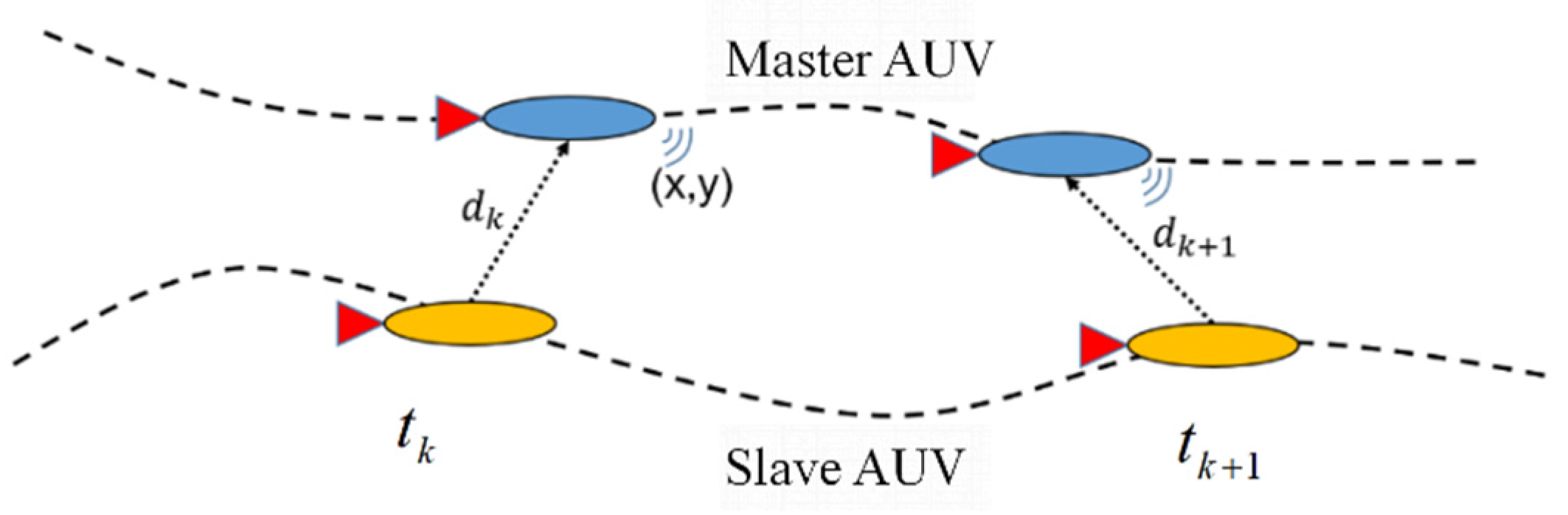
Usually, the master AUV carries high-precision and high-cost navigation equipment; the slave AUV carries low-accuracy and low-cost navigation equipment; and the master and slave AUVs communicate with each other to share information through devices such as acoustic modems. As shown in Figure 2, taking the master–slave structure as an example, the AUVs communicate with each other every ∆t. First, the relative distance and azimuth between the AUVs are measured by the USBL. Next, the master–slave AUVs acquire data on the relative position and attitude angle between them through acoustic devices, and the slave AUVs perform their heading projection using the received data, which is applied to correct the accumulated error of dead reckoning (DR) [23].

2.1. Mathematical Model

First, the motion model of a single AUV was established. Take the eastward position x, northward position y, and heading angle $\psi$ of the AUV as the state vector of the system and neglect the disturbance factors such as ocean currents to establish the following kinematic equations of the AUV [24,25,26].

$$\{\begin{array}{c}{x}_{k+1}=x_k+T{V}_k\cos {\psi }_k\\ y_{k+1}=y_k+T{V}_k\sin {\psi }_k\\ {\psi }_{k+1}={\psi }_k+T{\omega }_k\end{array}$$

(1)

where, at time k + 1, $x_{k+1}$ and $y_{k+1}$ are the position coordinates of the AUV; ${\psi }_{k+1}$ is the yaw angle; and $V_k$ and ${\omega }_k$ are the navigation speed and yaw angle speed, respectively. T is the sampling period.

Equation (1) can be simplified to:

$${\mathit{X}}_{k+1}=\mathit{f}({\mathit{X}}_k,u_k)=\mathit{f}({\mathit{X}}_k,u_{k,m},w_k)={\mathit{X}}_k+{\Psi }_k(u_{k,m}+w_k)$$

(2)

where ${\mathit{X}}_{k+1}={\left[\begin{array}{ccc}{x}_{k+1}& y_{k+1}& {\mathit{\psi }}_{k+1}\end{array}\right]}^T$ is the state of the AUV at time k + 1, u_k denotes the sensor input, ${\mathbf{u}}_k={\mathbf{u}}_{k,m}+{\mathbf{w}}_k$, u_k,m denotes the input that is measured by the sensor, and w_k is the process noise of the system.

${\Psi }_k=\left[\begin{array}{cc}T\cos ({\psi }_k)& 0\\ T\sin ({\psi }_k)& 0\\ 0& T\end{array}\right]$ is the nonlinear term in the model.

Let $\mathit{Q}$ be the system noise covariance matrix; then, we have

$${\mathit{Q}}_k=E\left\{w_k{w}_k^T\right\}=\left[\begin{array}{cc}{\sigma }_{V,k}^2& 0\\ 0& {\sigma }_{\psi ,k}^2\end{array}\right]$$

(3)

For a single master–slave AUV system, ignoring the depth information yields a two-dimensional system with the quantity measured as the distance between AUVs, i.e.,

$$d_{k+1}=\sqrt{(x_{k+1}^s-x_{k+1}^m)+(y_{k+1}^s-y_{k+1}^m)}+{\sigma }_{d,k+1}^{}$$

(4)

where $x_{k+1}^s$ and $y_{k+1}^s$ are the coordinates of the position of the slave AUV at time k + 1, $x_{k+1}^m$ and $y_{k+1}^m$ are the coordinates of the position of the master AUV at time k + 1, and ${\sigma }_{d,k+1}^{}$ is the distance measurement error of the acoustic water measurement equipment.

Converting the above equation into matrix form yields following the measurement equation:

$$Z_{k+1}=h(X_{k+1})+v_{k+1}$$

(5)

where $h(X_{k+1})$ is a nonlinear function with respect to $X_{k+1}$, $v_{k+1}$ denotes the measurement noise matrix.

Let R be the covariance array of the measurement noise of the system; then, we have

$$R_{k+1}=E\left\{v_{k+1}{v}_{k+1}^T\right\}=\left[\begin{array}{c}{\sigma }_{d,k+1}^2\end{array}\right]$$

(6)

The mathematical model of multi-AUV cooperative navigation was established by the above analysis, which provides the theoretical basis for the subsequent analysis.

2.2. Observability Analysis

By definition, a system is observable if the output can fully reflect the properties of the system state [27,28]. Next, the rank criterion is used to analyze the observability of the system.

By ignoring the noise, the state matrix of the system can be written as

$$\{\begin{array}{l}X(k+1)=\mathsf{\Phi }(k+1,k)X(k)\hfill \\ Z(k+1)=H(k+1)X(k+1)\hfill \end{array}$$

(7)

where Z(k + 1) is the observation vector and H(k + 1) is the observation matrix.

According to the rank criterion for linear discrete systems, a sufficient necessary condition for the above system to be fully observable is that its observable discriminant matrix $\mathrm{\Gamma }$ is of full rank, i.e.,

$$\mathrm{rank}\mathrm{\Gamma }=\mathrm{rank}{\left[\begin{array}{cc}\begin{array}{cc}\begin{array}{cc}\mathrm{H}& \mathrm{H}\mathsf{\Phi }\end{array}& \dots \end{array}& \mathrm{H}{\mathsf{\Phi }}^{\mathrm{n}-1}\end{array}\right]}^T=\mathrm{n}$$

(8)

where n is the number of dimensions of the system state vector.

The first-order partial derivatives of the resulting measurement equations from Equation (4) are linearized as follows:

$$H_{k+1}={\frac{\partial h(x)}{\partial x}|}_{x=x_{k+1}}=\left[\begin{array}{cc}\frac{x_{k+1}^s-x_{k+1}^m}{d_{k+1}}& \frac{y_{k+1}^s-y_{k+1}^m}{d_{k+1}}\end{array}\right]$$

(9)

For the two adjacent acoustic measurements, there are

$$\mathrm{\Gamma }(k,k+1)=\left[\begin{array}{c}H(k+1)\\ H(k)\mathsf{\Phi }(k,k)\end{array}\right]=\left[\begin{array}{cc}\frac{x_k^s-x_k^m}{d_k}& \frac{y_k^s-y_k^m}{d_k}\\ \frac{x_{k+1}^s-x_{k+1}^m}{d_{k+1}}& \frac{y_{k+1}^s-y_{k+1}^m}{d_{k+1}}\end{array}\right]$$

(10)

where $\mathsf{\Phi }(k,k)=\left[\begin{array}{cc}1& 0\\ 0& 1\end{array}\right]$.

From Equation (8), it is clear that $\det \mathrm{\Gamma }(k,k+1)\ne 0$. That is, when the determinant of the observable discriminant matrix of the system is not zero, $\mathrm{rank}\mathrm{\Gamma }=2$, and the system is observable.

Now considering the condition that the system is unobservable, let $\det \mathrm{\Gamma }(k,k+1)=0$; then, we have

$$(x_{k+1}^s-x_{k+1}^m)(y_k^s-y_k^m)-(x_k^s-x_k^m)(y_{k+1}^s-y_{k+1}^m)=0$$

(11)

It is obvious that the system is unobservable when two adjacent observations satisfy $\{\begin{array}{l}{x}_{k+1}^s-x_{k+1}^m=0\hfill \\ x_k^s-x_k^m=0\hfill \end{array}$ or $\{\begin{array}{l}{y}_{k+1}^s-y_{k+1}^m=0\hfill \\ y_k^s-y_k^m=0\hfill \end{array}$. That is, the system is observable as long as the observation vector of two adjacent distance measurements $R_{k+1}\ne R_k$.

As shown in Figure 3, let ${\theta }_{k+1}$ be the azimuth of the observed vector $R_{k+1}$ concerning the master AUV at time k + 1 and ${\theta }_k$ be the azimuth of the observed vector $R_k$ concerning the master AUV at time k + 1.

Then, we have

$$\mathrm{\Gamma }(k,k+1)=\left[\begin{array}{c}H(k+1)\\ H(k)\mathsf{\Phi }(k,k)\end{array}\right]=\left[\begin{array}{cc}{d}_{k+1}\cos {\theta }_{k+1}& d_{k+1}\sin {\theta }_{k+1}\\ d_k\cos {\theta }_k& d_k\sin {\theta }_k\end{array}\right]$$

(12)

where

$$\det \mathrm{\Gamma }(k,k+1)=d_{k+1}{d}_k\sin ({\theta }_k-{\theta }_{k+1})$$

(13)

From the above analysis, it is clear that the system is observable when the azimuth angles of two adjacent distance measurements are different. If not, the system is unobservable.

2.3. Error Analysis

The purpose of cooperative navigation is to reduce cooperative positioning errors and improve navigation accuracy [29]. Therefore, in this section, a theoretical analysis of the cooperative navigation error accuracy is presented.

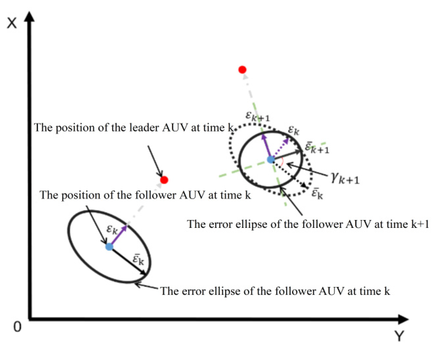
For the single master–slave AUV cooperative navigation system, after one acoustic measurement from the slave AUV, let the positioning error in the direction of the acoustic measurement from the slave AUV be $\epsilon$ and the positioning error in the longitudinal axis of the acoustic measurement direction be $\overline{\epsilon }$. Then, the positioning error from the slave AUV can be expressed by the ellipse error, where $\epsilon =\sigma$. Let the errors from the slave AUV at time k be ${\epsilon }_k$ and ${\overline{\epsilon }}_k$. Taking the position from the slave AUV as the origin and establishing the polar coordinates of the error ellipse equation, we have

$$r^2=\frac{{\overline{\epsilon }}_k^2{\epsilon }_k^2}{{\overline{\epsilon }}_k^2{\sin }^2\beta +{\epsilon }_k^2{\cos }^2\beta }$$

(14)

where r is the modal length of the error vector from the origin to any point on the error ellipse and $\beta$ is the angle between this error vector and the horizontal axis of the error ellipse.

At time k + 1, as shown in Figure 4, the error propagation equation for multi-AUV cooperative navigation is obtained by combining the polar equation of the error ellipse Equation (14) as

$$\{\begin{array}{l}{\overline{\epsilon }}_{k+1}^2=\frac{{\overline{\epsilon }}_k^2{\epsilon }_k^2}{{\overline{\epsilon }}_k^2{\sin }^2{\gamma }_{k+1}+{\epsilon }_k^2{\cos }^2{\gamma }_{k+1}}+\xi \cdot \Delta t\hfill \\ {\epsilon }_{k+1}^2={\epsilon }_0^2\hfill \end{array}$$

(15)

where $\xi$ is the error propagation growth factor related to the velocimetric accuracy of the DVL that is carried from the slave AUV. The absolute value ${\gamma }_{k+1}=|{\theta }_k-{\theta }_{k+1}|$ is the directional angle difference between two adjacent acoustic measurements; ${\epsilon }_0^{}$ depends on the measurement accuracy of the acoustic equipment.

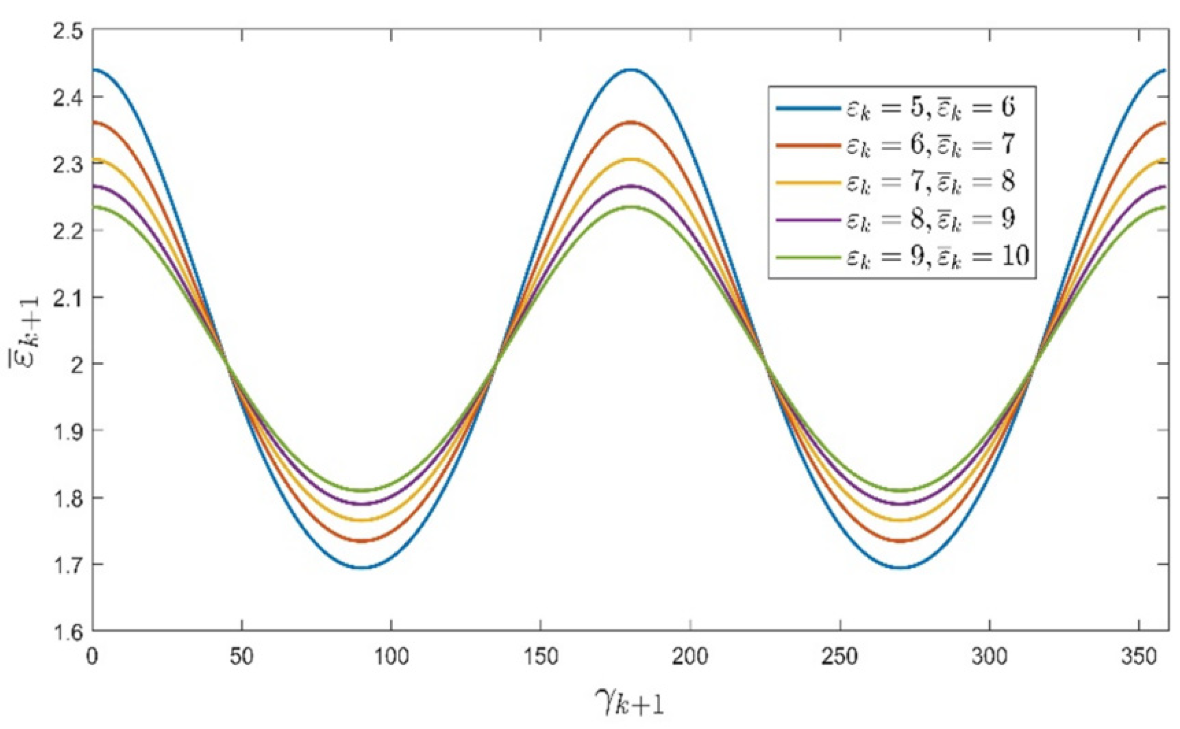
From Equation (15), it can be seen that the errors are accumulating due to the acoustics in the longitudinal direction of the measured values, i.e., ${\overline{\epsilon }}_k>{\epsilon }_k$. To analyze the multiple error propagation characteristics, the relationship between ${\overline{\epsilon }}_{k+1}$ and ${\gamma }_{k+1}$ was analyzed, as shown in Figure 5.

As depicted in Figure 5, the positioning error is minimal when ${\gamma }_{k+1}={90}^{\circ }$ or ${\gamma }_{k+1}={270}^{\circ }$. The results of the error analysis are consistent with the results of the analysis of the observable measures in this paper [15].

3. Cooperative Navigation Algorithm Based on a Single Master-Slave AUV

For a single master–slave AUV cooperative navigation system, we propose a Markov decision process (MDP)-based cooperative navigation method, and a co-navigation algorithm based on the temporal difference (TD) method was designed. Finally, the effectiveness of the designed master AUV path planning method was verified by simulation.

3.1. Markov Decision Process

The Markov decision process (MDP) means that the decision-maker periodically or continuously observes a stochastic dynamic system with Markovian characteristics and makes decisions in a sequential manner [30,31]. The MDP contains a set $S$ of environmental states, a set $A$ of agents’ actions, a state transfer probability matrix $P_{sa}$, and a reward function $R$. The agent chooses the next moment of the action by interacting with the environment, which is based on the state of the environment, and the states change and generate reward values. The core idea of reinforcement learning is to find a policy $\pi$ for the agent, i.e., a sequence of actions that maximize the cumulative value of the designed reward function, in order to obtain the optimal policy, the process of which is shown in Figure 6.

The MDP consists of the following 4 components:

$$M=(S,A,P_{sa},R)$$

(16)

where state-space $S=\{s_1,s_2,s_3,\dots ,s_n\}$ is the set of actions $A=\{a_1,a_2,a_3,\dots ,a_m\}$. The state transfer matrix P_sa is given by the following conditions:

$$p(s^{\prime },r|s,a)=\mathrm{Pr}\{S_t=s^{\prime },R_t=r|S_{t-1}=s,A_{t-1}=a\}$$

(17)

Similarly, the optimal action-value function for the optimal strategy is

$$q_{*}(s,a)=\underset{\pi }{\max }{q}_{\pi }(s,a),s\in S,a\in A(s)$$

(18)

3.2. Master AUV Path Planning Method for a Single Master-Slave AUV Based on the TD Method

The temporal difference (TD) method is a model-free reinforcement learning method that was proposed by Sutton in 1988. The TD method is necessarily convergent under the condition of a decreasing learning rate [32,33,34,35]. The multi-AUV cooperative navigation system needs to break through the underwater communication limitations, load restrictions, and interference in the complex ocean environment to propose a navigation method that meets the formation and mission requirements within the constraints [36]. The reinforcement learning method does not require a complete mathematical model but can solve the communication limitation problem, which can lay the foundation for AUV cooperative formation and clustering research.

The iterative sub-equation of the value function for the TD method is as follows:

$$V(S_t)\leftarrow V(S_t)+\alpha [R_{t+1}+\gamma V(S_{t+1})-V(S_t)]$$

(19)

$$Q(S_t,A_t)\leftarrow Q(S_t,A_t)+\alpha [R_{t+1}+\gamma Q(S_{t+1},A_{t+1})-Q(S_t,A_t)]$$

(20)

where $0\le \alpha \le 1$ is the coefficient of the iteration step and $V(S_t)$ and $Q(S_t,A_t)$ are the state value and action-value function, respectively.

According to the current state s, the corresponding optimal decision ${\pi }_{*}$ is selected to be executed

$$a^{*}=\underset{a^{\prime }\in A(s)}{\arg \max }{Q}^{*}(s,a^{\prime }),s\in S$$

(21)

The TD method chooses the action $S^{\prime }$ that maximizes $Q(S^{\prime },a)$ based on the state $A^{\prime }$ to update the following value function:

$$Q(S,A)\leftarrow Q(S,A)+\alpha [R+\gamma \underset{a}{\max }Q(S^{\prime },a)-Q(S,A)]$$

(22)

The flow of the TD method is as follows.

The flow of the TD method:

Inputs: number of iteration rounds T, set of states S, set of actions A, step size $\alpha$, decay factor $\gamma$, exploration rate $ϵ$ Output: Values corresponding to all states and actions Q Initialize the value Q corresponding to all states and actions to a random value Repeated execution

Selecting actions A according to $ϵ$ greedy method   Execute action A at the current state S, and get reward R and new state S′   $Q(S,A)\leftarrow Q(S,A)+\alpha [R+\gamma {\max }_{a}Q(S^{\prime },a)-Q(S,A)]$

$S\leftarrow S^{\prime }$; Until the end state is reached.

The method solves the multi-AUV cooperative navigation problem without the determination of P_sa. The reasonableness of the modeling directly determines whether the learning training process converges and the learning results.

(1)

State set S

State set S includes the following: at time k, the heading angle ${\psi }_k^m$, navigation speed $v_k^m$, and position coordinates $(x_k^m,y_k^m)$ of the master AUV; the heading angle ${\psi }_k^s$, navigation speed $v_k^s$, and position coordinates $(x_k^s,y_k^s)$ of the slave AUV; the relative distance measurement ${\widehat{d}}_k^s$ between the AUVs; and the relative azimuth measurement ${\widehat{\theta }}_k^s$. S can be expressed as

$$S\in \{{\psi }_k^m,v_k^m,(x_k^m,y_k^m),{\psi }_k^s,v_k^s,(x_k^s,y_k^s),{\widehat{d}}_k^s,{\widehat{\theta }}_k^s\}$$

(23)

Considering that the positioning error from the AUV is mainly affected by the angular variation of the relative distance measurement, the selected state set S is

$$S=\{{\widehat{\theta }}_k^s,{\widehat{d}}_k^s\}$$

(24)

To solve the problem in a limited dimension, the state quantities are discretized in the state set A.

(2)

Action set A

The action set A can be taken as a subset of the set that is obtained by discretizing the heading angular velocity ${\omega }_k^m$ of the master AUV:

$$A\in \{{\omega }_{min}^m,\dots ,{\omega }_{max}^m\}$$

(25)

(3)

Reward set R

The theoretical localization error of the slave AUV is taken as the cost $C_k^s$ generated by the master AUV performing each action, i.e.,

$$C_k^s={({\overline{\epsilon }}_k^s)}^2+{({\epsilon }_k^s)}^2$$

(26)

In addition, a suitable distance must be maintained. Define the minimum and maximum safe working distances $D_{\min }$ and $D_{\max }$ DVL, respectively. Define the master AUV penalty function $P_k^s$ as

$$P_k^s=\{\begin{array}{ll}{e}^{\left(c(D_{\min }-D_k^s)-1\right)},\hfill & D_k^s\le D_{\min }\hfill \\ 0,\hfill & D_{\min }\le D_k^s\le D_{\max }\hfill \\ e^{\left(c(D_k^s-D_{\max })-1\right)},\hfill & D_k^s\ge D_{max}\hfill \end{array}$$

(27)

where c is the penalty coefficient.

According to Equations (26) and (27), the reward resulting from the action that is performed by the master AUV at time k is

$$R_k=-{\displaystyle \sum _i(C_k^i+P_k^i)},\hspace{0.17em}\hspace{0.17em}\hspace{0.17em}i=1,2,\dots$$

(28)

In summary, the master AUV path planning method based on the TD algorithm for a single master–slave AUV is as follows:

(1)

Input the route and parameters of the slave AUV;

(2)

Obtain the discrete set of system states by Equation (24) and the discrete set of actions by Equation (25);

(3)

Train the master AUV using the TD method. The instantaneous reward for the master AUV to act is calculated by Equation (28), and the optimal action-value function is obtained after completing the training;

(4)

Initialize the master AUV state. Make the optimal decision using Equation (21) and obtain the planned optimal path.

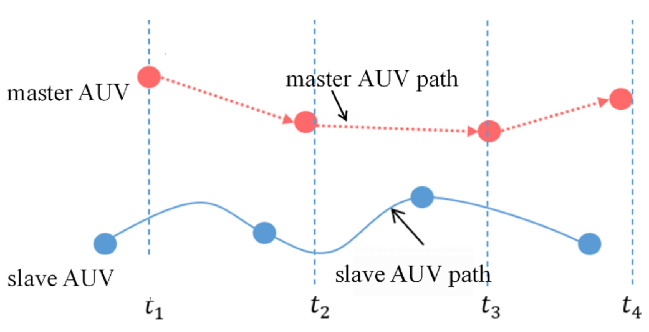
A schematic of multi-AUV cooperative navigation is shown in Figure 7. The continuous motion path is divided into points with a fixed period after time discretization. These points are also the communication nodes. At time t, the master AUV and the two slave AUVs communicate with each other acoustically to obtain the relative distance value and the relative bearing value, which is the current system state S. Next, the master AUV selects the best action of a* to execute from the best action-value function that is obtained through learning, and the system state changes to S’. The above process is repeated at each subsequent acoustic communication node to obtain the optimal path of the master AUV.

3.3. Simulation of Master AUV Path Planning Based on the TD Method for a Single Master–Slave AUV System

(1)

Simulation parameters

The parameters of the relevant navigation equipment carried by the master and slave AUVs are set as in

Table 1. Master and slave AUV-related parameters.

Parameter	Master AUV	Slave AUV
Speed measurement noise	0.5	1.5
Navigational angular velocity measurement noise (rad/s)	0.1	0.5
Acoustical measurement noise (m)	8	8
Acoustical measurement period (s)	10	10

.

Before using the TD method for path planning, the relevant state quantities also need to be discretized. The relative distance measurement azimuth between AUVs is discretized into 36 intervals at an interval of 10°. The communication range between AUVs is [0, 900] m, according to the effective range of the acoustic measurement equipment, and every 300 m is an interval of 100 to 900 m for a total of five states.

The A of the master AUV is the heading angular velocity, and the actual AUV can be 0.08 rad/s, so the action set is selected as follows:

$$\mathrm{A}=[-0.08,-0.05,-0.03,0.00,-0.03,-0.05,0.08]$$

(29)

According to several tests to obtain the best results of the parameters, define the parameters that are associated with the R function for the TD method in

Table 2. The R function for the TD method.

Parameter	Symbol	Value
Error propagation factor	$\xi$	0.1
Acoustical ranging accuracy	${\epsilon }_0^{}$	1
Penalty factor	$c$	0.06

.

Given the above parameters, it is also necessary to determine the parameters that are related to the TD method, mainly the learning step $\alpha$, the decay factor $\gamma$, and the exploration rate $ϵ$, according to several experiments to obtain the best results of the parameters are shown in

Table 3. Parameters related to the TD method.

Parameter	Symbol	Value
Learning step	$\alpha$	0.015
Decay factor	$\gamma$	0.9
Exploration rate	$ϵ$	0.1

.

(2)

Simulation analysis

Simulation tests were designed for three sets of a single master–slave cooperative navigation scenario as an example, in order to compare and analyze the effectiveness of the master AUV path plan based on the TD method with the relative distance variation and the theoretical error that were calculated by Equation (15) as indicators, which specify that the paths of the slave AUVs and master AUVs are straight and curved paths, respectively.

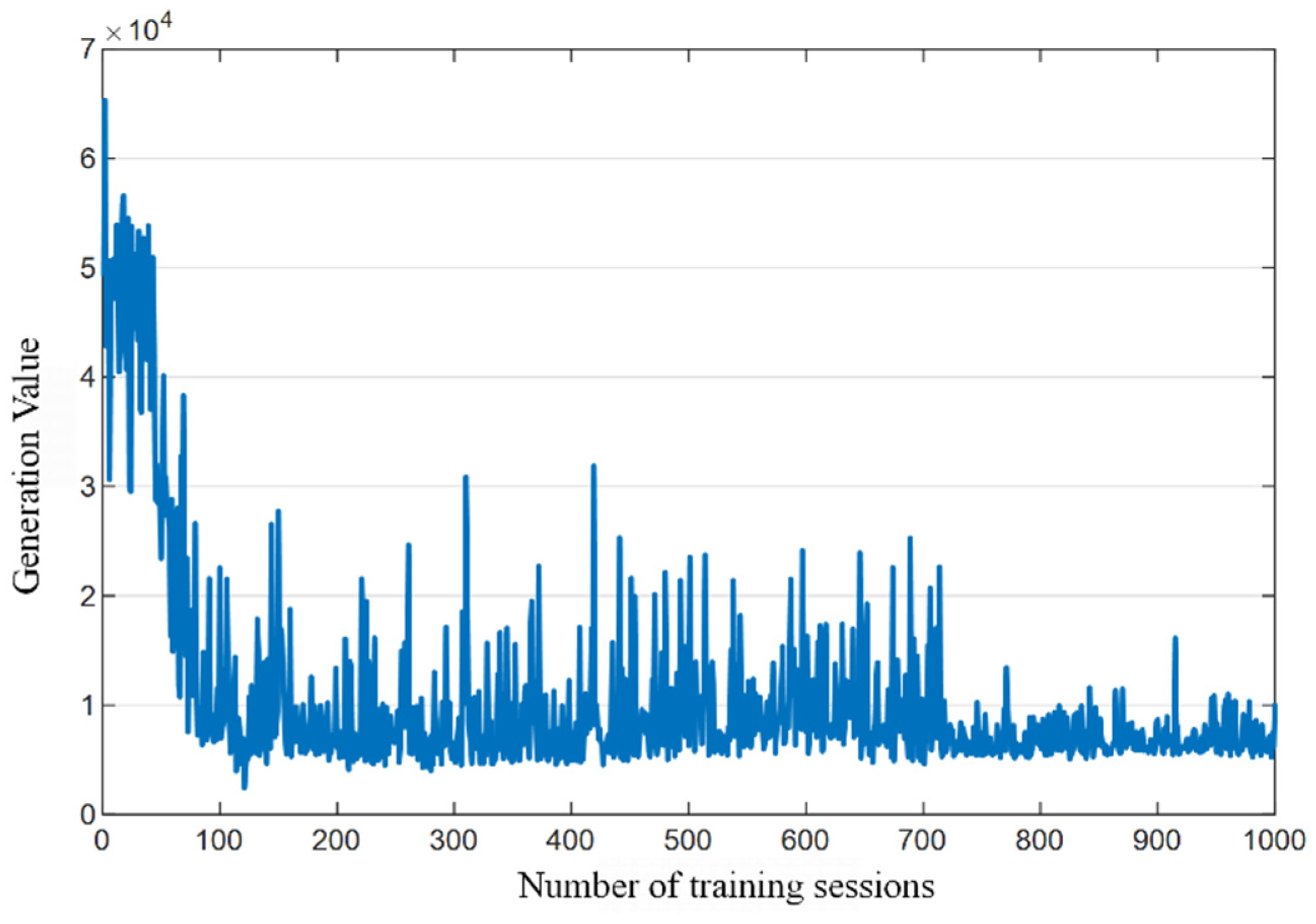
First, the slave AUV path was set as a uniform linear motion, and the slave AUV moved northward from (0, 0) with a velocity of 1.5 m/s. Three master AUVs were designed as a control group. Master AUV₁ based on the TD method started from (50, 50) with a speed of 2 m/s; master AUV₂ moving along a straight-line path started from (100, 0) with a speed of 1.5 m/s; master AUV₃ moving along a sinusoidal curve path started from (0, 100) with a speed of 1.5 m/s. The simulation time was 4000 s, and acoustic measurements were made every 10 s between the master and slave AUVs, with a maximum number of training sessions of 1000.

After 1000 training sessions, the change in the observed angle generation value is shown in Figure 8.

As shown in Figure 8, the generation values begin to converge, starting from the 100th iteration of training; they then stabilize in the subsequent training process. Although fluctuations occur, the master AUV continues to explore the environment while learning the optimal strategy, which is within the acceptable range. The action-value function is obtained after training, and then the final action is selected according to Equation (21) to obtain the planned path, as shown in Figure 9.

In Figure 9, the path of the blue master AUV₁ was obtained by the TD method, and the paths of AUV₂ and AUV₃ were obtained by manual planning as the comparison group. It can be seen from Figure 9 that both AUV₁ and AUV₂ ensure a large relative observation angle change as much as possible by constantly maneuvering to reduce the colocation error from the AUV. The straight path of AUV₃ always keeps a fixed observation angle and makes it unobservable, and the path cannot reduce the positioning error from the AUV.

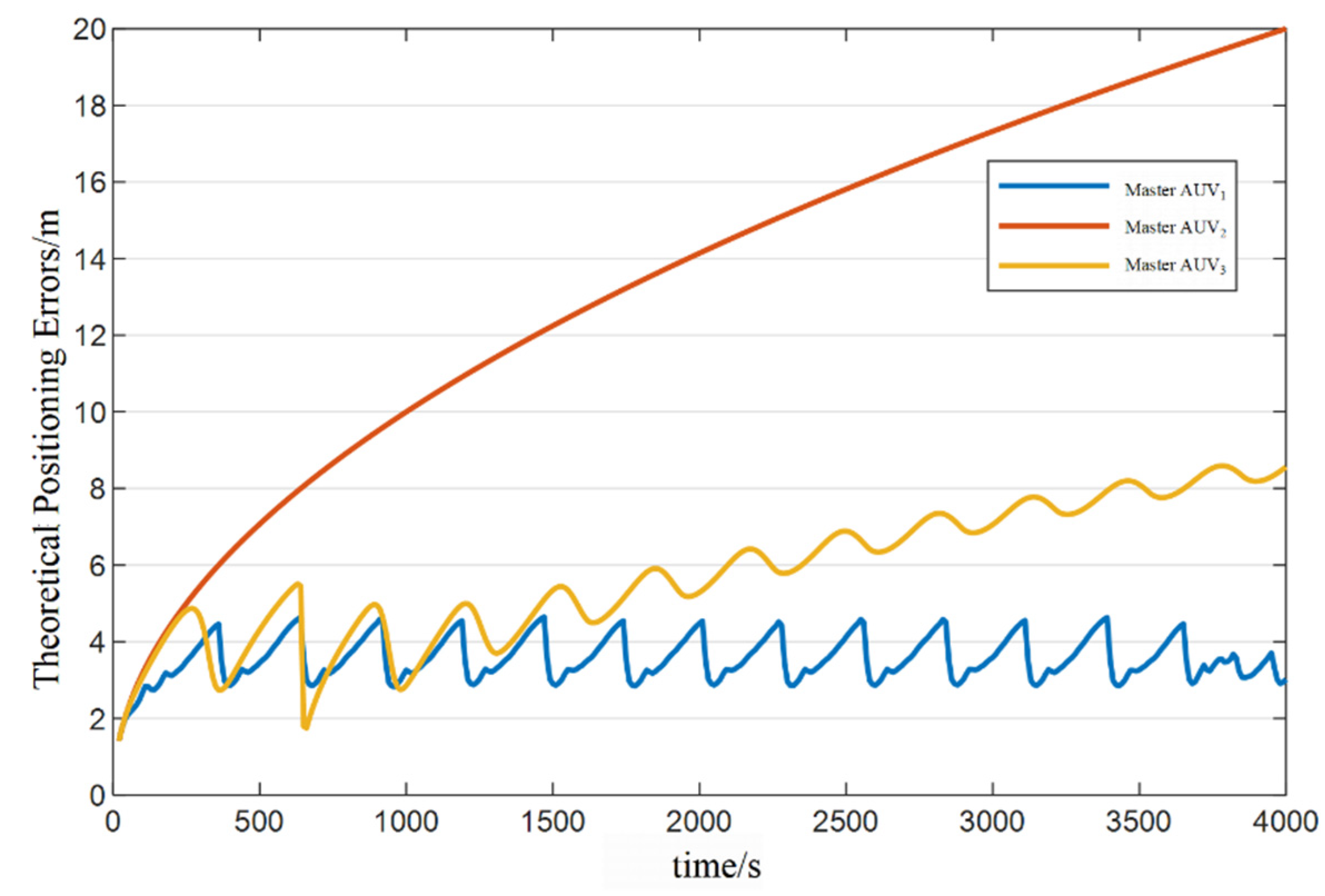
Next, the theoretical positioning errors of the three master AUVs that are calculated by the error propagation Equation (15) are compared and analyzed. The change in theoretical positioning errors between the master and slave AUVs is shown in Figure 10.

To more clearly describe the theoretical positioning errors between the master and slave AUVs in Figure 10, the information is shown in statistical form in

Table 4. Theoretical positioning errors of the AUVs.

Master AUV	Max/m	Min/m	Average/m
AUV1	4.649	1.414	3.543
AUV2	20	1.414	13.389
AUV3	11.214	1.414	8.042

.

Comparing the results in Figure 10 and Table 4, it can be seen that the theoretical positioning error of master AUV₁ that is obtained by the TD method is the smallest and is convergent during the whole navigation period. AUV₃, which travels according to the sinusoidal curve path, has an increasing positioning error after the start of navigation for 1000 s. This is because, as the distance between AUVs increases, the amount of change in the relative observation angle decreases, and the error accumulates and increases. AUV₂ has the weakest observability because it adopts a straight-line path that is parallel to the AUVs, so the positioning error continues to increase and diverge. It can be seen that the path that is planned by the TD method can reduce the slave AUV positioning error and always maintains the appropriate distance.

4. Cooperative Navigation Simulation Test

In a cooperative navigation system, after the paths of the master and slave AUVs are determined, the slave AUVs also need to correct their positions by using relevant filtering algorithms. In this paper, based on the master AUV path planning method, the EKF nonlinear filtering algorithm was employed to design a multi-AUV cooperative navigation method and simulation tests, and the results and data were analyzed.

4.1. A Harvester Route-Based a Single Master–Slave AUV Cooperative Navigation System

This section describes simulation tests that were designed based on cooperative navigation of a single master–slave AUV system. The navigation simulation test is divided into two processes: the path planning process and the navigation calculation process, as shown in Figure 11. First, the nonlinear filtering algorithm is added to the previous master AUV path planning method, and the path of the slave AUV is planned as a harvester path that is similar to the harvester route. Then, simulation tests were designed based on the slave AUV path, and two typical nonlinear filtering algorithms, EKF and UKF, which were used to verify the performance in a single master–slave AUV cooperative navigation system based on curved routes. Finally, the experimental results and data were analyzed and discussed.

Table 5. Parameters related to the navigation simulation tests.

	Velocity Measurement Noise (m/s)	Navigation Angular Velocity Measurement Noise (Rad/s)	Water Sound Measurement Noise (m)
Master AUV	$N(0,{0.5}^2)$	$N(0,{0.1}^2)$	$N(0,8^2)$
Slave AUV	$N(0,{1.5}^2)$	$N(0,{0.5}^2)$

shows the relevant parameters that were selected in the EKF and UKF navigation simulation tests.

In Table 5, according to the actual situation of the cooperative navigation system, the measurement noise that is associated with the high-precision and high-cost navigation equipment carried by the master AUV is smaller, and the measurement noise of the slave AUV is larger. Finally, the AUVs use the same acoustic measurement equipment, so the acoustic measurement noise is the same, and all the above noises are zero-mean Gaussian white noise.

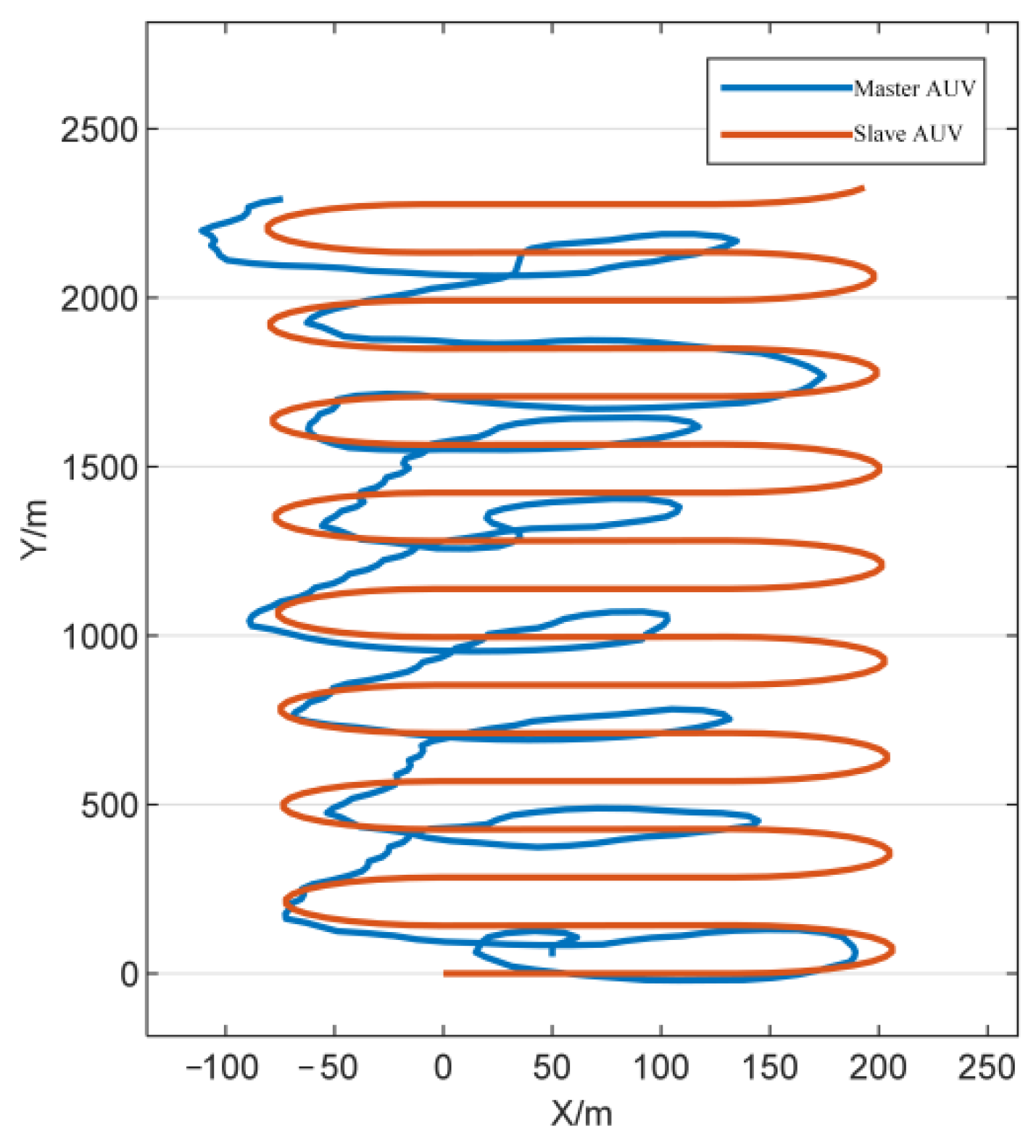
4.2. Path Planning Analysis

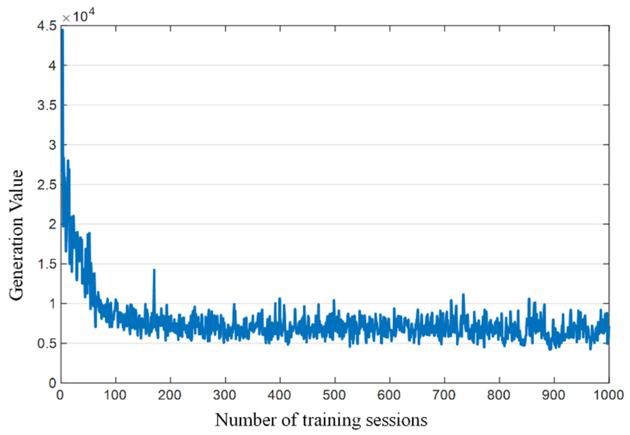
The first is the path planning process. The designed slave AUV path is from the point (0, 0), with a uniform curve motion along the harvester route to the north with a navigation speed of 1.5 m/s. The master AUV starts from point (50, 50) with an initial heading angle of $\pi /2$ and a navigation speed of 1.5 m/s. The simulation time was 4000 s, and the master AUV adopted the uniform path planning method that was designed in this paper.

The number of training iterations was 1000, and the value of generation from the change in observation angle is shown in Figure 12.

In Figure 12, the cost from the change in observation angle gradually converges to the minimum value after the 100th training session, which is within the acceptable range. During the training process, there are fluctuations in the generation value due to the master AUV constantly exploring new decisions. The table of action-value functions is obtained after the training is completed, and the planned path of the master AUV can be obtained by continuously selecting the optimal action to execute, according to Equation (21), as shown in Figure 13.

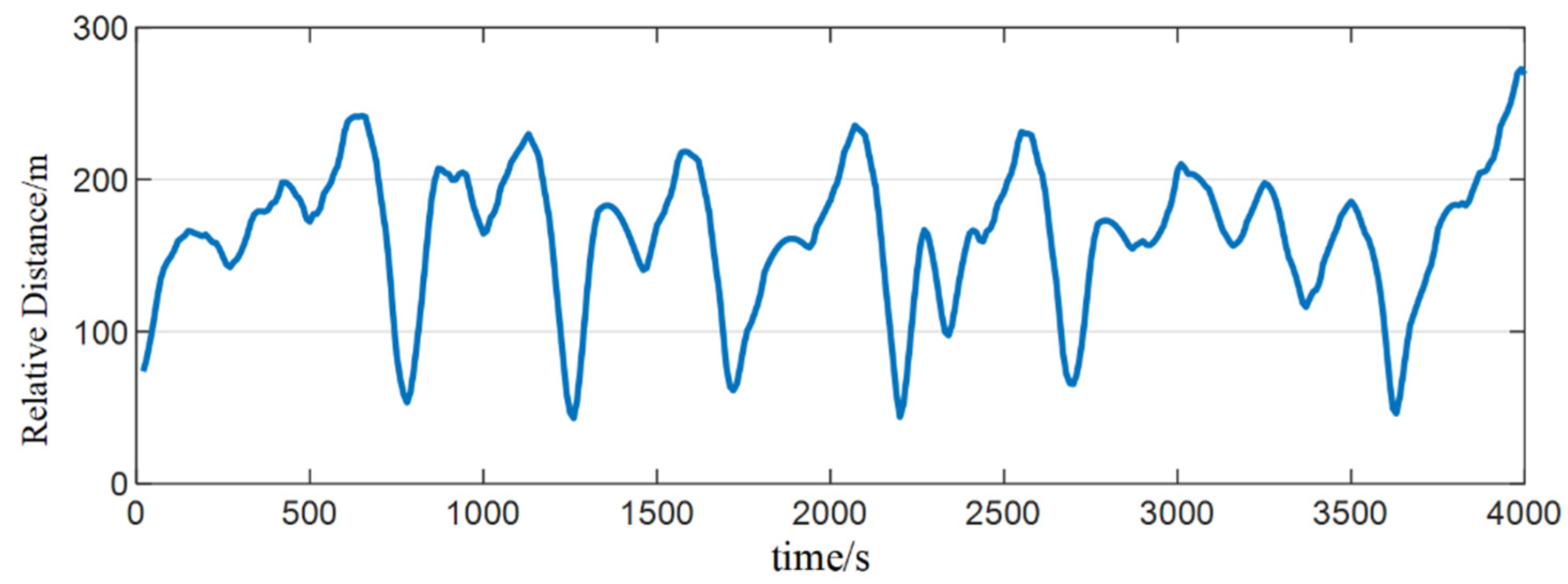
From Figure 13, it can be seen that the paths of the slave AUV follow a certain period law of harvester routes that are constantly changing, and the master AUV path that is obtained from training and learning also has a certain period law, which maintains the same harvester routes as the master AUV. The relative distance change between the AUVs during 4000 s is shown in Figure 14.

As shown in Figure 14, the maximum distance between the AUVs was 272.7 m, the minimum distance was 43.1 m, and the average distance was 164.1 m. When sailing at the same speed, a closer distance can result in a greater angular velocity change, so the master AUV tends to keep a closer distance than the slave AUV. Considering safety during navigation, a safe distance needs to be maintained between the AUVs. Therefore, the master AUV moves away from the slave AUV when the distance is too close, but it never exceeds the maximum working range of the acoustic measurement equipment, so the master and slave AUVs can always maintain a suitable distance overall.

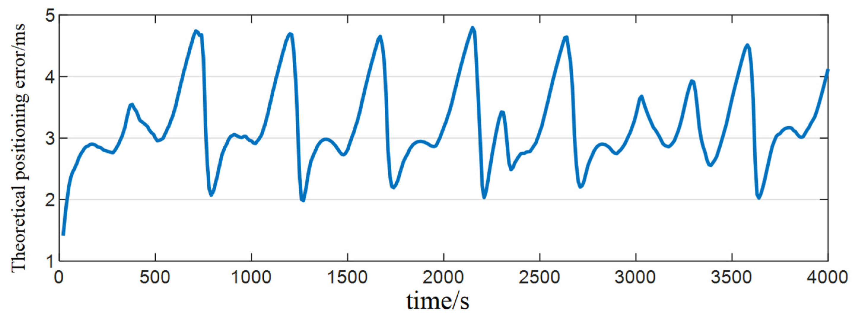
The theoretical relative distance between the master and slave AUVs is shown in Figure 15.

As shown in Figure 15, the theoretical error from the slave AUV was the smallest at the beginning of navigation, at 1.414 m. As the navigation continued, the error gradually increased, and the maximum error was 4.7966 m, which was not divergent. The average value of the error during the whole navigation period was 3.1916 m. The planned master AUV path can achieve the purpose of reducing the slave AUV positioning error.

4.3. EKF Verification

After completing the path planning process, the next step is the navigation calculation process. Two typical nonlinear filtering algorithms, EKF and UKF, were used for verification. First, the EKF algorithm was chosen to simulate the navigation calculation process, and then the simulation results were used to analyze whether the master AUV path that was planned by the algorithm in this section could achieve good results in the actual navigation process.

The path that was directly obtained from the slave AUV for DR is shown in Figure 16.

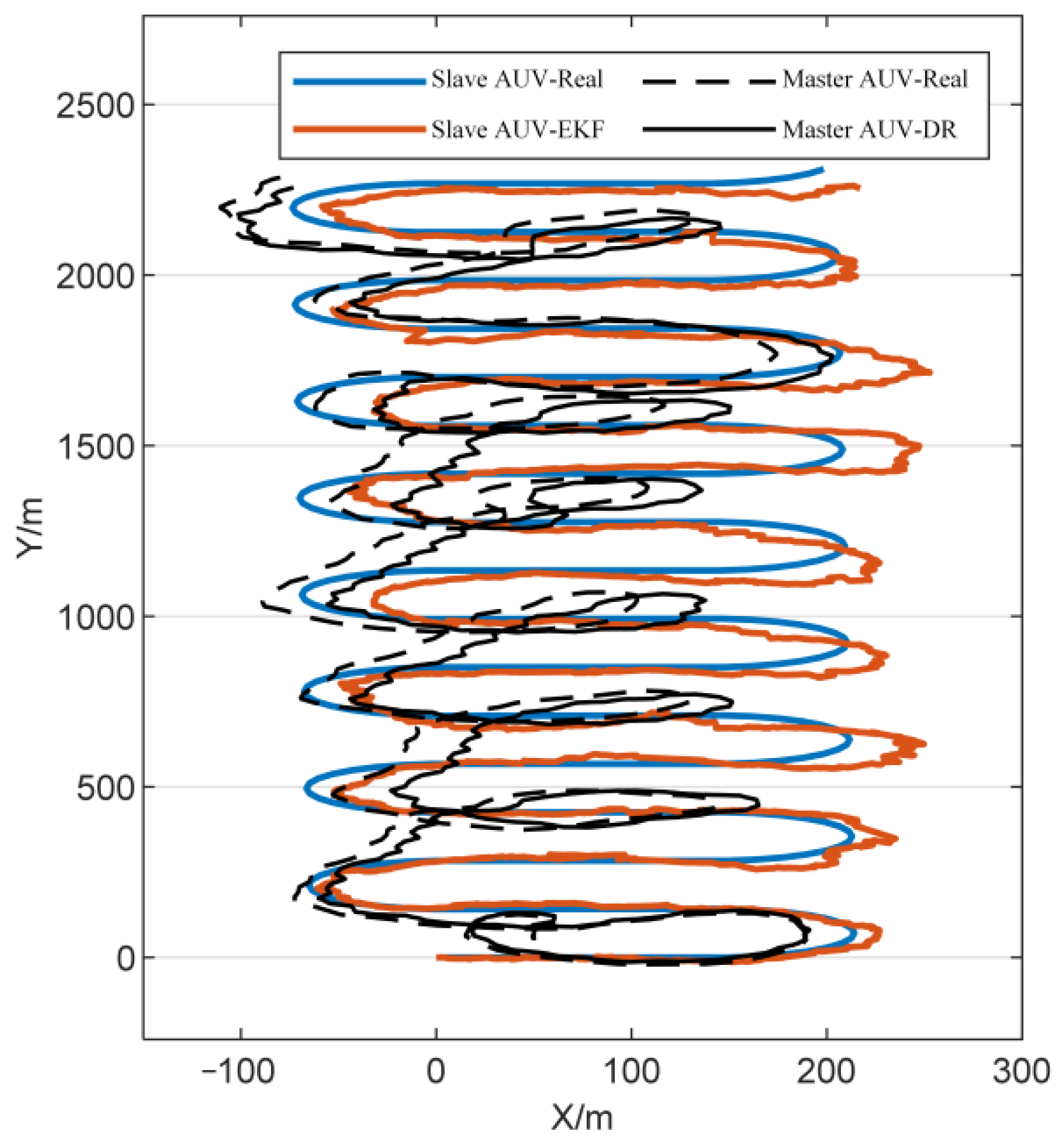
From Figure 16, we can see that the AUVs move eastward in a straight line at the beginning of the voyage, and the heading projection path is close to the true path. However, after the first turn, the heading projection path starts to lag and deviates from the true path, producing large deviations in both the X and Y axes. Then, the master AUV continues to sail according to the planned path, and the path that is obtained after the navigation calculation by the EKF algorithm is shown in Figure 17.

In Figure 17, the black dashed curve is the real path of the master AUV. To make the simulation as close to the actual situation as possible, the master AUV mainly relied on the DR for navigation and positioning during navigation. There is a large cumulative error of the acoustic equipment of the master AUV; its heading projection path is the black solid curve. After the EKF operation, the path of the slave AUV is close to the real path, but there is still some error during the turn. The positioning errors of the slave AUV during the whole navigation period are shown in Figure 17.

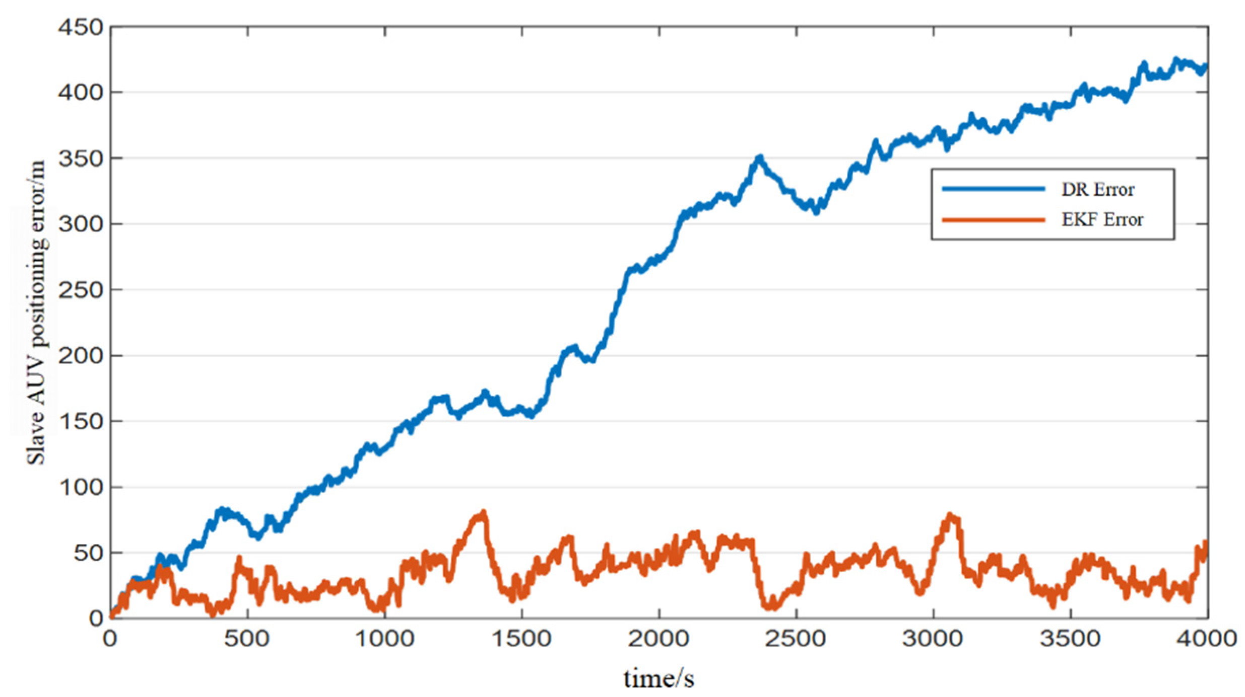
In Figure 18, the blue and red curves are the positioning errors of the slave AUV based on the DR and EKF algorithms, respectively. It can be seen that the error of the DR algorithm grows from the beginning of navigation because the error accumulates with time. During the whole navigation period, the maximum value of the error that is generated by the slave AUV through the DR algorithm is 426.04 m, and the average error is 172.81 m. After the EKF, the maximum positioning error of the slave AUV is 82.15 m, and the average error is 26.33 m. From the above analysis, it can be seen that the positioning error of the slave AUV is greatly reduced after the EKF.

4.4. UKF Verification

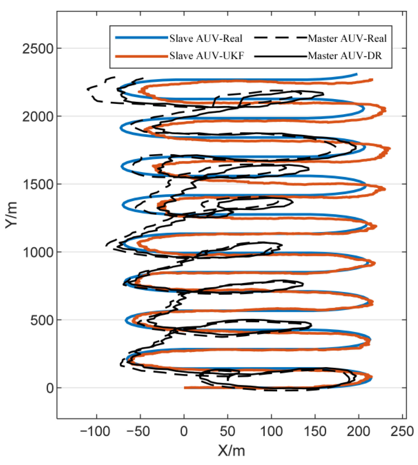
In this section, the UKF algorithm was used for a cooperative navigation analysis. The master and slave AUV paths that were obtained from the navigation calculations using the UKF are shown in Figure 19.

In Figure 19, the black dashed curve and the solid curves are the real path of the master AUV and the path of the DR, respectively. After UKF calculation, the path of the slave AUV is roughly close to the real path. In the early stage of navigation, the slave AUV path is close to its real path, but there is still some error during the turn, and the error increases with time. The positioning errors of the slave AUV during the whole navigation period are shown in Figure 20.

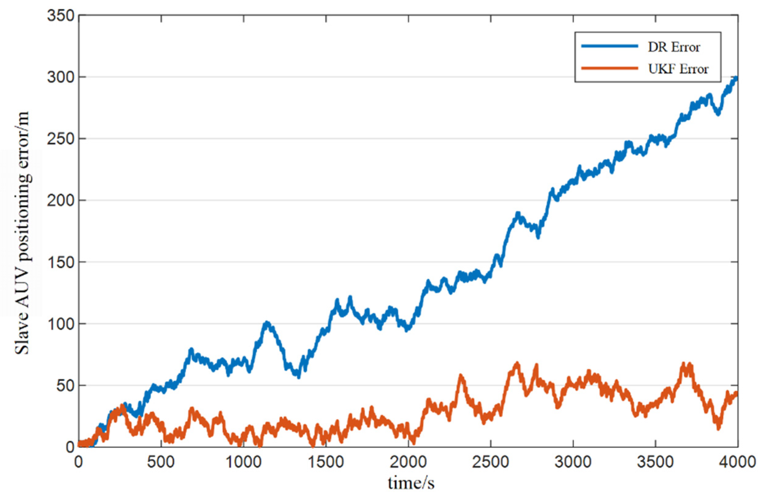
In Figure 20, the blue and red curves are the DR error and positioning error of the slave AUV, respectively. It can be seen that the DR error starts to grow with time navigation. During the whole navigation period, the maximum value of the slave AUV DR error is 300.73 m, and the average error is 97.18 m. After the UKF, the maximum position error of the slave AUV is 68.44 m, and the average error is 21.82 m.

For further analysis, 100 navigation experiments were performed using the EKF and the UKF. The statistics related to the positioning errors that were obtained are shown in

Table 6. Co-navigation test error (m).

	Average Error		Average Relative Error/m
	x-axis/m	y-axis/m
DR	26.35	85.49	155.22
EKF	16.27	29.02	51.56
UKF	16.19	28.81	51.18

below.

Table 6 shows that the error of the DR is mainly on the y-axis, regardless of the average error or the relative average error. The average error of 100 navigation tests was 85.49 m, which is much larger than the 26.35 m on the x-axis. It can also be seen that the EKF and the UKF have broadly the same effect. The simulation experiments illustrate that both filtering algorithms can effectively reduce the positioning error of the slave AUV and thus improve the positioning performance of the AUV system.

5. Conclusions

To reduce the cooperative positioning error and improve the navigation accuracy, a single master–slave multi-AUV cooperative navigation method is proposed in this paper. The path of the slave AUV is planned according to the navigation task, and the algorithm is used to plan the path for the master AUV to minimize the observation error and positioning error of the slave AUV. This method divides the whole cooperative navigation process into the path planning process and the navigation calculation process. In the path planning process, the MDP model of the cooperative navigation problem is first established for the single master–slave AUV system. Then, the master AUV path planning method is designed based on the TD method, and the effectiveness of the method is analyzed by simulation tests. The results show that the theoretical positioning error of the slave AUV can be controlled to about 3.2m by planning the path of the master AUV using the TD method. In the navigation calculation process, the path planning method is combined with two nonlinear filtering methods, the EKF and UKF. The simulation test of the single master–slave AUV cooperative navigation system based on the harvester route was designed to further verify the feasibility and effectiveness of this method. The experimental results show that the proposed method can effectively solve the problem of restricted underwater communication and lays a foundation for future formation applications, such as cluster-oriented and cooperative communication.

There are still some aspects to be improved in the future; for example, appropriately increasing the number of slave AUVs—a single master–multiple slave AUV system may improve the navigation accuracy of the system. Considering the delay time of ocean currents and acoustic communication has the potential to improve the robustness of the algorithm.