Hydrodynamic and Flow Field Characteristics of Water Jet Propulsion under Mooring Conditions

Abstract

The acceleration characteristics of a water jet-propelled ship during startup are related to its performance under mooring conditions. Water jet propulsion cavitation during startup increases the vibration and noise of the whole ship. Therefore, accurately predicting and analyzing the performance, hydrodynamics and flow field characteristics of water jet-propelled ships under mooring conditions can help elucidate the startup characteristics of the ships and optimize their acceleration strategies. In this study, the hydrodynamic and flow field characteristics of water jet propulsion and water jet propulsion ships under mooring conditions were studied using three-dimensional numerical modeling. First, the hydrodynamic performance of the water jet propeller was analyzed, and the relevant flow field law was derived. Then, the hydrodynamic performance, internal and external flow field characteristics, pulsation pressure and flow rate at the nozzle, and pulsation pressure at the monitoring points around the impeller of the water jet propulsion ship model were analyzed under mooring conditions. We obtained the open-water law for the water jet propeller and the hydrodynamic force and flow field law for a two-pump water jet propulsion ship. The ship model developed in this study provides a good theoretical foundation for further research on water jet propulsion.

1. Introduction

Water jet propulsion is an advanced propulsion technology that has been rapidly developing and progressing since the 1980s. Compared with traditional propulsion, water jet propulsion is more efficient, stealthier, and exhibits a better anti-cavitation performance in high-speed conditions. The startup acceleration characteristics of water jet propulsion ships are directly related to their comprehensive performance under mooring conditions. Thus, it is meaningful to numerically predict water jet propulsion performance and analyze the changes in the flow field characteristics under mooring conditions. By developing accurate water jet propulsion models under non-design conditions, methods for predicting the performance of water jet propulsion could be enriched and designs for enhancing the performance of water jet propulsion ships could be developed.

Extensive research has been conducted on water jet propulsion and water jet-propelled ships using numerical simulations and experimental methods. Kandasamy et al. [1] performed numerical simulation studies on a water jet-propelled ship by applying the volume force method, and the numerical simulation was verified with model tests. Takai et al. [2] used the non-constant solver RANS SHIP-IOWA to simulate the performance of a water jet-propelled ship with a joint high-speed sealift design (JHSS). Duerr et al. [3] numerically predicted the inlet disk surface inhomogeneities of a real-scale water jet-propelled ship and determined the axial distribution of the incoming velocity of water jet propulsion. The upper half of the paddle disk surface axial velocity is smaller than that of the lower half of the paddle disk surface, which is similar to the phenomenon of a special point existing outside the axial velocity distribution of the flow field in the circular tube. Yang et al. [4] showed that the underwater noise of a ship driven by water jet propulsion was approximately 16 dB lower than that of a ship using a conventional propeller under the same operating conditions. Fung et al. [5] developed and evaluated a “concept ship” by implementing a conventional propeller, axial flow, and hybrid water jet propulsion pump drives. Xianlong Liu et al. [6] used the ducted propeller design method to design the impeller of the water jet propeller, used the spatial transformation method to transform the two-dimensional NACA airfoil into a three-dimensional airfoil, and established the flow field model of the water jet propeller using structured grid technology. Fan Jiang et al. [7] established a model of a trimaran driven by water jet propulsion and conducted water jet propulsion model tests in open still water.

In addition, the transient characteristics of water jet pumps significantly affect water jet propulsion characteristics under mooring conditions. Lefebvre et al. [8] concluded that quasi-steady-state assumptions could not accurately predict the transient pump hydraulic characteristics. Thanapandi et al. [9,10] showed that the transient characteristics of the water jet pump during startup under lower acceleration can be predicted to some extent using the steady-state assumption. The studies of Tsukamoto et al. [11,12] showed that both the flow and head of the pump in rapid startup fall back from the peak and below the quasi-steady-state values for some time before they start with the same pattern. This is mainly due to the hysteresis effect of the impeller speed. Moreover, the hysteresis effect of the vane winding causes the head to be much higher during rapid stopping than that of the quasi-steady-state value.

Kandasamy et al. [13] derived an integral force/moment water jet model using computational fluid dynamics (CFD). This method was applied to the DTMB 5594 ship model flow field and performance simulations. Experiments by Duplaa et al. [14,15,16] illustrated a sudden pressure drop in the late startup period; they further explored performance degradation due to system cavitation during startup. Tanaka et al. [17,18,19] carried out a visualization study of cavitation during the transient state using a high-speed camera and found a correlation between the cavitation behavior of the pump and the rapidly changing flow and pressure. Shoutian Chen et al. [20] designed a special multi-ring structure of water jet propeller nozzle based on the Coanda effect. The results show that the designed structure can effectively improve the problem of the low efficiency of water jet propellers at low speeds, which is of great significance to better the performance of water jet propellers.

Mooring conditions refer to the operation process of using mooring equipment to make the ship stop at the berth, including berthing wharf, trestle berth, pile column, mooring buoy and alongside other ships. A number of studies have been carried out on mooring conditions for marine platforms. However, studies on ships and individual propulsion are few. Zhang et al. [21] proposed a design method for the arrangement of mooring systems of ships at different water depths. Xu et al. [22] used the time-frequency domain method to calculate the motion of an offshore product tanker and its mooring position.

In summary, research on mooring conditions has mostly focused on the effects of the wind and wave currents, and the number of ships and their mooring positions. Studies on the steady-state and transient hydrodynamic characteristics and flow field characteristics during water jet propulsion pump startup focus on spiral, centrifugal, and slant flow pumps [23,24]. Moreover, they mainly involve basic theoretical studies and calculations of the steady-state and transient flow fields inside the pump and fine flow field tests particle image velocimetry (PIV) while the ship is non-stationary. There are a lack of theoretical analyses and numerical predictions of the hydrodynamic and flow field characteristics of water jet propulsion and their mooring conditions. It is necessary to conduct a three-dimensional (3D) study of water jet propulsion under mooring conditions to have a more comprehensive understanding of the hydrodynamic and flow field characteristics at different rotational speeds and to be able to develop a practical and accurate numerical prediction method for water jet propulsion.

2. Numerical Simulation Method and Calculation Formula of Water Jet Propulsion

Natural flow is under the control of conservation laws and is determined by continuity, momentum, and energy equations [25]. As the water jet propeller performance calculation does not consider heat exchange, we neglected the energy equation and carried out the flow simulation based on the Navier–Stokes equations as follows:

The continuity equation:

$$\frac{\partial \rho u_i}{\partial x_i}=0$$

(1)

The momentum equations:

$$\frac{\partial (\rho u_i)}{\partial t}+\frac{\partial (\rho u_i{u}_j)}{\partial x_j}=-\frac{\partial p}{\partial x_j}+\frac{\partial }{\partial x_j}u(\frac{\partial u_i}{\partial x_j}-\rho \overline{u_i{}^{\prime }{u}_j{}^{\prime }})-S_j$$

(2)

where $\rho$ is the density of the fluid, $u_i{u}_j$ are time average values ($i,j=1,2,3$) of the velocity component, $p$ is pressure,$u$ is the dynamic viscosity coefficient and $S_j$ is the source term [26].

The SST k-ω turbulence model was proposed by Menter [27]. This model can be used in the study of near- and far-wall problems as well as fluid–solid surface separation problems. In addition, it can accurately capture the flow phenomena at solid surfaces, suggesting that the model mesh should include the boundary layer, and has a high simulation accuracy, especially at the surface Y+ [28]. The transport equations for the turbulent kinetic energy (k) and turbulence dissipation rate (ω), respectively, are expressed as,

$$\frac{\partial k}{\partial t}+\overline{u_j}\frac{\partial k}{\partial x_j}=\frac{\partial }{\partial x_j}[(\nu +{\sigma }_k\nu )\frac{\partial k}{\partial x_j}+\widetilde{P_k}-{\beta }^{*}k\omega ],$$

(3)

$$\frac{\partial \omega }{\partial t}+\overline{u_j}\frac{\partial \omega }{\partial x_j}=\frac{\partial }{\partial x_j}[(\nu +{\sigma }_{\omega }\nu )\frac{\partial \omega }{\partial x_j}+\alpha S^2-\beta {\omega }^2+2(1-F_1){\sigma }_{\omega 2}\frac{1}{\omega }\frac{\partial k}{\partial x_j}\frac{\partial \omega }{\partial x_j}],$$

(4)

The eddy-viscosity coefficient is expressed as $v_t=\frac{a_{1}k}{\max (a_1\omega ,\Omega F_2)}$, where ${\sigma }_k=\frac{1}{F_1/{\sigma }_{k,1}+(1-F_1)/{\sigma }_{k,2}}$ and ${\sigma }_{\omega }=\frac{1}{F_1/{\sigma }_{\omega ,1}+(1-F_1)/{\sigma }_{\omega ,2}}$.

The definition of blending functions F₁ and F₂ is as follows:

$$F_1=\tanh ({\Phi }_1^4),$$

(5)

$$F_2=\tanh ({\Phi }_2^2),$$

(6)

where ${\Phi }_1=\min [\max (\frac{\sqrt{k}}{{\beta }^{*}\omega y},\frac{500\nu }{y^2\omega }),\frac{4\rho {\sigma }_{\omega 2}k}{C{D}_{k\omega }{y}^2}]$ $C{D}_{k\omega }=\max (2\rho {\sigma }_{\omega 2}\frac{1}{\omega }\frac{\partial k}{\partial x_j}\frac{\partial \omega }{\partial x_j},{10}^{-10})$, ${\Phi }_2=\max (\frac{2\sqrt{k}}{{\beta }^{*}\omega y},\frac{500\nu }{y^2\omega })$ $\widetilde{P_k}=\min ({\mu }_t\frac{\partial \overline{u_j}}{\partial x_j}(\frac{\partial \overline{u_i}}{\partial x_j}+\frac{\partial \overline{u_j}}{\partial x_i}),10\cdot {\beta }^{*}\rho k\omega )$.

The constant coefficients $\phi$ in the aforementioned equations, (k) and (ω), are calculated by

$$\phi ={\phi }_1{F}_1+{\phi }_2(1-F_2),$$

(7)

In this study, the turbulence model and control equations were discretized according to the second-order windward form finite volume strategy. The discretization form of the time term used the second-order implicit form, and the velocity–pressure utilization coupling was conducted using the SIMPLE strategy [23].

The efficiency of the propulsion pump under mooring conditions was obtained using the following equations:

Pump head:

$$H=\frac{P_2-P_1}{\rho g}+\frac{V_2^2-V_1^2}{2g},$$

(8)

where P₂ and P₁ are the surface average pressures at the outlet pressure measurement section and upstream pressure measurement section, respectively, and V₂ and V₁ are the surface average axial velocity at the inlet pressure measurement section and upstream pressure measurement section, respectively.

Power:

$$N=2\pi nM,$$

(9)

where n is the pump shaft speed and M is the impeller subjected to torque (Nm).

Efficiency:

$$\eta =\frac{\rho gQH}{N},$$

(10)

where ρ is the density, g is the acceleration of gravity, Q is the flow rate, H is the head, and N is the power.

3. Numerical Simulation Design

3.1. Water Jet Propulsion Calculation Model

Existing models in the market were selected for the water jet propeller. A water jet propeller is shown in Figure 1. The number of blades of the guide vane and impeller of the water jet propulsion system are 11 and 6, respectively. The scaling ratio λ is 16, and the impeller, guide vane, and runners are geometrically similar to each other. The specific propeller and model parameters are listed in

Table 1. Water jet propeller model parameters.

	Models	Full Scale
Impeller diameter D (m)	0.117	1.877
Diameter of nozzle (m)	0.084	1.357
Width of inlet (m)	0.134	2.149

.

As shown in Figure 2, the range of the calculation domain is 30D × 10D × 8D. Further, the calculation domain is divided into three parts: guide vane, impeller rotation, and inlet water channel domains. The nozzle and computational domain outlet were set as the pressure outlet, and the computational domain inlet is set as the velocity inlet. The other calculation domain surfaces, water jet propulsion pump wall, guide vane, and impeller surface were set to the no-slip wall surface. The Y+ value selected for the calculations in this study is 60; a non-structural grid was applied to each regional component of the water jet propeller.

3.2. Calculation Model of Water Jet Propulsion Ship

The water jet-propelled ship model used in this study is shown in Figure 3. Figure 4 shows the V-shaped semi-skid type ship, with the two water jet propellers symmetrically arranged at the stern. The layout of the pump is also shown in Figure 4. The ship model and water jet propeller scaling ratio is 16. The water jet propeller parameters are summarized in

Table 2. Parameters of the water jet propulsion model for the mooring test.

	Model	Full Scale Ship
Ship hull
Lpp (m)	6.670	106.7
Draught (m)	0.240	5.840
Drainage capacity $\nabla$ (m3)	0.549	2249
Wet surface area Sw (m2)	5.453	1396

.

To improve the computational efficiency, numerical simulations were carried out in this study for the port side of the ship model, and a water jet propeller was installed on the half of the ship model used for numerical prediction, as shown in Figure 5.

In the simulation, the calculation area was in the 3D coordinate system O-XYZ, and the XYZ directional dimensions of the overall calculation domain were set as X ∈ [−3L_pp, 3L_pp], Y ∈ [0, 2L_pp], and Z ∈ [−2L_pp, 1L_pp]. Figure 5 shows the specific boundary conditions of the computational domain of the mooring model. The inlet, lower bottom surface, upper top surface, and side of the computational domain were set as the velocity inlet and the outlet was set as the pressure outlet. In addition, the longitudinal plane (Y = 0) in the ship model was set as the symmetry plane, and all parts of the ship model and water jet propulsion system (i.e., inlet channels, rotating members, and nozzles) were set as no-slip wall surfaces.

We used a non-structural grid for the calculation, and the transition was completed using step-by-step encryption, as shown in Figure 6. The total thickness of the boundary layer δ was calculated using the flat plate theorem [29], whereas five prismatic layer grids (sum equal to δ) were set on the lower surface of the ship model to realize the boundary layer prediction of the flow field under the ship model. To achieve an accurate simulation of the internal flow of the water jet propulsion system, it is necessary to complete structural surface mesh refinement and feature line encryption for the impeller and other components of the system in turn, as shown in Figure 6c,d. In addition, the rotating domain wrapped by the flow channel needs to be encrypted locally by the body grid (Figure 6b), and a ring-shaped refinement region is set for the gap position of the flow channel and the leaf tip. Finally, the exterior Y+ of the water jet propulsion ship model was determined to be 60. The overall grid, fluid domain grid, and rotating domain grid have a total of 13.12, 11.12, and 2 million grids, respectively.

4. Verification Analysis

4.1. Water Jet Propeller Verification Results

Three different sparsity meshes (coarse, medium, and fine) of the water jet propeller were used. The detailed parameters are shown in

Table 3. Mesh parameters.

	Coarse	Medium	Fine
Number of meshes (M)	6.81	8.52	12.46
Total boundary layer thickness (mm)	2.1	2.1	2.1
Number of boundary layers	7	7	7

.

The thrust data obtained for different meshes and different time step operations at speed n = 2450 r/min are listed in

Table 4. Calculation results of three sets of meshes.

n (r/min)	Grid Name	ID	T (N)
2450	Coarse	S1	716.377
	Medium	S2	714.16
	Fine	S3	712.127

;

Table 5. Calculation results for different time steps.

	$∆\mathit{t}/2$	$∆\mathit{t}$	$2∆\mathit{t}$
T (N)	713.99	714.16	714.68

. Here, the sensitivity of the thrust to the degree of mesh sparsity is weak.

Based on the mesh convergence test results (

Table 6. Calculation results of grid-independent analysis.

n (r/min)	Parameters	RG	PG	UG	SC%
2450	T	0.162	9.991	7.399	−1.038

), we chose the medium mesh to perform the numerical prediction. From the calculation results of the time step, the time step has a small impact on the final results, and the calculation error is within 0.1%; thus, the calculation time step of 0.001 s was taken for the numerical calculation in this section.

4.2. Water Jet Propulsion Ship Verification Analysis

The convergence of the discrete water jet propulsion ship mesh was evaluated and verified using three different levels of mesh sparsity. The base size of the mesh was adjusted to change the mesh sparsity while maintaining the dimensions. The three different sparsity meshes were 8.36 M (coarse), 13.13 M (medium), and 22.39 M (fine).

The thrust data obtained for different meshes and different time step operations at speed n = 2450 r/min are listed in

Table 7. Calculation results of three sets of meshes.

n (r/min)	Grid Type	ID	T (N)
2450	Coarse	S1	441.25
	Medium	S2	433.32
	Fine	S3	430.72

and

Table 8. Calculation results for different time steps.

	$∆\mathit{t}/2$	$∆\mathit{t}$	$2∆\mathit{t}$
T (N)	433.04	433.32	434.56

, and the sensitivity of the thrust to the degree of mesh sparsity was found to be weak.

The results of the grid convergence analysis for a rotational speed of 2450 r/min are shown in

Table 9. Calculated results of mesh verifying convergence.

n (r/min)	Parameters	RG	PG	UG	SC%
2450	T	0.327	6.11	10.55	−2.44

. Based on the convergence analysis, a medium grid was chosen for the numerical prediction in this section. According to the calculation results of the time step, the time step has a small impact on the results, and the calculation error was within 0.3%. Thus, an impeller rotation time of 1° was used to carry out the numerical calculation.

5. Analysis of Numerical Calculation Results of the Water Jet Propeller and Water Jet Propulsion Ship

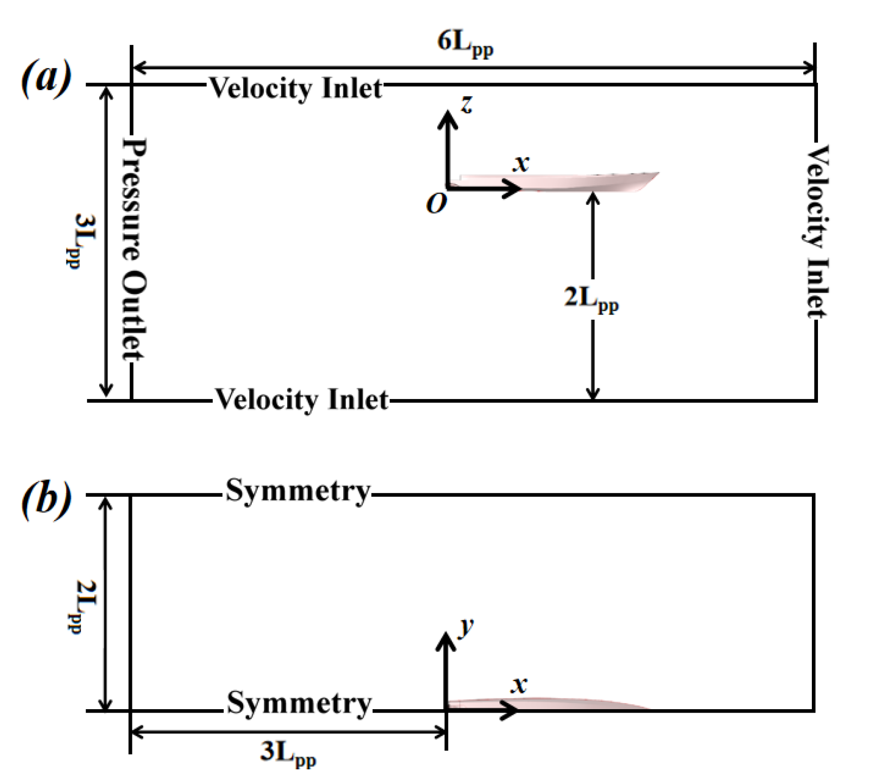
5.1. Analysis of Open-Water Performance of Water Jet Propeller under Mooring Conditions

Six speeds (i.e., 1650, 1800, 2000, 2200, 2450 and 2600 r/min) were selected for the quasi-steady-state numerical prediction conditions of the water jet propeller. Three working conditions, 1650, 2000 and 2450, were selected for the flow field analysis.

The performances of the same type of intake channel in different situations are different. The magnitude of the rotational speed under mooring conditions affects the diffusion rate of the flow and the intake channel suction capacity to some extent [25]. The inlet channel pressure distribution and outflow are not uniform due to the influence of various factors, such as inlet channel bending and propulsion pump shaft disturbance. The water jet propulsion pump inlet cross-section is the flow channel outlet cross-section, and the schematic diagram is shown in Figure 7.

Figure 8; Figure 9 show the axial velocity and total pressure distribution of the propulsion pump inlet, respectively. The high-speed distribution area and total pressure increased as the speed propulsion pump inlet cross-sectional speed increased. The velocity and total pressure around the pump shaft are symmetrically distributed. The sub-high-speed area at the top of the pump shaft corresponds to the low-pressure area shown in Figure 9. This is because of the impeding effect of the drive shaft on the water flow, making the velocity in the area around the paddle shaft lower than the area at the edge of the disk. The low-speed zone below the pump shaft corresponds to the high-pressure zone shown in Figure 9. The distribution area grows as the speed increases due to the backflow characteristics in the flow channel under mooring conditions. The larger the rotation speed, the higher the velocity gradient variation and the low-speed region range grows, which is a similar phenomenon as in the simulation of the water jet propulsion ship model. The main causes of uneven inlet and outlet flow are the effects of boundary water intake, water deceleration and return, the transition zone of the inlet channel bend, and the obstruction of the water flow by the drive shaft. The boundary water intake depends on the boundary layer intake flow, and the boundary layer intake ratio increases as the speed increases. The flow velocity gradient decreased, resulting in increased water uniformity. The drive shaft has an obstructive effect on the water flow, and there is a narrow reverse low-velocity zone around the drive shaft in the figure, affecting the uniformity of the outlet velocity distribution.

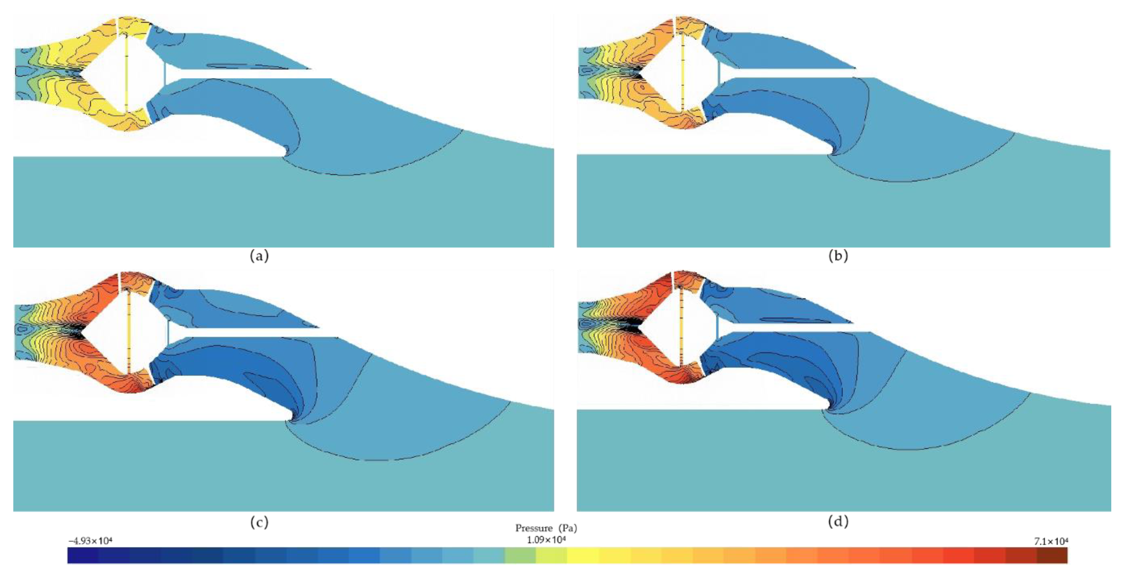
The axial velocity distribution in the middle and longitudinal sections at different rotational speeds under mooring conditions is shown in Figure 10. Some of the fluids on the lip of the flow channel experience backflow because the transition of the lip is not smooth enough and flow separation occurs. Simultaneously, the reflux phenomenon at the lower edge of the transition section of the flow channel under mooring conditions also increases the influence of flow separation. The upper side of the lip forms an apparent low-velocity zone. The axial velocity at the device flow channel inlet area is low, and the velocity increases along the pumped water flow direction. In the straight pipe area following the fluid flow into the bend, the velocity variation shows uneven velocity distributions above and below the pump shaft. Near the pump shaft, the flow velocity is low. Far from the pump shaft, the flow velocities are higher (above as well as below the pump shaft).

Figure 11 shows the pressure distribution in the middle longitudinal section along the central axis of the pump at variable rotational speeds. The pressure at the slope and lip angle changes more apparently with the rotational speed. The pressure minima in the inlet flow channel are mainly distributed at the lip angle, the bend transition, and the ramp, while cavitation may occur in combination with the flow separation condition of the return flow and the lip angle. The post-impeller region is subjected to higher pressure, which increases as the rotational speed increases. At the nozzle, the pressure distribution is not uniform because the pressure outlet is set, but all exist in the low-pressure region relative to the pump section. As the rotational speed increases, the more uniform the pressure received by the flow path.

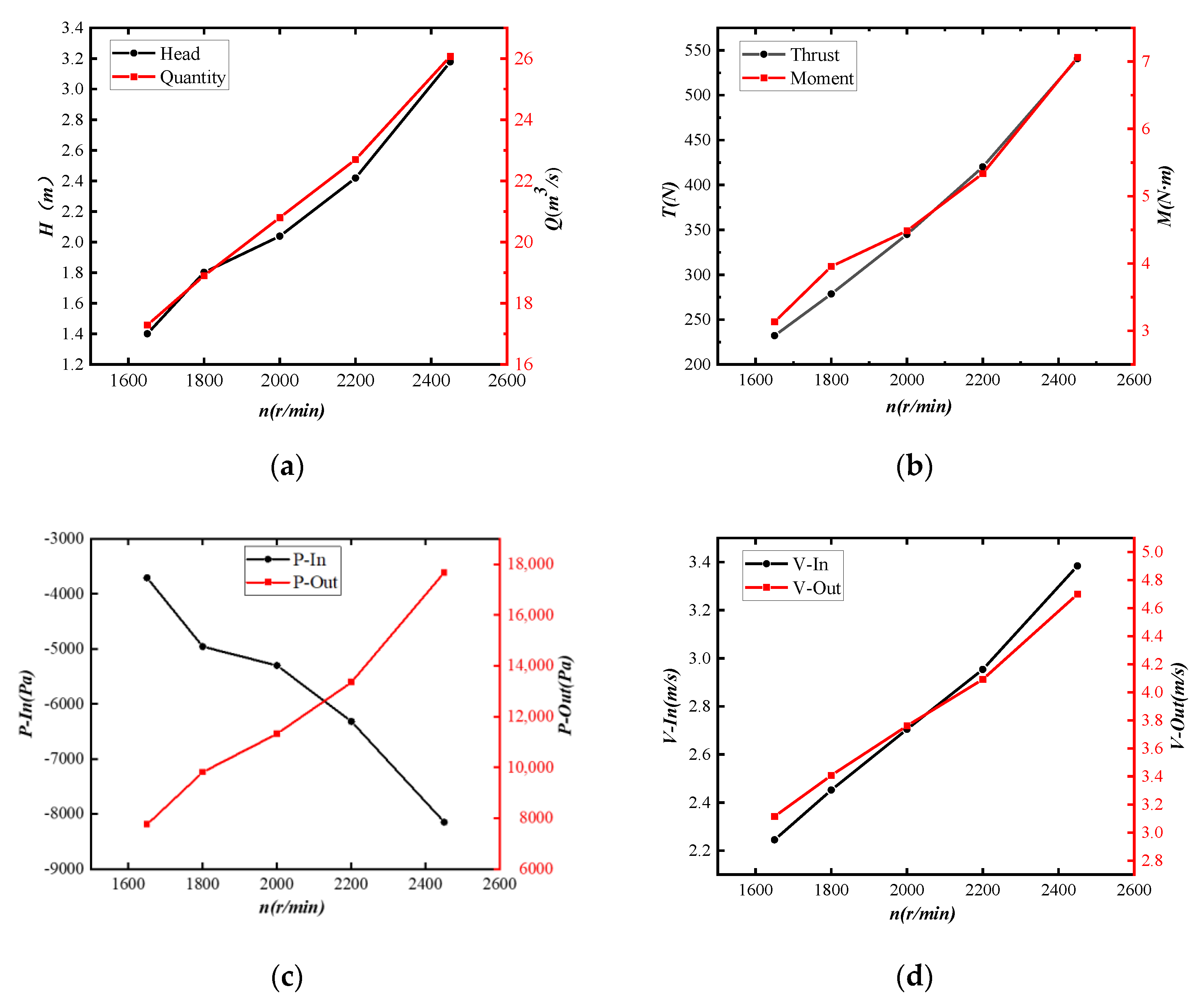
The analysis of the quasi-steady state numerical prediction of the water jet propeller at variable speeds is presented below. The hydrodynamic characteristic curves of the water jet propeller are plotted as shown in Figure 12. Figure 12a shows the ship-pump head and flow rate (Q-H) variation curve at different rotational speeds. The pump head shows parabolic growth as the rotational speed increases. This is due to the increase in system power as the rotational speed increases, resulting in the enhancement of the work carried out by the propeller vanes on the water flow and the reduction in the propeller energy loss. The types of growth of the system flow and head are different, and the system flow shows linear growth with the increase in the rotational speed, indicating that the water jet propeller holds commonality in different rotational speeds.

Figure 12b shows the ship-pump torque thrust (M-T) variation curve at different rotational speeds. The main reason for the variation in thrust is the change of fluid velocity in the inlet and outlet sections of the pump. The thrust force keeps growing as the rotational speed increases and has a positive correlation with the speed in the working condition range. The system torque also becomes larger as the speed increases, indicating that the shaft power also keeps increasing.

Figure 12c shows the pressure change curve at different rotational speeds. Both the impeller inlet pressure and guide vane outlet pressure increase continuously with increasing speed. However, the increase in pressure at the impeller outlet section (approximately 25 kPa) is much larger than that at the impeller inlet section (approximately 8 kPa). This is due to the increase in speed which leads to more power and more energy for the water flow, resulting in the rapid increase in the outlet pressure amplitude.

Figure 12d shows the import and export speed change curve at different rotational speeds. Both the import and export speed of the pump grow with the rotational speed, and the export speed changes more (approximately 3.7 m/s) than that of the import (approximately 1.7 m/s). The reason for this variation is the same as that for the pressure change.

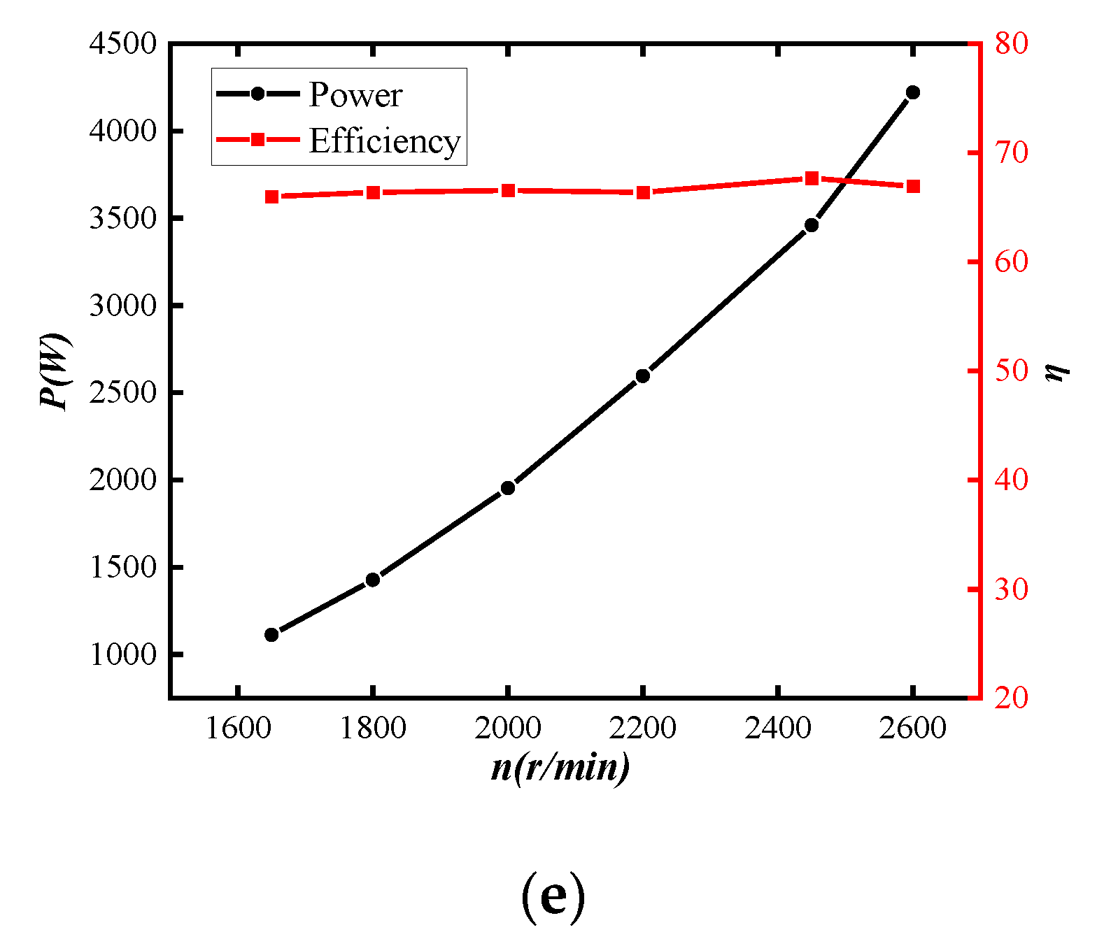
Figure 12e shows the power and efficiency (N-η) curve at different rotational speeds. The propulsion system shaft power along with the increase in speed shows a parabolic rise. The propeller efficiency remains unchanged (approximately 66%), indicating that the quasi-steady-state calculation process ignores the role of the rotational acceleration of the propeller impeller, and the transformation of energy is similar at different rotational speeds.

5.2. Hydrodynamic and Flow Field Characteristic Analysis of a Two-Pump Water Jet Propulsion Ship under Mooring Conditions

Under mooring conditions, the hydrodynamic characteristics of the water jet propulsion system at variable speeds were solved using non-constant numerical calculations. Similar patterns existed in the numerical predictions (Section 5.1), but there were also some differences, mainly in terms of the amplitude and curve jitter. Under mooring conditions, the rotating speeds of water jet propulsion ships are set at 1650, 1800, 2000, 2200 and 2450 r/min. The three working conditions, 1650, 2000, and 2450, were selected for flow field analysis.

Figure 13a shows the ship-pump head and flow rate curves at different rotational speeds. The pump head growth is parabolic with an increase in the rotational speed; as the speed increases, the system power increases, the work of the propeller blades on the water flow is enhanced, and the propeller energy loss is reduced. The head growth type is different and the system flow rate along with the increase in speed show linear growth, indicating that the water jet propeller at different speed holds a certain commonality.

Figure 13b shows the ship-pump torque thrust curves at different rotational speeds due to the energy difference between the pump inlet and outlet cross-sections of the fluid generating the system thrust. In this figure, the thrust force increases with the increase in the rotational speed, and its variation pattern is similar to the flow rate, which is positively correlated with the rotational speed in the working condition range. The system torque becomes larger as the rotational speed increases, indicating that the shaft power also increases.

Figure 13c shows the pressure variation curves of the inlet and outlet sections of the ship-pump propeller. Both the impeller inlet pressure and the guide vane outlet pressure increase continuously with the increase in the rotational speed, but the increase in the pressure in the impeller outlet section (approximately 10 kPa) is much larger than that in the impeller inlet section (approximately 5 kPa). This is because the power becomes larger as the rotational speed increases and the water flow also receives more energy. Therefore, the outlet pressure amplitude rises more rapidly. Comparing this curve to the one in Section 5.1, the magnitude of change is reduced, mainly due to the flow loss problem when the flow path and the hull bottom plate are matched.

Figure 13d shows the average velocity variation curves of the ship-pump variable speed propeller inlet and outlet sections. The velocities of both the inlet and outlet of the pump increase with the increase in the rotational speed, and the change of the outlet velocity (approximately 2.4 m/s) is larger than that of the inlet (approximately 1.2 m/s).

Figure 13e shows the N-η law of shaft power and propeller efficiency of the ship-pump system. The shaft power of the propulsion system shows a parabolic rise along with the increase in speed. However, the propeller efficiency remains the same (approximately 45%), indicating that the numerical prediction process ignores the role of the rotational acceleration of the propeller impeller. The conversion of energy is similar under different speed conditions. Meanwhile, the efficiency decreases under the open-water conditions in Section 5.1. Conversely, the efficiency is not high under the mooring condition; the flow loss when matching the propeller and the hull leads to a decrease in the propeller efficiency.

Figure 13f shows the ship-pump nozzle velocity curves for different rotational speeds. The nozzle velocity increases as the speed increases and is greater than the velocity at the exit of the guide vane cross-section. This is because the nozzle structure is similar to the compression pipe to maintain energy conservation, which makes the cross-sectional area smaller, and increases the average velocity of the cross-section.

The hydrodynamic characteristics analyzed in this subsection are compared with the results of the numerical prediction of the single pump in open water carried out in Section 5.1. Here, the water jet propellers are matched to the hull with the loss of runners, which affects the overall hydrodynamic performance of the ship. Therefore, the hydrodynamic performance parameters of the propellers matched on the ship model are reduced. This effect is evident under mooring conditions.

Figure 14 shows the comparison of the axial velocity distributions in the inlet channel of the propeller at different rotational speeds. The axial velocity of the inlet channel does not vary considerably with the rotational speed. However, from the general trend, there is a similar phenomenon as that of the axial velocity distribution in the mid-longitudinal section of the single pump in the open-water environment under mooring conditions in Section 5.1. The velocity in the area closer to the propulsion pump is larger. Moreover, the backflow phenomenon occurs in the lower edge of the flow channel, which is more significant in the water jet propulsion model in this section. The flow characteristics in the area below the propeller inlet are affected because the transition at the lip of the channel becomes less smooth when the channel is matched to the hull.

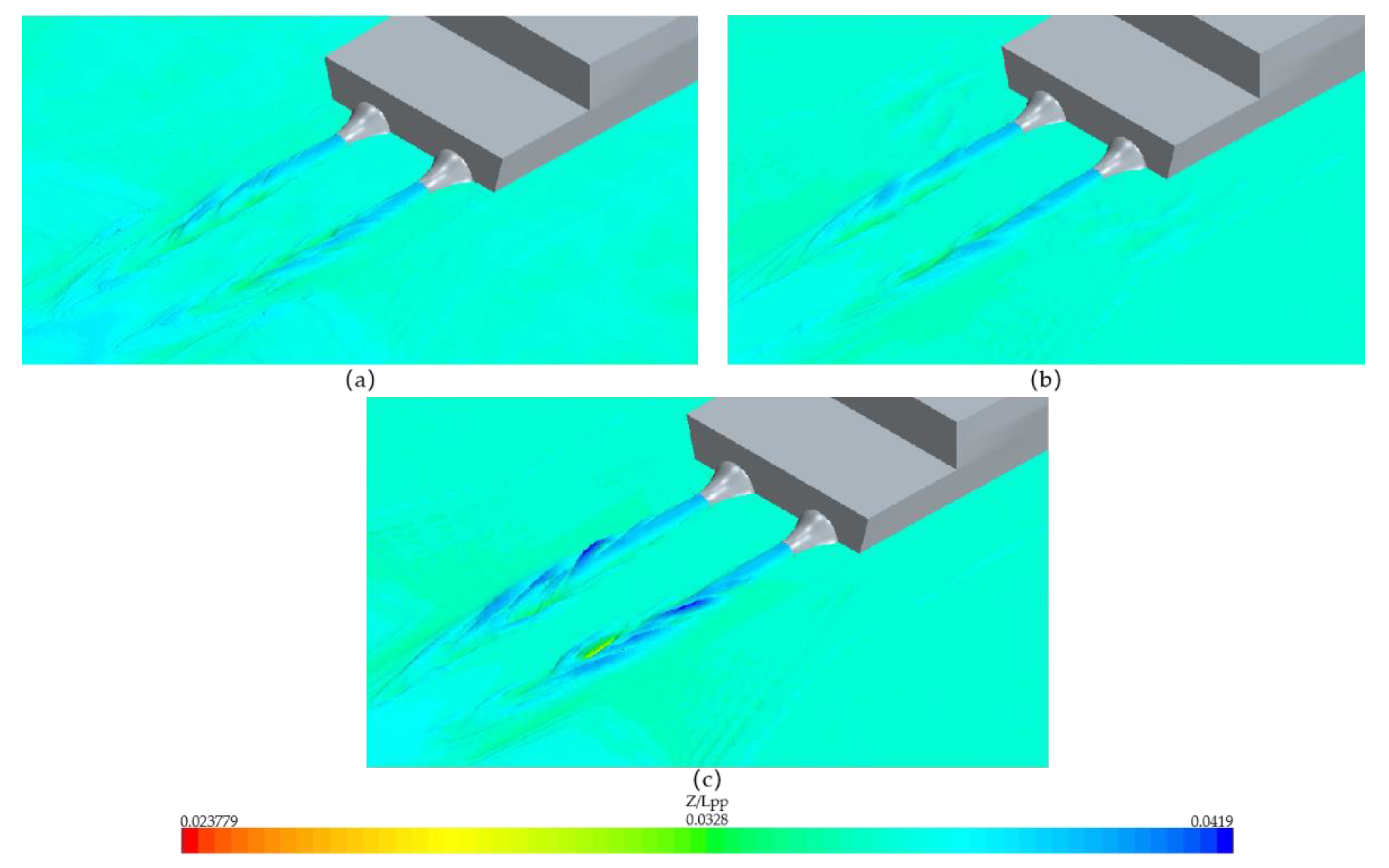
The disturbance phenomena of the nozzle jets of the variable rotational speed water jet propulsion ship model under mooring conditions are compared in Figure 15. The results show that, at lower rotational speeds (Figure 15a), a significant radial diffusion of the nozzle jet occurs in the closer region behind the ship model. The interactions between diffused and undiffused jets and between jets generated from different nozzles occur simultaneously. The starting positions of diffusion and disturbance start to move behind the stern plate as the rotational speed increases (Figure 15b,c). At the same time, with the enhancement of the interference, the characteristics of the free surface at the stern of the ship model become more complex. As the impeller speed increases, the force generated by the system increases accordingly, resulting in an increase in the flow rate through the flow channel and the nozzle jet head and energy, which causes the jet diffusion region to move backwards.

The turbulent kinetic energy distribution in the inlet disc surface (x/LPP = 0.0116) and the longitudinal section in the flow channel (y/LPP = 0.038) of the propeller were selected for the analysis of the flow field characteristics in the water jet propulsion ship.

In Figure 16, as the backflow phenomenon and propulsion shaft shading occur during mooring conditions, the high-speed position of the inlet disk is mainly in the upper disk, whereas the low-speed position is in the lower disk. Under mooring conditions, the unevenness of the axial velocity of the inlet disk surface of the propeller is significant. Simultaneously, the velocity variation of the inlet disk surface is distributed in the circumferential direction and the pump impeller area has a corresponding relationship.

Figure 17 presents the comparative analysis of the turbulent kinetic energy in the longitudinal section of the water jet propulsion system at different rotational speeds. The pipe contraction caused the turbulent kinetic energy to rise. Meanwhile, the axial velocity of the jet is still the main factor that influences energy. The pump area rotates the impeller to work on the fluid, and the flow field diameter and circumferential direction velocity components in the system change dramatically. The flow characteristics evolve while the turbulence is enhanced and the fluid flow is directed by the guide vane. The flow channel area is influenced by the inlet flow channel morphology, suction effect, and backflow effect under mooring conditions, and its flow form is dominated by the axial component while evolving along the fluid motion direction. The turbulent kinetic energy evolution of the flow field in the propeller is distributed in the regional flow separation locations.

In the numerical simulation, two monitoring points were set downstream on the inner object surface of the water jet propeller nozzle as P1 and P2, which are at an angle of 42° to the vertical surface (Figure 18). Two monitoring points were used to monitor the pulsating pressure upstream and downstream of the nozzle, calculating the flow rate at the nozzle using the differential pressure method.

The flow rate Q is expressed as

$$Q_{}=\sqrt{\frac{2(P_1-P_2)A_1^2{A}_2^2}{\rho (A_1^2-A_2^2)}},$$

(11)

where A₁ and A₂ are the overflow areas of the upper and lower sections of the propulsion pump nozzle, respectively, ρ is the fluid density, and P₁ and P₂ are the average pressure values of the flow field monitoring points at the upper and lower sections, respectively.

Table 10. Nozzle time domain pulsation pressure averages and flow data.

Rotational Speed (r/min)	1650	1800	2000	2200	2450
P1 (Pa)	6241.82	7295.33	8986.44	11,067.22	13,705.45
P2 (Pa)	3785.44	4512.39	5580.85	6798.18	8345.82
Q (m3/s)	0.01742	0.01853	0.02051	0.02296	0.02573

lists the average values of the time domain pulsation pressure obtained from the numerical prediction at different rotational speeds during the mooring condition. In addition, in this table, the flow rate through the water jet propeller at different rotational speeds calculated using Equation (8) is included. The flow rate plotted from the table is converted to mass flow rate, and the flow rate variation line graph is plotted (Figure 15a).

The results of the time domain pulsation pressure on the two measurement points at different speeds (i.e., 1650, 2000 and 2450 r/min) in the time domain are compared in Figure 19. As the rotational speed increases, the time domain pulsation pressure increases in the numerical prediction, while the time domain pulsation pressure curve at the measurement point P₁ is always above the measurement point P₂.

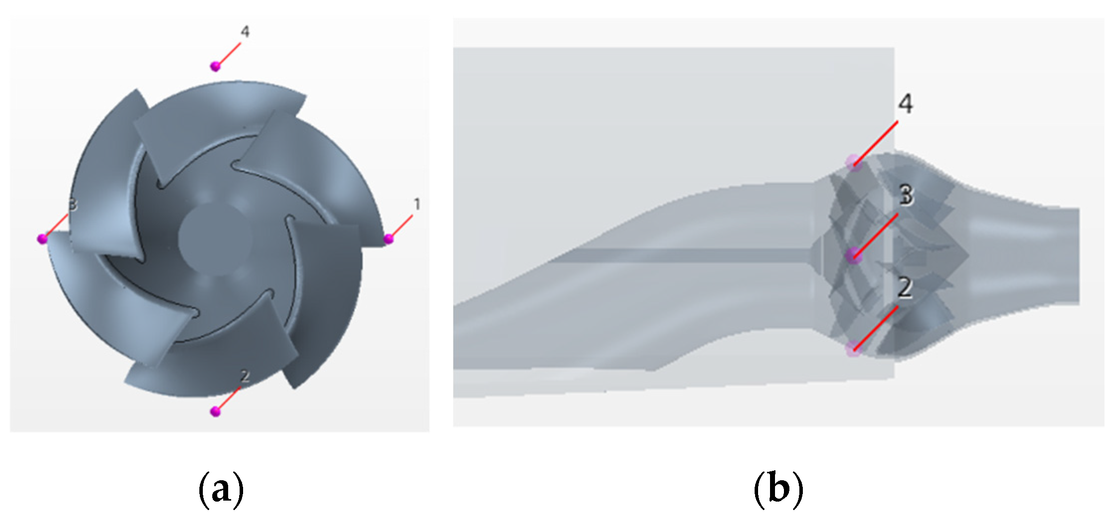
Monitoring points were set in the middle of the pump impeller and inlet channel model to monitor the pulsating pressure of the movement process. One monitoring point was set every 90° on the periphery of the impeller, numbered 1, 2, 3, and 4 in Figure 20.

Figure 21 shows the Fourier-transformed frequency domain pulsation pressure plots for the four monitoring points (1–4) at different rotational speeds under mooring conditions. Based on the figure, the first-order pulsation force amplitudes of monitoring points 2 and 4 are higher at the lower speed, as shown in Figure 20a. With an increase in the rotational speed, the first-order pulsation force amplitude at monitoring point 1 increases the most among the four points, while the change in pulsation force amplitude at monitoring point 3 is relatively less significant. Meanwhile, the pulsation force amplitude at monitoring point 3 does not change as significantly due to the flow channel loss that exists when the inlet channel and the hull are matched, which in turn leads to flow loss. Simultaneously, under mooring conditions, the backflow phenomenon also occurs at the lip of the flow channel, and the complex interaction between these two influences the pulsation pressure variation in the frequency domain at monitoring points 1 and 3. Generally, the higher the propulsion pump flow field inhomogeneity, the higher the frequency spectrum lobe frequency wave peak. As in the case of conventional propellers, the higher-order pulsation pressure amplitudes are all lower than that of the first-order one.

6. Conclusions

Fully discrete numerical prediction models, “water jet propulsion pump + inlet channel” and “hull + inlet channel + water jet propulsion”, were constructed based on the interfacing mesh method. The grid division was practical, the convergence efficiency and computational accuracy were high, the grid uncertainties were 1% and 2.4%, and the computational errors affected by the time step were 0.1% and 0.3%. Thus, the model is suitable for the study of hydrodynamic and flow field characteristics under mooring conditions.

The main conclusions of this study are as follows:

(1)

The analysis of the water jet propeller open-water field characteristics revealed that the suction effect of the impeller, the propulsion axis on the water flow obstruction effect, and mooring conditions that exist under the interaction of the backflow phenomenon affect the water jet propeller runner exit section and the axial velocity distribution in the longitudinal section, resulting in flow loss and the flow separation phenomenon on the lip. Conversely, from the pressure characteristic analysis, a subvelocity region around the exit section of the flow channel was identified, and the pressure changes at the pressure ramp and the lip angle in the middle longitudinal section are more apparent. The pressure minima of the inlet flow channel are mainly distributed at the lip angle, bend transition, and ramp.

(2)

The analysis of the hydrodynamic characteristics of the water jet propulsion model under mooring conditions shows that all parameters have different upward trends with the change in rotational speed. However, in comparison with the results of the single pump related forecasts, the parameters matched to the model have different degrees of decline due to the flow loss phenomenon when matching the water jet propulsion pump to the hull. The efficiency of the open-water jet propulsion pump is approximately 66% under mooring conditions and approximately 45% when matched to the water jet propulsion model.

(3)

The analysis of the internal flow field characteristics verifies that the pumping effect of the impeller and the backflow phenomenon interact to influence the turbulent kinetic energy distribution in the mid-longitudinal section of the water jet propeller.

References

1. Kandasamy, M.; Peri, D.; Tahara, Y.; Wilson, W.; Miozzi, M.; Georgiev, S.; Milanov, E.; Campana, E.F.; Stern, F. Simulation based design optimization of waterjet propelled Delft catamaran. Int. Shipbuild. Prog. 2013, 60, 277–308. [Google Scholar] [CrossRef]
2. Takai, T.; Kandasamy, M.; Stern, F. Verification and validation study of URANS simulations for an axial waterjet propelled large high-speed ship. J. Mar. Sci. Technol. 2011, 16, 434–447. [Google Scholar] [CrossRef]
3. Duerr, P.; von Ellenrieder, K.D. Scaling and Numerical Analysis of Nonuniform Waterjet Pump Inflows. IEEE J. Ocean. Eng. 2014, 40, 701–709. [Google Scholar] [CrossRef]
4. Yang, Q.; Wang, Y.; Zhang, Z. Numerical prediction of the fluctuating noise source of waterjet in full scale. J. Mar. Sci. Technol. 2014, 19, 510–527. [Google Scholar] [CrossRef]
5. Fung, S.; Karafiath, G.; Cusanelli, D.; McCallum, D.; JHSS. (Joint High-Speed Sealift Ship) Hull Form Development. Test and Evaluation. In Proceedings of the 9th International Conference on Fast Sea Transportation, Shanghai, China, 1 January 2007; p. FAST2007. [Google Scholar]
6. Liu, X.; Luo, J.; Liu, C. Analysis of water jet propeller hydrodynamic performance based on CFD. J. Phys. Conf. Ser. 2020, 1600, 012076. [Google Scholar] [CrossRef]
7. Jiang, F.; Li, Y.; Gong, J. Study on the manoeuvre characteristics of a trimaran under different layouts by water-jet self-propulsion model test. Appl. Ocean. Res. 2021, 108, 102550. [Google Scholar] [CrossRef]
8. Lefebvre, P.J.; Barker, W.P. Centrifugal Pump Performance During Transient Operation. J. Fluids Eng. 1995, 117, 123–128. [Google Scholar] [CrossRef]
9. Thanapandi, P.; Prasad, R. Centrifugal pump transient characteristics and analysis using the method of characteristics. Int. J. Mech. Sci. 1995, 37, 77–89. [Google Scholar] [CrossRef]
10. Thanapandi, P.; Prasad, R. A Quasi-Steady Performance Prediction Model for Dynamic Characteristics of a Volute Pump. Proc. Inst. Mech. Eng. Part A J. Power Energy 1994, 208, 47–58. [Google Scholar] [CrossRef]
11. Tsukamoto, H.; Matsunaga, S.; Yoneda, H.; Hata, S. Transient Characteristics of a Centrifugal Pump During Stopping Period. J. Fluids Eng. 1986, 108, 392–399. [Google Scholar] [CrossRef]
12. Tsukamoto, H.; Ohashi, H. Transient Characteristics of a Centrifugal Pump During Starting Period. J. Fluids Eng. 1982, 104, 6–13. [Google Scholar] [CrossRef]
13. Kandasamy, M.; Ooi, S.K.; Carrica, P.; Stern, F. Integral Force/Moment Waterjet Model for CFD Simulations. J. Fluids Eng. 2010, 132, 101103. [Google Scholar] [CrossRef]
14. Duplaa, S.; Coutier-Delgosha, O.; Dazin, A.; Roussette, O.; Bois, G.; Caignaert, G. Experimental Study of a Cavitating Centrifugal Pump During Fast Startups. J. Fluids Eng. 2010, 132, 021301. [Google Scholar] [CrossRef]
15. Duplaa, S.; Coutier-Delgosha, O.; Dazin, A.; Bois, G.; Caignaert, G. Experimental characterization and modelling of a cavitating centrifugal pump operating in fast start-up conditions. In Proceedings of the 13th International Symposium on Transport Phenomena and Dynamics of Rotating Machinery-ISROMAC-13, Honolulu, HI, USA, 4 April 2010. [Google Scholar]
16. Duplaa, S.; Coutier-Delgosha, O.; Dazin, A.; Bois, G.; Caignaert, G.; Roussette, O. Cavitation inception in fast startup. In Proceedings of the Twelfth International Symposium on Transport Phenomena and Dynamics of Rotating Machinery-ISROMAC-12, Honolulu, HI, USA, 17 February 2008. [Google Scholar]
17. Tanaka, T.; Tsukamoto, H. Transient Behavior of a Cavitating Centrifugal Pump at Rapid Change in Operating Conditions—Part 3: Classifications of Transient Phenomena. J. Fluids Eng. 1999, 121, 857–865. [Google Scholar] [CrossRef]
18. Chen, S.; Cheng, X.; Zhang, Y.; Ouyang, W. Application of Coanda Effect in Water Jet Propulsion Devices. J. Phys. Conf. Ser. 2021, 1846, 012095. [Google Scholar] [CrossRef]
19. Tanaka, T.; Tsukamoto, H. Transient Behavior of a Cavitating Centrifugal Pump at Rapid Change in Operating Conditions—Part 1: Transient Phenomena at Opening/Closure of Discharge Valve. J. Fluids Eng. 1999, 121, 841–849. [Google Scholar] [CrossRef]
20. Tanaka, T.; Tsukamoto, H. Transient Behavior of a Cavitating Centrifugal Pump at Rapid Change in Operating Conditions—Part 2: Transient Phenomena at Pump Startup/Shutdown. J. Fluids Eng. 1999, 121, 850–856. [Google Scholar] [CrossRef]
21. Zhang, X.; Hu, J.; Hong, B. Dynamic Response Computation of Single-Point Mooring of Product Tanker Based on AQWA. IOP Conf. Series Earth Environ. Sci. 2020, 527, 012010. [Google Scholar] [CrossRef]
22. Xu, S.W.; Liang, M.-X.; Wang, X.F.; Ding, A.-B. A Mooring System Deployment Design Methodology for Ships at Varying Water Depths. China Ocean Eng. 2020, 34, 185–197. [Google Scholar] [CrossRef]
23. Zhang, Y.; Zhu, Z.; Jin, Y.; Cui, B.; Li, Y.; Dou, H. Experimental study on a centrifugal pump with an open impeller during startup period. J. Therm. Sci. 2013, 22, 1–6. [Google Scholar] [CrossRef]
24. Li, Z.; Wu, P.; Wu, D.; Wang, L. Experimental and numerical study of transient flow in a centrifugal pump during startup. J. Mech. Sci. Technol. 2011, 25, 749–757. [Google Scholar] [CrossRef]
25. Anderson, J.D. Fundamentals of Computational Fluid Dynamics and Its Applications; Mechanical Industry Press: South Norwalk, CT, USA, 2007. [Google Scholar]
26. Rahman, M.M.; Vuorinen, V.; Taghinia, J.; Larmi, M. Wall-Distance-Free Formulation for SST k-ω model. Eur. J. Mech. B Fluids 2019, 75, 71–82. [Google Scholar] [CrossRef]
27. Carrier, A. Finite element implementation of k−ω SST with automatic wall treatment and adjoint-based mesh adaptation. Int. J. Numer. Methods Fluids 2020, 93, 703–719. [Google Scholar] [CrossRef]
28. Menter, F.R. Two-equation eddy-viscosity turbulence models for engineering applications. AIAA J. 1994, 32, 1598–1605. [Google Scholar] [CrossRef] [Green Version]
29. White, F.M. Fluid Mechanics, 4th ed.; McGraw-Hill Higher Education: New York, NY, USA, 1998. [Google Scholar]
Figure 1. Geometric model of the propulsion system.
Jmse 10 00953 g001
Figure 2. Propulsion pump computational domain division.
Jmse 10 00953 g002
Figure 3. Geometric model of the ship.
Jmse 10 00953 g003
Figure 4. Water jet propeller.
Jmse 10 00953 g004
Figure 5. Numerical calculation domain: (a) side view; (b) top view.
Jmse 10 00953 g005
Figure 6. Mesh refinement in the computation domain: (a) overall; (b) propeller mid-longitudinal section; (c) impeller; (d) guide leaf.
Jmse 10 00953 g006
Figure 7. Water jet propulsion pump inlet and outlet cross-section diagram.
Jmse 10 00953 g007
Figure 8. Inlet cross-sectional velocity of the propulsion pump at different rotational speeds: (a) 1650 r/min; (b) 2000 r/min; (c) 2450 r/min; (d) 2600 r/min.
Jmse 10 00953 g008
Figure 9. Inlet cross-sectional pressure of the propulsion pump at different rotational speeds: (a) 1650 r/min; (b) 2000 r/min; (c) 2450 r/min; (d) 2600 r/min.
Jmse 10 00953 g009
Figure 10. Axial velocity of the middle longitudinal profile at different rotational speeds: (a) 1650 r/min; (b) 2000 r/min; (c) 2450 r/min; (d) 2600 r/min.
Jmse 10 00953 g010
Figure 11. Pressure distribution in the middle and longitudinal profiles at different speeds: (a) 1650 r/min; (b) 2000 r/min; (c) 2450 r/min; (d) 2600 r/min.
Jmse 10 00953 g011
Figure 12. Hydrodynamic characteristic curve of the water jet propulsion system: (a) ship-pump head and flow rate (Q-H) variation curve; (b) ship-pump torque thrust (M-T) variation curve; (c) pressure change curve; (d) import and export speed change curve; (e) power and efficiency (N-η) curve.
Jmse 10 00953 g012aJmse 10 00953 g012b
Figure 13. Ship-pump system hydrodynamic curves: (a) ship-pump head and flow rate curves; (b) ship-pump torque thrust curves; (c) pressure variation curves of the inlet and outlet sections of the ship-pump propeller; (d) the average velocity variation curves of the ship-pump propeller inlet and outlet sections; (e) N-η law of shaft power and propeller efficiency of the ship-pump system; (f) ship-pump nozzle velocity curves.
Jmse 10 00953 g013aJmse 10 00953 g013b
Figure 14. Inlet flow channel around the flow field axial velocity distribution: (a) 1650 r/min; (b) 2000 r/min; (c) 2450 r/min.
Jmse 10 00953 g014
Figure 15. Jet morphology of the nozzle at different rotational speeds: (a) 1650 r/min; (b) 2000 r/min; (c) 2450 r/min.
Jmse 10 00953 g015
Figure 16. Axial velocity of water jet propeller inlet disc surface at different rotational speeds: (a) 1650 r/min; (b) 2000 r/min; (c) 2450 r/min.
Jmse 10 00953 g016
Figure 17. Turbulent kinetic energy distribution in the middle and longitudinal profiles: (a) 1650 r/min; (b) 2000 r/min; (c) 2450 r/min.
Jmse 10 00953 g017
Figure 18. Nozzle pressure monitoring point.
Jmse 10 00953 g018
Figure 19. Time domain pulsation pressure curves for different rotational speeds: (a) 1650 r/min; (b) 2000 r/min; (c) 2450 r/min. Note: the red line is P1 and the green line is P2.
Jmse 10 00953 g019
Figure 20. Schematic diagram of the location of the pulsation pressure monitoring point: (a) position of monitoring point relative to pump impeller; (b) position of monitoring point relative to flow channel.
Jmse 10 00953 g020
Figure 21. Histogram of pulsation force amplitude: (a) 1650 r/min; (b) 2000 r/min; (c) 2450 r/min.
Jmse 10 00953 g021aJmse 10 00953 g021b