On the Mechanism behind the Variation of the Tidal Current Asymmetry in Response to Reclamations in Lingding Bay, China

Abstract

Tidal current asymmetry, an important factor for waterborne substance transport, is strongly affected by the changing shoreline. Lingding Bay (LDB), located in the center of the Guangdong-Hong Kong-Macao Greater Bay Area, has suffered great shoreline changes since the 1970s. A well-validated numerical model is built to investigate how the changing shoreline impacts tidal current asymmetry, which is quantified by the skewness parameter. Two types of tidal current asymmetries, the flow velocity asymmetry (FVA) and the flow duration asymmetry (FDA), are considered here. Despite their different dominant combinations, the two asymmetries display a similar tendency from the mouth to the head of the LDB. When the shoreline changes due to successive land reclamation are taken into consideration, the FVA and the FDA alter correspondingly. The results suggest that the shoreline change shifts the FVA in Deep Bay (a side embayment of LDB) from ebb dominance to flood dominance, because of the changes of its dominant constituent combinations (K₁/O₁/M₂ and the residual current). As the shoreline propagates seaward, the increasing contributions of M₂/M₄ and M₂/S₂/MS₄ enlarge the water area of positive FDA (i.e., shorter duration of low water slack) in LDB. Analyses of tidal current asymmetries in Lingding Bay show that tidal current asymmetry has been enhanced by sustained land reclamation and will further impact sediment transport in the bay.

1. Introduction

Tidal asymmetry is one of the main factors that generates residual sediment transport [1] and is in relation to the migration of other waterborne substances, for instance, the contaminant [2]. Tidal asymmetry includes vertical and horizontal tidal asymmetries. It is generated not only by nonlinear tidal interactions in shallow water, but also by astronomical tides in the absence of shallow-water effects [3]. Boundary conditions and driving forces (e.g., runoff, sea level rise, atmosphere) are two of the main factors that affect tidal asymmetry [4].

In recent years, many deltas and estuaries are facing the threats from changing boundary conditions, caused by human activities: (1) dredging for depth increase or maintenance [5,6,7,8], sand mining [9,10,11], and changed bathymetry; (2) land reclamation [12,13,14,15], hydraulic structures [16,17], changed surface area, and shoreline. To understand the implications of these variable factors in the estuaries, much research has been developed worldwide.

Water depth exerts a strong influence on tides. The extensive dredging impacts the tidal amplitude and phase positively or negatively [5,7,8]. In addition, the sand mining deepens the down cutting depth, removes the tidal flat and changes the bed roughness, e.g., in the San Francisco Bay [10]. Moreover, it enhances the tidal range and tidal amplitude and seasonally increases the persistence of mobile mud [11]. These would have influence on the waterworks for domestic, industrial, farming purposes, and navigation.

The shoreline change affects the tides as well and its importance for the changing tides was commented on by Hoitink [18]. Shoreline change, due to human interventions, exceeds that caused by the natural factors and brings pronounced impact on the tides. The hydraulic structures would change the tidal characteristics at the project area. For example, the tidal power station, in the Rance Estuary, France, switched the dominance of flood/ebb in the estuary [17]. The coastal constructions even impact the tides in far-field water areas, e.g., in the western coast of Korea [16].

Compared with hydraulic structures, land reclamation changes the shoreline on a larger scale. Reclamations are often carried out by coastal cities in order to satisfy the land need for human survival and development. The interaction between the reclamation and the tides in adjacent seas can produce irregular water-level variations [14] or differences in tidal asymmetry [19,20,21]. Large-scale reclamations could also cause far-field impacts [22]. Moreover, the changing hydrodynamic conditions would induce variations in the transport of sediment, salt, and other waterborne substances and affect the ecological environment [13,23,24]. For example, the transport of fine sediment responds to the changes of current velocity with a time lag [3]. The probabilities of plastic debris presence are higher for positive asymmetric tides than for symmetric or negative asymmetric tides [25].

Most of the previous studies focused on the duration asymmetry in tidal elevation, and the studies on the tidal current were less and limited by stations [26,27,28]. This is because the data on tidal levels is much easier to obtain than the tidal current data. However, the tidal current asymmetry, mainly including the flow velocity asymmetry (FVA) and the flow duration asymmetry (FDA), plays the more decisive role in waterborne substance transport [29]. Furthermore, it is more sensitive to the variations in external forcing and river morphology [30].

The Pearl River Estuary, located in the center of the Guangdong-Hong Kong-Macao Greater Bay Area, China, suffers rapid urbanizing and fast-growing land requirement. Large-scale land reclamations have been constructed since the 1970s, and resulted in tidal flat area reduction, especially in Lingding Bay (LDB). For instance, about 21.2 km² of land reclamation has happened along the northern coastline of the Deep Bay (the side embayment of the LDB) from 1986 to 2007 and reduced 14% of the original water surface area of the bay [23]. Large scale land reclamation affects the coastal hydrodynamic conditions by changing the shoreline [21]. The main objectives of this paper are to illustrate the characteristics of the tidal current asymmetries in LDB and to find out their responses to the shoreline change caused by successive land reclamations. The skewness parameter is introduced instead of the traditional method to quantify the tidal current asymmetry and to distinguish the contributions of different combinations of tidal constituents.

This paper is arranged as follows. The next section is a brief introduction on the study area, the model, and the analysis methods. Section 3 presents the spatio-temporal distribution of the main tides and the asymmetries. Section 4 discusses the intrinsic mechanism of the asymmetries and its response to the shoreline change. Finally, our conclusions are presented in Section 5.

2. Materials and Methods

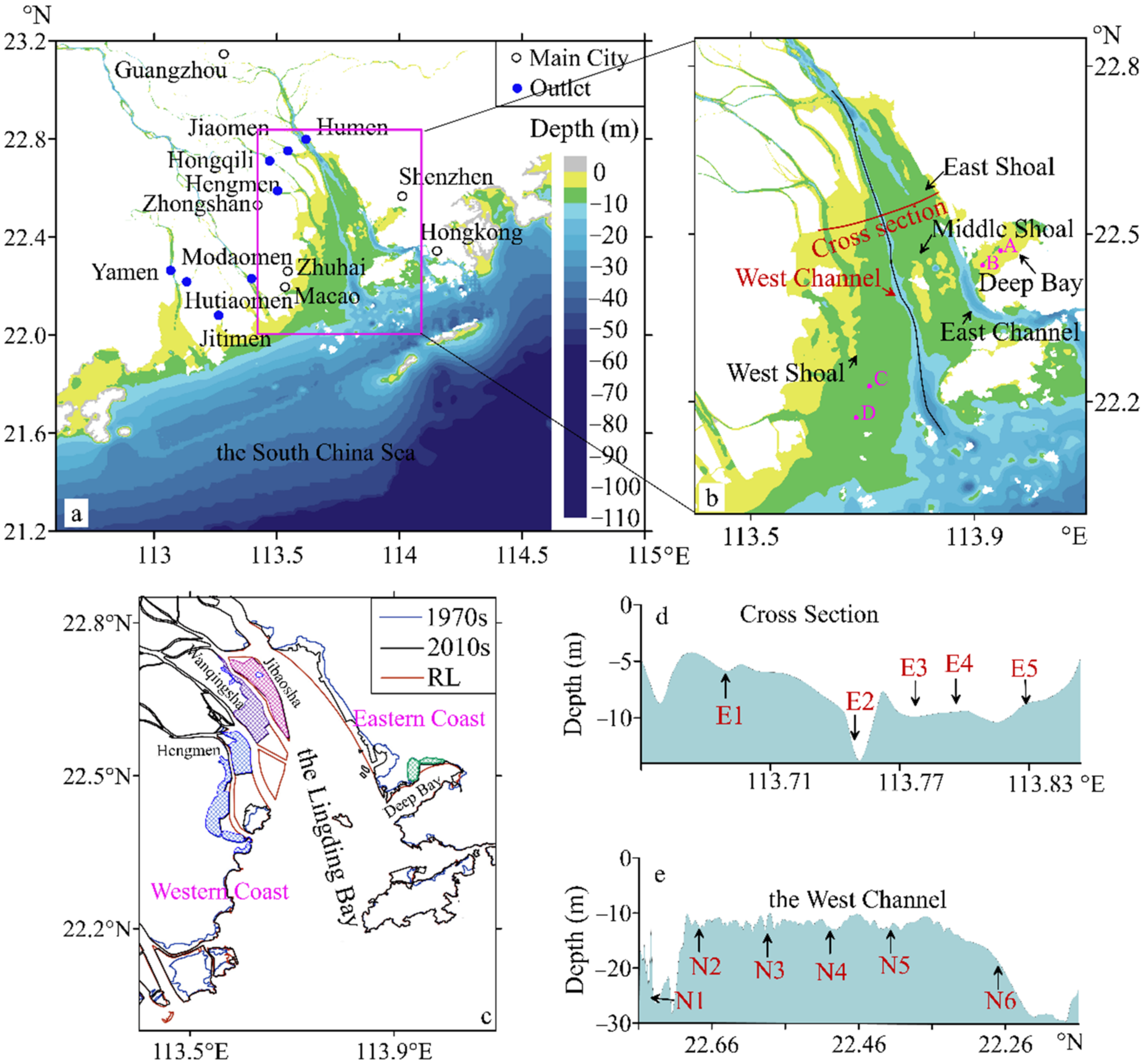
2.1. Setting and Shoreline Change

The Pearl River is the second largest river in China in terms of the discharge, which amounts to 3 × 10¹¹ m³/yr of water and 8 × 10⁶ t/yr of sediment [31]. About 40% of the total suspended sediment was transported into Lingding Bay (LDB) [32]. LDB, a large estuary of the Pearl River, includes the eastern four outlets, namely, Humen (tide-dominated), Jiaomen, Hongqili, and Hengmen (Figure 1a). Lingding Bay has a convergent geometry. The topography is split into three shoals by the East and West Channels, and the shoals are named the West, the Middle, and the East Shoals, respectively (Figure 1b). The channels are the main ways for navigation to and from the ports, with the depth of over 5 m on average [33].

LDB has a mixed semi-diurnal tidal system with an average tidal range of 1.0–1.7 m [34]. The M₂ is the most important astronomical tide, followed by S₂, K₁, O₁. The tidal current is mainly reciprocating flow. The influence of the summer monsoon is so strong that only 20% of annual precipitation and 20% of the discharge from the Pearl River happens in the dry season [35,36]. Thus, the dry season is chosen as the study period to minimize the influence of other forces (e.g., runoff).

To satisfy the needs of the land, large-scale reclamation has taken place in LDB, and the water areas have decreased by 2.67 billion square meters since the 1970s (Figure 1c) [37]. The reclamation activities straightened the shoreline and extended it seaward by about 580 m on the average [38]. In the rapidly developing years, the extending speed of the shoreline in LDB even exceeded 100 m/a [33,39], which is much faster than those in the Yangtze River (20 m/a) and the Yellow River (48 m/a) [39]. Significant changes can be found along the western coast of LDB and Deep Bay (Figure 1c).

However, land reclamation is a double-edged sword, which also creates a negative influence on the ecosystem and humans’ daily life sometimes. Hence, from the 2010s, the Pearl River Water Resources Commission of the Ministry of Water Resource carries out a regulation [40] and delimits the reclamation within the regulation line (RL), as shown in Figure 1c. Since then, the rate of land reclamation has slowed down. However, this activity still exists and its effect on tides is on a long timescale [4].

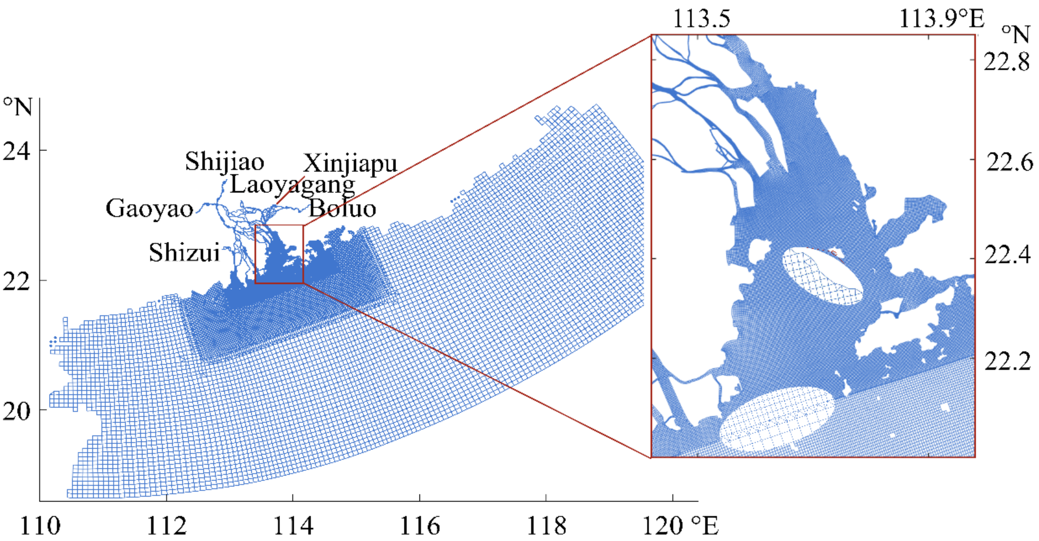
2.2. Hydrodynamic Model

A 2D hydrodynamic model based on Delft3D Flow Flexible Mesh is applied to examine hydrodynamic conditions of the study area [41,42]. The large-scale domain is situated between longitudes 110.2° E and 120.4° E, and latitudes 18.7° N and 24.7° N, covering the entire river networks and estuaries of the Pearl River and the northern South China Sea (Figure 2). A mesh of unstructured quadrilateral or triangular elements was generated with the model grid size ranging from 50 m to 50 km. The topological data include the field data of the river networks from 2010, nautical charts of LDB from 2015 published by the Maritime Safety Administration of China, and the ETOPO1 Global Relief Model [43] for the inner shelf region. The model is driven by the predicted tidal level obtained from the TPXO8 global model of ocean tides [44], and the measured daily discharges at Gaoyao, Shijiao, Boluo, Laoyagang, Shizui, and Xinjiapu stations (positions shown in Figure 2). The monthly average discharges increased from about 2400 m³ to 3000 m³ during our study period, from 1 January 2005 to 1 April 2005. The roughness ranges from 0.008 to 0.037, with an increasing tendency from the estuary to the river networks.

The time steps are self-regulated according to the CFL condition. The start time step is 1 s and the maximum time step is 30 s. All simulations are run for 90 days, of which the last 75 days are used for harmonic analysis to obtain the amplitudes of each constituent of the tidal currents, and their respective phases. It is a barotropic model where the salinity and temperature are set to be constant.

Three scenarios of model experiments are conducted to reproduce and study the impacts of land reclamation. In the first scenario, the model is run with the shoreline of the 1970s, which is the era during which large-scale reclamation had not been started yet. The shoreline of the 2010s is used in the second scenario. It is set as the basic scenario, representing the shoreline after significant reclamations between the 1970s and the 2010s. The shoreline of the third scenario is updated into the regulation line (RL), which is the extreme scenario that the reclamation project reaches the regulation line. To simplify the uncertain factors in estimating the evolution of the tidal current, the same hydrodynamic boundaries and bathymetry are used in the three scenarios.

2.3. Quantification Method of the Tidal Asymmetry

During the last decades, three kinds of methods are mainly used to quantify tidal asymmetry: (1) harmonic method [45], the most traditional one, which is based on the phase difference and amplitude ratio of the interacting tidal constituents; (2) probability distribution functions [46]; and (3) skewness [47]. The first method requires identifying the dominant contributive constituent. It will be difficult to compare the asymmetries at different locations since the asymmetries involve different constituent combinations. The second method is hampered when a large number of constituents are considered. By contrast, the skewness method can be used on any time series with different dominant constituents. It can be used in more complex situations when several different combinations contribute to the overall asymmetry simultaneously [48]. Thus, the skewness method is more suitable for this study region.

2.3.1. The Total Skewness

The total skewness of flow velocity asymmetry (FVA) and the flow duration asymmetry (FDA) are estimated, using the following formula [47]:

$$\gamma \left(x\right)=\frac{\frac{1}{\mathrm{N}-1}{{\displaystyle \sum }}_{i=1}^{\mathrm{N}}{\left(x_i-\overline{x}\right)}^3}{{\left[\frac{1}{\mathrm{N}-1}{{\displaystyle \sum }}_{i=1}^{\mathrm{N}}{\left(x_i-\overline{x}\right)}^2\right]}^{3/2}}$$

(1)

where γ is skewness; x_i is the time series of sample signals; $\overline{x}$ is the mean value of the samples; and N is the number of equal distanced (hourly) time series data. When x denotes the velocity, the calculated skewness quantifies the FVA; for x denoting the acceleration of tidal current velocity, the skewness quantifies the FDA. A positive γ means a flood dominance for FVA (${\gamma }_{FVA}>0$) and a shorter duration of low water slack for FDA (${\gamma }_{FDA}>0$) and vice versa. The direction of positive velocity is defined as perpendicular with the bay mouth and along the flood tide direction, as most of the current in the LDB is in the northwest-southeast direction [35]. The larger the skewness is, the more asymmetric the tidal current is.

2.3.2. The Main Tidal Combination Skewness

The skewness of the different combinations of tidal constituents are calculated by Equations (2) and (3) [49]:

For FVA:

$${\gamma }_{CFVA}=\frac{{{\displaystyle \sum }}_{{\omega }_i+{\omega }_j={\omega }_k}\frac{3}{2}{a}_i{a}_j{a}_{k}cos\left({\phi }_i+{\phi }_j-{\phi }_k\right)+{{\displaystyle \sum }}_{2{\omega }_i={\omega }_j}\frac{3}{4}{a}_i^2{a}_{j}cos\left(2{\phi }_i-{\phi }_j\right)+{{\displaystyle \sum }}_{i=1}\frac{3}{2}{a}_i^2{a}_{0}cos\left({\phi }_0\right)+a_0^{3}cos\left({\phi }_0\right)}{{\left(a_0^2+\frac{1}{2}{{\displaystyle \sum }}_{i=1}^N{a}_i^2{\omega }_i^2\right)}^{3/2}}$$

(2)

For FDA:

$${\gamma }_{CFDA}=\frac{{{\displaystyle \sum }}_{{\omega }_i+{\omega }_j={\omega }_k}\frac{3}{2}{a}_i{\omega }_i{a}_j{\omega }_j{a}_k{\omega }_{k}sin\left({\phi }_i+{\phi }_j-{\phi }_k\right)+{{\displaystyle \sum }}_{2{\omega }_i={\omega }_j}\frac{3}{4}{a}_i^2{\omega }_i^2{a}_j{\omega }_{j}sin\left(2{\phi }_i-{\phi }_j\right)}{{\left(\frac{1}{2}{{\displaystyle \sum }}_{i=1}^N{a}_i^2{\omega }_i^2\right)}^{3/2}}$$

(3)

where $a_i$, ${\phi }_i$ and ${\omega }_i$ are the amplitude, phase, and frequency of the corresponding tidal constituent, respectively, gained from the harmonic analysis on the time series of velocity; $a_0$ is the amplitude of the Eulerian flow velocities, equaling to the average velocity over the 73 full tidal periods; and ${\phi }_0$ is the direction of the residual current. In this study, the residual current is simply obtained as the mean velocity in the running window (25 h) period. A positive residual flow has a zero phase, whereas a negative one has a 180° phase. Furthermore, the skewness is computed using a moving window (25 h) to capture subtidal change and the duration variation. Through these equations, the contributions of different tidal combinations can be distinguished and compared clearly.

The modeled current velocities are analyzed into 35 harmonic constituents by performing a classical harmonic analysis with nodal corrections, using the MATLAB version of T-Tide [50]. In total, 20 constituents were judged to be significant, on average. However, only combinations of two or three constituents meeting the frequency condition $2{\omega }_i={\omega }_j$ or ${\omega }_i+{\omega }_j={\omega }_k$, contribute to long-term asymmetry. Song et al. [51] found that the combinations of M₂/M₄ and M₂/S₂/MS₄ were dominant in semidiurnal regimes, whereas K₁/O₁/M₂ and P₁/K₁/S₂ dominated the diurnal and mixed, but mainly diurnal regimes. Zhang et al. [52] and Gong et al. [49] had the common thought that K₁/O₁/M₂, M₂/M₄, M₂/S₂/MS₄ contributed most to tidal asymmetry in the Pearl River Estuary. Thus, the six main constituents (M₂, S₂, K₁, O₁, M₄, MS₄) are finally selected to calculate the asymmetries and explain the intrinsic mechanisms of the FVA and FDA.

3. Results

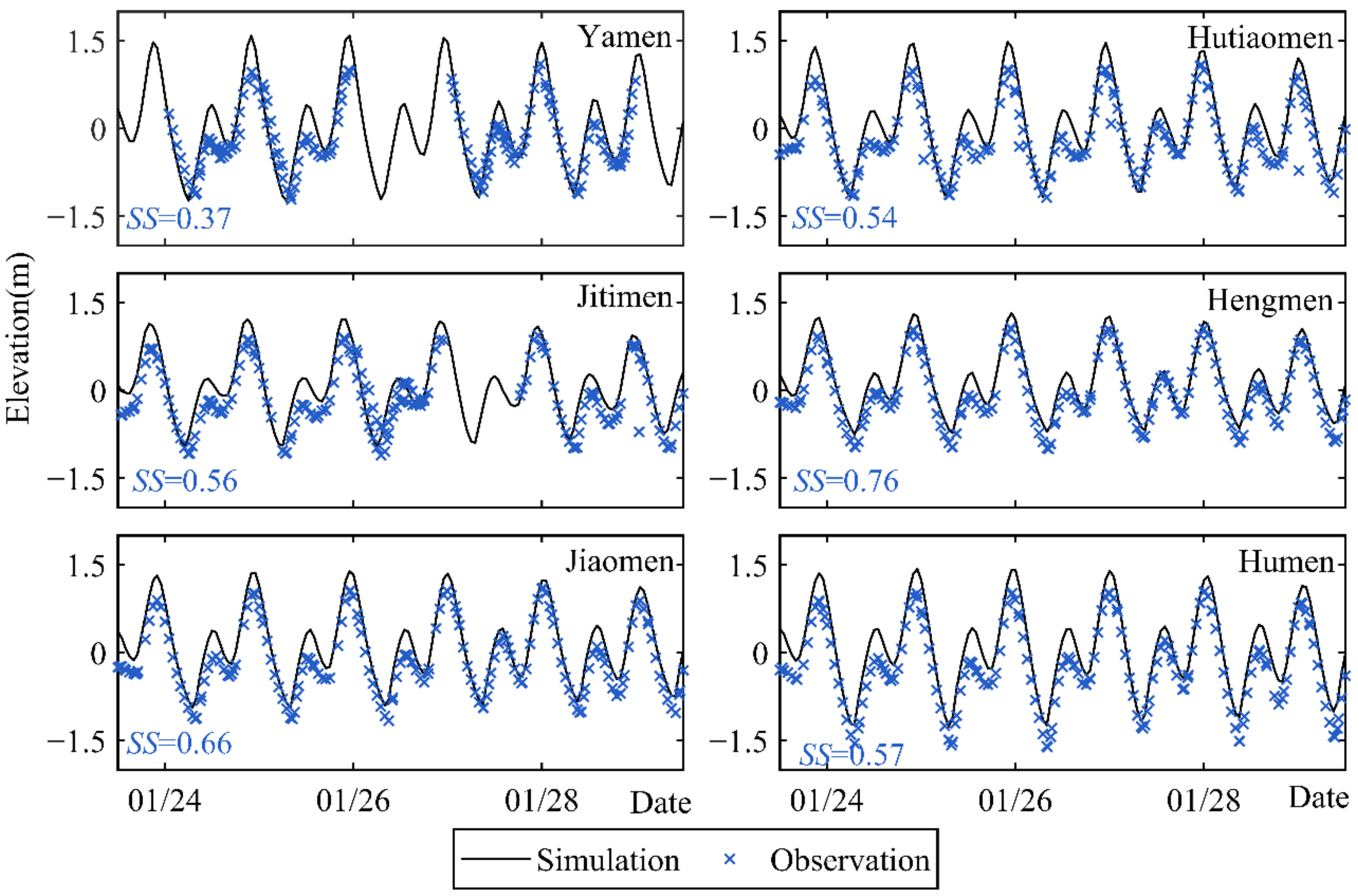
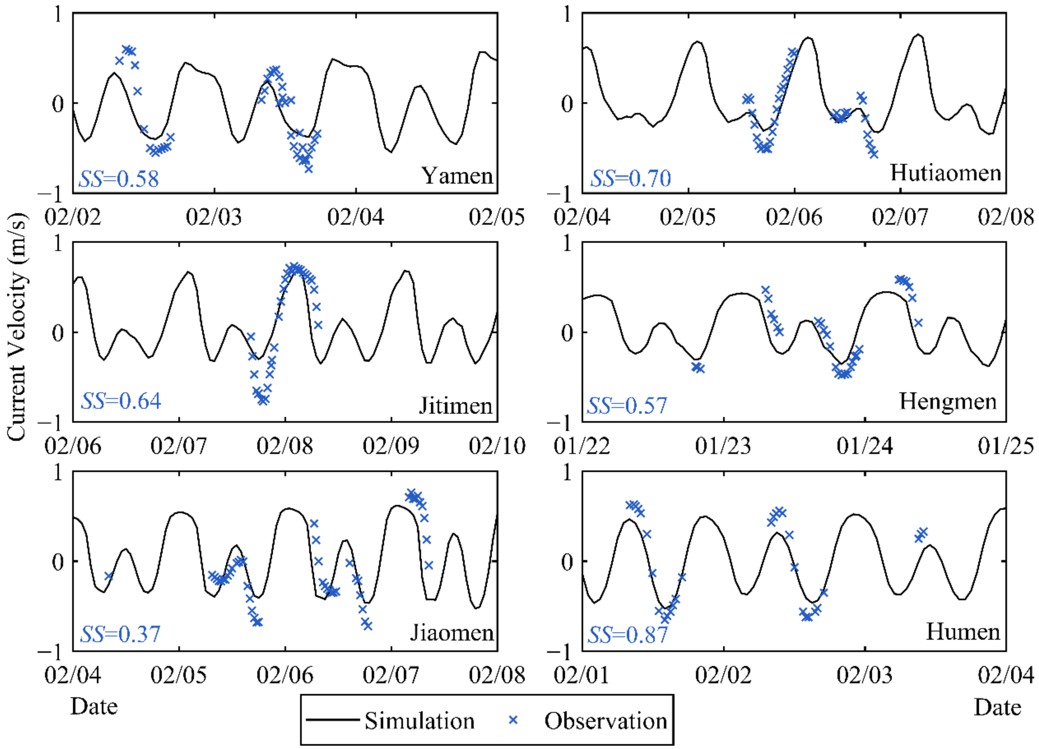
3.1. Model Performance Evaluation

Water surface elevations and current velocities recorded at six coastal tidal stations (positions shown in Figure 1a) are taken into calibrations. The simulated tidal levels from 12:00 noon on 1/23/2005 to 12:00 noon on 1/29/2005 are selected to compare with the field data (Figure 3). The validation of simulated tidal current data has been taken with the corresponding data (Figure 4). The results prove that the model captures the tidal elevations and the tidal current velocities well, which are supported by the skill score (SS), calculated by Equation (4) [53].

$$SS=1-\frac{\sum {\left(X_{obs}-X_{mod}\right)}^2}{\sum {\left(X_{obs}-{\overline{X}}_{obs}\right)}^2}$$

(4)

where $X_{obs}$ and $X_{mod}$ are the observed values and modeled values of the water elevation or current velocity. The performance levels of SS are categorized as: >0.65 excellent; 0.65–0.5 very good; 0.5–0.2 good; <0.2 poor [53]. Both tidal levels and currents are highly correlated to the field data with most SS over 0.5, which are regarded as very good performance. Additionally, the few small SS of the currents is still above the acceptable level (SS > 0.2). Consequently, the model results reflect good agreement with the observed values, with acceptable errors.

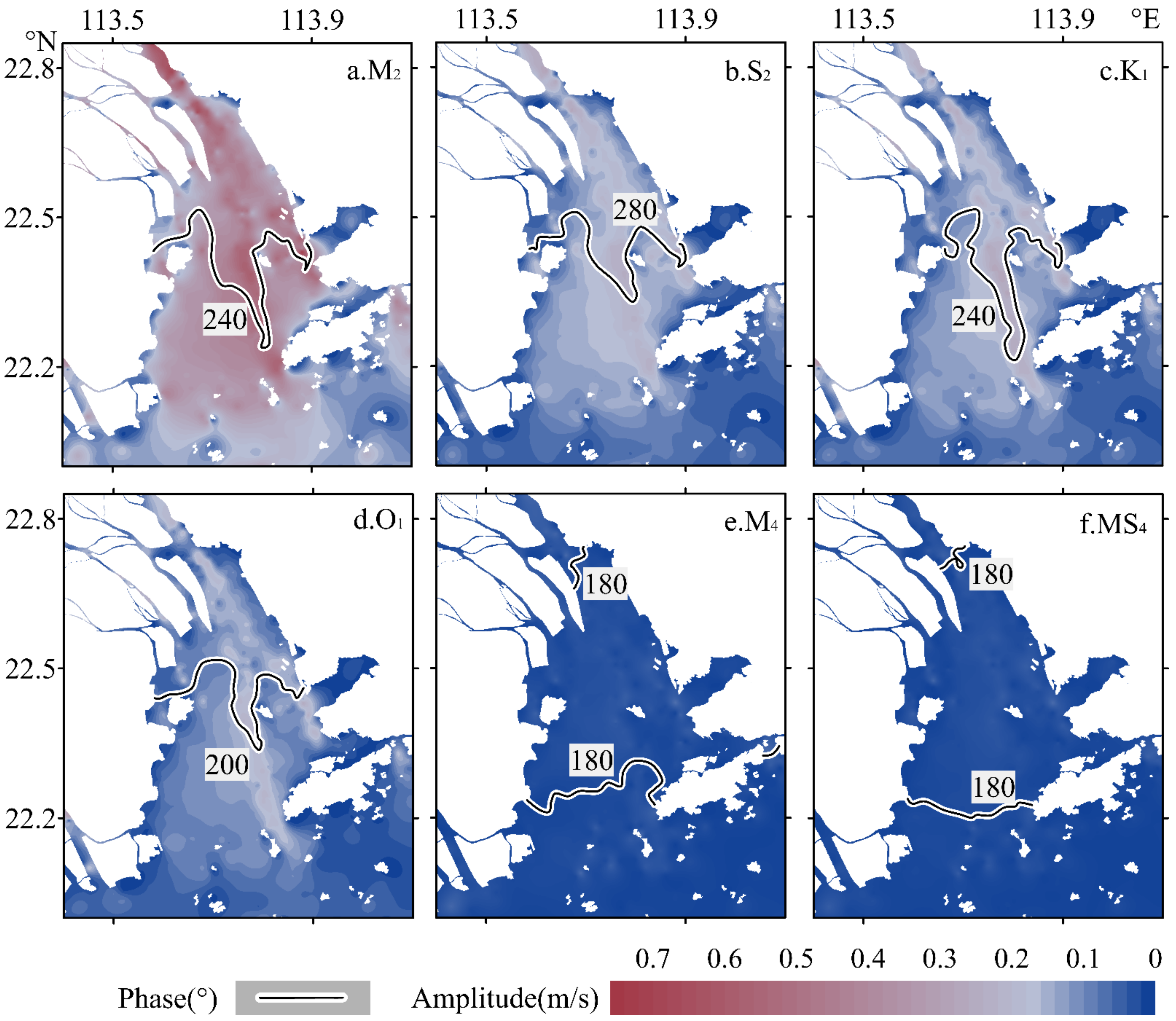
3.2. The Spatial Variation of Tidal Current Constituents

After the harmonic analysis of the tidal currents, constituents M₂, S₂, K₁, O₁, M₄, MS₄ are selected as the main constituents. According to the form factor (F = $(a_{O_1}+a_{K_1}$)/($a_{M_2}+a_{S_2}$)) of the current velocities, the values between 0.25–1.5 indicate that the currents in LDB are mainly mixed, but dominantly semi-diurnal [54]. The dominant astronomical tide is M₂, followed by S₂, K₁ and O₁. The major shallow water tides are M₄ and MS₄. As shown in the Figure 5, the amplitudes of the astronomical tides increase when entering LDB, due to the convergence of shoreline. The amplitudes of M₄ and MS₄ are obviously smaller than these of the astronomical tides. In this section, the spatial distribution of the amplitudes and phases of the selected tidal are demonstrated.

It can be seen from Figure 5a that M₂ is the dominant semi-diurnal tidal constituent, which is consistent with the conclusion of Mao et al. [28]. The current amplitudes of M₂ varies from 0.2 m/s along the adjacent sea area to about 0.4 m/s on average in the Lingding Bay. The amplitudes in the channels are larger than those on the shoals and the maximum value (1.25 m/s) occurs in the West Channel. The current phases are different between the channels and the shoals with the pronounced lags in the channels.

The amplitude distribution of K₁, O_1, and S₂ are similar (Figure 5b–d). In the adjacent sea area, the average amplitudes are about 0.05 m/s, then grow up to 0.1 m/s~0.4 m/s in LDB. Lower friction means higher flow rates in the channels. The amplitudes of K₁ and O₁ in the channels are about 0.1 m/s larger than those on the shoals, and for the S₂, it is 0.05 m/s. The phases of O₁ may deviate up to 40° from K₁ and 80° from S₂. Compared with the O₁ and S₂, the phases of K₁ show a farther lag, especially in the West Channel since it is the main ebb channel.

Although the current amplitudes of M₄ and MS₄ (Figure 5e,f) are smaller than these of the astronomical tides, they play a dominant role in flow duration asymmetry [49]. In the adjacent sea area, the amplitudes are about 0.009 m/s on average. As the estuary becomes narrower and shallower, the energy of the tides is concentrated. Then, advection effects induce the energy transfer from the astronomical tides to the shallow water tides. Finally, the amplitudes increase to 0.03 m/s near the Humen outlet. However, the increasing tendency of the phases is fluctuant because of the energy dissipation induced by the friction. Different from the monotonical increase of the astronomical tidal phases, the phases of M₄ and MS₄ are about 300° in the adjacent sea area, then rapidly decrease towards the middle and gradually increase to 180° towards the head of Lingding Bay.

3.3. The Spatio-Temporal Distribution of Asymmetry

Here, we analyze the spatio-temporal variations of tidal current asymmetries via the gamma parameter proposed by Nidzieko [47], which combines amplitude ratio and relative phase into one parameter. The tidal current velocities and their accelerations are used to compute the total skewness of flow velocity asymmetry (FVA) and flow duration asymmetry (FDA), respectively. The time series of each skewness are analyzed to detect the variation in the research period. Figure 6 and Figure 7 show the spatio-temporal distribution of the asymmetries. It should be noticed that the x axes in the Figure 6b,c and Figure 7b,c represent the number of the full tidal period (~25 h).

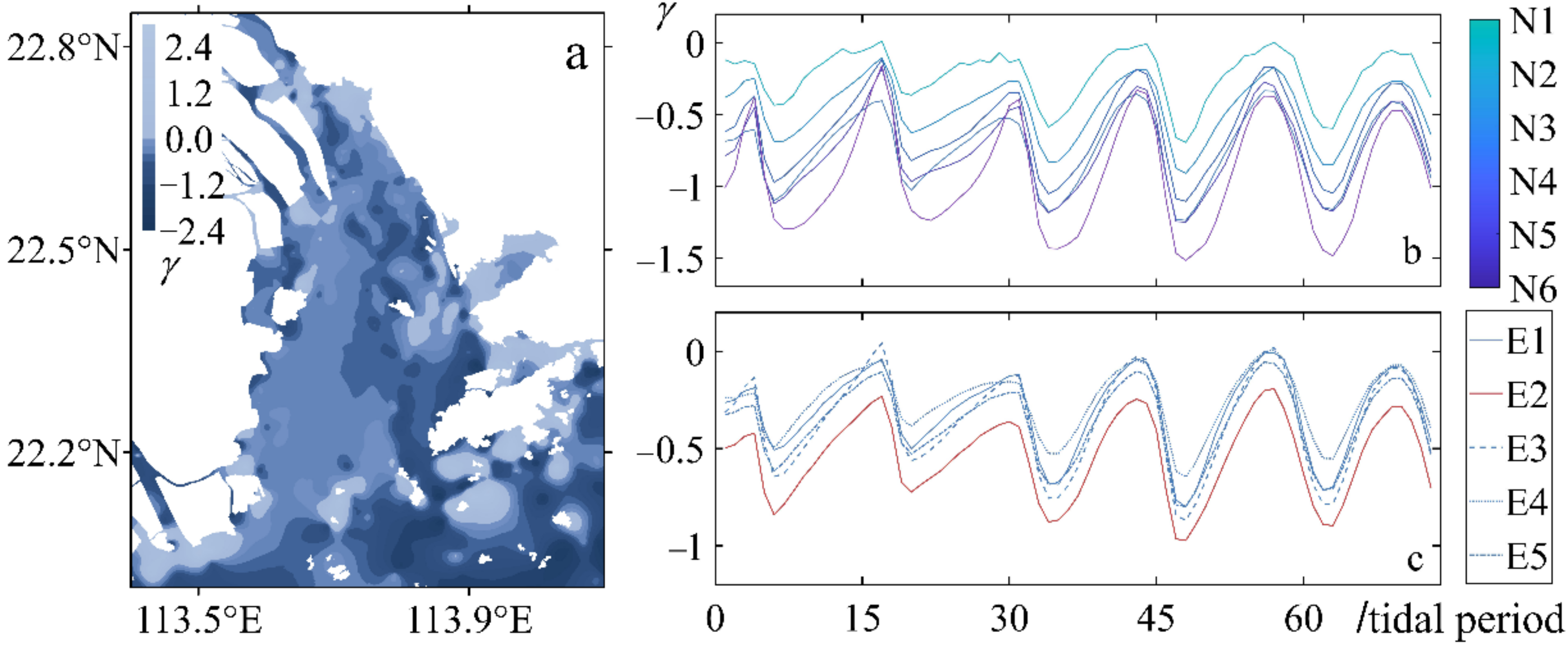
3.3.1. Flow Velocity Asymmetry (FVA)

Most of the FVA in Lingding Bay is ebb dominance with negative skewness (Figure 6a). It means that the peak ebb current velocity is higher than the peak flood current velocity. In LDB, a noticeable variation happens between the shoals and the channels, providing the average skewness of about −0.3 and −0.55, respectively. It demonstrates that the water depth is one of the factors affecting the flow velocity asymmetry. Another main factor is the convergent shoreline, which is reflected by the decreasing values and ranges of the skewness from the station N6 to N1 (Figure 6b). In the adjacent sea area, the FVA is also ebb dominance and even more asymmetric. This would be explained by the intrinsic mechanisms in Section 4.1. Moreover, the flood dominance appears in the areas with complex bathymetry, e.g., near the islands.

In order to verify the variation of the FVA, time series curves of the total skewness of the selected stations are performed (Figure 6b,c). During the study period, the stations are ebb dominance all the time. The skewness of these stations is in a regular fortnight cycle and the values reach the peaks at the same time. The increasing amplitudes of the skewness suggest an intensification of ebb dominance condition with time. The reason for the increase should probably be attributed to the raising river discharge, which enhances the ebb dominance through enlarging the ebb current.

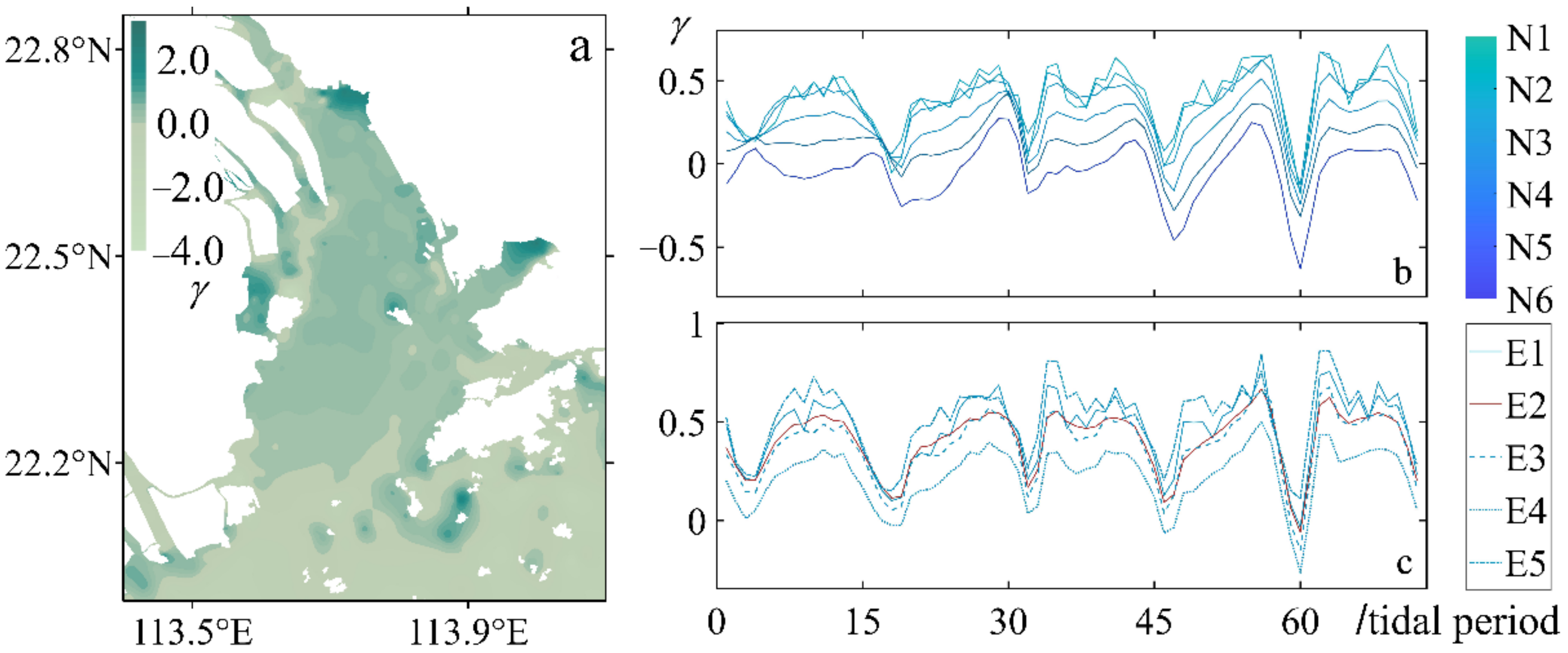
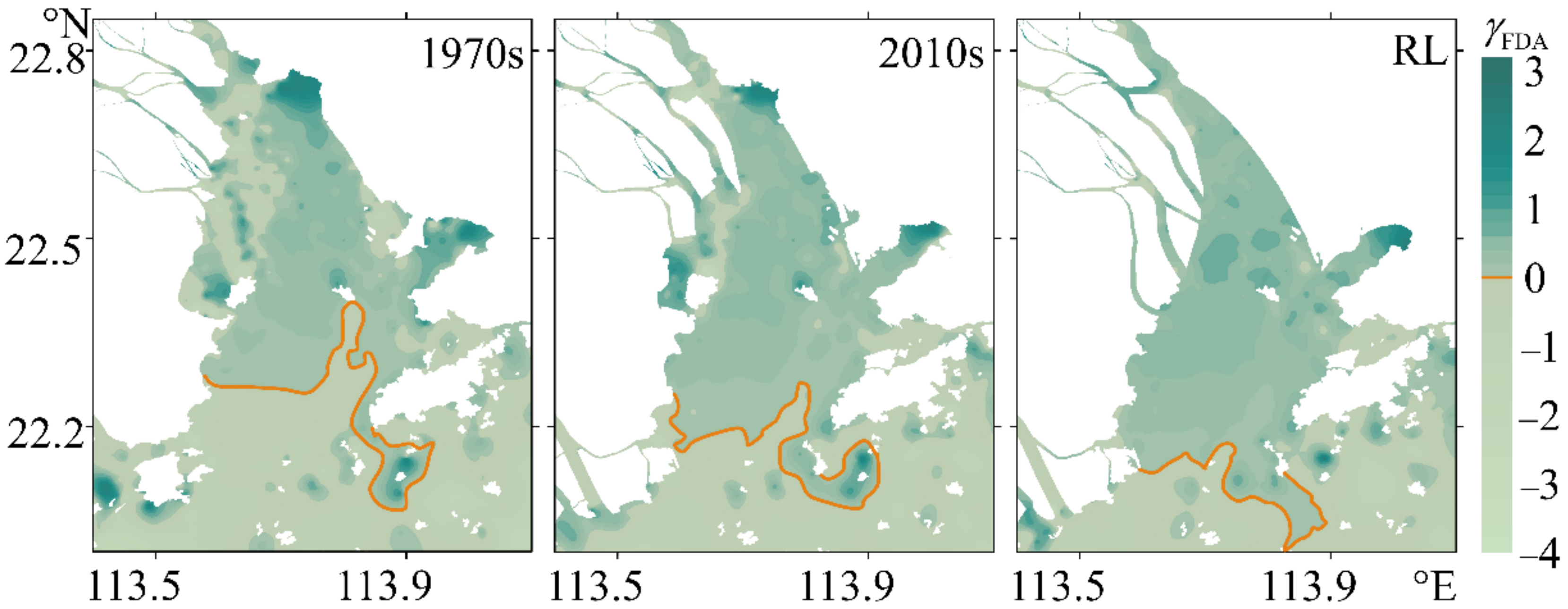
3.3.2. Flow Duration Asymmetry (FDA)

The flow duration asymmetry is pronounced during the survey period. As shown in Figure 7a, in the adjacent sea area, the skewness is negative. Subsequently, it switches from negative to positive at the bay mouth (near the station N6), and gradually increases to 0.5 along the upstream direction. In most parts of Lingding Bay, the skewness of the FDA is positive and about 0.4 on average. It indicates a shorter duration of low water slack. Then the skewness decreases at the head of the bay rapidly. Extreme values happen at the edges of shoreline and islands.

Time series of the FDA are shown in Figure 7b,c. The FDA of all stations, which is also in a 14-day period, reaches peak values at the same time and is in advance of the FVA. This can be explained from the physical relationship between the calculated data, the flow velocity (for FVA) and the acceleration of flow velocity (for FDA). Time series of the skewness of most stations show as positive during the study period except station N6, which is located at the bay mouth. Additionally, the positive peak skewness of the cycles tends to increase with time, probably due to the influence of river runoff.

In short, the FVA is sensitive to shoreline convergence and water depth, whereas the FDA is more sensitive to the convergence of the shoreline and the runoff. Lingding Bay is in a process with the shorter duration of low water slack (FDA > 0) and the higher ebb flow velocity (FVA < 0) (dry season). This will change the direction and the speed of the waterborne substance transport and will help to flush the sediment of LDB, moreover, which will change the morphological evolution of the estuary.

4. Discussions

4.1. Asymmetry from Principal Tidal Constituents

Skewness can not only be used to quantify and compare the asymmetries of tidal current records at different stations, regardless of the tidal regime (diurnal, mixed, semi-diurnal) or the constituents that dominate the asymmetry, but also measure the net effects of multiple tidal interactions, which possibly augment or reduce each other in creating net tidal asymmetry. Thus, the individual skewness from the different combinations of tidal constituents are shown in Figure 8. Different combinations of the mainly tidal constituents (K₁/O₁/M₂, M₂/M₄, M₂/S₂/MS₄ and residual current) are calculated by Equations (2) and (3). Although there are slight differences between the total skewness and the sum skewness of the main combinations, they are not significant enough to comment on further.

For the FVA, the K₁/O₁/M₂ triad makes a negative contribution and takes a large part (Figure 8a), which is due to the larger tidal amplitudes than those of the shallow water tides. Therefore, under the domination of K₁/O₁/M₂, the duration curves of the FVA (Figure 6b,c) are smoother than those of the FDA (Figure 7b,c). The ${\gamma }_{{\mathrm{K}}_1/{\mathrm{O}}_1/{\mathrm{M}}_2}$ demonstrates an increase at first (from the station N6 to N5), then a gradual decrease to station N1. This is synchronistical with the change of phase difference. For the FDA (Figure 8b), the K₁/O₁/M₂ only dominates in the adjacent sea area (outside of the station N6), prior to any internal distortions within the estuary. Then, the ${\gamma }_{{\mathrm{K}}_1/{\mathrm{O}}_1/{\mathrm{M}}_2}$ of FDA decreases from station N6 to N1. The reason for the decrease of ${\gamma }_{{\mathrm{K}}_1/{\mathrm{O}}_1/{\mathrm{M}}_2}$, either for the FVA or FDA, is the increasing energy transport from the astronomical tides to the shallow water tides. This energy transport behaves more pronounced on the FDA.

Because of the small amplitudes of M₄ and MS₄, their contributions to the FVA are minor (Figure 8a). Although their skewness exists, because of sharp changes between the stations N2 and N3, the ebb dominance cannot be reversed. However, the components M₂/M₄ and M₂/S₂/MS₄ play dominant roles for the FDA, more important than the K₁/O₁/M₂ triad (Figure 8b). Their skewness is larger due to their high frequencies. Similar to the distribution of the phases of M₄ and MS₄ (Figure 5e,f), the skewness of M₂/M₄ and M₂/S₂/MS₄ appears as a fluctuant increase along the upstream direction. In contrast with that of the FVA, the FDA induced by the shallow water tides is more asymmetric in the channel.

The residual current is equally important as K₁/O₁/M₂ for FVA (Figure 8a). Though the amplitudes of the residual current are relatively small, they induce considerable skewness by interacting with the tidal constituents. From stations N6 to N1, the contribution of residual current demonstrates a decreasing tendency in general. The difference between stations N4 and N3 can be explained by the suddenly narrowed estuary. Furthermore, the significant distinction in the cross section (E1~E5) shows that the contribution of residual current to FVA is strongly affected by the water depth.

4.2. Effect of the Shoreline Change on the FVA

The spatial distribution pattern of FVA in the LDB remains similar, although the shoreline is changing (Figure 9). All scenarios demonstrate a predominant tendency of ebb dominance, and preform the pronounced difference between the channels and shoals. However, the differences between scenarios are limited except in some local areas, for instance, the western coast and Deep Bay. Along the western coast, the positive skewness region shrank with the land reclamation of the tidal flat from the 1970s to the 2010s, then nearly disappears in the RL scenario. Moreover, the skewness shows a different tendency in Deep Bay. The skewness of the FVA changes from negative to positive gradually, from the 1970s to the RL (Figure 9). It means the tidal current in this area is in the tendency switching from ebb dominance to flood dominance, which favors net landward sediment transport [29]. Zhang and Mao argued that human activities in Deep Bay aggravated the severe sediment deposition further [55], which agrees well with our findings here.

In order to ascertain the influence of the shoreline changes in Deep Bay on asymmetry and the intrinsic mechanism, the points A and B (positions shown in the Figure 1b) have been selected for comparison (

Table 1. Comparison of tidal harmonic parameters in different scenarios at points A and B.

		A			B
		1970s	2010s	RL	1970s	2010s	RL
	${\gamma }_{FVA}$	−0.233	0.021	0.048	−0.047	0.151	0.261
	${\gamma }_{{\mathrm{K}}_1/{\mathrm{O}}_1/{\mathrm{M}}_2}$	−0.297	−0.252	−0.231	−0.248	−0.212	−0.202
Skewness	${\gamma }_{{\mathrm{M}}_2/{\mathrm{M}}_4}$	0.000	0.062	0.118	0.051	0.083	0.139
	${\gamma }_{{\mathrm{M}}_2/{\mathrm{S}}_2/{\mathrm{MS}}_4}$	0.000	0.049	0.081	0.049	0.071	0.108
	${\gamma }_{residual}$	−0.183	0.004	−0.043	0.059	0.164	0.163
	$a_{{\mathrm{O}}_1}\left(\mathrm{m}/\mathrm{s}\right)$	0.084	0.064	0.057	0.057	0.049	0.044
	$a_{{\mathrm{K}}_1}\left(\mathrm{m}/\mathrm{s}\right)$	0.102	0.079	0.070	0.069	0.061	0.057
Amplitude	$a_{{\mathrm{M}}_2}\left(\mathrm{m}/\mathrm{s}\right)$	0.268	0.224	0.206	0.200	0.191	0.177
	$a_{{\mathrm{S}}_2}\left(\mathrm{m}/\mathrm{s}\right)$	0.111	0.099	0.093	0.087	0.086	0.081
	$a_{{\mathrm{M}}_4}\left(\mathrm{m}/\mathrm{s}\right)$	0.017	0.024	0.029	0.022	0.021	0.025
	$a_{{\mathrm{MS}}_4}\left(\mathrm{m}/\mathrm{s}\right)$	0.019	0.019	0.022	0.018	0.016	0.019
	$a_{residual}\left(\mathrm{m}/\mathrm{s}\right)$	−0.014	0.000	−0.003	0.003	0.009	0.008
	${\phi }_{{\mathrm{O}}_1}+{\phi }_{{\mathrm{K}}_1}-{\phi }_{{\mathrm{M}}_2}\left(°\right)$	184.12	181.98	184.20	184.61	181.65	179.82
Relative phase	$2{\phi }_{{\mathrm{M}}_2}-{\phi }_{{\mathrm{M}}_4}\left(°\right)$	89.94	62.52	48.16	68.17	53.58	38.86
	${\phi }_{{\mathrm{M}}_2}+{\phi }_{{\mathrm{S}}_2}-{\phi }_{{\mathrm{MS}}_4}\left(°\right)$	89.99	58.54	47.65	60.67	42.61	32.36

). The skewness changes, between the 1970s and the 2010s, are generally larger than those between the 2010s and the RL scenarios. As previously suggested, the combinations M₂/M₄ and M₂/S₂/MS₄ are in favor of a positive skewness whereas K₁/O₁/M₂ contributes to a negative value, normally. Negative asymmetry is attenuated by the decreasing of the astronomical tide amplitudes and the increasing shallow water tides, as well as by the positive residual current. Finally, the flow velocity asymmetry in Deep Bay changes from negative to positive, followed by the transport direction change of the coarse sediment.

The negative values of the FVA demonstrate the ebb dominance, favoring the seaward transport of coarse sediment [29]. This is of benefit for keeping the channel depth in LDB. However, the positive asymmetry in Deep Bay will cause a sediment infill especially in periods of small river discharge and the continued increasing skewness will enhance it, e.g., in the RL scenario.

4.3. Effect of the Shoreline Change on the FDA

Corresponding to each scenario, the locations of the main contour line (${\gamma }_{FDA}$ = 0) of the FDA are compared in Figure 10. Significant shrinking of the negative area is observed along the western coast due to the land reclamation. The positive area has an obviously seaward extension: about 4 km, from the 1970s to the 2010s scenarios; and about 1.5 km between the 2010s and the RL scenarios. These changes would alter the deposition location of fine sediment. Meanwhile, there is an increase in the average skewness from 0.3 (in the 1970s) to 0.4 (in the 2010s), then to 0.5 (in the RL). It means that the stronger the convergence, the more ascendant the low water slack. In addition, the positive value of the FDA favors the landward transport of fine sediment [29].

To determine the impacts of the shoreline changes on the asymmetry and the intrinsic mechanism near the bay mouth, the points C and D (locations shown in the Figure 1b) have been selected for comparison (

Table 2. Comparison of tidal harmonic parameters in different scenarios at points C and D.

		C			D
		1970s	2010s	RL	1970s	2010s	RL
	${\gamma }_{FDA}$	−0.090	0.078 (+187%)	0.272 (+248%)	−0.311	−0.143 (+54%)	0.066 (+146%)
Skewness	${\gamma }_{{\mathrm{K}}_1/{\mathrm{O}}_1/{\mathrm{M}}_2}$	−0.010	−0.011 (−1%)	−0.015 (−6%)	−0.022	−0.025 (−1%)	−0.032 (−5%)
	${\gamma }_{{\mathrm{M}}_2/{\mathrm{M}}_4}$	−0.044	0.022 (+73%)	0.100 (+100%)	−0.130	−0.059 (+23%)	0.030 (+62%)
	${\gamma }_{{\mathrm{M}}_2/{\mathrm{S}}_2/{\mathrm{MS}}_4}$	0.046	0.058 (+13%)	0.086 (+36%)	−0.006	0.006 (+4%)	0.037 (+22%)
	$a_{{\mathrm{O}}_1}\left(\mathrm{m}/\mathrm{s}\right)$	0.109	0.094	0.083	0.094	0.083	0.073
	$a_{{\mathrm{K}}_1}\left(\mathrm{m}/\mathrm{s}\right)$	0.137	0.120	0.107	0.121	0.108	0.095
	$a_{{\mathrm{M}}_2}\left(\mathrm{m}/\mathrm{s}\right)$	0.353	0.326	0.290	0.298	0.279	0.249
Amplitude	$a_{{\mathrm{S}}_2}\left(\mathrm{m}/\mathrm{s}\right)$	0.136	0.129	0.116	0.111	0.107	0.096
	$a_{{\mathrm{M}}_4}\left(\mathrm{m}/\mathrm{s}\right)$	0.007	0.002	0.011	0.016	0.007	0.003
	$a_{{\mathrm{MS}}_4}\left(\mathrm{m}/\mathrm{s}\right)$	0.009	0.007	0.010	0.008	0.005	0.004
	${\phi }_{{\mathrm{O}}_1}+{\phi }_{{\mathrm{K}}_1}-{\phi }_{{\mathrm{M}}_2}\left(°\right)$	186.28	187.48	190.93	192.96	195.88	201.20
Relative phase	$2{\phi }_{{\mathrm{M}}_2}-{\phi }_{{\mathrm{M}}_4}\left(°\right)$	225.81	66.82	60.65	232.77	225.10	122.56
	${\phi }_{{\mathrm{M}}_2}+{\phi }_{{\mathrm{S}}_2}-{\phi }_{{\mathrm{MS}}_4}\left(°\right)$	134.38	100.72	71.14	184.77	172.31	106.72

The values in the bracket are calculated by $\left({\gamma }_{i+1}-{\gamma }_i\right){/}_{FDAi}$, where $i$ corresponds the scenarios respectively, e ${\gamma }_i$ is the related skewness, ${\gamma }_{FDAi}$ is the total skewness of the corresponding scenario.

). The asymmetry induced by the K₁/O₁/M₂ triad is ebb dominance in each scenario and is in an increasing tendency with the shoreline change, although their amplitudes decrease. It demonstrates that the relative phase change affects ${\gamma }_{{\mathrm{M}}_2/{\mathrm{S}}_2/{\mathrm{MS}}_4}$ more than the amplitude change. The shoreline change alters the sign of the asymmetries induced by the shallow water tides and the dominant constituents. As the relative phase of the M₂/M₄ and M₂/S₂/MS₄ combinations changing from 180°~360° to 0°~180°, the skewness of the FDA changes from negative to positive.

Comparing the three scenarios, it can be found that the combination of M₂/M₄ is the most sensitive in the FDA to the shoreline change, with variations of 23–100%. Meanwhile, the amplification of ${\gamma }_{{\mathrm{M}}_2/{\mathrm{S}}_2/{\mathrm{MS}}_4}$ is also obviously larger than that of ${\gamma }_{{\mathrm{K}}_1/{\mathrm{O}}_1/{\mathrm{M}}_2}$. Thus, there is an obvious effect of the shoreline change on the total FDA dominated by the shallow water tides.

In other words, the variations indicate that under the shoreline change, the source area of fine sediment for landward transport will be wider and the transport will be stronger. This might affect the position of the estuarine turbidity maximum (ETM) and the levels of oxygen concentration even further, impair the optimal functioning of estuarine ecosystems, and have multiple environmental and societal implications [56].

5. Conclusions

This study examines characteristics of the tidal current asymmetries in Lingding Bay under the rapid shoreline change due to large-scale reclamation using a numerical model. We mainly consider two asymmetries, the flow velocity asymmetry (FVA) and flow duration asymmetry (FDA). Three kinds of shoreline corresponding to different reclamation epochs are set into simulations, respectively, and the tidal current asymmetries are quantified by skewness.

Simulations reveal that tidal current asymmetry performs higher ebb velocity and longer ebb duration in LDB. Changes in tidal current asymmetries are spatially nonuniform and often amplified toward the head of the estuary. It means that the asymmetries are strongly related to the shape of the estuary. The FVA is made dominant by the astronomical tides and the residual current; thus, the effect of water depth on the FVA is also pronounced. The combinations of M₂/M₄ and M₂/S₂/MS₄ overcome the K₁/O₁/M₂ triad at the bay mouth and gradually increase into the dominant contributors in the FDA.

Both the FVA and FDA are sensitive to shoreline change. For instance, the variation of FVA happens in the Deep Bay; with the shoreline change, the increasing asymmetry induced by the shallow water tides and the changing residual current offset the negative asymmetry caused by the combination K₁/O₁/M₂. This change in FVA led to the deposition in Deep Bay, which is in the negative impact for the navigation and the water depth keeping here. The seaward extending of the symmetrical line (skewness = 0) in the FDA changes the deposition position of fine sediment, which will affect both navigation and the ecosystem. The FDA is more sensitive to the shoreline change than the FVA due to the different dominant contributors.

It is noted that the tempo-spatial distribution of tidal current asymmetries is important for substance transport, not only the sediment but also the contaminants and the plastics. The results of this study enrich our understanding of the variations in tidal current asymmetries in response to human reclamation, which could be of practical significance to estuary management in maintaining navigation channels and conserving the ecological environment.

References

1. Brown, J.M.; Davies, A.G. Flood/ebb tidal asymmetry in a shallow sandy estuary and the impact on net sand transport. Geomorphology 2010, 114, 431–439. [Google Scholar] [CrossRef]
2. Mao, X.; Enot, P.; Barry, D.A.; Li, L.; Binley, A.; Jeng, D.-S. Tidal influence on behaviour of a coastal aquifer adjacent to a low-relief estuary. J. Hydrol. 2006, 327, 110–127. [Google Scholar] [CrossRef]
3. Hoitink, A.J.F.; Hoekstra, P.; van Maren, D.S. Flow asymmetry associated with astronomical tides: Implications for the residual transport of sediment. J. Geophys. Res. 2003, 108, 3315. [Google Scholar] [CrossRef]
4. Talke, S.A.; Jay, D.A. Changing tides: The role of natural and anthropogenic factors. Annual Reviews of Marine Science. Annu. Rev. Mar. Sci. 2020, 12, 121–151. [Google Scholar] [CrossRef] [PubMed] [Green Version]
5. Bolle, A.; Wang, Z.B.; Amos, C.; De Ronde, J. The influence of changes in tidal asymmetry on residual sediment transport in the Western Scheldt. Cont. Shelf Res. 2010, 30, 871–882. [Google Scholar] [CrossRef]
6. Vellinga, N.E.; Hoitink, A.J.F.; van der Vegt, M.; Zhang, W.; Hoekstra, P. Human impacts on tides overwhelm the effect of sea level rise on extreme water levels in the Rhine-Meuse delta. Coast. Eng. 2014, 90, 40–50. [Google Scholar] [CrossRef]
7. van Maren, D.S.; van Kessel, T.; Cronin, K.; Sittoni, L. The impact of channel deepening and dredging on estuarine sediment concentration. Cont. Shelf Res. 2015, 95, 1–14. [Google Scholar] [CrossRef] [Green Version]
8. Talke, S.A.; Familkhalili, R.; Jay, D.A. The influence of channel deepening on tides, river discharge effects, and storm surge. J. Geophys. Res. Ocean. 2021, 126, e2020JC016328. [Google Scholar] [CrossRef]
9. Luo, X.-L.; Zeng, E.-Y.; Ji, R.-Y.; Wang, C.-P. Effects of in-channel sand excavation on the hydrology of the Pearl River Delta, China. J. Hydrol. 2007, 343, 230–239. [Google Scholar] [CrossRef]
10. Barnard, P.L.; Erikson, L.H.; Kvitek, R.G. Small-scale sediment transport patterns and bedform morphodynamics: New insights from high-resolution multibeam bathymetry. Geo-Mar. Lett. 2011, 31, 227–236. [Google Scholar] [CrossRef]
11. Jalon-Rojas, I.; Sottolichio, A.; Hanquiez, V.; Fort, A.; Schmidt, S. To what extent multidecadal changes in morphology and fluvial discharge impact tide in a convergent (turbid) tidal river. J. Geophys. Res. Ocean. 2018, 123, 3241–3258. [Google Scholar] [CrossRef]
12. Pelling, H.E.; Uehara, K.; Green, J.A.M. The impact of rapid coastline changes and sea level rise on the tides in the Bohai Sea, China. J. Geophys. Res. Ocean. 2013, 118, 3462–3472. [Google Scholar] [CrossRef] [Green Version]
13. Talke, S.A.; Kemp, A.C.; Woodruff, J. Relative sea level, tides, and extreme water levels in Boston harbor from 1825 to 2018. J. Geophys. Res. Ocean. 2018, 123, 3895–3914. [Google Scholar] [CrossRef]
14. Cao, D.; Shen, Y.; Su, M.; Yu, C. Numerical simulation of hydrodynamic environment effects of the reclamation project of Nanhui tidal flat in Yangtze Estuary. J. Hydrodyn. 2019, 31, 603–613. [Google Scholar] [CrossRef]
15. Qian, P.; Feng, X.; Feng, W.; Zhang, W. Response of tidal asymmetry to coastline changes in radial sand ridges sea area. Hydro-Sci. Eng. 2020, 3, 51–60. (In Chinese) [Google Scholar]
16. Suh, S.W.; Lee, H.W.; Kim, H.J. Spatio-temporal variability of tidal asymmetry due to multiple coastal constructions along the west coast of Korea. Estuar. Coast. Shelf Sci. 2014, 151, 336–346. [Google Scholar] [CrossRef]
17. Rtimi, R.; Sottolichio, A.; Tassi, P. Tidal Patterns and Sediment Dynamics in a Hypertidal Estuary Influenced by a Tidal Power Station. J. Coast. Res. 2020, 95, 1520–1524. [Google Scholar] [CrossRef]
18. Hoitink, A.J.F. Comment on “The origin of neap-spring tidal cycles” by Erik, P. Kvale [Marine Geology 235 (2006) 5-18]. Mar. Geol. 2008, 248, 122–125. [Google Scholar] [CrossRef]
19. Gao, G.D.; Wang, X.H.; Bao, X.W. Land reclamation and its impact on tidal dynamics in Jiaozhou Bay, Qingdao, China. Estuar. Coast. Shelf Sci. 2014, 151, 285–294. [Google Scholar] [CrossRef]
20. Zhu, Q.; Wang, Y.P.; Ni, W.; Gao, J.; Li, M.; Yang, L.; Gong, X.; Gao, S. Effects of intertidal reclamation on tides and potential environmental risks: A numerical study for the southern Yellow Sea. Environ. Earth Sci. 2016, 75, 1472. [Google Scholar] [CrossRef]
21. Ji, X.M.; Wang, Z.X.; Zhang, W.; Yao, P. The impact of land reclamation on tidal dynamics in the Pearl River Estuary, China. In Proceedings of the 10th International Conference on Asian and Pacific Coasts (APAC 2019), Hanoi, Vietnam, 25–28 September 2019. [Google Scholar]
22. Song, D.; Wang, X.H.; Zhu, X.; Bao, X. Modeling studies of the far-field effects of tidal flat reclamation on tidal dynamics in the East China Seas. Estuar. Coast. Shelf Sci. 2013, 133, 147–160. [Google Scholar] [CrossRef]
23. Yang, Y.; Chui, T.F.M.; Shen, P.P.; Yang, Y.; Gu, J.D. Modeling the temporal dynamics of intertidal benthic infauna biomass with environmental factors: Impact assessment of land reclamation. Sci. Total Environ. 2018, 618, 439–450. [Google Scholar] [CrossRef] [PubMed]
24. Deng, G.; Shen, Y.; Li, C.; Tang, J. Computational investigation on hydrodynamic and sediment transport responses influenced by reclamation projects in the Meizhou Bay, China. Front. Earth Sci. 2019, 14, 493–511. [Google Scholar] [CrossRef]
25. Núñez, P.; Castanedo, S.; Medina, R. Role of ocean tidal asymmetry and estuarine geometry in the fate of plastic debris from ocean sources within tidal estuaries. Estuar. Coast. Shelf Sci. 2021, 259, 107470. [Google Scholar] [CrossRef]
26. Ranasinghe, R.; Charitha, P. Tidal inlet velocity asymmetry in diurnal regimes. Cont. Shelf Res. 2000, 20, 2347–2366. [Google Scholar] [CrossRef]
27. Jackson, O.B.; Lin, G.; Elston, S.A. Tidal current asymmetry in shallow estuaries and tidal creeks. Cont. Shelf Res. 2002, 22, 1731–1743. [Google Scholar]
28. Guo, L.; Brand, M.; Sanders, B.F.; Foufoula-Georgiou, E.; Stein, E.D. Tidal asymmetry and residual sediment transport in a short tidal basin under sea level rise. Adv. Water Resour. 2018, 121, 1–8. [Google Scholar] [CrossRef]
29. Dronkers, J. Tidal Asymmetry and Estuarine Morphology. Neth. J. Sea Res. 1986, 20, 117–131. [Google Scholar] [CrossRef]
30. Matte, P.; Secretan, Y.; Morin, J. Drivers of residual and tidal flow variability in the St. Lawrence fluvial estuary: Influence on tidal wave propagation. Cont. Shelf Res. 2019, 174, 158–173. [Google Scholar] [CrossRef]
31. Zhang, W.; Feng, H.C.; Zheng, J.H.; Hoitink, A.J.F.; Van Der Vegt, M.; Zhu, Y.; Cai, H.J. Numerical simulation and analysis of saltwater intrusion lengths in the Pearl River delta, China. J. Coast. Res. 2013, 29, 372–382. [Google Scholar] [CrossRef]
32. Zhang, W.; Ruan, X.; Zheng, J.; Zhu, Y.; Wu, H. Long-term change in tidal dynamics and its cause in the Pearl River Delta, China. Geomorphology 2010, 120, 209–223. [Google Scholar] [CrossRef]
33. Han, Z.; Xie, H.; Li, H.; Li, W.; Wen, X.; Xie, M. Morphological Evolution of the Lingding Channel in the Pearl River Estuary over the Last Decades. J. Coast. Res. 2021, 37, 104–112. [Google Scholar] [CrossRef]
34. Mao, Q.; Shi, P.; Yin, K.; Gan, J.; Qi, Y. Tides and tidal currents in the Pearl River Estuary. Cont. Shelf Res. 2004, 24, 1797–1808. [Google Scholar] [CrossRef]
35. Liu, C.; Yu, M.; Cai, H.; Chen, X. Recent changes in hydrodynamic characteristics of the Pearl River Delta during the flflood period and associated underlying causes. Ocean. Coast. Manag. 2019, 179, 104814. [Google Scholar] [CrossRef]
36. Xia, X.M.; Li, Y.; Yang, H.; Hu, C.Y. Observations on the size and settling velocity distributions of suspended sediment in the Pearl River Estuary, China. Cont. Shelf Res. 2004, 24, 1809–1826. [Google Scholar] [CrossRef]
37. Deng, J.; Bao, Y. Morphologic evolution and hydrodynamic variation during the last 30 years in the LINGDING Bay, South China Sea. J. Coast. Res. 2011, 64, 1482–1489. [Google Scholar]
38. Zhang, W.; Xu, Y.; Hoitink, A.J.F.; Sassi, M.G.; Zheng, J.; Chen, X.; Zhang, C. Morphological change in the Pearl River Delta, China. Mar. Geol. 2015, 363, 202–219. [Google Scholar] [CrossRef]
39. Tang, L.; Lu, D.; Zhao, H.; Zhou, J.; Guo, C. Review of impacts of tideland reclamation on hydrodynamic environment near estuarine area. Adv. Sci. Technol. Water Resour. 2020, 40, 78–84. (In Chinese) [Google Scholar]
40. Chen, L.; Shen, H.; Li, K. Comprehensive Management Plan of the Pearl River Estuary; Pearl River Water Resources Commission of the Ministry of Water Resources: Guangzhou, China, 2010.
41. Deltares. D-Flow Flexible Mesh, Technical Reference Manual; Deltares: Delft, The Netherlands, 2014. [Google Scholar]
42. Chu, N.; Yao, P.; Ou, S.; Wang, H.; Yang, H.; Yang, Q. Response of tidal dynamics to successive land reclamation in the Lingding Bay over the last century. Coast. Eng. 2022, 173, 104095. [Google Scholar] [CrossRef]
43. Amante, C.; Eakins, B.W. ETOPO1 1 Arc-Minute Global Relief Model: Procedures, Data Sources and Analysis. NOAA Technical Memorandum NESDISNGDC-24; National Geophysical Data Center: Boulder, CO, USA, 2009.
44. Egbert, G.; Erofeeva, S. Efficient inverse modeling of barotropic ocean tides. J. Atmos. Oceanic Technol. 2002, 19, 183–204. [Google Scholar] [CrossRef] [Green Version]
45. Friedrichs, C.T.; Aubrey, D.G. Non-linear tidal distortion in shallow well-mixed estuaries: A synthesis. Estuar. Coast. Shelf Sci. 1988, 27, 521–545. [Google Scholar] [CrossRef]
46. Pugh, D.T. Changing Sea Levels: Effects of Tides, Weather, and Climate; Cambridge University Press: New York, NY, USA, 2004. [Google Scholar]
47. Nidzieko, N.J. Tidal asymmetry in estuaries with mixed semidiurnal/diurnal tides. J. Geophys. Res. 2010, 115, C08006. [Google Scholar] [CrossRef] [Green Version]
48. Guo, L.; Wang, Z.B.; Townend, I.; He, Q. Quantification of tidal asymmetry and its nonstationary variations. J. Geophys. Res. Ocean. 2019, 124, 773–787. [Google Scholar] [CrossRef]
49. Gong, W.; Schuttelaars, H.; Zhang, H. Tidal asymmetry in a funnel-shaped estuary with mixed semidiurnal tides. Ocean. Dyn. 2016, 66, 637–658. [Google Scholar] [CrossRef]
50. Pawlowicz, R.; Beardsley, B.; Lentz, S. Classical tidal harmonic analysis including error estimates in MATLAB using T_TIDE. Comput. Geosci. 2002, 28, 929–937. [Google Scholar] [CrossRef]
51. Song, D.; Wang, X.H.; Kiss, A.E.; Bao, X. The contribution to tidal asymmetry by different combinations of tidal constituents. J. Geophys. Res. 2011, 116, C12007. [Google Scholar] [CrossRef]
52. Zhang, W.; Cao, Y.; Zhu, Y.; Zheng, J.; Ji, X.; Xu, Y.; Hoitink, A.J.F. Unravelling the causes of tidal asymmetry in deltas. J. Hydrol. 2018, 564, 588–604. [Google Scholar] [CrossRef]
53. Allen, J.I.; Somerfield, P.J.; Gilbert, F.J. Quantifying uncertainty in high-resolution coupled hydrodynamic-ecosystem models. J. Mar. Syst. 2007, 64, 3–14. [Google Scholar] [CrossRef]
54. National Ocean Service. Tide and Current Glossary; NOAA: Silver Spring, MD, USA, 2000.
55. Zhang, S.; Mao, X.Z. Hydrology, sediment circulation and long-term morphological changes in highly urbanized Shenzhen River estuary, China: A combined field experimental and modeling approach. J. Hydrol. 2015, 529, 1562–1577. [Google Scholar] [CrossRef]
56. Burchard, H.; Schuttelaars, H.M.; Ralston, D.K. Sediment Trapping in Estuaries. Annu. Rev. Mar. Sci. 2018, 10, 371–395. [Google Scholar] [CrossRef]
Figure 1. (a,b) Bathymetry of the Pearl River Estuary and the detailed geography of Lingding Bay, (c) the main reclamations in Lingding Bay; the solid lines are shorelines in three scenarios (RL: regulation line, specified by the Pearl River Water Resources Commission of the Ministry of Water Resource), (d,e) the profiles of the sections.
Jmse 10 00951 g001
Figure 2. Numerical model grids of the basic scenario. The insert is the refined grid of the area of interest.
Jmse 10 00951 g002
Figure 3. Validation of water surface elevations.
Jmse 10 00951 g003
Figure 4. Validation of current velocities.
Jmse 10 00951 g004
Figure 5. The spatial distribution of the amplitudes (color images) and phases (black contours) of the major tidal constituents.
Jmse 10 00951 g005
Figure 6. Spatio-temporal variations of FVA in LDB: (a) spatial variation of FVA, the color bar indicates the value of skewness; (b,c) time series of FVA of the selected stations (Figure 1d,e); the legend and the color bar correspond to the selected stations.
Jmse 10 00951 g006
Figure 7. Spatio-temporal variations of FDA in the LDB: (a) spatial variation of FDA; the color bar indicates the value of skewness; (b,c) time series of FDA of the selected stations (Figure 1d,e); the legend and the color bar correspond to the selected stations.
Jmse 10 00951 g007
Figure 8. Skewness of the main tidal components, K1/O1/M2 (deep red column), M2/M4 (light blue column), M2/S2/MS4 (deep blue column), and residual current (light red column) of the selected stations (position shown in Figure 1d,e). (a) γCFVA (b) γCFDA.
Jmse 10 00951 g008
Figure 9. Variation of FVA with the shoreline change. The colors in the figure legend indicate the skewness values of FVA, and the red lines in the inserts are the contour lines of 0.
Jmse 10 00951 g009
Figure 10. Variation of FDA with the shoreline change. The colors in the figure legend indicate the skewness values of FDA, and the solid lines are the contour lines of 0.
Jmse 10 00951 g010