Article

Concentration, Spatial-Temporal Distribution, and Bioavailability of Dissolved Reactive Iron in Northern Coastal China Seawater

1
Research Center for Coastal Environment Engineering Technology of Shandong Province, CAS Key Laboratory of Coastal Environmental Processes and Ecological Remediation, Shandong Key Laboratory of Coastal Environmental Processes, Yantai Institute of Coastal Zone Research, Chinese Academy of Sciences, Yantai 264003, China
2
Department of Quality Assurance, Shandong Provincial Yantai Eco-Environment Monitoring Center, Yantai 264010, China
3
College of Marine Sciences, University of Chinese Academy of Sciences, Beijing 100049, China
*
Author to whom correspondence should be addressed.
J. Mar. Sci. Eng. 2022, 10(7), 890; https://doi.org/10.3390/jmse10070890
Submission received: 7 June 2022 / Accepted: 24 June 2022 / Published: 28 June 2022
(This article belongs to the Special Issue Detection of Trace Metals in Coastal Zones)

Abstract

:
The concentrations of total dissolved iron (TdFe) and dissolved reactive iron (DrFe) in the Northern coastal China seawater (Yantai Sishili Bay) in 2018 were determined using cathodic stripping voltammetry (CSV). It was found that while the concentrations of TdFe ranged from 27.8 to 82.0 nM, DrFe concentrations changed in a much narrower range from 6.8 to 13.3 nM. The annual mean concentrations of DrFe also ranged from 7.1 to 12.6 nM at the 12 sites monitored over the 4 years of the study (2017–2020). Considering the obvious changes in temperature (T), chlorophyll a (Chl a) concentrations (Chl a contents were higher in May, July and September than in March and November), and nutrients over a year in this zone, the consumption of DrFe was expected; the supplement of DrFe observed may have resulted from the transformation of strong organically complexed iron by photoreduction and cell surface reduction. Additionally, a pre-liminary conclusion was drawn based on the theoretical calculation of Fe* that the concentration of DrFe was sufficient to meet the phytoplankton demand.

1. Introduction

Iron (Fe) is the fourth most common element in the Earth’s crust, and its abundance represents approximately 5% of total crustal elements. It is also an essential micronutrient for almost all organisms [1,2,3]. In marine ecosystems, Fe limits marine primary productivity and is intimately involved in geochemical, mineralogical, and biological processes, including the biosynthesis of chlorophyll, transport of electrons through the photosynthetic and respiratory transport chains, and nitrate assimilation by phytoplankton and other organisms [3,4]. The concentration of iron in seawater is extremely low, the soluble species of which can vary from 10−9 M in coastal seawater to 10−11 M in open ocean water [5]. Iron fertilizing experiments in the high nutrient and low chlorophyll (HNLC) areas have indicated that adding iron can increase the growth of marine phytoplankton and influence local CO2 absorption and nutrient consumption [6]. This further confirmed Martin’s hypothesis from the 1990s [7] that the phenomenon of a high nutrient concentration but low biomass of phytoplankton in seawater was due to the low concentration of bioavailable iron [8]. However, iron limitations on phytoplankton growth may occur even though the total dissolved iron (TdFe) value is abundant; an example of this can be seen in Lake Kasumigaura of Japan, where iron concentrations were higher than those in oceanic waters while inorganic iron levels did not differ significantly [9]. In subsurface chlorophyll maximum layers (SCMLs), lower iron content limits phytoplankton growth at increasing depths, which can have an impact on the larger ecosystem [10]. Therefore, it is crucial to explore the existing species and bioavailability of iron in seawater to understand the role of iron in marine biogeochemical cycles.
It is well established that greater than 99% of Fe is bound to organic ligands in the ocean [11,12]. Organic Fe-binding ligands increase the residence time of Fe, slow the oxyhydroxide precipitation, and improve the solubility of Fe in seawater. Organically complexed iron can be utilized by marine diatoms and natural phytoplankton communities [13]; examples include eukaryotic phytoplankton assimilating porphyrin-complexed iron and prokaryotes uptaking siderophore-complexed iron [14]. Nevertheless, inorganic iron and labile complexed iron, known as simply reactive iron and determined by cathodic stripping voltammetry (CSV) without filtration and UV digestion, is more bioavailable to organisms than stable complexed iron [15]. Dissolved reactive metals (labile fraction of dissolved metals, such as Cu and Zn) determined by anodic stripping voltammetry (ASV) are classed as free ions, inorganic complexes, and weak organic complexes and are involved in the uptake processes of cells [16,17,18].
Cathodic stripping voltammetry (CSV) is commonly used to study iron speciation in the presence of competing ligands such as 1-nitroso-2-napthol (NN) [19], 2-(2-thiazolylazo)-p-cresol (TAC) [20], salicylaldoxime (SA) [21], and 2,3-dihydroxynaphthalene (DHN) [11], due to the known stability constants of these compounds for iron. Many studies have been completed using this method, examining the concentration of TdFe, total iron, and natural organic ligands in seawater [11,22,23,24]. Reactive iron was also determined by this method in several studies [25,26].
Yantai Sishili Bay is located in the North Yellow Sea, which is an important aquaculture base in China. Sishili Bay is an area where red tides frequently occur. The area faces significant pressure from human activities, such as maritime shipping, fishing, and aquaculture, and rapid economic growth has influenced the ecological security of the nearby sea area [27]. Little research has focused on trace metals, especially metal speciation, in seawater from Sishili Bay. By using electrochemical methods (ASV), our team has studied the different morphology and distribution of four metals (Cu, Pb, Cd, and Zn) in this area [28,29]. Compared with other trace metals, iron is harder to determine due to its low concentration and electrochemical instability in seawater; however, as iron plays an important role in marine primary productivity, it is important to study the distribution and speciation of iron in Sishili Bay to understand further the geochemical processes occurring in coastal waters.

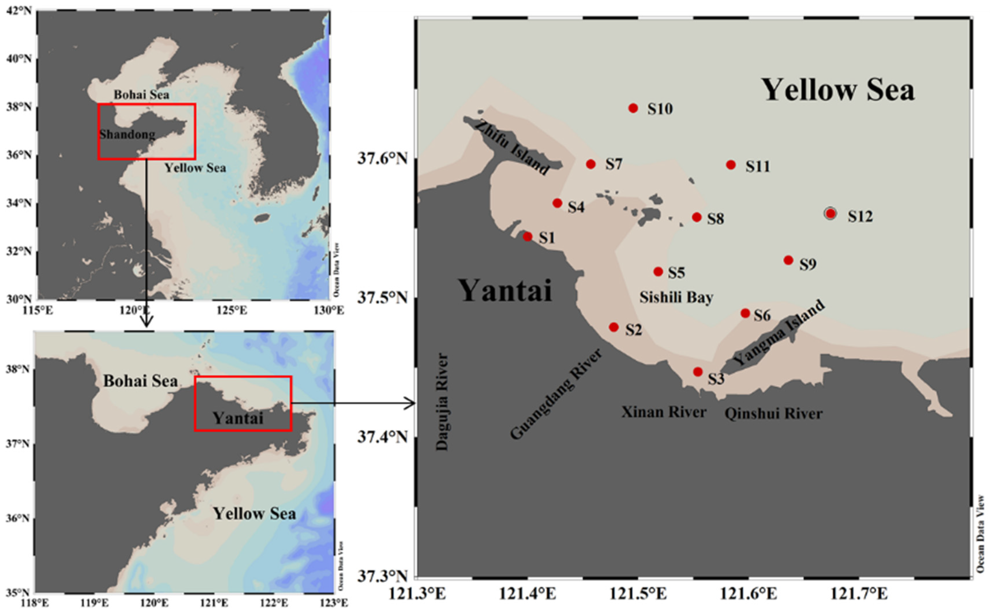
2. Study Area and Sampling

Sishili Bay (37.42–37.63° N, 120.35–120.63° E), semi-enclosed by Yantai, covers an area of 130 km2 with a 20 km long coastline. The average water depth is about 8–10 m. It is an important harbor in Northern China and provides the local seafood supply. Several rivers flow into Sishili Bay, including the Dagujia River, Guangdong River, Xin’an River, and Qinshui River. These rivers carry large amounts of nutrients and pollutants into the bay, influencing seawater quality and further affecting phytoplankton growth [30].
For this study, surface seawater samples were collected from Sishili Bay (Figure 1) over four years. Samples were collected on a wooden boat approximately 10 m long at a sea depth of 0.5 m, using a polytetrafluoroethylene sampler with a capacity of 1 L. Samples were collected in 2017 (February, March, June, July, October, November), 2018 (March, May, July, September, November), 2019 (May, June, July, August, September, November), and 2020 (June, August). The following parameters were simultaneously measured in the seawater samples at every station using a YSI Water Quality Analyzer (ProPlus): temperature (T), salinity (SAL), dissolved oxygen (DO), conductivity (Cond), and pH value. After collection, the samples were immediately filtered through a 0.45 μm-pore filter. The filtered membranes were wrapped in aluminum foil, and stored at −20 °C until measurement of chlorophyll a (Chl a). The filtrates were then frozen in 1 L clean polytetrafluoroethylene (PTFE) bottles until measurement.

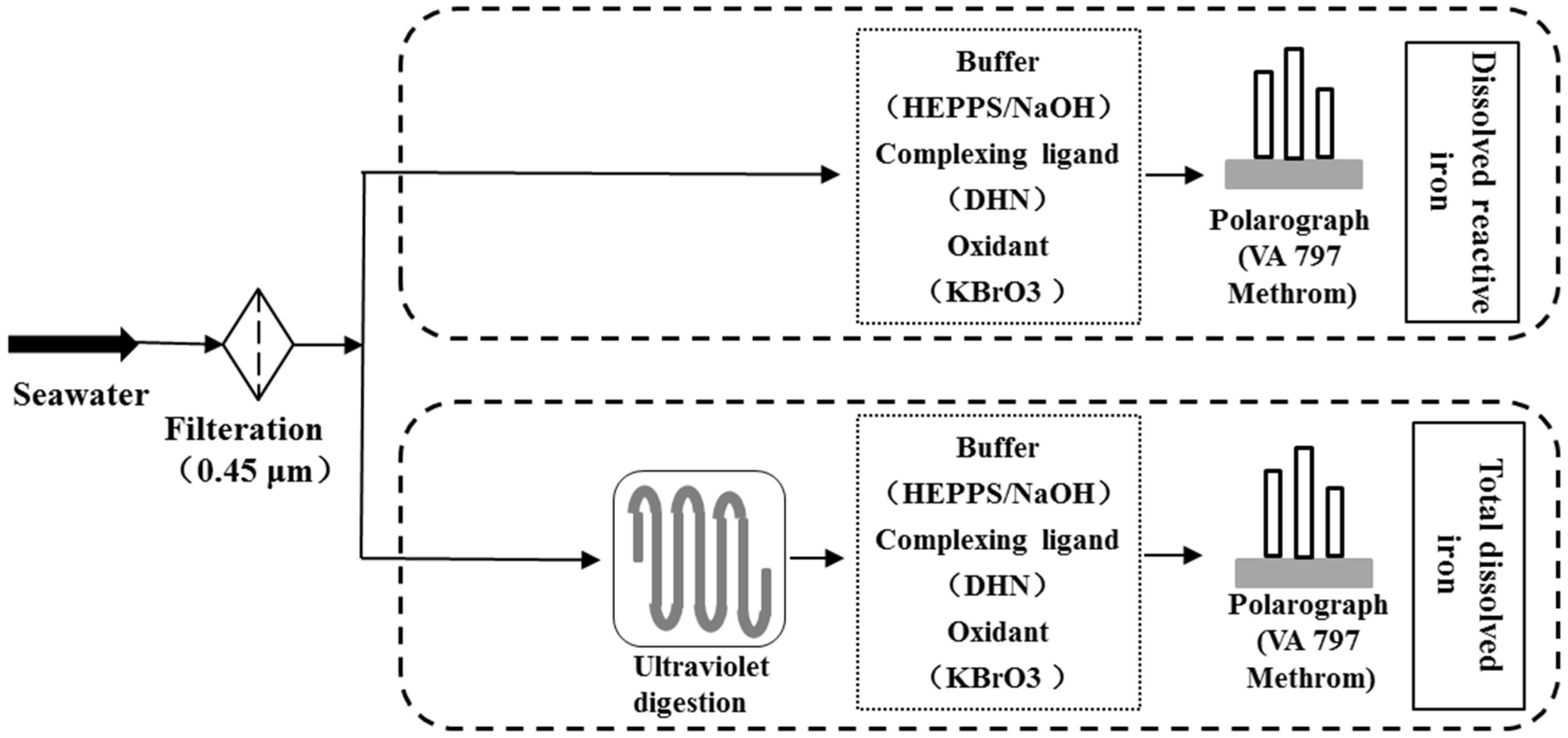
3. Materials and Methods

The electrochemical experiments were conducted using a 797 VA Computrace instrument (Metrohm, Herisau, Switzerland). Samples (10 mL) were placed in a Teflon voltammetric cell and were then stirred using a rotating Teflon rod. A hanging mercury drop electrode (HMDE) was used as a working electrode; the reference electrode was silver/silver chloride (Ag/AgCl) with 3 mol/L potassium chloride (KCl), while platinum (Pt) was used as the auxiliary electrode. The pH of the solution used in the experiment was debugged using a FE 28 pH meter (Mettler-Toledo International Trade Limited Company, Shanghai, China). A Model 705 ultraviolet digestion instrument (Metrohm, Herisau, Switzerland) was used for sample digestion. The physical and chemical parameters of seawater were measured using a YSI ProPlus Multiparameter Water Quality Measuring Instrument (Proplus, Dublin, Ireland). The concentration of Chl a was determined using a Turner Designs Trilogy fluorimeter, following the detailed steps described in a previous study by our team [29]. The concentrations of nitrates and phosphates were determined using flow injection analysis (QuAAtro, Bran+Luebbe, Hamburg, Germany).
Ultrapure water was used in the experiments, produced by PURELAB Classic UV (ELGA LabWater, High Wycombe, UK). The reagents used in the experiment were all guaranteed reagents. A stock solution of DHN (2,3-dihydroxynaphthalene) (>98% purity, Sigma-Aldrich, St. Louis, MO, USA) was prepared in methanol at a concentration of 20 mM, with 10 μL added as a complexant at a final concentration of 20 μM in 10 mL sample when testing. A 1 M HEPPS (4-(2-hydroxyethyl)-1-piperazine propionic sulfonic acid solution; Sigma-Aldrich, St. Louis, MO, USA) was prepared in 0.5 M NaOH as a buffer solution. A 0.4 M potassium bromate (KBrO3) solution was prepared as a catalytic agent. These three solutions were purified using a MnO2 solution [31,32]. A standard solution of Fe (III) was created in a 0.1 M HCl solution. The full experiment was conducted in a class-100 clean laminar flow bench to avoid contaminating the reagents. The utensils used in the experiment were soaked in 5% high-grade pure HNO3 for at least 24 h, then washed thoroughly with deionized water and dried for later use.
The iron speciation was determined using CSV [31,33]. Figure 2 shows a flow chart for determining the different species of iron in seawater. The concentration of dissolved reactive iron (DrFe) includes all dissolved inorganic iron (II and III) and part of the organically complexed iron, while that of TdFe includes all dissolved inorganic and organic iron [34]. DrFe was determined by adding 10 mL filtered seawater sample without pretreatment to a quartz voltammetric cell with 100 μL of a 1 M HEPPS/0.5 M NaOH buffer solution (keeping the pH value of the determination system at about 8.0). Following this, 10 μL of 20 mM DHN and 500 μL of 0.4 M KBrO3 were sequentially added. The electrochemical detection experiment was performed after 5 min of oxygen removal using high purity nitrogen. The concentrations of DrFe in seawater were measured using a standard addition method [25,26,31], and a graphical representation of titration was shown in Figure S3. As compared, the detection process of TdFe was similar to the process used to detect DrFe, except that filtered samples were digested for 90 min at pH 2 under a high-pressure mercury vapor lamp to destroy the complexes and compounds prior to analysis [35].
The detailed parameters of the differential pulse stripping voltammetry were as follows: the initial potential was −0.1 V; the final potential was −1.1 V; the sweep rate was 24 m V/s; the deposition potential was −0.1 V; the deposition time was 60 s and the equilibrium time was 5 s. Each sample was measured three times. The limit of detectable concentration of this method was 0.02 nM. The iron content in standard seawater samples (CASS-5 and NASS-6) was measured in comparison. The specific results of the method have been described in a previous study by our team [36].

4. Results and Discussion

4.1. Hydrographic Properties

Table 1 provides the typical average values of T, DO, Cond, SAL, pH, and Chl a for the seawater samples in Sishili Bay in 2018. The results showed that there were seasonal variations in T, DO, and Chl a. However, the Cond, SAL, and pH values exhibited little difference over five months. The average T was highest in July, with sequentially decreasing values in September, May, November, and March. The Chl a levels were highest in September, with sequentially decreasing values in July, May, November, and March. This change order was generally consistent with that of T. However, the DO levels were almost on the contrary order. These levels were highest in March, with sequentially decreasing values in May, November, July, and September. In summary, T was in the same variation trend with Chl a and was in the opposite trend with DO. These results were generally consistent with previous studies [37,38], which may be because as the T increased, phytoplankton grew more vigorously, and the solubility of DO decreased. The temporal and spatial distribution of Chl a and the correlation between DrFe and physicochemical parameters are given in the supporting manuscript [39,40,41].

4.2. Comparison of TdFe in Sishili Bay with Other Coastal Areas

Table 2 lists the average levels and the range of different species of iron over the five monitoring months in 2018. TdFe levels provided by our previous work ranged from 27.8 to 82.0 nM with decreasing values in March, November, September, July, and May [29], and DrFe content ranged from 6.8 to 13.3 nM with decreasing values in September, May, July, March, and November, the proportion of DrFe to TdFe ranging from 10.4% to 47.7%. As shown in Figure 3A,B and Figure 4, DrFe changed little, while the variation trend of TdFe was opposite to and the proportion of DrFe to TdFe. It could be concluded that DrFe content in 2018 was relatively stable compared to that of TdFe.
There is insufficient research about TdFe levels in Sishili Bay to facilitate comparisons with this study, and the same is true for DrFe; because of this, TdFe concentrations were compared with those in other coastal areas (Table 3), which was also possible to further understand the level of TdFe in coastal seawater. As DrFe was rarely studied in other areas, there was no comparison of DrFe. The TdFe results were comparable with those of East China Sea, Jiaozhou Bay, and Southern Yellow Sea (Table 3) [8,22,42], while iron contents from Sanggou Bay and two foreign coastal areas were much lower in comparison (Table 3). Table 3 shows that TdFe levels in seawater from sampling stations in the East China Sea were higher in spring than in autumn. The seasonal variation in iron levels may be influenced by two current systems (the Taiwan Warm Current (TWC) and the East China Sea Coastal Current (ECSCC)), the growth of phytoplankton in spring and summer, and monsoons [22]. The TdFe concentrations were higher in summer than in spring in Jiaozhou Bay. This may be due to rainfall and the river input in summer in this area, as well as the seasonal differences in T and nutrient concentrations [8]. The TdFe concentrations were highest in spring and lower in the other three seasons in the Southern Yellow Sea, which was found to be related to physical and biogeochemical processes like spring snowmelt, summer blooms of green tides, and the winter monsoon [42]. The TdFe concentrations were also highest in spring, followed by a decrease in summer and autumn and then a slight increase in winter in Sanggou Bay (SGB), which had something to do with higher primary production in summer, the dry deposition in winter and spring, and the faster water exchange rate between SGB and the Yellow Sea in autumn [43]. Concentrations of TdFe were much lower in wet-warm seasons (May, July, and September) than in dry-cold seasons (March and November) in Sishili Bay, as presented in Table 2. Chl a concentrations in wet-warm seasons were much higher than in dry-cold seasons, as shown in Table 1, with sequentially decreasing values in September, July, May, November, and March. Results are similar to those in Peconic Estuary and other coastal areas [44]. Dissolved organic carbon (DOC) contents were in the decreasing order of September, June, May, and November in 2019 in both the mariculture area and non-mariculture area of Yantai Sishili Bay [45]. The same variation trend of TOC and Chl a with the opposite variation trend of TdFe in Sishili Bay indicated that phytoplankton were importantly involved in the DOC production [46]. The same variation trend of TOC and DrFe showed that there was a certain correlation between TOC and DrFe, which needs to be verified by further experiment.
The water circulation in the Northern Yellow Sea (NYS) is dominated by the Yellow Sea Warm Current (YSWC), the Liaonan Coastal Current (LNCC), and the Lubei Coastal Current (LBCC) [47,48]. The YSWC and LBCC are both strongest in winter and weakest (or absent) in summer. The LBCC, flowing from west to east along the northern coastal water of the Shandong peninsula and passing the sea area near Sishili Bay, transports sediment from the Yellow River delta in winter from west to east, which will increase the iron content to some extent [49,50]. The YSWC may intrude into the NYS and even into the Bohai Sea during winter and has a suspended sediment load of 3 × 10⁶ t/a, of which one-third is transported to the NYS [51]. This may also increase iron levels. Rainfall was higher in July, September, and November than in March and May of 2018 in Yantai “Yantai statistical yearbook. Available online: http://tjj.yantai.gov.cn/art/2021/1/11/art_118_2876126.html (accessed on 1 June 2022)”, which may increase iron contents in July, September and November compared to the other two months. TdFe contents were higher in dry-cold seasons (March and November) rather than in wet-warm seasons (May, July, and September), which was also probably due to the mixing of surface and bottom water, atmospheric precipitation, and relatively small biomass in dry-cold seasons, allowing TdFe to be accumulated in seawater [52,53]. In general, Iron levels are impacted by different environmental factors; as such, seasonal variations in iron levels in different regions may differ slightly.
Table 3. Comparison of dissolved iron in Sishili Bay with other regions.
LocationSampling TimeDissolved Iron
(Unit: nM)
MethodReference
Jiaozhou Bay, Yellow SeaMay 201135.2 ± 23.4CSV[8]
July 201131.1 ± 10.3
East China SeaMarch–April 201139.4 ± 26.6CSV[22]
October–November 201120.5 ± 11.0
Southern Yellow SeaJuly 20131.7–15.8CSV[42]
November 20130.9–38.5
April 20143.0–69.8
January 20163–100.2
Sanggou Bay, Yellow SeaApril12.0 ± 6.29ICP-MS[43]
July5.00 ± 2.92
October1.83 ± 0.42
January3.36 ± 2.06
Coastal Ross SeaJanuary 20140.5–4.5ICP-MS[54]
Liverpool BayApril 20144.8 ± 0.5CSV[55]
Yantai Sishili Bay, Northern Yellow SeaMarch 201858.9 ± 11.7CSVThis study
May 201839.1 ± 6.4
July 201842.1 ± 7.6
September 201846.2 ± 10.5
November 201855.1 ± 11.5
CSV, cathodic stripping voltammetry; ICP-MS, inductively coupled plasma mass spectrometry.

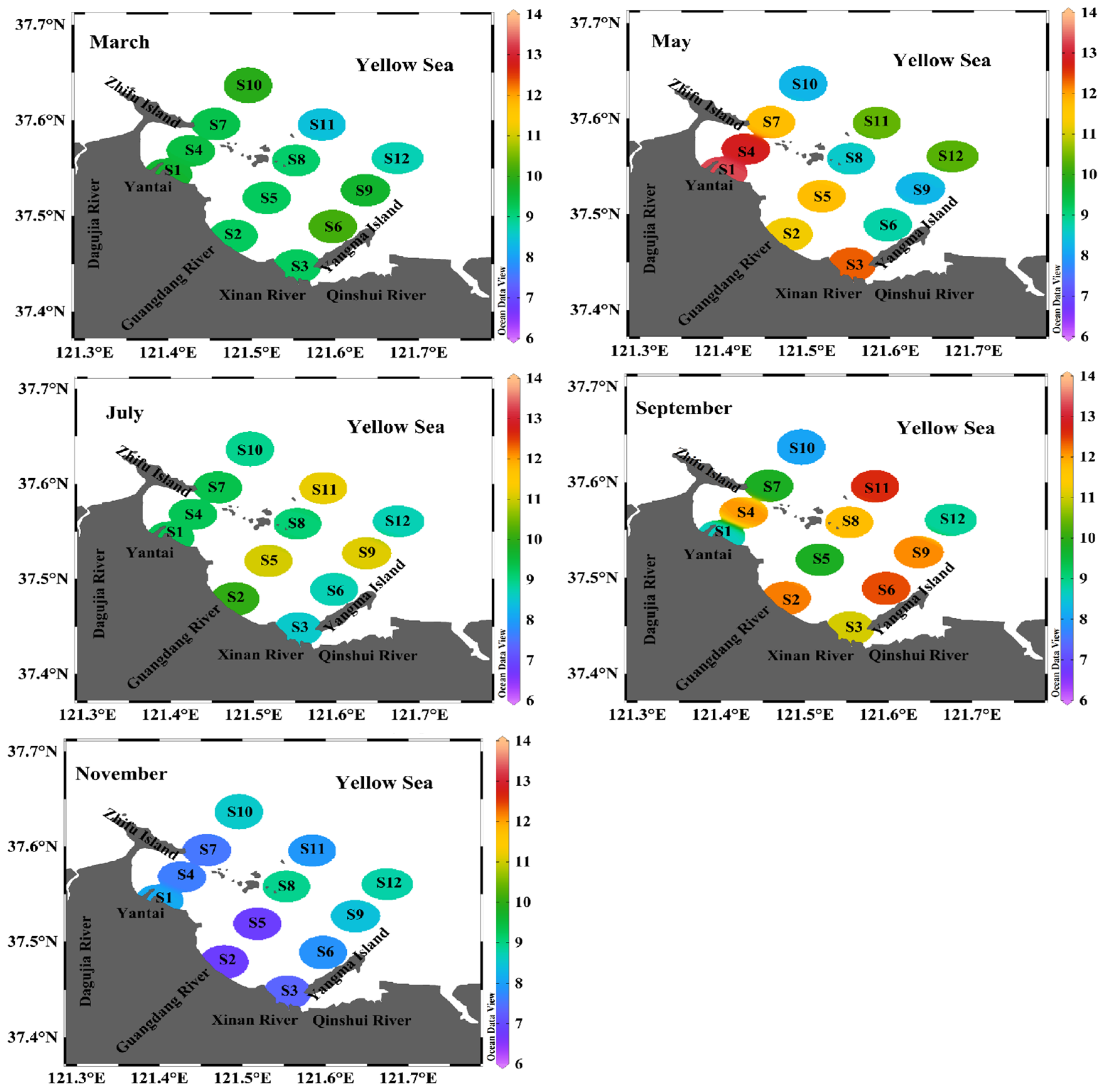
4.3. Spatial Distribution Characteristics of DrFe

Since this study mainly focused on DrFe, the spatial and temporal distribution of TdFe is not discussed in detail. The spatial distribution of DrFe is shown in Figure 5. DrFe contents varied little at different sampling sites in the same month, especially in March, July, and November, with a concentration range of 8.5–10.2 nM, 8.6–11.2 nM, and 6.8–8.8 nM, respectively. DrFe contents varied slightly more within the month in May and September than in the other three months, with a concentration range of 8.3–13.3 nM and 8.1–12.6 nM, respectively. The highest DrFe concentrations at sites S1, S3, and S4 were detected in May, at levels of 13.3 nM, 12.4 nM, and 12.8 nM, respectively. The highest DrFe concentrations at sites S2, S6, and S11 were detected in September, at levels of 12.2 nM, 12.5 nM, and 12.6 nM.
Sites S1 and S4 were close to Yantai Harbor, while S3 was in the neighboring Xin’an River Sewage Treatment Plant, which may be due to those transport activities in Yantai Harbor being more active and the quantity of wastewater effluent being large in May. Large quantities of nutrients from sewage discharge and wastewater effluent from the harbor area are known to have been added to Yantai Sishili Bay; this includes 150 tons of total phosphorus and 1910 tons of total nitrogen every year, increasing the occurrence of red tides and jellyfish blooms [56]. This increase in nutrients also increases the absorption and utilization of DrFe, meaning that the DrFe needs to be maintained at a relatively high level to ensure the growth of phytoplankton. This was somewhat similar to the research of Gobler et al., who showed that low molecular weight iron (LMW, available for immediate algal uptake, similar to DrFe here) increased when algal biomass peaked [41]. Most residential and industrial sewage from the Laishan District, including the seriously polluted water in Guangdong River, was also treated by the Xin’an River Sewage Plant in earlier years. The plant discharges approximately 5–6 tons of sewage into Sishili Bay every day [57]. These emissions, plus the influence of near-shore human activities, further intensified iron uptake and utilization by phytoplankton.
Site S2 was close to the Guangdong River and site S6 was close to Yangma Island; these two sites are known to be seriously impacted by human activities. Site S11 was near the aquaculture zone [58], and the water temperature was suitable for fish growth in autumn; in addition, the red tide phenomenon in Sishili Bay generally occurs in August and September every year [57], corresponding to a relatively higher level of Chl a in September here (Table 1). Hence, relatively high levels of organisms and nutrients in this area amplified the production of secondary metabolic products and the growth of marine bacteria and other epiphytes, which led to a greater need for DrFe. In general, it could be deduced that the DrFe in Yantai Sishili Bay was essentially maintained at a steady level to support the growth of phytoplankton and was less affected by the surrounding environment except under special circumstances.

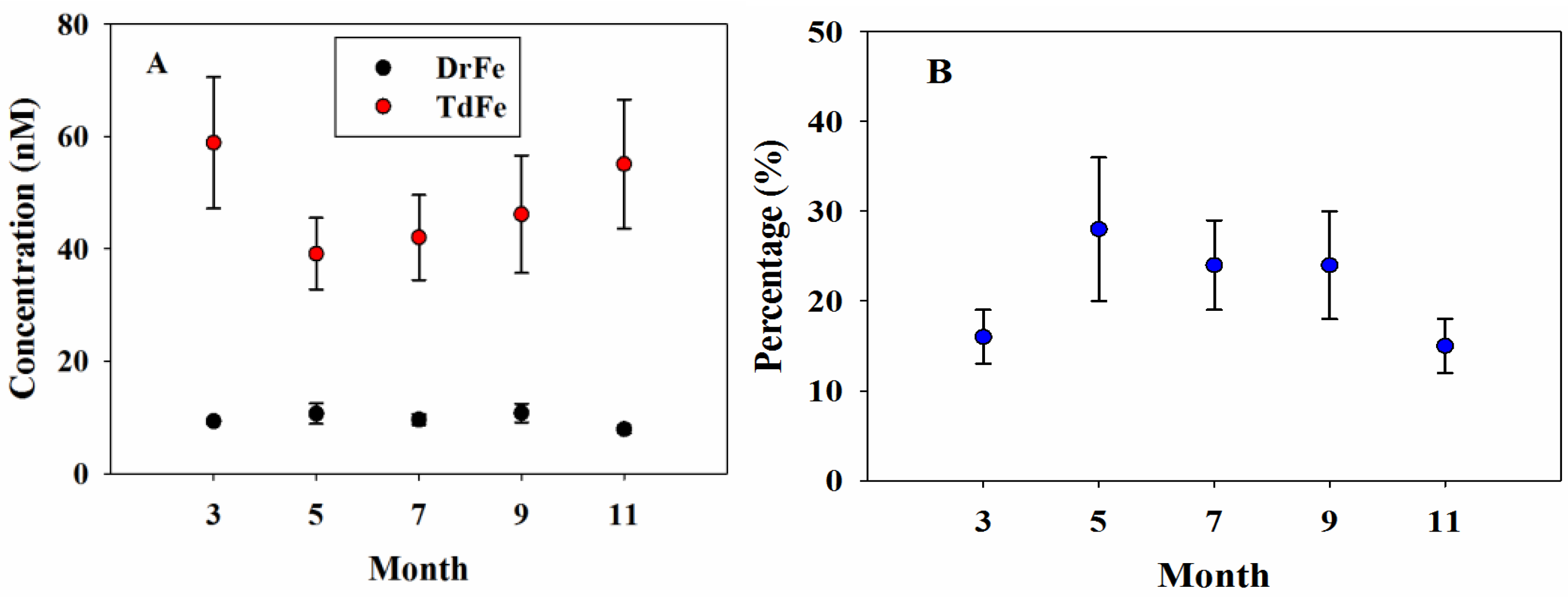
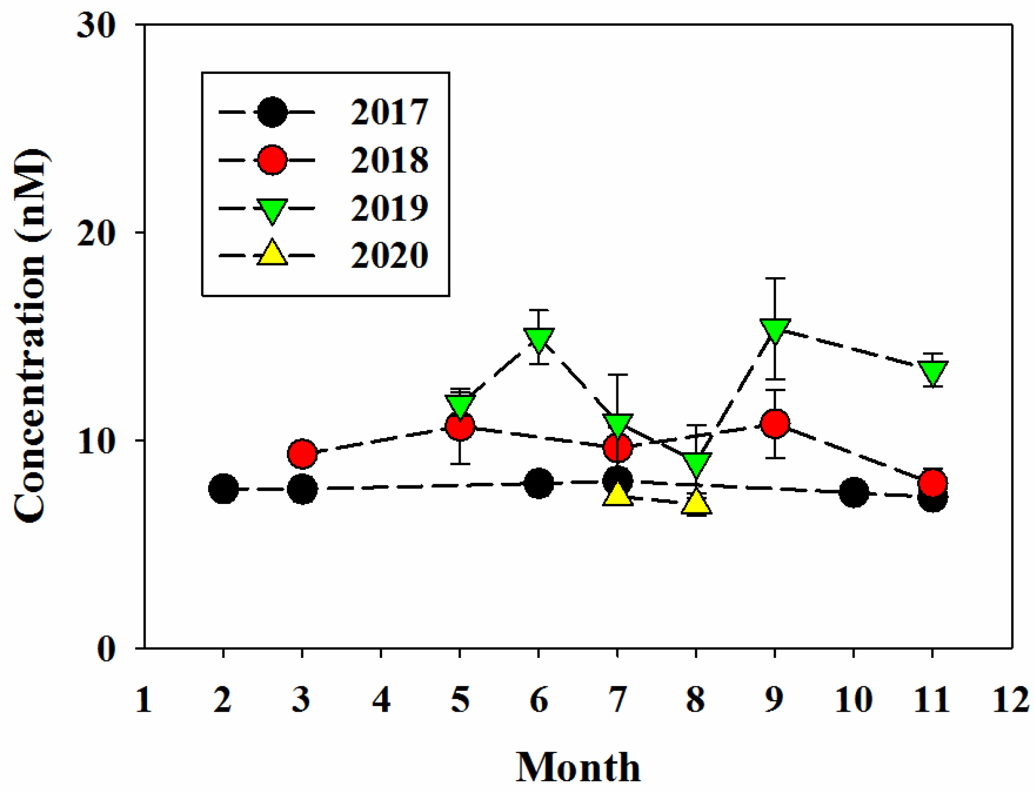
4.4. Temporal Distribution Characteristics of DrFe

Figure 6 shows that the annual change of DrFe was small in 2018, with a standard deviation of 1.0 nM and an average of 9.68 nM. The concentration of DrFe in Sishili Bay increased sequentially in November (7.9 nM), March (9.4 nM), July (9.6 nM), May (10.7 nM), and September (10.8 nM), with concentrations being relatively high in May and September. The temporal distribution of DrFe in Sishili Bay might be indirectly influenced by terrestrial input and atmospheric deposition related to seasons and climate. Yantai has a temperate monsoon climate, and data recorded by a weather observation center near Yantai City from 1971 to 2000 indicates that the average monthly precipitation peaks in August (161.6 mm) and reaches a low in February (9.7 mm). The main rainfall is concentrated between May and September. The average monthly weather temperature ranges from −1.2 to 24.8 °C, with higher temperatures recorded between May and September [59]. Seasonal rainfall may increase the land-based pollutants carried by surface runoff, raising DrFe levels. However, rainfall was the highest in July 2018 (mentioned in Section 4.2), which indicated that rainfall was not the main factor affecting the seasonal variation of DrFe. Though DrFe levels were higher in May and September compared to November, there was less variation between individual months. It can be preliminarily concluded that the content of DrFe in Sishili Bay remains stable overall within a certain concentration range.
To test this preliminary conclusion, the concentrations of DrFe in 2017, 2019, and 2020 were also measured (Figure 6). During these years, it ranged from 6.7 to 9.2 nM, 6.8–17.6 nM, and 6.3–8.0 nM, respectively; this indicates that DrFe was relatively stable except in 2019, which may be related to the test method and environment at that time. From this study, it can be reached that DrFe in coastal water can remain stable, though further study is needed to validate this observation.
Recently, two classical models were proposed to describe the kinetics of Fe uptake by phytoplankton and effectively quantify Fe availability in seawater. In the first Fe(II)s model, Fe(III) in both unchelated (Fe(III)’) and chelated (FeL) forms is reduced by surface reductases to form reduced Fe at the cell surface (Fe(II)s). Fe(II)s is a transient species that can be either transported across the cell membrane or complexed by ligands in the medium [60]. The second FeL model makes iron uptake dependent on the concentration of Fe(II) in the bulk medium and considers chelated Fe(III) (FeL) to be the only source of reduced Fe. Upon illumination, photoreduction of photolabile FeL generates unchelated reduced iron, Fe(II)’, which is rapidly oxidized to Fe(III)’ [61]. Combining these two iron uptake models and DrFe content in Sishili Bay, the relative stability of DrFe may be due to the following reason: weak chelated iron and unchelated inorganic iron could be first consumed, and complexed iron might be converted into DrFe by photoreduction and/or cell surface reduction in time to maintain the normal growth of phytoplankton [44]. Phytoplankton indeed can access Fe from strong organic ligands, such as siderophores excreted by the cells or produced by other bacterial or fungal species, through direct metal exchange accomplished by the ternary complex formed by iron chelator and acceptor [62]; but as long as DrFe concentrations are high enough, which is the case in this study as confirmed in Section 4.6 below, the consumption of Fe from strong ligands will be negligible [63]. Even so, the Fe(II)s model is the dominant but not the only iron uptake mechanism in this study, as several studies have strongly suggested that no one model can account for all iron uptake, with several different iron uptake mechanisms coexisting in a single species [62,64].

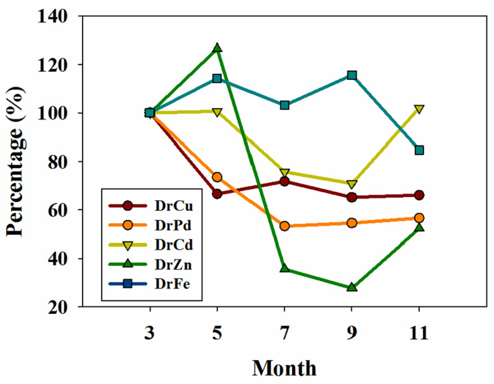
4.5. Correlation between DrFe, TdFe, and Dissolved Reactive Metals

The growth of organisms in marine environments is affected by many factors, including the concentrations and speciation of trace metals, nutrient content, and various physicochemical parameters. Cu, Pb, Cd, and Zn are essential metals for the growth of organisms in marine environments but are also the main elements causing marine metal pollution. Dissolved reactive metals (DrCu, DrPd, DrCd, DrZn) were also detected previously in our team by anodic stripping voltammetry (ASV) in filtered seawater without any reagents [29]. Because of this, it is of vital importance to explore the relationships between the different reactive metal elements. To do this, a Pearson correlation matrix was generated for DrFe, TdFe, and the other dissolved reactive metals, calculated using SPSS. As can be seen from the correlation analysis results in Table S1, there were no significant correlations among DrFe, TdFe, and other reactive metals.
There was no significant correlation between DrFe concentration and other dissolved reactive metals, as seen with the combined results of correlation analysis and variation trends (Figure 7 and Table S1). Overall, DrCu and DrPb decreased from March to May. DrCu content changed little from May to November, and DrPb content decreased from May to July before stabilizing. DrZn and DrCd followed similar trends, with relatively low concentrations in July and September. The variations in the dissolved reactive metal concentrations (DrCu, DrPb, DrCd, DrZn) were similar to that of total dissolved metals (TdCu, TdPb, TdCd, TdZn) [29]; this may be because the mean percentages of DrCu, DrPb, DrCd, and DrZn were almost greater than 60%. Because of the lack of significant correlation, the interaction between iron, these four metals, and other biogeochemical processes in Sishili Bay needs to be deeply studied with further investigation in the future.

4.6. Bioavailability of DrFe

The Fe* tracer has been used in order to indicate whether primary productivity in surface waters may be limited by iron concentrations [65], and is defined as the concentration of iron minus the expected biological Fe consumption based on the biological consumption of all ambient phosphates (PO43−) (Equation (1)) or nitrates (NO3) (Equation (2)):
F e ( P ) = [ F e ] ( ( F e P ) a l g a l   u p t a k e   r a t i o × [ P O 4 ] )
F e ( N ) = [ F e ] ( ( F e N ) a l g a l   u p t a k e   r a t i o × [ N O 3 ] )
Fe* was calculated using the global average Fe/P algal uptake ratio of 0.47 mmol/mol or with a Fe/N algal uptake ratio of 0.039 mmol/mol, derived from an assumed fixed stoichiometry based on the Redfield ratio of P:N = 1:12 [66]. Positive Fe* indicates that Fe concentrations are theoretically sufficient to completely consume PO43− or NO3 and iron is not a limiting factor for phytoplankton growth. Negative Fe* indicates that Fe concentrations are insufficient for complete consumption of PO43− or NO3, and primary productivity is potentially Fe limited.
Whether or not the DrFe levels could satisfy the growth of phytoplankton in Yantai Sishili Bay was preliminarily examined using the theoretical calculation of Fe*. As shown in Table 2, the concentration of DrFe in 2018 ranged from 6.8–13.3 nM. Due to sample handling errors in July and September, the concentrations of PO43− and NO3 were only obtained in March, May, and November. The concentration of DrFe was used to calculate the value of Fe*, the average of which can be seen in Table 4. It was calculated that the values of Fe* were much higher than zero (Table 4), which indicated that DrFe was sufficient to support the full consumption of available N and P in Sishili Bay during 2018. Since the concentration of DrFe did not differ much over the four years, with the annual mean concentration ranging from 7.1 to 12.6 nM, DrFe in Sishili Bay might have been sufficient to meet the phytoplankton demand, and it can be preliminarily concluded that iron is not a limiting factor for phytoplankton growth in this offshore area. More work must be conducted to confirm this conclusion, as well as to study the mechanism of action and bioavailability of different iron species in offshore areas at different depths.

5. Conclusions

This study investigated different iron species present in the coastal seawater of Yantai Sishili Bay over five months in 2018, including TdFe and DrFe. TdFe levels were lower during the wet-warm seasons (May, July, September) compared to the dry-cold seasons (March, November), while DrFe changed little. The main reason for the change in TdFe and steady values of DrFe might be a conversion of TdFe to DrFe due to cell surface reduction by phytoplankton and photoreduction of strong Fe-organic complexes. From the availability calculation of DrFe and nutrients, it could be preliminarily concluded that DrFe concentrations in the coastal seawater were sufficient to meet the phytoplankton demand in Yantai Sishili Bay. In the future, Fe in the seawater of Yantai Sishili Bay should continue to be assessed to analyze annual variations and provide additional scientific data to support environmental monitoring and economic development. Due to the highly heterogeneous nature of Fe, detailed characterization of various Fe species is needed to understand better the biogeochemical cycling of bioactive elements in aquatic systems.

Supplementary Materials

The following supporting information can be downloaded at: https://www.mdpi.com/article/10.3390/jmse10070890/s1, The supporting manuscript: The temporal and spatial distribution of Chl a and the correlation between DrFe and physicochemical parameters (Figure S1: Spatial distribution of chlorophyll a (Chl a) (unit: μg/L) in 2018 in Sishili Bay; Figure S2: Variation tendency of dissolved reactive iron (DrFe) and physicochemical parameters); Figure S3: Linear regression corresponding and differential pulse voltammograms for the determination of DrFe in one sample of Yantai Sishili Bay by standard addition method; Table S1: Correlation between DrFe and TdFe, DrCu, DrPb, DrCd, DrZn, and other parameters.

Author Contributions

Conceptualization, D.P. and C.W.; resources, H.H., S.Z. and Y.L. (Yuxi Lu); investigation, methodology, writing—original draft, C.W.; formal analysis, Y.L. (Yongsheng Luan); writing—review & editing, D.P. and Y.L. (Yuxi Lu). All authors have read and agreed to the published version of the manuscript.

Funding

This work was financially supported by the Original Innovation Project (ZDBS-LY-DQC009) and the Strategic Priority Research Program (XDB42000000) of the Chinese Academy of Sciences and the National Natural Science Foundation of China (42177443).

Institutional Review Board Statement

Not applicable.

Informed Consent Statement

Not applicable.

Data Availability Statement

Data is contained within the article.

Acknowledgments

We would like to thank Jianmin Zhao and Xiyan Sun from Muping Coastal Environment Research Station, Chinese Academy of Sciences, for providing the concentrations of phosphate and nitrate. We also thank anonymous reviewers for their valuable comments to the manuscript and their constructive suggestions.

Conflicts of Interest

The authors declare no conflict of interest.

References

  1. Taylor, S.R. Abundance of chemical elements in the continental crust a new table. Geochim. Cosmochim. Acta 1964, 28, 1273–1285. [Google Scholar] [CrossRef]
  2. Morel, F.M.M.; Price, N.M. The biogeochemical cycles of trace metals in the oceans. Science 2003, 300, 944–947. [Google Scholar] [CrossRef] [PubMed] [Green Version]
  3. Laglera, L.M.; Santos-Echeandia, J.; Caprara, S.; Monticelli, D. Quantification of iron in seawater at the low picomolar range based on optimization of bromate/ammonia/dihydroxynaphtalene system by catalytic adsorptive cathodic stripping voltammetry. Anal. Chem. 2013, 85, 2486–2492. [Google Scholar] [CrossRef] [Green Version]
  4. Behrenfeld, M.J.; Milligan, A.J. Photophysiological expressions of iron stress in phytoplankton. Annu. Rev. Mar. Sci. 2013, 5, 217–246. [Google Scholar] [CrossRef]
  5. Lu, M.; Rees, N.V.; Kabakaev, A.S.; Compton, R.G. Determination of Iron: Electrochemical Methods. Electroanalysis 2012, 24, 1693–1702. [Google Scholar] [CrossRef]
  6. Boyd, P.W.; Watson, A.J.; Law, C.S.; Abraham, E.R.; Zeldis, J. A mesoscale phytoplankton bloom in the polar Southern Ocean stimulated by iron fertilization. Nature 2000, 407, 695–702. [Google Scholar] [CrossRef]
  7. Martin, J.H.; Coale, K.H.; Johnson, K.S.; Fitzwater, S.E. The iron hypothesis: Ecosystem tests in equatorial Pacific waters. Nature 1994, 371, 123–129. [Google Scholar] [CrossRef]
  8. Su, H.; Yang, R.J.; Pižeta, I.; Omanović, D.; Wang, S.R.; Li, Y. Distribution and Speciation of Dissolved Iron in Jiaozhou Bay (Yellow Sea, China). Front. Mar. Sci. 2016, 3, 99. [Google Scholar] [CrossRef] [Green Version]
  9. Nagai, T.; Imai, A.; Matsushige, K.; Yokoi, K.; Fukushima, T. Dissolved iron and its speciation in a shallow eutrophic lake and its inflowing rivers. Water Res. 2007, 41, 775–784. [Google Scholar] [CrossRef]
  10. Hogle, S.L.; Dupont, C.L.; Hopkinson, B.M.; King, A.L.; Buck, K.N.; Roe, K.L.; Stuart, R.K.; Allen, A.E.; Mann, E.L.; Johnson, Z.I.; et al. Pervasive iron limitation at subsurface chlorophyll maxima of the California Current. Proc. Natl. Acad. Sci. USA 2018, 115, 13300–13305. [Google Scholar] [CrossRef] [Green Version]
  11. Van den Berg, C.M.G. Chemical Speciation of Iron in Seawater by Cathodic Stripping Voltammetry with Dihydroxynaphthalene. Anal. Chem. 2006, 78, 156–163. [Google Scholar] [CrossRef] [PubMed]
  12. Kondo, Y.; Takeda, S.; Furuya, K. Distinct trends in dissolved Fe speciation between shallow and deep waters in the Pacific Ocean. Mar. Chem. 2012, 134–135, 18–28. [Google Scholar] [CrossRef]
  13. Chen, M.; Dei, R.C.H.; Wang, W.H.; Guo, L.D. Marine diatom uptake of iron bound with natural colloids of different origins. Mar. Chem. 2003, 81, 177–189. [Google Scholar] [CrossRef]
  14. Hutchins, D.A.; Witter, A.E.; Butler, A.; Luther III, G.W. Competition among marine phytoplankton for diferent chelated iron species. Nature 1999, 400, 858–861. [Google Scholar] [CrossRef]
  15. Gledhill, M.; van den Berg, C.M.G.; Nolting, R.F.; Timmermans, K.R. Variability in the speciation of iron in the northern North Sea. Mar. Chem. 1998, 59, 283–300. [Google Scholar] [CrossRef]
  16. Monticelli, D.; Caprara, S. Voltammetric tools for trace element speciation in fresh waters: Methodologies, outcomes and future perspectives. Environ. Chem. 2015, 12, 683–705. [Google Scholar] [CrossRef] [Green Version]
  17. Achterberg, E.P.; Herzl, V.M.; Braungardt, C.B.; Millward, G.E. Metal behaviour in an estuary polluted by acid mine drainage: The role of particulate matter. Environ. Pollut. 2003, 121, 283–292. [Google Scholar] [CrossRef]
  18. Huang, S.B.; Wang, Z.J.; Ma, M. Measuring the bioavailable/toxic concentration of copper in natural water by using anodic stripping voltammetry and Vibrio qinghaiensis sp. Nov. Q67 bioassay. Chem. Spec. Bioavailab. 2003, 15, 37–45. [Google Scholar] [CrossRef]
  19. Campos, M.L.A.M.; van den Berg, C.M.G. Determination of copper complexation in sea water by cathodic stripping voltammetry and ligand competition with salicylaldoxime. Anal. Chim. Acta. 1994, 284, 481–496. [Google Scholar] [CrossRef]
  20. Croot, P.L.; Johansson, M. Determination of Iron Speciation by Cathodic Stripping Voltammetry in Seawater Using the Competing Ligand 2-(2-Thiazolylazo)-p-cresol (TAC). Electroanalysis 2000, 12, 565–576. [Google Scholar] [CrossRef]
  21. Rue, E.L.; Bruland, K.W. Complexation of iron(III) by natural organic ligands in the Central North Pacific as determined by a new competitive ligand equilibration. Mar. Chem. 1995, 50, 117–138. [Google Scholar] [CrossRef]
  22. Su, H.; Yang, R.J.; Zhang, A.B.; Li, Y. Dissolved iron distribution and organic complexation in the coastal waters of the East China Sea. Mar. Chem. 2015, 173, 208–221. [Google Scholar] [CrossRef]
  23. Yang, R.J.; Su, H.; Qu, S.L.; Wang, X.C. Capacity of humic substances to complex with iron at different salinities in the Yangtze River estuary and East China Sea. Sci. Rep. 2017, 7, 1381. [Google Scholar] [CrossRef] [PubMed]
  24. Sukekava, C.; Downes, J.; Slagter, H.A.; Gerringa, L.J.A.; Laglera, L.M. Determination of the contribution of humic substances to iron complexation in seawater by catalytic cathodic stripping voltammetry. Talanta 2018, 189, 359–364. [Google Scholar] [CrossRef] [PubMed]
  25. Aldrich, A.P.; van den Berg, C.M.G.; Thies, H.; Nickus, U. The redox speciation of iron in two lakes. Mar. Freshw. Res. 2001, 52, 885–890. [Google Scholar] [CrossRef]
  26. Boye, M.; Aldrich, A.; van den Berg, C.M.G.; de Jong, J.T.M.; Nirmaier, H.; Veldhuis, M.; Timmermans, K.R.; de Baar, H.J.W. The chemical speciation of iron in the north-east Atlantic Ocean. Deep Sea Res. Part I Oceanogr. Res. Pap. 2006, 53, 667–683. [Google Scholar] [CrossRef] [Green Version]
  27. Zhang, B.; Wu, D.; Yang, X.; Teng, J.; Liu, Y.L.; Zhang, C.; Zhao, J.M.; Yin, X.N.; You, L.P.; Liu, Y.F.; et al. Microplastic pollution in the surface sediments collected from Sishili Bay, North Yellow Sea, China. Mar. Pollut. Bull. 2019, 141, 9–15. [Google Scholar] [CrossRef] [PubMed]
  28. Han, H.T.; Pan, D.W.; Zhang, S.H.; Wang, C.C.; Hu, X.P.; Wang, Y.C.; Pan, F. Simultaneous Speciation Analysis of Trace Heavy Metals (Cu, Pb, Cd and Zn) in Seawater from Sishili Bay, North Yellow Sea, China. Bull. Environ. Contam. Toxicol. 2018, 101, 486–493. [Google Scholar] [CrossRef]
  29. Pan, D.W.; Ding, X.Y.; Han, H.T.; Zhang, S.H.; Wang, C.C. Species, Spatial-Temporal Distribution, and Contamination Assessment of Trace Metals in Typical Mariculture Area of North China. Front. Mar. Sci. 2020, 7, 552893. [Google Scholar] [CrossRef]
  30. Wang, Y.J.; Liu, D.Y.; Dong, Z.J.; Di, B.P.; Shen, X.H. Temporal and spatial distributions of nutrients under the influence of human activities in Sishili Bay, northern Yellow Sea of China. Mar. Pollut. Bull. 2012, 64, 2708–2719. [Google Scholar] [CrossRef]
  31. Obata, H.; van den Berg, C.M.G. Determination of Picomolar Levels of Iron in Seawater Using Catalytic Cathodic Stripping Voltammetry. Anal. Chem. 2001, 73, 2522–2528. [Google Scholar] [CrossRef] [PubMed]
  32. Yang, R.J.; Wang, S.R.; Li, J.X.; Wang, X.L. The determination of iron in sea water by cathodic stripping voltammetry. Period. Ocean Univ. China 2012, 42, 143–149. (In Chinese) [Google Scholar]
  33. Abualhaija, M.M.; van den Berg, C.M.G. Chemical speciation of iron in seawater using catalytic cathodic stripping voltammetry with ligand competition against salicylaldoxime. Mar. Chem. 2014, 164, 60–74. [Google Scholar] [CrossRef]
  34. Aldrich, A.P.; van den Berg, C.M.G. Determination of Iron and Its Redox Speciation in Seawater Using Catalytic Cathodic Stripping Voltammetry. Electroanalysis 1998, 10, 369–373. [Google Scholar] [CrossRef]
  35. Achterberg, E.P.; van den Berg, C.M.G. In-line ultraviolet-digestion of natural water samples for trace metal determination using an automated voltammetric system. Anal. Chim. Acta 1994, 291, 213–232. [Google Scholar] [CrossRef]
  36. Lin, M.Y.; Pan, D.W.; Hu, X.P.; Zhu, Y.; Han, H.T.; Li, F. Speciation analysis of iron in Yantai coastal waters. Environ. Chem. 2016, 35, 297–304. (In Chinese) [Google Scholar]
  37. Kang, J.; Chen, X.Q.; Zhang, M. The distribution of chlorophyll a and its influencing factors in different regions of the Bering Sea. Acta Oceanol. Sin. 2014, 33, 112–119. [Google Scholar] [CrossRef]
  38. Carbone, M.E.; Spetter, C.V.; Marcovecchio, J.E. Seasonal and spatial variability of macronutrients and Chlorophyll a based on GIS in the South American estuary (Bahía Blanca, Argentina). Environ. Earth Sci. 2016, 75, 736. [Google Scholar] [CrossRef]
  39. Shen, G.; Shi, B. Marine Ecology; Science Press: Beijing, China, 2002; pp. 100–230. (In Chinese) [Google Scholar]
  40. Herzog, S.D.; Persson, P.; Kritzberg, E.S. Salinity Effects on Iron Speciation in Boreal River Waters. Environ. Sci. Technol. 2017, 51, 9747–9755. [Google Scholar] [CrossRef]
  41. Lippiatt, S.M.; Lohan, M.C.; Bruland, K.W. The distribution of reactive iron in northern Gulf of Alaska coastal waters. Mar. Chem. 2010, 121, 187–199. [Google Scholar] [CrossRef]
  42. Zhu, M.H.; Yang, R.J.; Li, Y.; Su, H.; Shan, Q.Q.; Ning, Y.T.; Fu, S.L.; Wang, S.R. Seasonal and spatial variabilities of dissolved iron in southern Yellow Sea. Chemosphere 2020, 256, 126856. [Google Scholar] [CrossRef] [PubMed]
  43. Zhu, X.C.; Zhang, R.F.; Liu, S.M.; Wu, Y.; Jiang, Z.J.; Zhang, J. Seasonal distribution of dissolved iron in the surface water of Sanggou Bay, a typical aquaculture area in China. Mar. Chem. 2017, 189, 1–9. [Google Scholar] [CrossRef]
  44. Gobler, C.J.; Donat, J.R.; Consolvo, J.A., III; Sanudo-Wilhelmy, S.A. Physicochemical speciation of iron during coastal algal blooms. Mar. Chem. 2002, 22, 71–89. [Google Scholar] [CrossRef]
  45. Yang, B.; Gao, X.L.; Zhao, J.M.; Xie, L.; Liu, Y.L.; Lv, X.Q.; Xing, Q.G. The impacts of intensive scallop farming on dissolved organic matter in the coastal waters adjacent to the Yangma Island, North Yellow Sea. Sci. Total Environ. 2022, 807, 150989. [Google Scholar] [CrossRef]
  46. Li, H.M.; Zhang, Y.Y.; Liang, Y.T.; Chen, J.; Zhu, Y.C.; Zhao, Y.T.; Jiao, N.Z. Impacts of maricultural activities on characteristics of dissolved organic carbon and nutrients in a typical raft-culture area of the Yellow Sea, North China. Mar. Pollut. Bull. 2018, 137, 456–464. [Google Scholar] [CrossRef]
  47. Yang, B.; Gao, X.L.; Zhao, J.M.; Liu, Y.L.; Gao, T.C.; Lui, H.-K.; Huang, T.-H.; Chen, C.-T.A.; Xing, Q.G. The influence of summer hypoxia on sedimentary phosphorus biogeochemistry in a coastal scallop farming area, North Yellow Sea. Sci. Total Environ. 2021, 759, 143486. [Google Scholar] [CrossRef]
  48. Yang, B.; Gao, X.L.; Zhao, J.M.; Liu, Y.L. Summer deoxygenation in a bay scallop (Argopecten irradians) farming area: The decisive role of water temperature, stratification and beyond. Mar. Pollut. Bull. 2021, 173, 113092. [Google Scholar] [CrossRef]
  49. Li, Z.; Bao, X.W.; Wang, Y.Z.; Li, N.; Qiao, L.L. Seasonal distribution and relationship of water mass and suspended load in North Yellow Sea. Chin. J. Oceanol. Limnol. 2009, 27, 907–908. [Google Scholar] [CrossRef]
  50. Zhang, Y.; Gao, X.L.; Guo, W.D.; Zhao, J.M.; Li, Y.F. Origin and Dynamics of Dissolved Organic Matter in a Mariculture Area Suffering from Summertime Hypoxia and Acidification. Front. Mar. Sci. 2018, 5, 325. [Google Scholar] [CrossRef]
  51. Chen, X.H.; Li, T.G.; Zhang, X.H.; Li, R.H. A Holocene Yalu River-derived fine-grained deposit in the southeast coastal area of the Liaodong Peninsula. Chin. J. Oceanol. Limnol. 2013, 31, 636–647. [Google Scholar] [CrossRef]
  52. Ma, K.Y.; Yang, R.J.; Qu, S.L.; Zhang, Y.Y.; Liu, Y.; Xie, H.; Zhu, M.H.; Bi, M.Q. Evidence for coupled iron and nitrate reduction in the surface waters of Jiaozhou Bay. J. Environ. Sci. 2021, 108, 70–83. [Google Scholar] [CrossRef] [PubMed]
  53. Xie, L.; Gao, X.L.; Liu, Y.L.; Yang, B.; Lv, X.Q.; Zhao, J.M.; Xing, Q.G. Atmospheric dry deposition of water-soluble organic matter: An underestimated carbon source to the coastal waters in North China. Sci. Total Environ. 2022, 818, 151772. [Google Scholar] [CrossRef] [PubMed]
  54. Rivaro, P.; Ardini, F.; Grotti, M.; Aulicino, G.; Cotroneo, Y.; Fusco, G.; Mangoni, O.; Bolinesi, F.; Saggiomo, M.; Celussi, M. Mesoscale variability related to iron speciation in a coastal Ross Sea area (Antarctica) during summer 2014. Chem. Ecol. 2018, 35, 1–19. [Google Scholar] [CrossRef]
  55. Mahmood, A.; Abualhaija, M.M.; van den Berg, C.M.G.; Sander, S.G. Organic speciation of dissolved iron in estuarine and coastal waters at multiple analytical windows. Mar. Chem. 2015, 177, 706–719. [Google Scholar] [CrossRef]
  56. Dong, Z.J.; Liu, D.Y.; Keesing, J.K. Jellyfish blooms in China: Dominant species, causes and consequences. Mar. Pollut. Bull. 2010, 60, 954–963. [Google Scholar] [CrossRef]
  57. Hao, Y.J.; Tang, D.L.; Yu, L.; Xing, Q.G. Nutrient and chlorophyll a anomaly in red-tide periods of 2003–2008 in Sishili Bay, China. Chin. J. Oceanol. Limnol. 2011, 29, 664–673. [Google Scholar] [CrossRef]
  58. Li, B.Q.; Keesing, J.K.; Liu, D.Y.; Han, Q.X.; Wang, Y.J.; Dong, Z.J.; Chen, Q. Anthropogenic impacts on hyperbenthos in the coastal waters of Sishili Bay, Yellow Sea. Chin. J. Oceanol. Limnol. 2013, 31, 1257–1267. [Google Scholar] [CrossRef]
  59. Dong, Z.J.; Liu, D.Y.; Wang, Y.J.; Di, B.P. Temporal and spatial variations of coastal water quality in Sishili Bay, northern Yellow Sea of China. Aquat. Ecosyst. Health 2019, 22, 30–39. [Google Scholar] [CrossRef]
  60. Shaked, Y.; Kustka, A.B.; Morel, F.M.M. A general kinetic model for iron acquisition by eukaryotic phytoplankton. Limnol. Oceanogr. 2005, 50, 872–882. [Google Scholar] [CrossRef] [Green Version]
  61. Morel, F.M.M.; Kustka, A.B.; Shaked, Y. The role of unchelated Fe in the iron nutrition of phytoplankton. Limnol. Oceanogr. 2008, 53, 400–404. [Google Scholar] [CrossRef] [Green Version]
  62. Sutak, R.; Camadro, J.M.; Lesuisse, E. Iron Uptake Mechanisms in Marine Phytoplankton. Front. Microbiol. 2020, 11, 566691. [Google Scholar] [CrossRef] [PubMed]
  63. Cabanes, D.J.E.; Blanco-Ameijeiras, S.; Bergin, K.; Trimborn, S.; Völkner, C.; Lelchat, F.; Hassler, C.S. Using Fe chemistry to predict Fe uptake rates for natural plankton assemblages from the Southern Ocean. Mar. Chem. 2020, 225, 10853. [Google Scholar] [CrossRef]
  64. Morrissey, J.; Sutak, R.; Paz-Yepes, J.; Tanaka, A.; Moustafa, A.; Veluchamy, A.; Thomas, Y.; Botebol, H.; Bouget, F.Y.; McQuaid, J.B.; et al. A Novel Protein, Ubiquitous in Marine Phytoplankton, Concentrates Iron at the Cell Surface and Facilitates Uptake. Curr. Biol. 2015, 25, 364–371. [Google Scholar] [CrossRef] [Green Version]
  65. Holmes, T.M.; Wuttig, K.; Chase, Z.; van der Merwe, P.; Townsend, A.T.; Schallenberg, C.; Tonnard, M.; Bowie, A.R. Iron availability influences nutrient drawdown in the Heard and McDonald Islands region, Southern Ocean. Mar. Chem. 2019, 211, 1–14. [Google Scholar] [CrossRef]
  66. Parekh, P.; Follows, M.J.; Boyle, E.A. Decoupling of iron and phosphate in the global ocean. Glob. Biogeochem. Cycles 2005, 19, 1–16. [Google Scholar] [CrossRef]
Figure 1. Locations of seawater sampling stations in Sishili Bay.
Jmse 10 00890 g001
Figure 2. Schematic diagram of the iron speciation analysis in coastal seawater.
Jmse 10 00890 g002
Figure 3. (A) Temporal distribution of dissolved reactive iron (DrFe) and total dissolved iron (TdFe) in Sishili Bay in 2018 (nM, monthly average values); (B) Variation trend of the proportion of DrFe to TdFe.
Jmse 10 00890 g003
Figure 4. The proportion of dissolved reactive iron (DrFe) to total dissolved iron (TdFe) in Sishili Bay in different months of 2018.
Jmse 10 00890 g004
Figure 5. Spatial distribution of dissolved reactive iron (DrFe) (unit: nM) in Sishili Bay in different months of 2018.
Jmse 10 00890 g005
Figure 6. The change in dissolved reactive iron (DrFe) concentrations (unit: nM) over four years (2017–2020) in Sishili Bay.
Jmse 10 00890 g006
Figure 7. The concentration trends of dissolved reactive Cu, Pb, Cd, Zn, and Fe (DrCu, DrPb, DrCd, DrZn, DrFe) in Sishili Bay in 2018. Percentage values indicate the change in the metal concentrations in other months compared with the first months (where the first month’s concentration is set equal to 100%) [29].
Jmse 10 00890 g007
Table 1. The average physicochemical parameters in Sishili Bay in 2018.
TimeT
°C
DO
mg/L
Cond
mS/cm
SAL
PSU
pHChl a
μg/L
March3.9 ± 0.313.4 ± 1.750.1 ± 0.631.8 ± 0.48.1 ± 0.00.1 ± 0.2
May15.6 ± 0.68.5 ± 0.848.2 ± 0.231.5 ± 0.28.1 ± 0.11.9 ± 0.8
July23.8 ± 0.86.4 ± 0.847.8 ± 1.031.1 ± 0.88.1 ± 0.13.1 ± 5.9
September23.1 ± 0.26.3 ± 0.848.3 ± 0.231.5 ± 0.18.1 ± 0.14.9 ± 5.0
November13.8 ± 0.27.9 ± 0.447.7 ± 0.431.1 ± 0.28.1 ± 0.10.3 ± 0.2
T, temperature; DO, dissolved oxygen; Cond, conductivity; SAL, salinity; Chl a, chlorophyll a.
Table 2. The average and range of different iron speciation concentrations in Sishili Bay in 2018 (unit: nM).
MarchMayJuly
AverageRangeAverageRangeAverageRange
TdFe58.9 ± 11.742.4–82.039.1 ± 6.427.9–53.342.0 ± 7.627.8–52.9
DrFe9.4 ± 0.58.5–10.210.7 ± 1.88.3–13.39.6 ± 1.08.6–11.2
SeptemberNovember
AverageRangeAverageRange
TdFe46.2 ± 10.534.0–64.955.1 ± 11.541.3–76.7
DrFe10.8 ± 1.78.1–12.67.9 ± 0.76.8–9.0
TdFe, total dissolved iron; DrFe, dissolved reactive iron.
Table 4. The average [PO4] and [NO3] levels (unit: μg/L) as well as Fe*(P) and Fe*(N) (unit: nM) in Sishili Bay in 2018.
MarchMayNovember
[PO4]4.0 ± 2.05.0 ± 1.07.0 ± 4.0
[NO3]70.0 ± 20.020.0 ± 20.030.0 ± 10.0
Fe*(P)9.3 ± 0.510.6 ± 1.87.8 ± 0.7
Fe*(N)9.2 ± 0.510.6 ± 1.87.9 ± 0.7
Publisher’s Note: MDPI stays neutral with regard to jurisdictional claims in published maps and institutional affiliations.

