Ship Dynamic Positioning Control Based on Active Disturbance Rejection Control

Abstract

Nowadays, Dynamic Positioning (DP) is applied to various tasks such as subsea pipeline laying and the requirements for the positioning performance in marine operations are higher and higher. The main objective of this paper is to design a DP controller based on the Active Disturbance Rejection Control (ADRC) to solve the problems of long response time, large overshoot and low positioning accuracy in ship positioning. Firstly, the mathematical models of the ship and environmental disturbances are established. Secondly, the basic principle of ADRC is described. Meanwhile, stability analysis of the control system is introduced. Thirdly, ADRC is improved by the fal function filter and phase prediction method which solve the problem of dither and phase delay in tracking differentiators. Finally, simulations are carried out to verify the performance of the designed ADRC and the improved ADRC. Several simulation results show that the designed ADRC can realize the fixed-point control of the ship, which effectively solves the problems of long response time, overshoot and positioning accuracy, and compared with the traditional ADRC, the improved ADRC can reduce the error of straight track control, which indicates that ADRC can meet the requirements for the positioning performance and has a strong application value.

1. Introduction

With the development of modernization and the continuous improvement of living standards, people’s demand for coal and oil is increasing. Due to resource shortages caused by the over-exploitation of terrestrial resources, people began to turn their attention to the ocean whose rich resources are of great significance for people to improve economic development and social progress. Dynamic Positioning (DP) is one of the indispensable functions of modern ships, which refers to a technology in which the ship uses its propulsion device to generate thrust to resist external interference and keep the ship in a certain position or sail along a fixed trajectory [1]. It can be applied to lots of maritime activities, such as convoy, subsea pipeline laying, exploitation of marine resources and hydrological investigation. Research on DP can make ships’ control position, heading and trajectory more accurate so that ships can realize safe and flexible operation in crowded offshore production fields without risk of damage to seabed infrastructure and risers [2]. A cable-laying vessel with DP system is shown in Figure 1 [3].

Since the 1960s, many scholars all over the world have already conducted studies on the DP. The challenges facing DP control methods are nonlinearity of the model, uncertain disturbances and complexity of the algorithm [4,5,6,7,8]. Therefore, traditional control methods may be not applicable, leading to many advanced methods being proposed to solve the above problems, such as fuzzy control, intelligent algorithm, robust control, Model Predictive Control (MPC), improved Proportional-Integral-Derivative (PID), Sliding Mode Control (SMC) and adaptive control.

• Fuzzy Control

Fuzzy control can be used in combination with other algorithms, which plays a great role in parameter problems. In [9], Xu et al. proposed a fuzzy-PID controller to solve the problems of difficult parameter adjustment and nonlinear ship dynamics. The designed controller considered the positioning error and the low frequency velocity as inputs and the Proportional-Derivative (PD) parameters as outputs of the fuzzy inference. The integral control parameters remained unchanged. The simulation results showed that the proposed fuzzy PID controller could automatically tune the control coefficients according to the positioning accuracy to reduce the percent maximum overshoot, rise time and settling time. In [10], Zhang et al. proposed an adaptive control based on neural-fuzzy networks to overcome negative effects caused by unavailable velocities and unidentified control parameters. The simulations showed that the designed controllers were capable of making the ship converge to the desired point.

2.

Intelligent Algorithm

Intelligent algorithms include many novel algorithms, such as deep reinforcement learning or Particle Swarm Optimization (PSO). In [11], Øvereng et al. introduced a DP control method based on deep reinforcement learning to solve modeling inaccuracies and computational complexity, which were numerically trained through neural networks and used an optimized learning algorithm called Proximal Policy Optimization (PPO) algorithm. The simulation results showed that the proposed method could eliminate body frame errors compared with traditional methods. In [12], Ryalat et al. proposed an Interconnection and Damping Assignment-Passivity-Based Control (IAD-PBC) controller and used PSO to obtain the gains of the IDA-PBC controller which provides an effective way to tune these gains, thus improving the control performance of DP system. The simulation showed that the states with PSO converged to the desired position and heading angle and had less overshooting.

3.

Robust Control

Robust control means that the system can maintain certain performance under parameter perturbation. In [13], Zhang et al. studied a robust anti-disturbance strategy to deal with unknown time-varying disturbances of DP system and established a disturbance observer to estimate the disturbances online. The simulation results showed that the strategy could realize the fixed point and yaw control. To solve the problems of unmeasurable speed and disturbances estimation, a Finite-Time State Observer (FTSO) and Finite-Time Feedback Control (FTFC) system based on finite-time control law were proposed in [14] by Xia et al. The simulation results demonstrated that the proposed FTSO and FTFC could provide a faster convergence speed, better disturbance and parameter perturbation rejection and higher accuracy.

4.

MPC

MPC is a special control related to the model. In [15], Li et al. applied the MPC algorithm with a state estimator to ship DP system, aiming at solving the problem of unmeasurable states and measurement noises to improve the control accuracy. The simulation results showed that the MPC controller with the state estimator had the characteristics of fast, stable and accurate responses. In [16], Zheng et al. introduced two different MPC approaches to address the nonlinear horizontal trajectory tracking problem of surface vehicles. The simulation results showed that Nonlinear MPC (NMPC) was better than Linearized MPC (LMPC) in tracking error through a comparison of tracking error of NMPC and LMPC, while NMPC took a much longer time to run the simulation.

5.

Improved PID

Due to the limitations of classical PID control, many scholars began to improve PID. A Multi-Variable (MV) PID controller was proposed by Tiwari and Krishnankutty in [17] to overcome the coupled nature of the ship system. The results showed that the force requirement of MV PID controller was minimal only with a bit of sluggishness and a slight overshoot compared with parallel PID and Linear Quadratic Regulator (LQR) controllers. Reference [9] also introduced a PID controller with fuzzy control, which reduced the percentage maximum overshoot, rise time and settling time.

6.

SMC

SMC is also called variable structure control, which is essentially a special nonlinear control. In [18,19], Ashrafiuon proposed a sliding mode control method using the first-order sliding mode surface and the second-order sliding mode surface to overcome the uncertainty of the system and enhance robustness to interference. The simulation results showed that the proposed methods could successfully make the small boat follow straight-line and circular trajectories. Tannuri et al. proposed a sliding mode control to solve the problem that the positioning performance varied with environmental or loading conditions due to the nonlinearity of the ship in [20]. This paper made use of systematic experimental tests with a scale model to verify its robustness to variations in its displacement and environmental conditions. In [21], Alattas et al. proposed an adaptive non-singular Fast Terminal Sliding Mode Control (FTSMC) with integral surface for the finite time tracking control of nonlinear systems with external disturbances. The method derived an adaptive parameter-tuning law to tackle the unknown bounded disturbances and alleviate the undesired chattering problem. In [22,23], Vu et al. adopted SMC to design controllers and proved the stability of the system based on Lyapunov criteria. The former reference proposed a robust Station-Keeping (SK) control algorithm based on SMC to tackle model uncertainties and ocean current disturbance. Besides, an optimal allocation control was also designed to keep the linear position and Euler angles. The latter reference proposed a motion control based on Dynamic Sliding Mode Control (DSMC) to improve the system robustness with the model uncertainties. Compared with the Least Square (LS) and Quadratic Programming (QP), the QP method could distribute a proper thrust and provide higher stability with smaller steady-state error and stronger robustness. In [24], Piao et al. designed a sliding mode controller based on approach law and adaptive backstepping control and added a tracking differentiator to eliminate the large chattering. Compared with traditional sliding mode control, the designed controller had a better performance on dynamic positioning under certain disturbances.

7.

Adaptive Control

Hu et al. introduced an adaptive control approach based on Dynamic Surface Control (DSC) and Minimal Learning Parameter (MLP) techniques in [25]. The proposed complete system was developed to overcome the negative effect of input saturation constraints and the singularity problem of the controller. The simulation results showed that the tracking error could converge to a small interval. In [26], Zhao et al. designed an adaptive nonlinear course controller based on the backstepping control method and dynamic surface control to solve the problems of parameter uncertainties and completely unknown control gain, but also to overcome the “explosion of terms” of the traditional backstepping control method. The simulation results showed that the method could make the error converge approximately to 0, which was proved effective. In [27], Li et al. proposed a Robust Adaptive Neural Network Control (RANNC) scheme for DP of marine vessels to overcome model uncertainties, external disturbances and input saturation. This scheme combined adaptive control and neural network, which tackled the changes of inertial matrix and damping matrix.

In the above studies, although the requirement of DP ships can be met, there are common problems of long response time, large overshoot or low positioning accuracy which may cause position deviation in laying subsea cables or oil extraction, especially when the environmental interference is large; it may cause the motion of ships to be out of control. At the same time, the ship modeling is complex and needs nonlinear approaches. Therefore, it is difficult to define their accurate kinematic and kinetic models. The Active Disturbance Rejection Control (ADRC) can overcome the dependence on the precise model and has the advantage of fast speed, and its estimation and compensation of the total disturbance can avoid the side effect of error integral feedback, which makes the signal achieve complete tracking to reduce the error and increase positioning accuracy without large overshooting. Therefore, this paper uses ADRC to realize the fixed-point control and the straight track control of the ship. For the setting of the trajectory, this paper uses a parametric equation to simplify complex problems. The objective of the fixed-point control is to keep the ships constantly near of the set position and stay berthed after reaching the set position. In the fixed-point control, through comparison between ADRC and backstepping method, it can be seen that ADRC does have a fast response speed. The objective of the straight track control is to make the ship sail along the set trajectory and minimize the error, while keeping the ship speed at the set speed. Due to the possible problems of dither and phase delay of classical ADRC, this paper is to use fal function filter and phase prediction to improve these limitations. The fal function has fast convergence and can filter out dithering well. This paper applies the fal function filter to the tracking differentiator to solve the dither problem. The phase prediction based on mathematical differential allows good phase compensation and is easy to realize. This paper combines the two methods with ADRC into dynamic positioning to improve the control performance. The simulation results demonstrate the effectiveness and practicality of the proposed controllers and their robustness to external disturbances.

The paper is constructed as follows. Firstly, Section 2 introduces the ship model including coordinate systems and mathematical models of the ship. Next, Section 3 describes the models of environmental disturbances including wind and waves. Then, Section 4 introduces the DP controller based on the basic principle of ADRC and describes the stability analysis of the control system. After that, Section 5 analyzes the problems of the controller and improves the controller by fal function filter and phase prediction. Subsequently, Section 6 presents the simulations that the designed controller is used to realize the fixed-point control and yaw control compared with backstepping method, and the effectiveness of the Improved Active Disturbance Rejection Control (IADRC) is verified under the condition of straight track control. Finally, Section 7 provides conclusions of this paper and introduces suggestions for future research.

2. Ship Model

2.1. Assumptions

To simplify the problem, this work is based on the following assumptions:

(1)

The motion of the ship in roll, pitch and heave is neglected.

(2)

The motion of the ship is regarded as a plane motion.

(3)

The water area of the ship is wide enough, and the hull draft is unchanged during the movement.

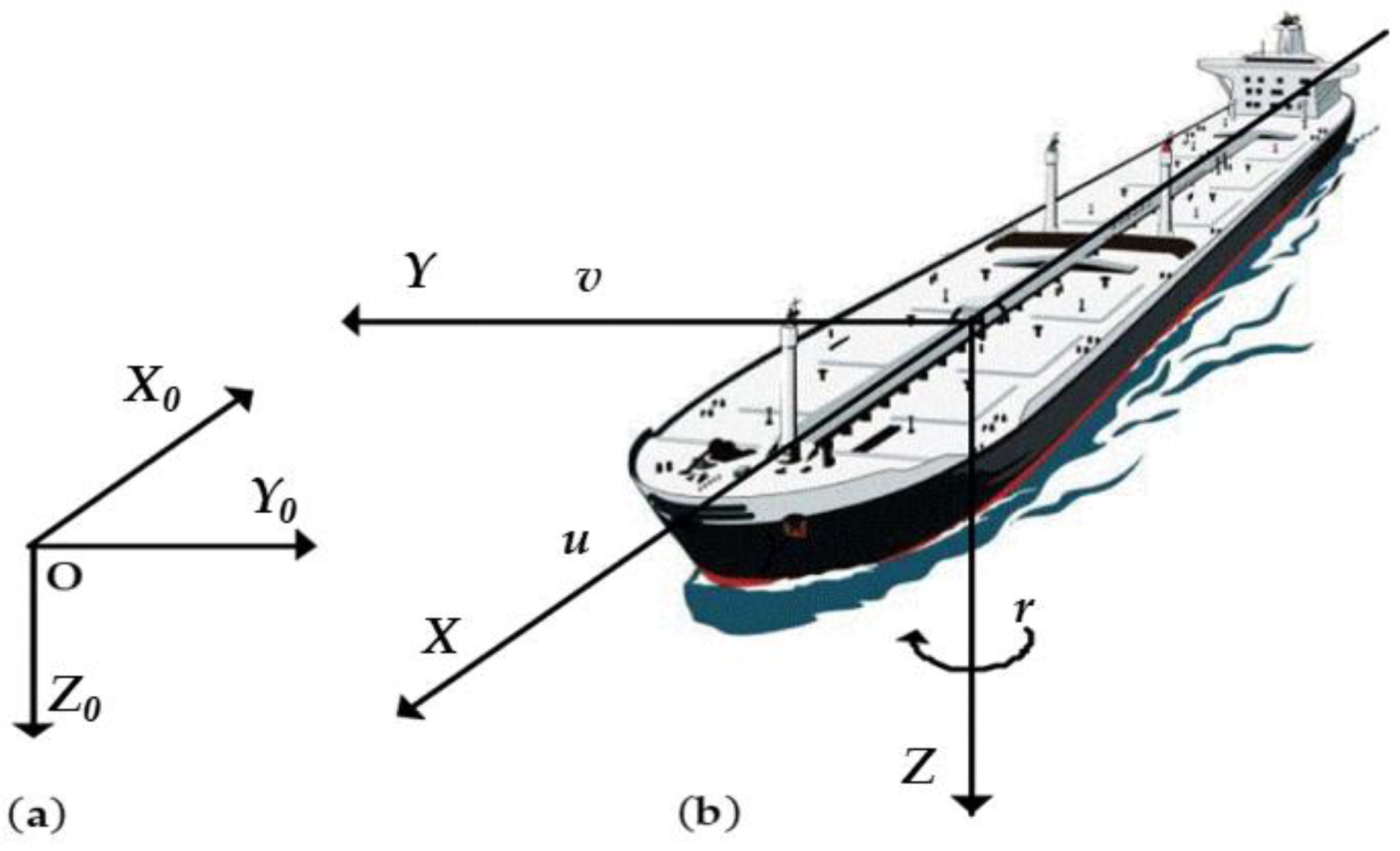
2.2. Coordinate System

The first step in solving the DP problem is to describe the motion of the ship in an appropriate coordinate system. Generally speaking, two coordinate systems are used to describe the motion of the ship, including the North-East-Down (NED) coordinate system $\left(X_0{, Y}_0{, Z}_0\right)$ and the body-fixed coordinate system $\left(X, Y, Z\right)$. The two coordinate systems are shown in Figure 2 [28].

The NED coordinate system is a coordinate system based on the earth. Its origin O can be selected at any point on the surface of the earth, and its three axes point to north, east and the direction of gravity, respectively. Once determined, the three-axis directions are always maintained constant.

The origin of the body-fixed coordinate system is located at the center of gravity of the ship: its horizontal axis X is parallel to the hull and points to the forward direction; the longitudinal axis Y is perpendicular to the hull and points to the starboard side of the hull; the axis Z is same as the direction of gravity and points to the direction of the keel.

2.3. Mathematical Model of the Ship

The mathematical models of ship motion include the kinematic model and the dynamic model. The actual motion of the ship is extremely complex, and generally has six Degrees of Freedom (DOF). The mathematical model proposed by T.I. Fossen in [29] is used to model the ship motion in this study.

2.3.1. Kinematic Model

For marine ships, six DOF models are often used to describe the motion of ships. These six DOF are named surge, sway, heave, roll, pitch and yaw. The vector $\mathsf{\eta }$ consists of the position components and angle component of the marine ships. The vector $\mathsf{\nu }$ consists of the linear speed components and angular speed component of the marine ships. The vectors can be described as follows:

$$\begin{array}{l}{\mathsf{\eta }=[x y z \phi \theta \psi ]}^{\mathrm{T}},{\mathsf{\eta }}_{\mathbf{1}}{=[x y z]}^{\mathrm{T}}, {\mathsf{\eta }}_{\mathbf{2}}{=[\phi \theta \psi ]}^{\mathrm{T}};\\ {\mathsf{\nu }=[u v w p q r]}^{\mathrm{T}}, {\mathsf{\nu }}_{\mathbf{1}}{=[u v w]}^{\mathrm{T}}, {\mathsf{\nu }}_{\mathbf{2}}{=[p q r]}^{\mathrm{T}}.\end{array}$$

The kinematic model of ships is shown in Equation (1):

$$\left\{\begin{array}{c}{\dot{\mathsf{\eta }}}_{\mathbf{1}}{=\mathbf{J}}_{\mathbf{1}}\left(\mathsf{\eta }\right){\mathsf{\nu }}_{\mathbf{1}}\\ {\dot{\mathsf{\eta }}}_{\mathbf{2}}{\mathbf{=}\mathbf{J}}_{\mathbf{2}}\left(\mathsf{\eta }\right){\mathsf{\nu }}_{\mathbf{2}}\end{array}\right.$$

(1)

The ${\mathsf{J}}_{\mathbf{1}}\left(\mathsf{\eta }\right)$ and ${\mathbf{J}}_{\mathbf{2}}\left(\mathsf{\eta }\right)$ are rotation matrices:

$${\mathbf{J}}_{\mathbf{1}}\left(\mathsf{\eta }\right)=\left[\begin{array}{ccc}\cos \theta \cos \psi & \cos \psi \sin \theta \sin \phi -\cos \phi \sin \psi & \sin \psi \sin \phi +\cos \psi \cos \phi \sin \theta \\ \cos \theta \sin \psi & \sin \psi \sin \theta \sin \phi +\cos \phi \cos \psi & -\cos \psi \sin \phi +\sin \psi \cos \phi \sin \theta \\ -\sin \theta & \cos \theta \sin \phi & \cos \theta \cos \phi \end{array}\right],$$

$${\mathbf{J}}_{\mathbf{2}}\left(\mathsf{\eta }\right)=\left[\begin{array}{ccc}1& \sin \phi \tan \theta & \cos \phi \tan \theta \\ 0& \cos \phi & -\sin \phi \\ 0& \sin \phi /\cos \theta & \cos \phi /\cos \theta \end{array}\right].$$

So Equation (1) can be expressed as Equation (2):

$$\left[\begin{array}{c}{\dot{\mathsf{\eta }}}_{\mathbf{1}}\\ {\dot{\mathsf{\eta }}}_{\mathbf{2}}\end{array}\right]=\left[\begin{array}{cc}{\mathbf{J}}_{\mathbf{1}}\left(\mathsf{\eta }\right)& {\mathbf{0}}_{\mathbf{3}\mathit{\times }\mathbf{3}}\\ {\mathbf{0}}_{\mathbf{3}\mathit{\times }\mathbf{3}}& {\mathbf{J}}_{\mathbf{2}}\left(\mathsf{\eta }\right)\end{array}\right]\left[\begin{array}{c}{\mathsf{\nu }}_{\mathbf{1}}\\ {\mathsf{\nu }}_{\mathbf{2}}\end{array}\right]$$

(2)

For general surface vessels, the six DOF can be simplified to three DOF including surge, sway and yaw because vessels always travel at a low speed. In this case, $\phi$ and $\theta$ are very small and can be neglected. It is a good approximate expression for most conventional ships and offshore platforms [30,31]. Therefore, the rotation matrices can be expressed as:

$${\mathbf{J}}_{\mathbf{1}}\left(\mathsf{\eta }\right)\approx \left[\begin{array}{ccc}\cos \psi & -\sin \psi & 0\\ \sin \psi & \cos \psi & 0\\ 0& 0& 1\end{array}\right], {\mathbf{J}}_{\mathbf{2}}\left(\mathsf{\eta }\right)\approx {\mathrm{I}}_{3\mathit{\times }3}$$

Therefore, the kinematic model of ships with three DOF can be rewritten as:

$$\left[\begin{array}{c}\dot{x}\\ \dot{y}\\ \dot{\psi }\end{array}\right]=\left[\begin{array}{ccc}\cos \psi & -\sin \psi & 0\\ \sin \psi & \cos \psi & 0\\ 0& 0& 1\end{array}\right]\left[\begin{array}{c}u\\ v\\ r\end{array}\right]$$

(3)

That is:

$$\dot{\mathsf{\eta }}=\mathbf{J}\left(\psi \right)\mathsf{\nu }$$

(4)

where

$$\mathbf{J}\left(\psi \right)=\left[\begin{array}{ccc}\cos \psi & -\sin \psi & 0\\ \sin \psi & \cos \psi & 0\\ 0& 0& 1\end{array}\right].$$

In the kinematic model (4), the simplified vector $\mathsf{\eta }={\left[\begin{array}{ccc}x& y& \psi \end{array}\right]}^{\mathrm{T}}$ denotes the ship position $\left(x,y\right)$ and yaw component $\psi$ in the earth fixed coordinate system. The simplified vector ν $={\left[\begin{array}{ccc}u& v& r\end{array}\right]}^{\mathrm{T}}$ denotes the ship linear speed (surge: $u$, sway: $v$) and angular speed $r$ (yaw component).

$\mathbf{J}\left(\psi \right)$ is the rotation matrix between earth fixed frame and body-fixed frame, which is nonsingular for all $\psi$ and has the following property: ${\mathbf{J}}^{\mathbf{-}\mathbf{1}}\left(\psi \right){=\mathbf{J}}^{\mathbf{T}}\left(\psi \right)$ [32].

2.3.2. Dynamic Model

The rigid body dynamic equation can be expressed in the following form:

$$\mathbf{M}\dot{\mathsf{\nu }}+\mathbf{C}\mathbf{(}\mathsf{\nu }\mathbf{)}\mathsf{\nu }+\mathbf{D}\mathbf{(}\mathsf{\nu }\mathbf{)}\mathsf{\nu }=\mathsf{\tau }+\mathbf{a}$$

(5)

In the dynamic model (5), $\mathbf{M}$ is the total inertia matrix including additional mass, which can be expressed as:

$$\mathbf{M}=\left[\begin{array}{ccc}\mathrm{m}-{\mathrm{X}}_{\dot{u}}& 0& 0\\ 0& \mathrm{m}-{\mathrm{Y}}_{\dot{v}}& {\mathrm{mx}}_{\mathrm{g}}-{\mathrm{Y}}_{\dot{r}}\\ 0& {\mathrm{mx}}_{\mathrm{g}}-{\mathrm{N}}_{\dot{v}}& {\mathrm{I}}_{\mathrm{zz}}-{\mathrm{N}}_{\dot{r}}\end{array}\right]$$

(6)

The matrix $\mathbf{M}$ can be expressed as ${\mathbf{M}=\mathbf{M}}_{\mathbf{A}}{+\mathbf{M}}_{\mathbf{RB}}$. ${\mathbf{M}}_{\mathbf{A}}$ is the inertia matrix of the hydrodynamic system and ${\mathbf{M}}_{\mathbf{RB}}$ is the inertia matrix of the rigid body system (platform or vessel).

$\mathbf{C}\left(\mathsf{\nu }\right)$ is the Coriolis-centripetal force matrix. Generally, in the case of low-speed motion, the Coriolis-centripetal force matrix $\mathbf{C}\left(\mathsf{\nu }\right)$ is very small and can be neglected, namely $\mathbf{C}\left(\mathsf{\nu }\right)\approx 0$.

$\mathbf{D}\left(\mathsf{\nu }\right)$ is the damping matrix which the surge mode can be decoupled from steering modes (sway and yaw). Therefore, the linearized damping matrix can be written:

$$\mathbf{D}\left(\mathsf{\nu }\right)=\left[\begin{array}{ccc}-{\mathrm{X}}_u& 0& 0\\ 0& -{\mathrm{Y}}_v& -{\mathrm{Y}}_r\\ 0& -{\mathrm{N}}_v& -{\mathrm{N}}_r\end{array}\right]$$

(7)

The damping coefficients can be considered linear in the case of low-speed operation which means that ${\mathrm{N}}_v\mathit{=}{\mathrm{Y}}_r$ such that ${\mathbf{D}}^{\mathbf{T}}=\mathbf{D}$ [29].

The vector $\mathsf{\tau }=[\mathrm{Fx} \mathrm{Fy} \mathrm{Fn}]$ represents the total thrust forces and moment generated by thrusters. The term $\mathbf{a}$ is used to represent the external environmental disturbance forces and moments.

In summary, the three DOF motion mathematical model of the ship can be expressed as a combination of the kinematic model and the dynamic model, as shown in Equation (8) [33]:

$$\left\{\begin{array}{c}\dot{\mathsf{\eta }}=\mathsf{J}\left(\mathbf{\psi }\right)\mathsf{\nu }\\ \mathbf{M}\dot{\mathsf{\nu }}+\mathbf{D}\left(\mathsf{\nu }\right)\mathsf{\nu }=\mathsf{\tau }+\mathbf{a}\end{array}\right.$$

(8)

3. Environmental Disturbances including Wind and Wave

Some experts and scholars have conducted studies on environmental disturbances. Reference [34] predicted for KVLCC2 performing straight ahead motion in head regular waves by using the expanded RANS solver based on OpenFOAM. Reference [35] proposed a numerical model of sea wave generation and a forming filter based on the wave spectrum. This paper adopted external disturbances models from Thor I. Fossen. For control system design it is common to assume the principle of superposition when considering wind and wave disturbances. For most marine control applications this is a good approximation [29]. Environmental disturbances vector $\mathbf{a}$ can be expressed as:

$${\mathbf{a}=\mathbf{a}}_{\mathbf{wind}}{+\mathbf{a}}_{\mathbf{wave}}$$

(9)

${\mathbf{a}}_{\mathbf{wind}}$ means the wind forces and moment vector. ${\mathbf{a}}_{\mathbf{wave}}$ means the waves forces and moment vector.

3.1. Wind Disturbance

The wind speed ${\mathrm{V}}_{\mathrm{T}}$ at any height can be expressed as:

$${\mathrm{V}}_{\mathrm{T}}=\mathrm{V}\ast {(\frac{\mathrm{h}}{10})}^{1/7}$$

(10)

where $\mathrm{V}$ is the average wind speed and h is height.

Relative wind speed ${\mathrm{V}}_{\mathrm{r}}$ can be expressed as:

$${\mathrm{V}}_{\mathrm{r}}{=\mathrm{V}}_{\mathrm{T}}^2{+\mathrm{V}}_{\mathrm{S}}^2{+2\mathrm{V}}_{\mathrm{T}}{\mathrm{V}}_{\mathrm{S}}{\cos (\mathsf{\phi }}_{\mathrm{wind}}-{\mathsf{\phi }}_{\mathrm{ship}}+\mathsf{\gamma })$$

(11)

where ${\mathrm{V}}_{\mathrm{s}}$ is the speed of ship, ${\mathsf{\phi }}_{\mathrm{wind}}$ is the wind direction, ${\mathsf{\phi }}_{\mathrm{ship}}$ is the ship direction and $\mathsf{\gamma }$ is the drift angle.

The generalized wind force vector is ${\mathbf{a}}_{\mathbf{wind}}{=[\mathrm{X}}_{\mathrm{wind}}{,\mathrm{Y}}_{\mathrm{wind}}{,\mathrm{N}}_{\mathrm{wind}}]$. The wind disturbance models in this paper proposed by Isherwood [36] are expressed in Equation (12):

$$\{\begin{array}{c}{\mathrm{X}}_{\mathrm{wind}}=0{.5\mathrm{C}}_{\mathrm{X}}{\mathsf{\rho }}_{\mathsf{\alpha }}{\mathrm{V}}_{\mathrm{r}}^2{\mathrm{A}}_{\mathrm{T}}\\ {\mathrm{Y}}_{\mathrm{wind}}=0{.5\mathrm{C}}_{\mathrm{Y}}{\mathsf{\rho }}_{\mathsf{\alpha }}{\mathrm{V}}_{\mathrm{r}}^2{\mathrm{A}}_{\mathrm{L}}\\ {\mathrm{N}}_{\mathrm{wind}}=0{.5\mathrm{C}}_{\mathrm{N}}{\mathsf{\rho }}_{\mathsf{\alpha }}{\mathrm{V}}_{\mathrm{r}}^2{\mathrm{LA}}_{\mathrm{L}}\end{array}$$

(12)

where ${\mathrm{C}}_{\mathrm{X}}$ and ${\mathrm{C}}_{\mathrm{Y}}$ are the empirical force coefficients, ${\mathrm{C}}_{\mathrm{N}}$ is a moment coefficient, which can be obtained by regression analysis. ${\mathsf{\rho }}_{\mathsf{\alpha }}$ is the density of air, ${\mathrm{A}}_{\mathrm{T}}$ and ${\mathrm{A}}_{\mathrm{L}}$ are the transverse and lateral projected areas, and $\mathrm{L}$ is the overall length of the ship.

3.2. Wave Disturbance

The wave force can be divided into first-order wave force and second-order wave force. The first-order wave force is often ignored due to its small effect. The second-order wave force can be considered to be generated by the wave spectra. This paper adopts Pierson-Moskowitz Spectrum (PM Spectrum) to model the wave, which is shown as:

$$\mathrm{S}\left({\mathsf{\omega }}_{\mathrm{i}}\right)=0{.0081\mathrm{g}}^2{\mathsf{\omega }}_{\mathrm{i}}^{-5}\exp (-\frac{3.11}{{\mathrm{H}}_{\mathrm{s}}^2}{\mathsf{\omega }}_{\mathrm{i}}^{-4})$$

(13)

where $\mathrm{g}$ is gravitational acceleration, ${\mathsf{\omega }}_{\mathrm{i}}$ is the wave frequency of the i-th wave and ${\mathrm{H}}_{\mathrm{s}}$ is wave height.

The waves force vector is ${\mathbf{a}}_{\mathbf{wave}}=[{\mathrm{X}}_{\mathrm{wave}},{\mathrm{Y}}_{\mathrm{wave}},{\mathrm{N}}_{\mathrm{wave}}]$. The wave disturbance can be expressed as follows:

$$\{\begin{array}{c}{\mathrm{X}}_{\mathrm{wave}}=-0{.5\mathsf{\rho }\mathrm{L}\mathsf{\mu }}^2{\cos \mathsf{\chi }\mathrm{C}}_{\mathrm{XW}}\\ {\mathrm{Y}}_{\mathrm{wave}}=0{.5\mathsf{\rho }\mathrm{L}\mathsf{\mu }}^2{\sin \mathsf{\chi }\mathrm{C}}_{\mathrm{YW}}\\ {\mathrm{N}}_{\mathrm{wave}}=0{.5\mathsf{\rho }\mathrm{L}}^2{\mathsf{\mu }}^2{\sin \mathsf{\chi }\mathrm{C}}_{\mathrm{NW}}\end{array}$$

(14)

where $\mathsf{\chi }$ is encounter angle and $\mathsf{\mu }$ is wave amplitude. ${\mathrm{C}}_{\mathrm{XW}}$, ${\mathrm{C}}_{\mathrm{YW}}$ and ${\mathrm{C}}_{\mathrm{NW}}$ are coefficients obtained by regression analysis.

In this paper, the fourth-level sea state is taken into account as environmental disturbances, which have 2 m wave height and 10 m/s average wind speed.

4. ADRC Ship DP Controller

The control objective of the system modeling is to find a control law such that the actual position and trajectory can converge to a desired position and trajectory.

4.1. Basic Principle of ADRC

Deriving Equation (8) allows to establish Equation (15):

$$\ddot{\mathsf{\eta }}=\dot{\mathbf{J}}\mathsf{\nu }-{\mathbf{JM}}^{\mathbf{-}\mathbf{1}}{\mathbf{D}\mathsf{\nu }+\mathbf{JM}}^{\mathbf{-}\mathbf{1}}{\mathbf{a}+\mathbf{JM}}^{\mathbf{-}\mathbf{1}}\mathsf{\tau }$$

(15)

By setting ${\mathbf{x}}_1=\mathsf{\eta }$ and ${\mathbf{x}}_{\mathbf{2}}=\dot{\mathsf{\eta }}$, a state space model of the ship can be obtained from Equation (15) as follows:

$$\left\{\begin{array}{c}{\dot{\mathbf{x}}}_{\mathbf{1}}={\mathbf{x}}_2\\ {\dot{\mathbf{x}}}_{\mathbf{2}}=\mathbf{f}\left({\mathbf{x}}_{\mathbf{1}}{\mathbf{,}\mathbf{x}}_2\mathbf{,}\mathbf{t}\right)+\mathsf{\omega }\left(\mathbf{t}\right)+\mathrm{b}\mathbf{u}\\ {\mathbf{y}=\mathbf{x}}_{\mathbf{1}}\end{array}\right.$$

(16)

where ${\mathbf{u}=\mathbf{JM}}^{\mathbf{-}\mathbf{1}}\mathsf{\tau }$ is the control quantity, ${\mathsf{\omega }\left(\mathbf{t}\right)=\mathbf{JM}}^{\mathbf{-}\mathbf{1}}\mathbf{a}$ is the unknown disturbance and $\mathbf{f}({\mathbf{x}}_{\mathbf{1}}\mathbf{,}{\mathbf{x}}_{\mathbf{2}}\mathbf{,}\mathbf{t})=\dot{\mathbf{J}}\mathsf{\nu }\mathbf{-}{\mathbf{JM}}^{\mathbf{-}\mathbf{1}}\mathbf{D}\mathsf{\nu }$ is the known disturbance. $\mathbf{y}$ is the output and $\mathrm{b}$ is the control gain.

Due to the good decoupling performance of ADRC, a single dimension is considered in the following part to simplify analysis. The control analysis of this system is described as follows:

Step 1: Arranging the transition process.

In classical control, $\dot{\mathsf{\eta }}=\frac{\mathsf{\eta }\left(\mathrm{t}\right)-\mathsf{\eta }(\mathrm{t}-\mathrm{T})}{\mathrm{T}}$ is generally used to generate differential signals. The smaller $\mathrm{T}$ is, the closer the output is to the differential signal. However, if $\mathrm{T}$ is too small, this process may result in the amplification of noise effects. Therefore, it is necessary to take a suitable method to extract the differential signal.

For the system shown below, it is hoped that ${\mathsf{\eta }}_1$ can be asymptotically stable at the target ${\mathsf{\eta }}_0$ and ${\mathsf{\eta }}_2$ can be asymptotically stable at the differential of the target. The algorithm formula is as follows:

$$\left\{\begin{array}{c}{\dot{\mathsf{\eta }}}_1{=\mathsf{\eta }}_1+\mathrm{h}\ast {\mathsf{\eta }}_2\\ {\dot{\mathsf{\eta }}}_2{=\mathsf{\eta }}_2+\mathrm{h}\ast \mathsf{\Gamma }\end{array}\right.$$

(17)

$\mathsf{\Gamma }$ is a control law which can be taken as a sign function or a sat function (a saturation function). However, the two functions will produce high-frequency noise when the system enters a steady state. Hence, this paper adopts fst function to design the fastest discrete feedback system. The specific expression of $\mathrm{fst}$ function is [37]:

$$\{\begin{array}{c}{\mathrm{d}=\mathrm{r}}_0\ast {\mathrm{h}}_0\\ {\mathrm{d}}_0=\mathrm{d}\ast {\mathrm{h}}_0\\ {\mathrm{y}=\mathsf{\eta }}_1{+\mathrm{h}}_0\ast {\mathsf{\eta }}_2\\ {\mathsf{\alpha }}_0=\sqrt{{\mathrm{d}}^2{+8\mathrm{r}}_0\left|\mathrm{y}\right|}\\ \mathsf{\alpha }=\{\begin{array}{c}{\mathsf{\eta }}_2+\frac{{(\mathsf{\alpha }}_0-\mathrm{d}\left)\mathrm{sign}\right(\mathrm{y})}{2}{,\left|\mathrm{y}\right|>\mathrm{d}}_0\\ {\mathsf{\eta }}_2+\frac{\mathrm{y}}{{\mathrm{h}}_0},\left|\mathrm{y}\right|\le {\mathrm{d}}_0\end{array}\\ \mathrm{fst}=\{\begin{array}{c}-\frac{{\mathrm{r}}_0\ast \mathsf{\alpha }}{\mathrm{d}},\left|\mathsf{\alpha }\right|\le \mathrm{d}\\ -{\mathrm{r}}_0\ast \mathrm{sign}\left(\mathsf{\alpha }\right),\left|\mathsf{\alpha }\right|>\mathrm{d}\end{array}\end{array}$$

(18)

Equation (18) is the fastest synthesis function, which can be obtained by the ‘Isochronic Region method’. Due to the complexity of derivation process, the specific derivation process and variable meanings can be learned in reference [38] written by Prof. Han. In the Equation (18), ${\mathrm{r}}_0$ is the factor of tracking speed and ${\mathrm{h}}_0$ is filter factor that represents filter effect. For the speed factor ${\mathrm{r}}_0$, the value should not be too large or too small. If the value is too small, the tracking speed is too slow, while if the value is too large, the differential signal is poor when the given signal will be noisy.

Therefore, transition process can be designed as Equation (19) and then the tracking signal ${\mathsf{\eta }}_1$ and differential signal ${\mathsf{\eta }}_2$ can be obtained according to the given input signal ${\mathsf{\eta }}_0$. This module can be called Tracking Differentiator (TD). The specific algorithm formula is shown in Equation (19):

$$\left\{\begin{array}{c}{\dot{\mathsf{\eta }}}_1{=\mathsf{\eta }}_1+\mathrm{h}\ast {\mathsf{\eta }}_2\\ {\dot{\mathsf{\eta }}}_2{=\mathsf{\eta }}_2+\mathrm{h}\ast {\mathrm{fst}(\mathsf{\eta }}_1-{\mathsf{\eta }}_0{,\mathsf{\eta }}_2{,\mathrm{r}}_0{,\mathrm{h}}_0)\end{array}\right.$$

(19)

where $\mathrm{fst}(·)$ is the modified fastest synthesis function. ${\mathsf{\eta }}_1$ is the tracking signal and the ${\mathsf{\eta }}_2$ is the differential signal. h is the sample step time. For the step h, the value should not be too small, otherwise the differential performance will not be guaranteed. The value of the step h can generally be chosen in the (0.001, 0.1) range.

Step 2: Estimating the state of each order of the controlled system.

The total disturbance $\mathrm{f}\left({\mathrm{x}}_1{,\mathrm{x}}_2,\mathrm{t}\right)+\mathsf{\omega }\left(\mathrm{t}\right)$ in the second-order ship system (16) is expanded into a new state variable $\mathrm{f}$. Then state equation of the system can be expressed as:

$$\left\{\begin{array}{c}{\dot{\mathrm{x}}}_1{=\mathrm{x}}_2\\ {\dot{\mathrm{x}}}_2=\mathrm{f}+\mathrm{bu}\\ \dot{\mathrm{f}}={\mathsf{\omega }}_0\left(\mathrm{t}\right)\\ {\mathrm{y}=\mathrm{x}}_1\end{array}\right.$$

(20)

For such a system, the state observer can be expressed as:

$$\left\{\begin{array}{c}\mathrm{e}={\widehat{\mathsf{\eta }}}_1-\mathsf{\eta }\\ {\dot{\widehat{\mathsf{\eta }}}}_1={\widehat{\mathsf{\eta }}}_2-{\mathsf{\beta }}_{01}\ast \mathrm{e}\\ {\dot{\widehat{\mathsf{\eta }}}}_2=\widehat{\mathrm{f}}-{\mathsf{\beta }}_{02}\ast {\left|\mathrm{e}\right|}^{0.5}\mathrm{sign}\left(\mathrm{e}\right)+\mathrm{b}\ast \mathrm{u}\\ \dot{\widehat{\mathrm{f}}}=-{\mathsf{\beta }}_{03}\ast {\left|\mathrm{e}\right|}^{0.25}\mathrm{sign}\left(\mathrm{e}\right)\end{array}\right.$$

(21)

where ${\widehat{\mathsf{\eta }}}_1$, ${\widehat{\mathsf{\eta }}}_2$, $\widehat{\mathrm{f}}$ are the estimations of ${\mathrm{x}}_1$, ${\mathrm{x}}_2$, $\mathrm{f}$, respectively. ${\mathsf{\beta }}_{01}$, ${\mathsf{\beta }}_{02}$, ${\mathsf{\beta }}_{03}$ are adjustable parameters whose values should be greater than 0. The three parameters determine the effect of estimating the disturbances and have a mutually restrictive relationship, the ideal estimation effect of which can be obtained by coordination action. Hence, as long as the appropriate ${\mathsf{\beta }}_{01}$, ${\mathsf{\beta }}_{02}$ and ${\mathsf{\beta }}_{03}$ are selected, the system can estimate the state variables ${\mathrm{x}}_1$, ${\mathrm{x}}_2$ and $\mathrm{f}$, namely ${\widehat{\mathsf{\eta }}}_1\to {\mathrm{x}}_1$, ${\widehat{\mathsf{\eta }}}_2\to {\mathrm{x}}_2$ and $\widehat{\mathrm{f}}\to \mathrm{f}$.

In order to avoid the phenomenon of high-frequency flutter, ${\left|\mathrm{e}\right|}^{0.5}\mathrm{sign}\left(\mathrm{e}\right)$ and ${\left|\mathrm{e}\right|}^{0.25}\mathrm{sign}\left(\mathrm{e}\right)$ need to be transformed into a nonlinear function which is continuous around the origin. The fal function was therefore proposed by Han in [39]. Its expression is shown as follows:

$$\mathrm{fal}\left(\mathrm{e},\mathsf{\alpha },\mathsf{\delta }\right)=\{\begin{array}{c}{\left|\mathrm{e}\right|}^{\mathsf{\alpha }}\mathrm{sign}\left(\mathrm{e}\right),\left|\mathrm{e}\right|>\mathsf{\delta }\\ \frac{\mathrm{e}}{{\mathsf{\delta }}^{1-\mathsf{\alpha }}},\left|\mathrm{e}\right|\le \mathsf{\delta }\end{array}$$

(22)

Fal function is a nonlinear function that has fast convergence which can be referred to in Section 5.2.1. $\mathsf{\delta }$ is a small number greater than 0 and $\mathsf{\alpha }$ is a parameter that determines the shape of the fal function. This parameter is chosen in (0, 1) range.

According to the input u and output η of the system, the observer can be designed as shown in Equation (23):

$$\left\{\begin{array}{c}\mathrm{e}={\widehat{\mathsf{\eta }}}_1-\mathsf{\eta }\\ {\dot{\widehat{\mathsf{\eta }}}}_1={\widehat{\mathsf{\eta }}}_2-{\mathsf{\beta }}_{01}\ast \mathrm{e}\\ {\dot{\widehat{\mathsf{\eta }}}}_2=\widehat{\mathrm{f}}-{\mathsf{\beta }}_{02}\ast \mathrm{fal}\left({\mathrm{e},\mathsf{\alpha }}_1,\mathsf{\delta }\right)+\mathrm{b}\ast \mathrm{u}\\ \dot{\widehat{\mathrm{f}}}=-{\mathsf{\beta }}_{03}\ast \mathrm{fal}\left({\mathrm{e},\mathsf{\alpha }}_2,\mathsf{\delta }\right)\end{array}\right.$$

(23)

where $\mathrm{b}$ is control coefficient. ${\mathsf{\beta }}_{01}$, ${\mathsf{\beta }}_{02}$, ${\mathsf{\beta }}_{03}$ are adjustable parameters greater than 0.

This observer is called Extended State Observer (ESO) and the control effect of the system depends on the observation of the total disturbances by ESO.

Step 3: Non-linear combination and the compensation of total disturbance.

The control variable u of classical control is usually a linear combination of the error related to present (e(t)), past (${{\displaystyle \int }}_0^{\mathrm{t}}\mathrm{e}\left(\mathrm{t}\right)\mathrm{dt}$) and future ($\frac{\mathrm{de}\left(\mathrm{t}\right)}{\mathrm{dt}}$). However, such a combination is not necessarily applicable in a large number of engineering practices. Therefore, ADRC uses the fal function mentioned before to change the linear combination into the nonlinear combination. The non-linear combination is called Non-linear State Error Feedback (NLSEF) and its expression is shown in Equation (24):

$$\left\{\begin{array}{c}{\mathrm{e}}_1={\mathsf{\eta }}_1-{\widehat{\mathsf{\eta }}}_1\\ {\mathrm{e}}_2={\mathsf{\eta }}_2-{\widehat{\mathsf{\eta }}}_2\\ {\mathrm{u}}_0{=\mathrm{k}}_1\ast \mathrm{fal}\left({\mathrm{e}}_1{,\mathsf{\alpha }}_{\mathrm{n}1},\mathsf{\delta }\right){+\mathrm{k}}_2\ast \mathrm{fal}\left({\mathrm{e}}_2{,\mathsf{\alpha }}_{\mathrm{n}2},\mathsf{\delta }\right)\\ {\mathrm{u}=\mathrm{u}}_0-\widehat{\mathrm{f}}/\mathrm{b}\end{array}\right.$$

(24)

where ${\mathrm{k}}_1$ and ${\mathrm{k}}_2$ are adjustable parameters. As long as the parameters of fal function and ${\mathrm{k}}_1$ and ${\mathrm{k}}_2$ are selected appropriately, it can ensure that the controller may have good robustness and adaptability.

4.2. Stability Analysis of Control System

Rewrite the state space form of the second-order controlled ship system in this paper as follows:

$$\left\{\begin{array}{c}{\dot{\mathrm{x}}}_1{=\mathrm{x}}_2\\ {\dot{\mathrm{x}}}_2=\mathrm{f}+\mathrm{bu}\\ {\mathrm{y}=\mathrm{x}}_1\end{array}\right.$$

(25)

To simplify the analysis of the problem, this paper uses the following assumptions:

(1)

Set ${\mathrm{z}}_1={\widehat{\mathsf{\eta }}}_1$, ${\mathrm{z}}_2={\widehat{\mathsf{\eta }}}_2$ and ${\mathrm{z}}_3=\widehat{\mathrm{f}}$. The three variables are the estimations of tracking signal, differential signal and total disturbances, respectively.

(2)

Let the input be 0, then the output of TD is also 0.

(3)

Change the Nonlinear State Error Feedback (NLSEF) into Linear State Error Feedback (LSEF):

$${\mathrm{u}=\mathrm{k}}_1{\mathrm{z}}_1{+\mathrm{k}}_2{\mathrm{z}}_2-\frac{{\mathrm{z}}_3}{\mathrm{b}}$$

(26)

(4)

Select nonlinear function $\mathsf{\phi }\left(\mathrm{x}\right)$ which satisfies that if $\mathrm{x}\ne 0$, then $\mathrm{x}\mathsf{\phi }\left(\mathrm{x}\right)>0$. Define $\mathsf{\phi }\in \mathrm{F}\left({\mathsf{\varsigma }}_1{,\mathsf{\varsigma }}_2\right)$ to satisfy the following conditions: ①$\mathsf{\phi }\left(0\right)=0$; ②${\mathsf{\varsigma }}_1{\mathrm{x}}^2<\mathrm{x}\mathsf{\phi }\left(\mathrm{x}\right){<\mathsf{\varsigma }}_2{\mathrm{x}}^2 \left(\forall \mathrm{x}\ne 0\right)$ and then $\mathrm{x}\mathsf{\phi }\left(\mathrm{x}\right)>0$, namely $\mathsf{\phi }\in \mathrm{F}\left(0,\infty \right)$.

$$\left\{\begin{array}{c}{\dot{\mathrm{z}}}_1{=\mathrm{z}}_2-{\mathsf{\beta }}_{01}\mathsf{\phi }\left({\mathrm{z}}_1-\mathrm{y}\right)\\ {\dot{\mathrm{z}}}_2{=\mathrm{z}}_3-{\mathsf{\beta }}_{02}\mathsf{\phi }\left({\mathrm{z}}_1-\mathrm{y}\right)+\mathrm{bu}\\ {\dot{\mathrm{z}}}_3=-\mathsf{\phi }\left({\mathrm{z}}_1-\mathrm{y}\right)\end{array}\right.$$

(27)

(5)

Let the control object be a linear time-invariant object:

$$\left\{\begin{array}{c}\ddot{\mathrm{x}}=-{\mathrm{a}}_2\mathrm{x}-{\mathrm{a}}_1\dot{\mathrm{x}}+\mathrm{bu}\\ \mathrm{y}=\mathrm{x}\end{array}\right.$$

(28)

Substituting Equation (26) and Equation (28) into Equation (25) can get:

$$\left\{\begin{array}{c}\dot{\mathbf{X}}={\mathbf{A}}_{\mathrm{11}}\mathbf{X}+{\mathbf{A}}_{\mathbf{12}}\mathbf{Z}+{\mathbf{a}}_{\mathbf{13}}{\mathbf{z}}_{\mathbf{3}}\\ {\mathrm{y}=\mathrm{x}}_1\end{array}\right.$$

(29)

where $\mathbf{X}={\left[{\mathrm{x}}_1{, \mathrm{x}}_2\right]}^{\mathrm{T}}$, ${\mathbf{Z}=[\mathrm{z}}_1{,\mathrm{z}}_2{]}^{\mathrm{T}}$, ${\mathbf{a}}_{\mathbf{13}}=[0, -{1]}^{\mathrm{T}}$, ${\mathbf{A}}_{\mathbf{11}}=\left[\begin{array}{cc}0& 1\\ -{\mathrm{a}}_2& -{\mathrm{a}}_1\end{array}\right]$, ${\mathbf{A}}_{\mathbf{12}}=\left[\begin{array}{cc}0& 0\\ {\mathrm{bk}}_1& {\mathrm{bk}}_2\end{array}\right]$.

Substitute Equation (26) into Equation (27) to get:

$$\left\{\begin{array}{c}\dot{\mathbf{Z}}={\mathbf{A}}_{\mathbf{22}}\mathbf{Z}+{\mathbf{b}}_{\mathbf{2}}\mathsf{\zeta }\\ {\dot{\mathrm{z}}}_3{=\mathsf{\beta }}_{03}\mathsf{\zeta }\\ \mathsf{\zeta }=-\mathsf{\phi }\left({\mathrm{z}}_1-\mathrm{y}\right)\end{array}\right.$$

(30)

where ${\mathbf{b}}_{\mathbf{2}}{=[\mathsf{\beta }}_{01}{, \mathsf{\beta }}_{02}{]}^{\mathrm{T}}$, ${\mathbf{A}}_{\mathbf{22}}=\left[\begin{array}{cc}0& 1\\ {\mathrm{bk}}_1& {\mathrm{bk}}_2\end{array}\right]$.

Combine Equation (29) and Equation (30) can get:

$$\left\{\begin{array}{c}\dot{\mathbf{X}}={\mathbf{A}}_{\mathrm{11}}\mathbf{X}+{\mathbf{A}}_{\mathbf{12}}\mathbf{Z}+{\mathbf{a}}_{\mathbf{13}}{z}_3\\ \dot{\mathbf{Z}}={\mathbf{A}}_{\mathbf{22}}\mathbf{Z}+{\mathbf{b}}_{\mathbf{2}}\mathsf{\zeta }\\ {\dot{\mathrm{z}}}_3{=\mathsf{\beta }}_{03}\mathsf{\zeta }\\ \mathsf{\zeta }=-\mathsf{\phi }\left(\mathsf{\theta }\right)\\ {\mathsf{\theta }=\mathbf{c}}_{\mathbf{1}}^{\mathbf{T}}{\mathbf{X}+\mathbf{c}}_2^{\mathbf{T}}\mathbf{Z}\end{array}\right.$$

(31)

where ${\mathbf{c}}_{\mathbf{1}}=[-{1, 0]}^{\mathrm{T}}$, ${\mathbf{c}}_{\mathbf{2}}{=[1, 0]}^{\mathrm{T}}$.

Let ${\mathbf{Y}=\mathbf{A}}_{\mathbf{11}}{\mathbf{X}+\mathbf{a}}_{\mathbf{13}}{\mathrm{z}}_3$, ${\mathrm{z}}_3^{\prime }{=\mathrm{z}}_3{/\mathsf{\beta }}_{03}$ and Equation (32) can be available after arranging the equation:

$$\left\{\begin{array}{c}\dot{\mathbf{Y}}={\mathbf{A}}_{\mathbf{11}}\mathbf{Y}+{\mathbf{A}}_{\mathbf{11}}{\mathbf{A}}_{\mathbf{12}}\mathbf{Z}+{\mathbf{a}}_{\mathbf{13}}{\mathsf{\beta }}_{03}\mathsf{\zeta }\\ \dot{{Z}}={\mathbf{A}}_{\mathbf{22}}\mathbf{Z}+{\mathbf{b}}_{\mathbf{2}}\mathsf{\zeta }\\ {\dot{\mathrm{z}}}_3={\mathsf{\beta }}_{03}\mathsf{\zeta }\\ \mathsf{\zeta }=-\mathsf{\phi }\left(\mathsf{\theta }\right)\\ {\mathsf{\theta }=\mathbf{c}}_{\mathbf{1}}^{\mathbf{T}}{\mathbf{A}}_{\mathbf{11}}^{\mathbf{-}\mathbf{1}}{\mathbf{Y}+\mathbf{c}}_{\mathbf{2}}^{\mathbf{T}}\mathbf{Z}-{\mathbf{c}}_{\mathbf{1}}^{\mathbf{T}}{\mathbf{A}}_{\mathbf{11}}^{\mathbf{-}\mathbf{1}}{\mathbf{a}}_{\mathbf{13}}{\mathsf{\beta }}_{03}{\mathrm{z}}_3^{\prime }\end{array}\right.$$

(32)

That is:

$$\left\{\begin{array}{c}\left[\begin{array}{c}\dot{\mathbf{Y}}\\ \dot{\mathbf{Z}}\end{array}\right]=\left[\begin{array}{cc}{\mathbf{A}}_{\mathbf{11}}& {\mathbf{A}}_{\mathbf{11}}{\mathbf{A}}_{\mathbf{12}}\\ \mathbf{0}& {\mathbf{A}}_{\mathbf{22}}\end{array}\right]\left[\begin{array}{c}\mathbf{Y}\\ \mathbf{Z}\end{array}\right]+\left[\begin{array}{c}{\mathbf{a}}_{\mathbf{13}}{\mathsf{\beta }}_{03}\\ {\mathbf{b}}_{\mathbf{2}}\end{array}\right]\mathsf{\zeta }\\ {\dot{\mathrm{z}}}_3{=\mathsf{\beta }}_{03}\mathsf{\zeta }\\ \mathsf{\zeta }=-\mathsf{\phi }\left(\mathsf{\theta }\right)\\ \mathsf{\theta }=[\begin{array}{cc}{\mathbf{c}}_{\mathbf{1}}^{\mathbf{T}}{\mathbf{A}}_{\mathbf{11}}^{\mathbf{-}\mathbf{1}}& {\mathbf{c}}_{\mathbf{2}}^{\mathbf{T}}]\end{array}\left[\begin{array}{c}\mathbf{Y}\\ \mathbf{Z}\end{array}\right]-{\mathbf{c}}_{\mathbf{1}}^{\mathbf{T}}{\mathbf{A}}_{\mathbf{11}}^{\mathbf{-}\mathbf{1}}{\mathbf{a}}_{\mathbf{13}}{\mathrm{z}}_3\end{array}\right.$$

(33)

Equation (33) conforms to a standard form of the first critical case of absolute stability, which is:

$$\left\{\begin{array}{c}\dot{\mathrm{x}}=\mathbf{A}\mathrm{x}+\mathbf{b}\mathrm{u}\\ \dot{\mathsf{\xi }}=\mathrm{u}\\ \mathrm{u}=-\mathsf{\phi }\left(\mathrm{y}\right)\\ {\mathrm{y}=\mathrm{c}}^{\mathrm{T}}\mathrm{x}+\mathsf{\rho }\mathsf{\xi }\end{array}\right.$$

(34)

where $\mathbf{A}=\left[\begin{array}{cc}{\mathbf{A}}_{\mathbf{11}}& {\mathbf{A}}_{\mathbf{11}}{\mathbf{A}}_{\mathbf{12}}\\ 0& {\mathbf{A}}_{\mathbf{22}}\end{array}\right]$, $\mathbf{b}=\left[\begin{array}{c}{\mathbf{a}}_{\mathbf{13}}{\mathsf{\beta }}_{03}\\ {\mathbf{b}}_{\mathbf{2}}\end{array}\right]$, ${\mathbf{c}}^{\mathbf{T}}=[\begin{array}{cc}{\mathbf{c}}_{\mathbf{1}}^{\mathbf{T}}{\mathbf{A}}_{\mathbf{11}}^{\mathbf{-}\mathbf{1}}& {\mathbf{c}}_{\mathbf{2}}^{\mathbf{T}}\end{array}]$, $\mathsf{\rho }=-{\mathbf{c}}_{\mathbf{1}}^{\mathbf{T}}{\mathbf{A}}_{\mathbf{11}}^{\mathbf{-}\mathbf{1}}{\mathbf{a}}_{\mathbf{13}}$.

Theorem 1.

The necessary condition for the absolute stability of the zero solution of $F\mathit{\left(}0\mathit{,}\mathit{\infty }\mathit{\right)}$in System (34) is$\mathit{Re}\mathit{\left[}\lambda \mathit{\left(}\mathit{A}\mathit{\right)}\mathit{\right]}\mathit{<}0\mathit{,} \rho \mathit{>}0\mathit{,}$[40].

We can construct a Lyapunov function:

$$\mathrm{V}\left(\mathrm{x},\mathrm{y}\right){=\mathbf{x}}^{\mathbf{T}}\mathbf{Qx}+ϵ{(\mathrm{y}-{\mathbf{c}}^{\mathbf{T}}\mathbf{x})}^2+\mathsf{\beta }{{\displaystyle \int }}_0^{\mathrm{y}}\mathsf{\phi }\left(\mathrm{y}\right)\mathrm{dy}$$

(35)

If $\mathbf{Q}$ is a positive definite matrix and $ϵ, \mathsf{\beta }\ge 0$, $\mathrm{V}\left(\mathrm{x},\mathrm{y}\right)$ is a positive definite function.

Find the derivative of $\mathrm{V}\left(\mathrm{x},\mathrm{y}\right)$:

$$\begin{gathered} -\dot{\mathrm{V}}(\mathrm{x},\mathrm{y})={\mathbf{x}}^{\mathbf{T}}(-\mathbf{Q}\mathbf{A}-{\mathbf{A}}^{\mathbf{T}}\mathbf{Q})\mathbf{x} \\ \hspace{1em}\hspace{1em}+\left({2\mathbf{b}}^{\mathbf{T}}\mathbf{Q}-2ϵ{\mathsf{\rho }\mathbf{c}}^{\mathbf{T}}-{\mathsf{\beta }\mathbf{c}}^{\mathbf{T}}\mathbf{A}\right)\mathbf{x}\mathsf{\phi }\left(\mathrm{y}\right) \\ \hspace{1em}\hspace{1em}{+(\mathsf{\beta }\mathsf{\rho }+\mathsf{\beta }\mathbf{c}}^{\mathbf{T}}{\mathbf{b})\mathsf{\phi }}^2\left(\mathrm{y}\right)+2ϵ\mathsf{\rho }\mathrm{y}\mathsf{\phi }\left(\mathrm{y}\right) \end{gathered}$$

(36)

Since $\mathrm{y}\mathsf{\phi }\left(\mathrm{y}\right)>0$, $\mathsf{\rho }>0$, as long as $ϵ\ge 0$ and the first three terms of Equation (36) are the positive definite quadratic form, then $\dot{\mathrm{V}}$ must be negative definite, thus ensuring the global asymptotic stability of the system. Therefore, as long as the parameters are properly selected to satisfy the relevant conditions, the stability can be ensured.

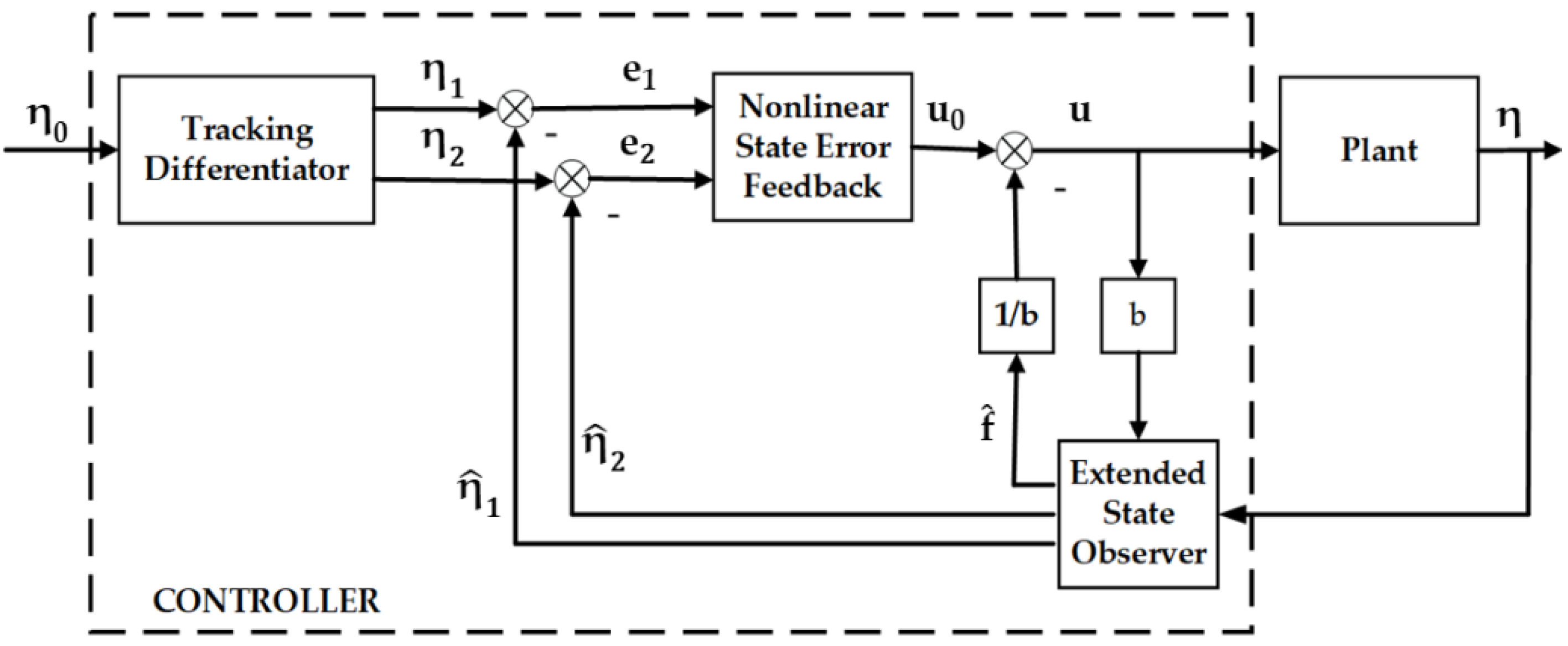
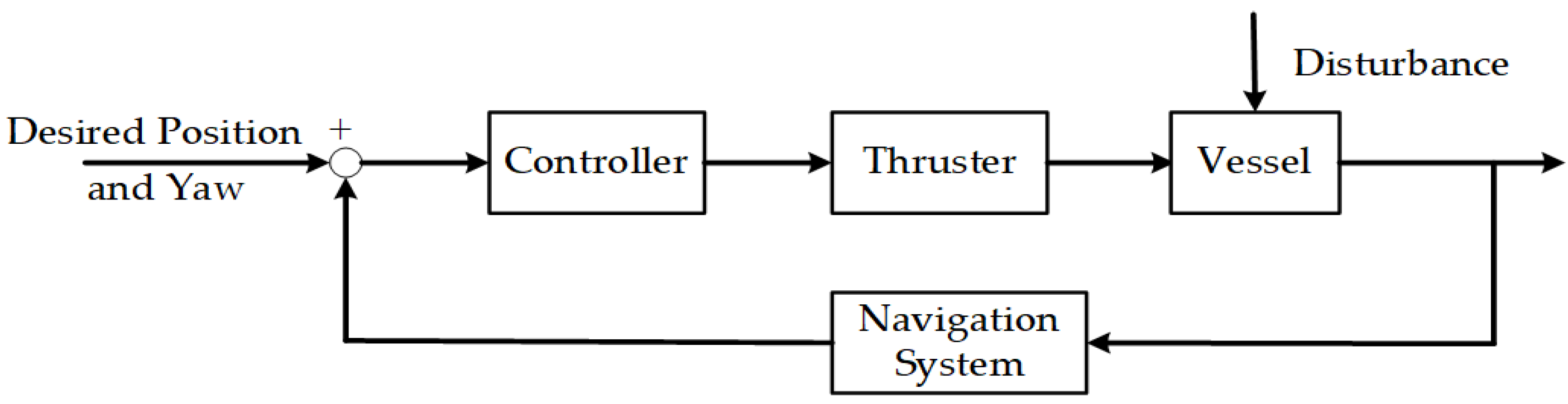
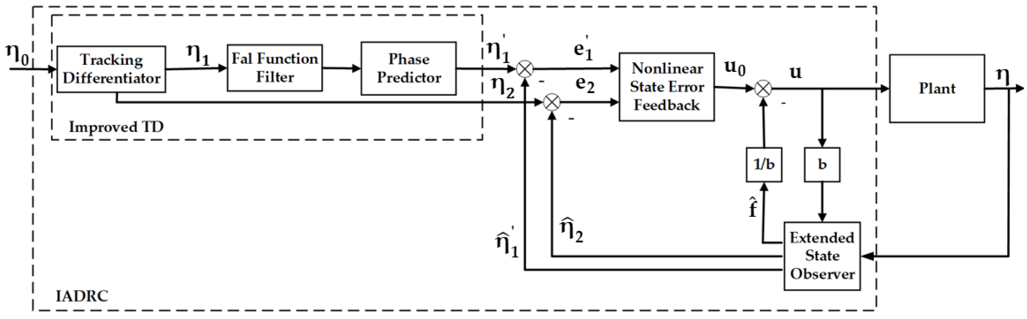
4.3. Structure of ADRC

According to the above analysis, ADRC method of the DP ship can be obtained based on Equations (19), (23) and (24). ADRC is composed of three parts [41]: TD, ESO and NLSEF. The structure of ADRC is shown in Figure 3 [42]. ADRC is a nonlinear control that does not rely on precise mathematical models [43]. It promotes and enriches the error-based idea of classical control and has strong advantages, especially in uncertain models and the ocean environment [44], which has fast speed, strong anti-disturbance ability and good nonlinear control performance.

5. Improvement of ADRC Controller

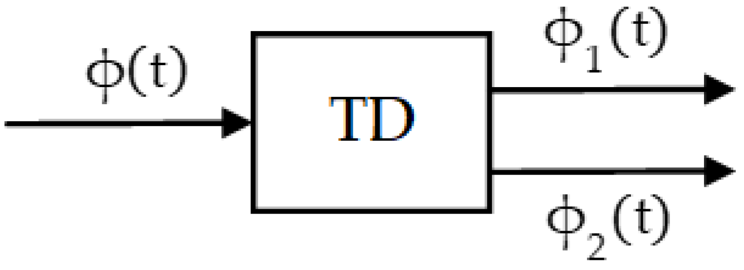
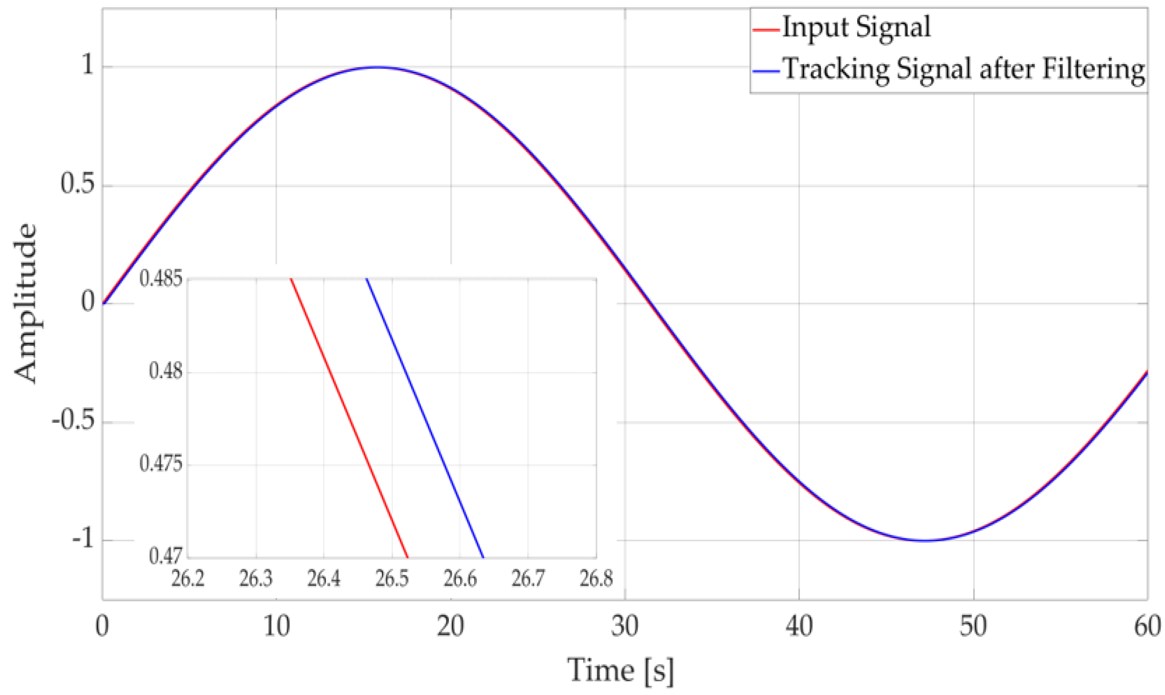
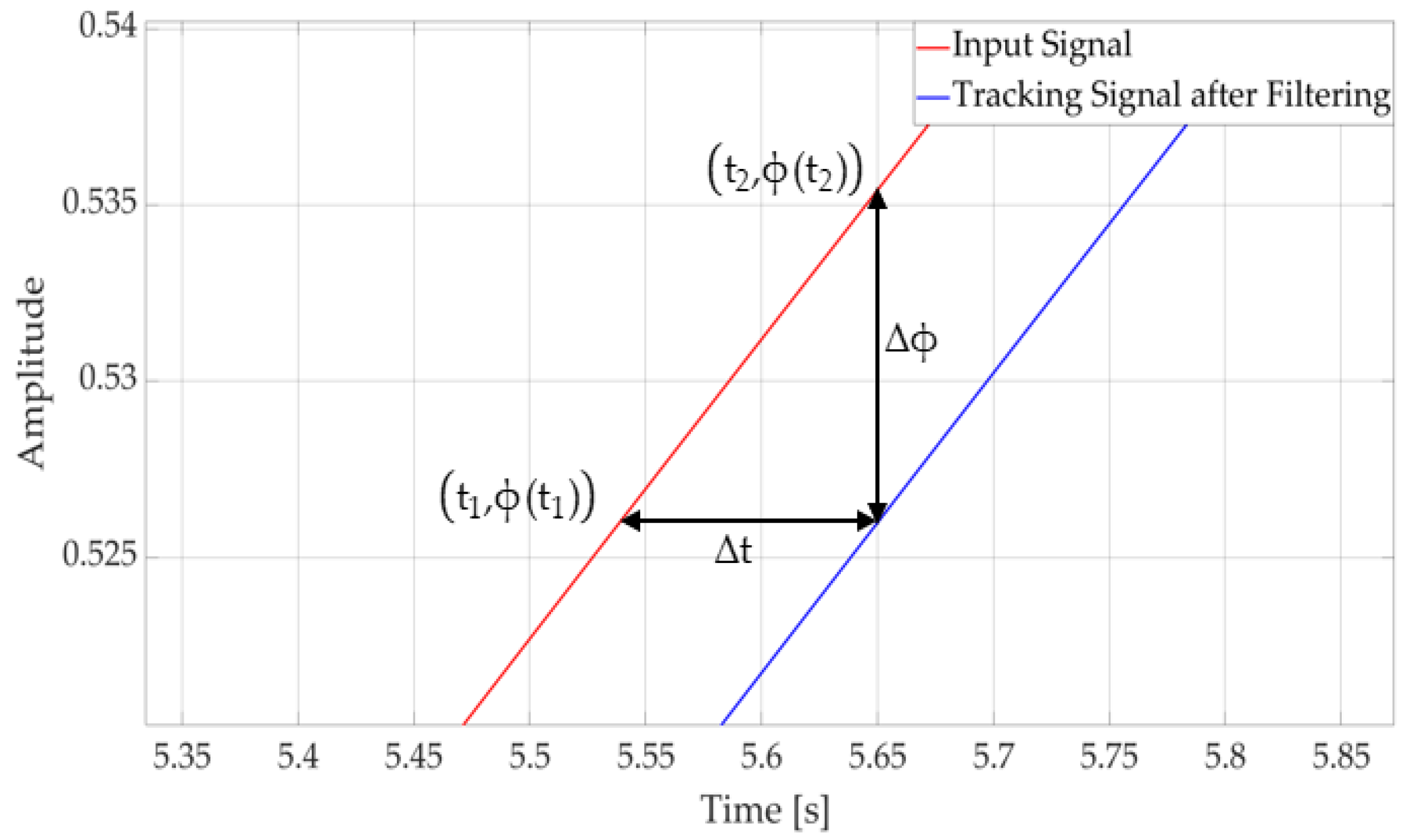
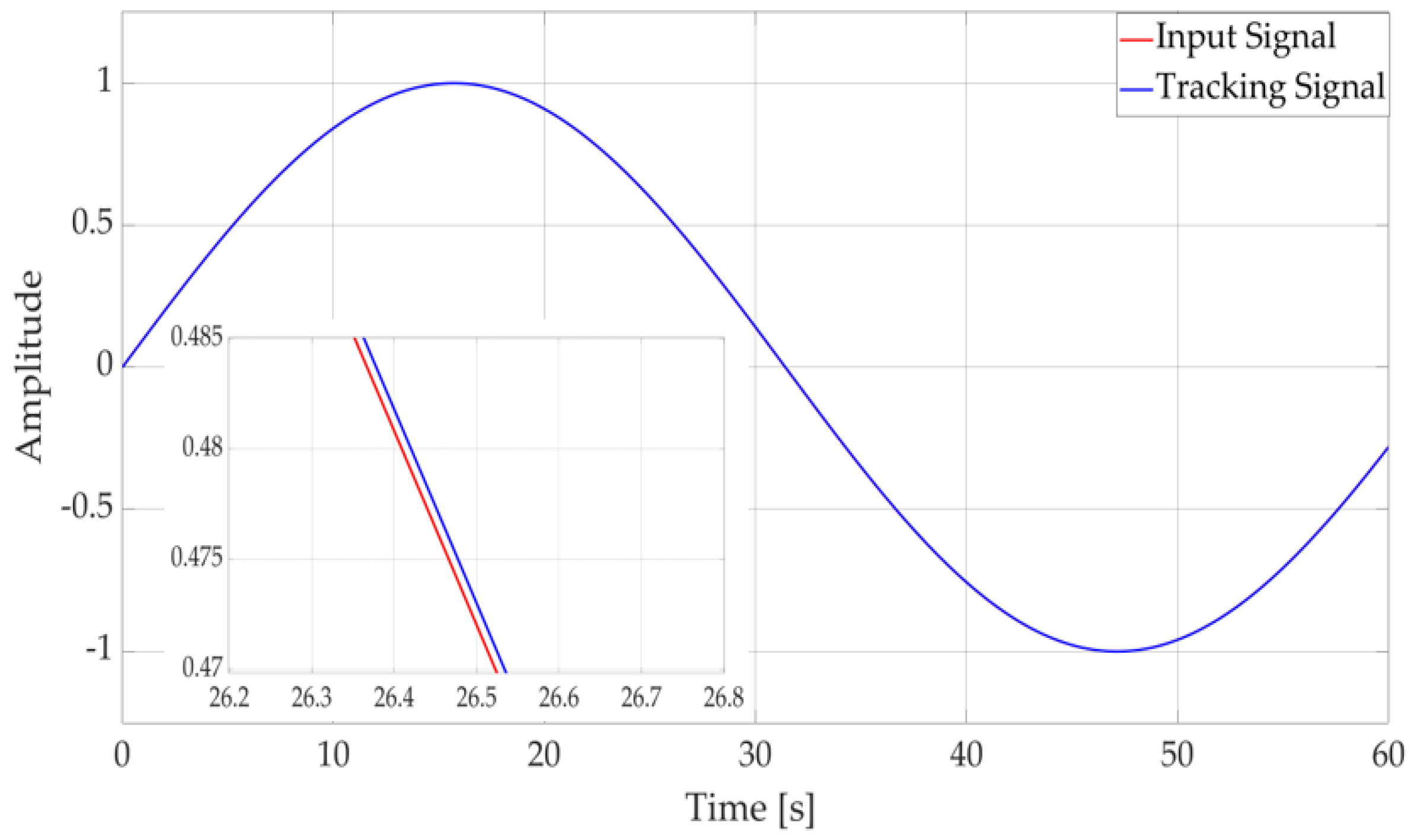
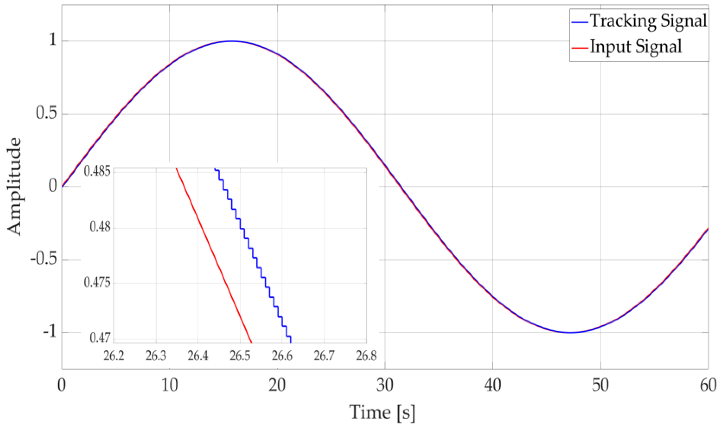
5.1. Analysis of TD Behavior and Limitations

Since ADRC has good decoupling performance and different working conditions have different requirements on the ship’s trajectory, this section only considers the control effect of single control channel to conduct simplified theoretical analysis, which is shown in Figure 4.

This paper assumes that the input reference signal is a sinusoidal signal $\mathsf{\varphi }\left(\mathrm{t}\right)=\sin (0.1\mathrm{t})$ to illustrate the existing problems. The simulation result on TD is shown in Figure 5. The red line is the input signal $\mathsf{\varphi }\left(\mathrm{t}\right)$, and the blue line is the tracking signal ${\mathsf{\varphi }}_1\left(\mathrm{t}\right)$. It is found that the tracking signal ${\mathsf{\varphi }}_1\left(\mathrm{t}\right)$ has a phase delay and dither, which has a great impact on the track control and may cause the tracking error to be non-zero all the time. This error may lead to a decrease in the accuracy of the ship’s DP control, possibly resulting in position deviations in some marine operations such as oil extraction and cable laying. Therefore, this paper adopts an effective method to solve the problems of dither and phase delay to reduce the error of straight track control.

5.2. Improvement Methods

5.2.1. Fal Function Filter

To solve the dithering problem, this paper adopts the fal function filter to eliminate dither. The fal function has good filtering performance and can also solve the dithering problem well. The characteristic analysis of the fal function filter is given below.

The following system is available:

$$\dot{\mathrm{x}}=\mathrm{w}\left(\mathrm{x},\mathrm{t}\right)+\mathrm{s}$$

(37)

where $\mathrm{w}\left(\mathrm{x},\mathrm{t}\right)$ represents environmental disturbances and is less than ${\mathrm{w}}_{\mathrm{d}}$ which is maximum value of external disturbances. The form $\mathrm{s}$ is the control variable.

This paper takes the feedback $\mathrm{s}$ of state $\mathrm{x}$ as $\mathrm{s}=\mathrm{s}\left(\mathrm{x}\right)$.

Let $\mathrm{s}\left(\mathrm{x}\right)=-\mathrm{k}\ast \mathrm{fal}(\mathrm{x}, \mathsf{\alpha }, \mathsf{\delta })$ and then the fal function can be rewritten as follows:

$$\mathrm{fal}\left(\mathrm{x},\mathsf{\alpha },\mathsf{\delta }\right)=\{\begin{array}{c}{\left|\mathrm{x}\right|}^{\mathsf{\alpha }}\mathrm{sign}\left(\mathrm{x}\right),\left|\mathrm{x}\right|>\mathsf{\delta }\\ \frac{\mathrm{x}}{{\mathsf{\delta }}^{1-\mathsf{\alpha }}},\left|\mathrm{x}\right|\le \mathsf{\delta }\end{array},\mathsf{\delta }>0$$

(38)

When $\left|\mathrm{x}\right|>\mathsf{\delta }$, system (37) becomes:

$$\dot{\mathrm{x}}=\mathrm{w}\left(\mathrm{x},\mathrm{t}\right)-\mathrm{k}{\left|\mathrm{x}\right|}^{\mathsf{\alpha }}\mathrm{sign}\left(\mathrm{x}\right)$$

(39)

Multiply both sides by $2\mathrm{x}$ and Equation (40) can be obtained as follows:

$$\frac{\mathrm{d}\left({\mathrm{x}}^2\right)}{\mathrm{dt}}\le -2\mathrm{k}\left|\mathrm{x}\right|({\left|\mathrm{x}\right|}^{\mathsf{\alpha }}-\frac{{\mathrm{w}}_{\mathrm{d}}}{\mathrm{k}})<0$$

(40)

When $|\mathrm{x}\left(\mathrm{t}\right)|>(\frac{{\mathrm{w}}_{\mathrm{d}}}{\mathrm{k}}{)}^{\frac{1}{\mathsf{\alpha }}}$, control variable $\mathrm{s}=-\mathrm{k}{\left|\mathrm{x}\right|}^{\mathsf{\alpha }}\mathrm{sign}\left(\mathrm{x}\right)$ can control the steady error caused by $\mathrm{w}\left(\mathrm{x},\mathrm{t}\right)$ within the range of $\left|\mathrm{x}\right|\le {\left|\frac{{\mathrm{w}}_{\mathrm{d}}}{\mathrm{k}}\right|}^{\frac{1}{\mathsf{\alpha }}}$.

When $\left|\mathrm{x}\right|\le \mathsf{\delta }$, system (37) becomes:

$$\dot{\mathrm{x}}=\mathrm{w}\left(\mathrm{x},\mathrm{t}\right)-\mathrm{k}\frac{\mathrm{x}}{{\mathsf{\delta }}^{1-\mathsf{\alpha }}}$$

(41)

Multiply both sides by $2\mathrm{x}$ and Equation (42) can be obtained as follows:

$$\frac{\mathrm{d}\left({\mathrm{x}}^2\right)}{\mathrm{dt}}\le -{2\mathrm{x}}^2\left(\frac{\mathrm{k}}{{\mathsf{\delta }}^{1-\mathsf{\alpha }}}-\frac{{\mathrm{w}}_{\mathrm{d}}}{\mathrm{x}}\right)<0$$

(42)

When $|\mathrm{x}\left(\mathrm{t}\right)|>\frac{{|\mathrm{w}}_{\mathrm{d}}{|\mathsf{\delta }}^{1-\mathsf{\alpha }}}{\mathrm{k}}$, control variable $\mathrm{s}=-\mathrm{k}{\left|\mathrm{x}\right|}^{\mathsf{\alpha }}\mathrm{sign}\left(\mathrm{x}\right)$ can control the steady error caused by $\mathrm{w}\left(\mathrm{x},\mathrm{t}\right)$ within the range of $\left|\mathrm{x}\right|\le \frac{\left|{\mathrm{w}}_{\mathrm{d}}\right|{\mathsf{\delta }}^{1-\mathsf{\alpha }}}{\mathrm{k}}$.

The feedback structure of fal function filter can be shown in Figure 6 [45]. The formula of this filter can be expressed as [46]:

$$\left\{\begin{array}{c}\dot{\mathrm{q}}=\mathrm{k}\ast \mathrm{fal}(\mathrm{e},\mathsf{\alpha },\mathsf{\delta })\\ \mathrm{e}=\mathrm{p}-\mathrm{q}\\ {\mathrm{p}}_0=\mathrm{q}\end{array}\right.$$

(43)

where $\mathrm{k}$ is the scale factor. $\mathrm{p}$ is the input signal of the filter and ${\mathrm{p}}_0$ is the output of the filter.

This paper analyzes the filter shown in Equation (43).

When $\left|\mathrm{e}\right|>\mathsf{\delta }$, nonlinear feedback $\mathrm{k}\ast {\left|\mathrm{e}\right|}^{\mathsf{\alpha }}\mathrm{sign}\left(\mathrm{e}\right)$ makes the system state rapidly approach the input signal $\mathrm{p}$, so that the error $\mathrm{e}$ approaches $\mathsf{\delta }$.

When $\left|\mathrm{e}\right|\le \mathsf{\delta }$, $\dot{\mathrm{q}}=\mathrm{k}\ast \mathrm{fal}(\mathrm{e},\mathsf{\alpha },\mathsf{\delta })=\mathrm{k}\ast \mathrm{e}/{\mathsf{\delta }}^{1-\mathsf{\alpha }}$ . Set ${\mathrm{k}}_{\mathrm{f}}{=\mathrm{k}/\mathsf{\delta }}^{1-\mathsf{\alpha }}$. In this case, a transfer function from input to output can be obtained in Equation (44):

$$\frac{{\mathrm{p}}_0}{\mathrm{p}}=\frac{{\mathrm{k}}_{\mathrm{f}}/\mathrm{s}}{{1+\mathrm{k}}_{\mathrm{f}}/\mathrm{s}}=\frac{{\mathrm{k}}_{\mathrm{f}}}{{\mathrm{s}+\mathrm{k}}_{\mathrm{f}}}$$

(44)

Equation (44) is actually a low-pass filter. When $\mathrm{k}$ decreases, the bandwidth becomes narrower and the filtering effect may be better.

According to the above analysis, a fal function filter is used at the output of the TD. As shown in Figure 7, the blue signal is the filtered signal. It can be clearly seen that compared with Figure 5, the original dither signal is turned into a smooth signal by the operation of the fal function filter, which solves the dithering problem.

5.2.2. Phase Prediction

As is shown in Figure 8, the phase prediction method is used in this paper to solve the phase delay problem.

In Figure 8, the red signal is the input curve $\mathsf{\varphi }\left(\mathrm{t}\right)$ and the blue one is the tracking curve ${\mathsf{\varphi }}_1\left(\mathrm{t}\right)$.

According to Figure 8, the new tracking curve ${\mathsf{\varphi }}_1^{\prime }\left(\mathrm{t}\right)$ can be expressed as Equation (45):

$${\mathsf{\varphi }}_1^{\prime }\left(\mathrm{t}\right)={\mathsf{\varphi }}_1\left(\mathrm{t}\right)+\mathsf{\Delta }\mathsf{\varphi }$$

(45)

where $\mathsf{\Delta }\mathsf{\varphi }=\mathsf{\varphi }\left({\mathrm{t}}_2\right)-\mathsf{\varphi }\left({\mathrm{t}}_1\right)$.

Considering that ${\mathsf{\varphi }}_2\left(\mathrm{t}\right)$ is the differential signal of the input signal $\mathsf{\varphi }\left(\mathrm{t}\right)$, Equation (46) can be obtained according to the definition of differential:

$${\mathsf{\varphi }}_2\left(\mathrm{t}\right)=\underset{{\mathrm{t}}_2\to {\mathrm{t}}_1}{\lim }\frac{\mathsf{\varphi }\left({\mathrm{t}}_2\right)-\mathsf{\varphi }\left({\mathrm{t}}_1\right)}{{\mathrm{t}}_2-{\mathrm{t}}_1}$$

(46)

When the time interval is small, Equation (46) can be approximately rewritten as:

$$\mathsf{\Delta }\mathsf{\varphi }{=(\mathrm{t}}_2-{\mathrm{t}}_1){\mathsf{\varphi }}_2\left(\mathrm{t}\right)$$

(47)

Then Equation (45) can be rewritten as:

$${\mathsf{\varphi }}_1^{\prime }\left(\mathrm{t}\right)={\mathsf{\varphi }}_1{\left(\mathrm{t}\right)+(\mathrm{t}}_2-{\mathrm{t}}_1){\mathsf{\varphi }}_2\left(\mathrm{t}\right)$$

(48)

where ${\mathrm{t}}_2-{\mathrm{t}}_1=\mathsf{\lambda }\ast \mathrm{h}$. h is the step time in the tracking differentiator parameters, ${\mathsf{\lambda }=2\ast \mathrm{r}}_1=2\ast \frac{{\mathrm{h}}_0}{\mathrm{h}}$ is the compensation coefficient and ${\mathrm{h}}_0$ is the filter factor which represents the filter effect.

Then the new tracking signal ${\mathsf{\varphi }}_1^{\prime }\left(\mathrm{t}\right)$ can be expressed as:

$${\mathsf{\varphi }}_1^{\prime }\left(\mathrm{t}\right)={\mathsf{\varphi }}_1\left(\mathrm{t}\right)+\mathsf{\lambda }\ast \mathrm{h}\ast {\mathsf{\varphi }}_2\left(\mathrm{t}\right)$$

(49)

The meaning of Equation (49) is that the new tracking signal of the input signal is taken as the original tracking signal plus the product of the differential signal and the predicted step size.

The input signal is already defined above. The simulation result is shown in Figure 9. It can be seen that the error between the input signal and the tracking signal is significantly reduced compared with Figure 7, indicating that the phase prediction method can well overcome the phase delay problem of the tracking differentiator.

The two improvements are applied to design an IADRC to the straight track control. The principle of IADRC is shown in Figure 10.

6. Simulation and Analysis

During the dynamic positioning and tracking process of the ship, the controller calculates the corresponding thrust according to the deviation between the set position and the current position and transmits it to the ship to drive the ship [47]. The ship then feeds the position information back to the controller through the navigation system to form a closed control loop. The control structure of DP system is shown in Figure 11 [48].

Since the ship system in this paper is a coupled MIMO system, ADRC has good decoupling performance. It means that ADRC can be designed separately for each control channel [49]. Therefore, the surge, sway and yaw can be controlled separately in the following study in this paper.

To verify the performance of the controller designed above, a case study ship is used. Its parameters are shown in

Table 1. Parameters of the example ship.

Entry	Data
Ship Length	76.2 m
Ship Width	18.8 m
Ship Height	82.5 m
Draft	6.25 m
Displacement	4200 t
Power	3533 kW

and the mass matrix and damping matrix of the ship follow [50].

The mass matrix and damping matrix of the ship are as follows:

$$\mathrm{M}=\left[\begin{array}{ccc}1.1274& 0& 0\\ 0& 1.8902& -0.0744\\ 0& -0.0744& 0.1278\end{array}\right], \mathrm{D}=\left[\begin{array}{ccc}0.0358& 0& 0\\ 0& 0.1183& -0.0124\\ 0& -0.0041& 0.0308\end{array}\right].$$

The focus of this paper is to improve the structure of ADRC to achieve the control effect. Therefore, parameter tuning of ADRC is not involved in this paper and the parameters of the controllers in this paper are empirical parameters. The automatic adjustment of parameters will be studied in detail in the future.

6.1. Fixed-Point Control and Yaw Control Based on Classical ADRC

To solve the problems of large overshoot, long response time and low positioning accuracy, this paper uses firstly classical ADRC to verify the fixed-point control and yaw control of the ship compared with classical backstepping control.

In the late 1980s, the idea of backstepping was initiated. Some scholars proposed a backstepping design method based on Lyapunov stability for partially linear strict feedback systems [51]. The idea of backstepping control is to divide the entire design process into multiple steps and each step is designed with virtual control and stabilization functions. Then, the control starts from the lowest-order equation of the system, gradually recurses to higher-order equations, and finally realizes the global adjustment of the system. The control structure composed of multiple subsystems can effectively control the n-order nonlinear system. Therefore, the backstepping method has a certain representativeness. The idea of dynamic positioning backstepping controller can be found in the Reference [52].

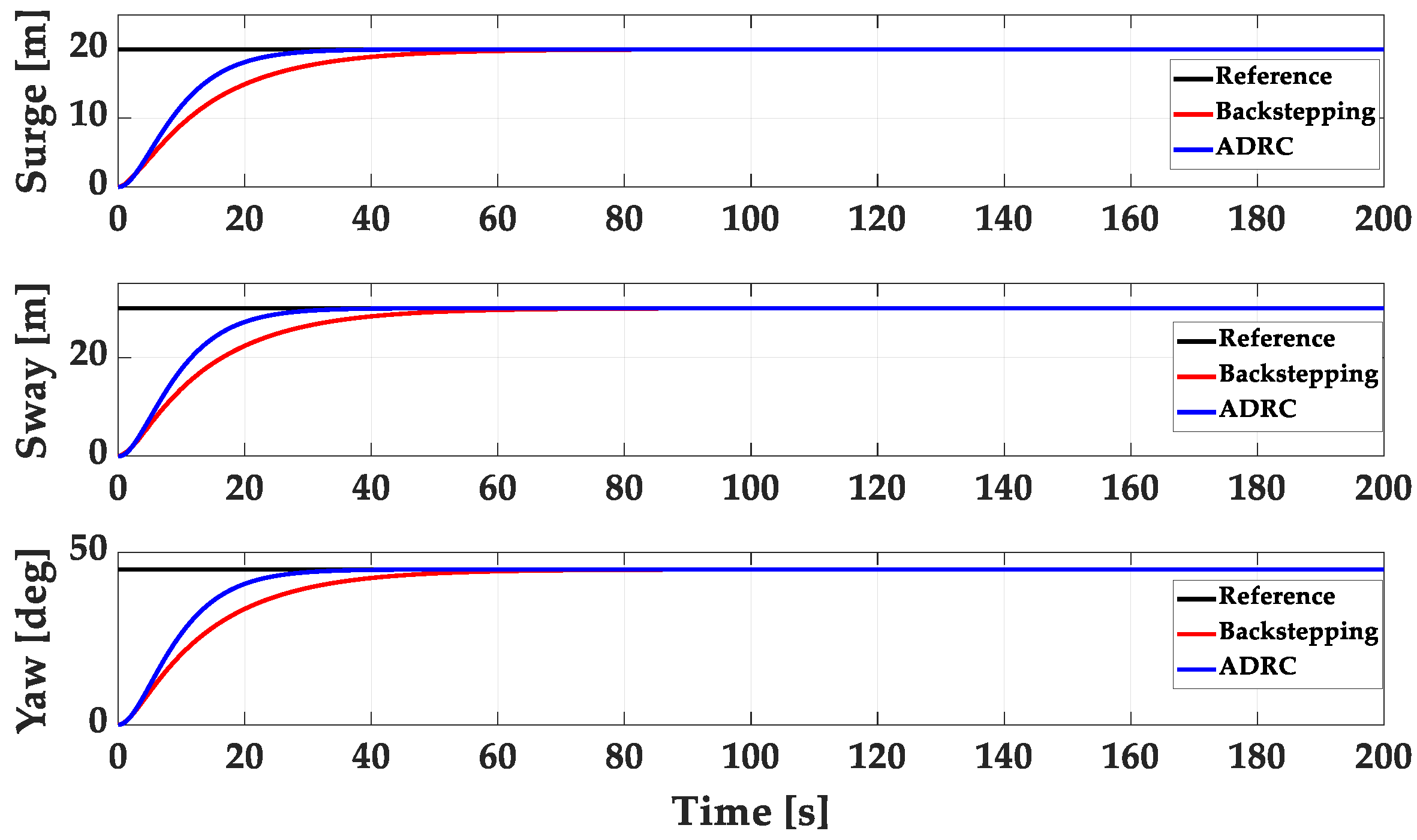
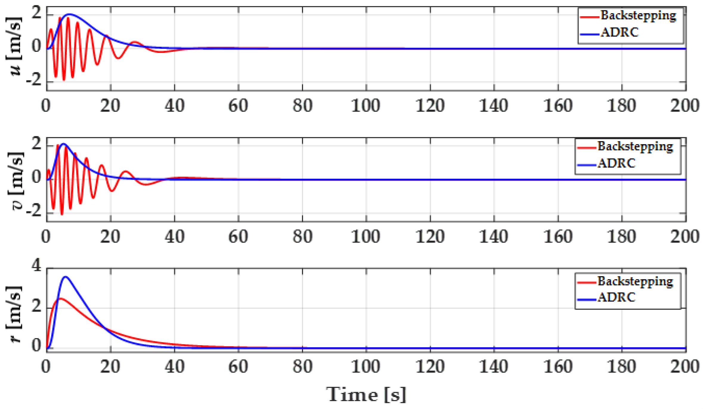
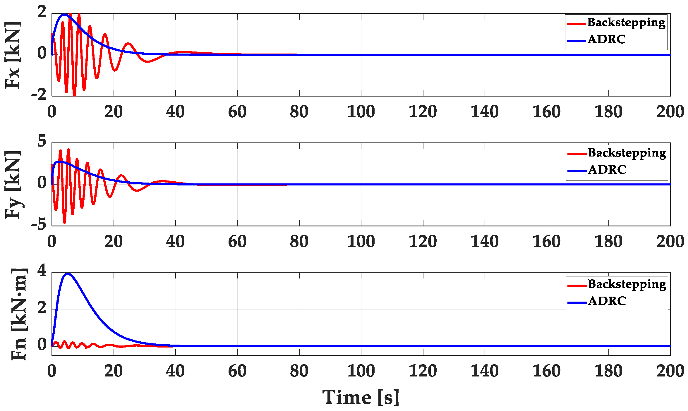
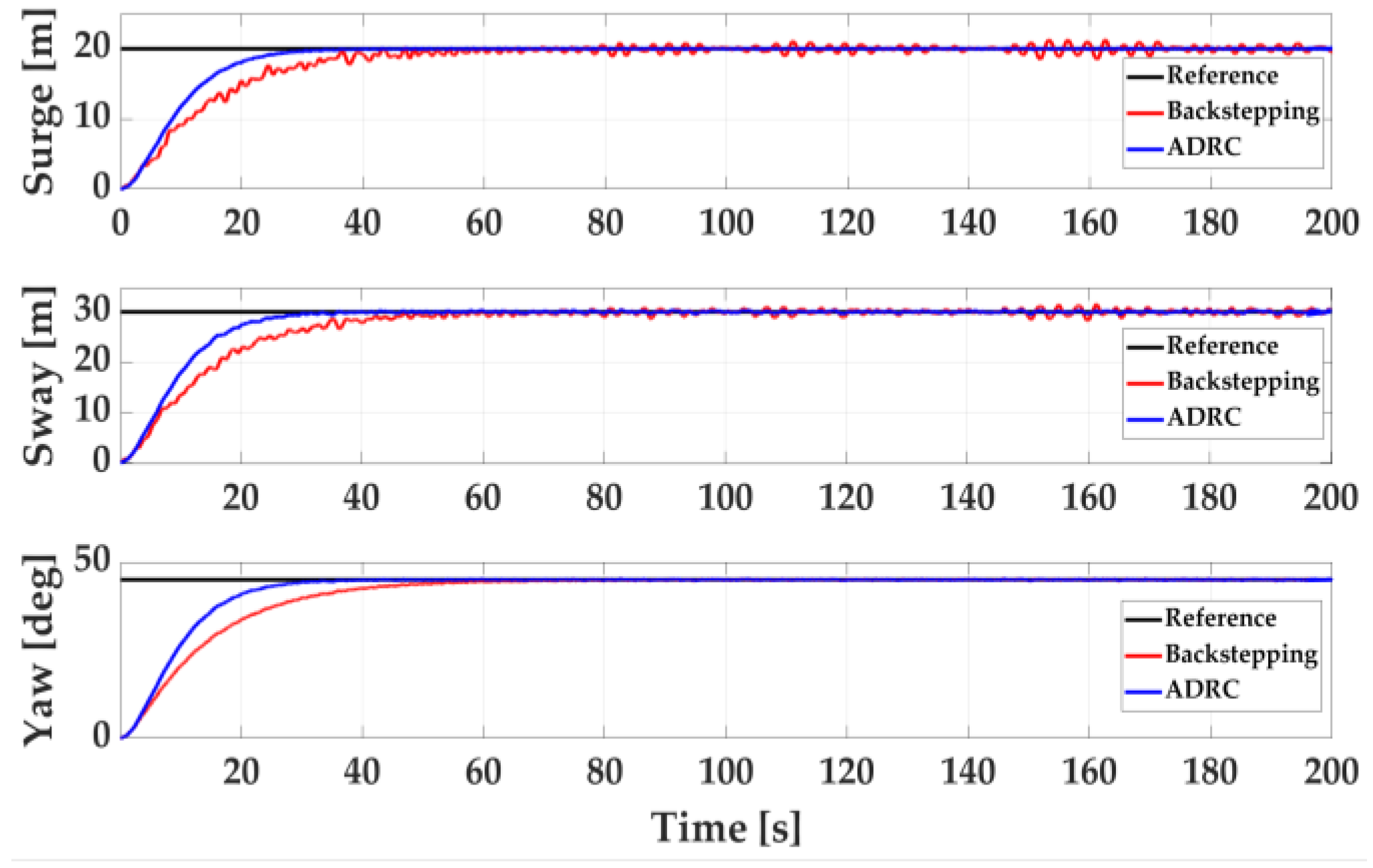
6.1.1. Simulation under Ideal Sea Condition

Firstly, the fixed-point control and yaw control under ideal sea condition are considered. In the simulation, the initial position signal and yaw signal of the ship are set as ${\mathsf{\eta }}_0{=[0 \mathrm{m} 0 \mathrm{m} 0°]}^{\mathrm{T}}$, and the desired target position and yaw signal are set as ${\mathsf{\eta }}_{\mathrm{d}}{=[20 \mathrm{m} 30 \mathrm{m} 45°]}^{\mathrm{T}}$. The simulation time is 200 s. The surge, sway, yaw and position under ideal sea condition can be seen in Figure 12 and Figure 13, respectively. The speed of the ship is shown in Figure 14. The forces and moment of thrusters are shown in Figure 15.

It is obvious from Figure 12 and Figure 13 that both controllers can bring the ship to the set position without overshooting. After reaching the desired position, the ship remains berthed, and the yaw angle reaches the predetermined angle and remains constant. However, ADRC takes about 30 s, while backstepping control takes about 50 s, indicating that the designed ADRC controller can effectively solve the problem of long response time compared with backstepping control. It can be seen from Figure 14 that the linear speed in the surge and sway directions and the angular speed in the yaw direction of the ship with ADRC have large accelerations at the start, and then gradually decelerate. The linear speed in the surge and sway directions of the ship with backstepping control fluctuates greatly in the early stage, and the largest fluctuation is about 2 m/s. The angular speed in the yaw direction of that is consistent with the trend of ADRC, but its maximum speed is only about 2.5 m/s and the deceleration is more stable. After the ship reaches the specified position, the speed decreases to 0 and stays parked. Figure 15 shows the forces and moments of the two controllers. It can be seen that the oscillations of the forces in surge and sway direction in the early stage of backstepping method are more obvious which may cause damage to thrusters and do not exceed about 2 kN and 5 kN. The yaw moment of the backstepping method is much smaller than that of the ADRC, but there is still a small oscillation. The above results prove that the two controllers can both realize fixed-point control and yaw control under ideal sea condition, but according to the comprehensive analysis of position, speed and forces, the performance of ADRC is better than backstepping.

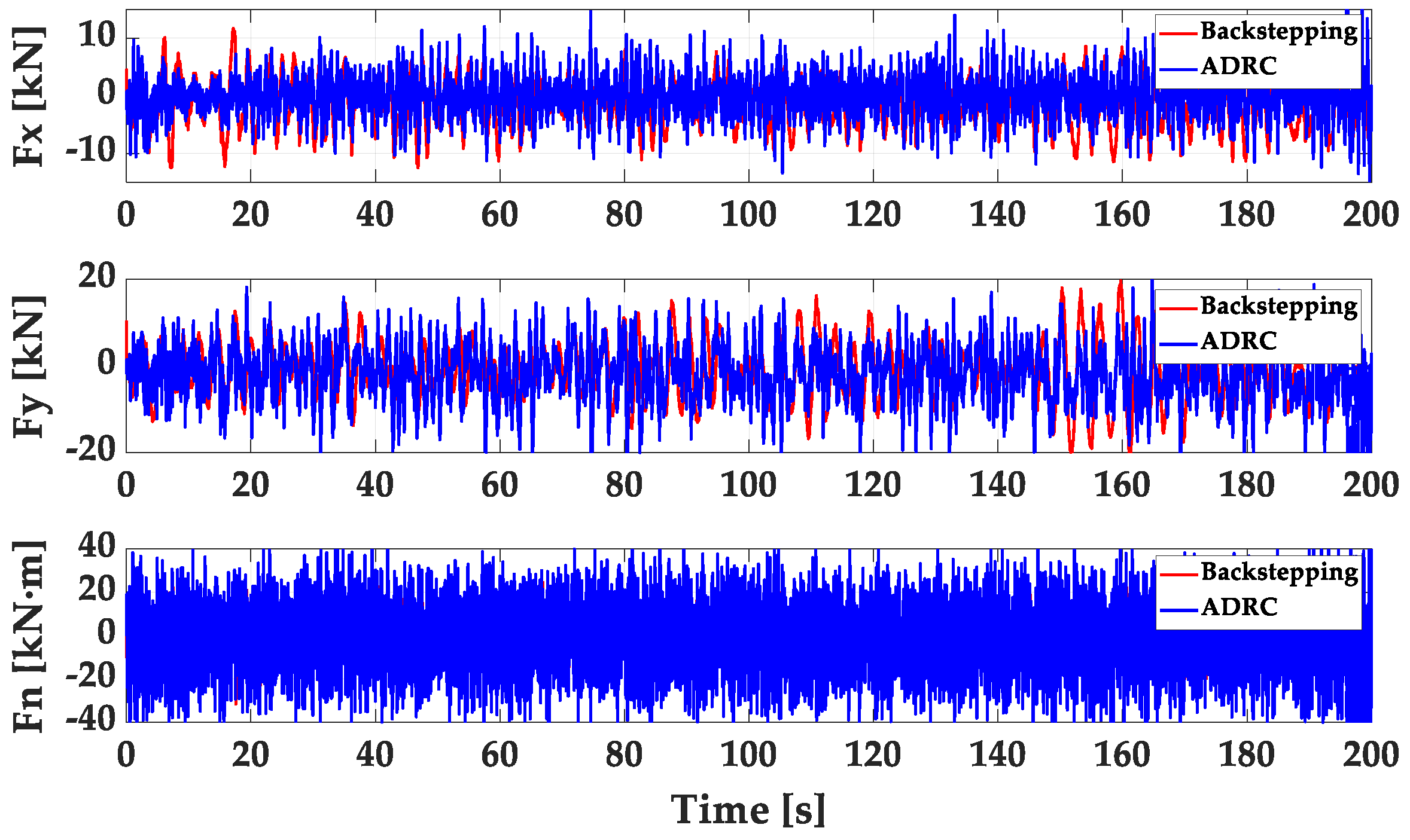
6.1.2. Simulation under Environmental Disturbances

For control system design, it is common to assume the principle of superposition when considering wind and wave disturbances. For most marine control applications, this is a good approximation. In this paper, the fourth-level sea state has 2 m wave height and 10 m/s average wind speed [29,53].

The initial signal and desired signal are still the same as the simulation under ideal sea conditions. The surge, sway, yaw and position under environmental disturbances can be seen in Figure 16 and Figure 17, respectively. The speed of the ship is shown in Figure 18. Figure 19 shows the forces and moment of thrusters under environmental disturbances.

It can be seen from Figure 16 to Figure 17 that after adding environmental disturbances, the ship with the two controllers can still reach the desired position in a state of oscillation due to the influence of wind and wave interference. However, it can be observed that ADRC reveals more stable performance with a smoother trajectory than backstepping and the ADRC is still about 20 s faster than backstepping control to reach the set position. Figure 18 indicates the comparison of the speed of three DOF with ADRC and backstepping control. As can be seen from Figure 18, the speed change trend of ADRC is basically the same as that without disturbances, which oscillates much more slightly than backstepping. It is obvious from Figure 19 that there is a huge fluctuation in the forces and moment of thrusters with disturbances. The maximum abrupt values of forces and moment in the three directions are 10 kN, 20 kN and 40 kN·m, respectively. From the positioning results, it proves that the designed controllers can still realize the positioning function to reach the desired position without large overshooting. ADRC has a stronger anti-interference ability than backstepping control, but the forces and moment both have a fluctuation, which may be harmful to the use of thrusters.

In summary, the use of the classical ADRC can realize the fixed-point positioning control and yaw control of the ship, which proves that ADRC does make the ship reach the desired reference quickly without overshooting and have higher positioning accuracy than backstepping control. However, from the results of forces and moment, there is much room for improvement in the future research.

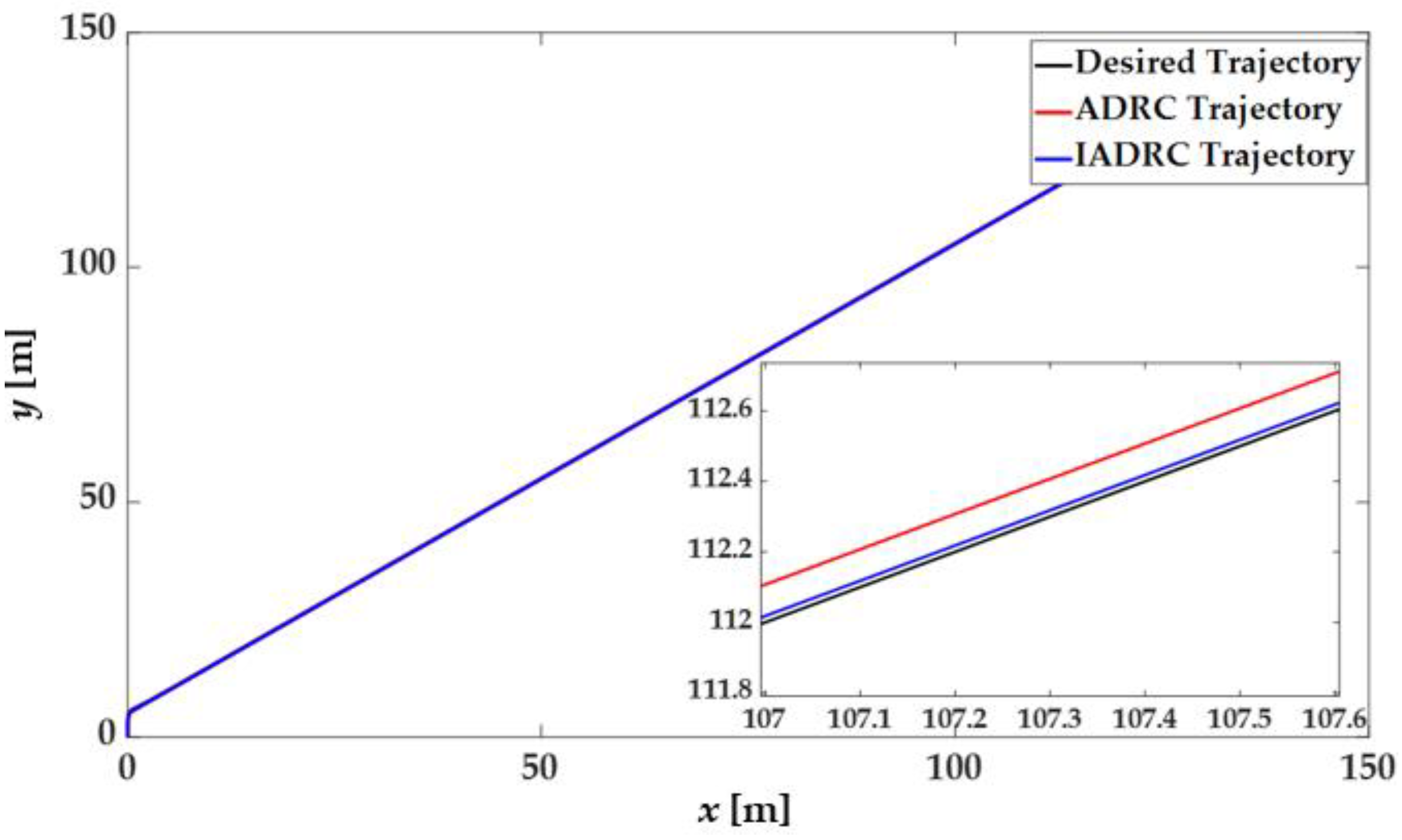
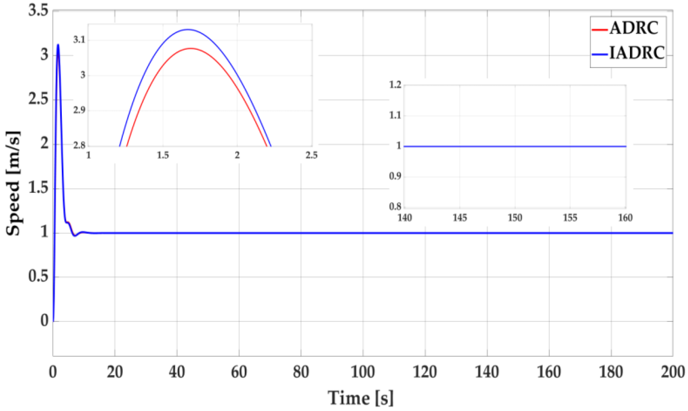
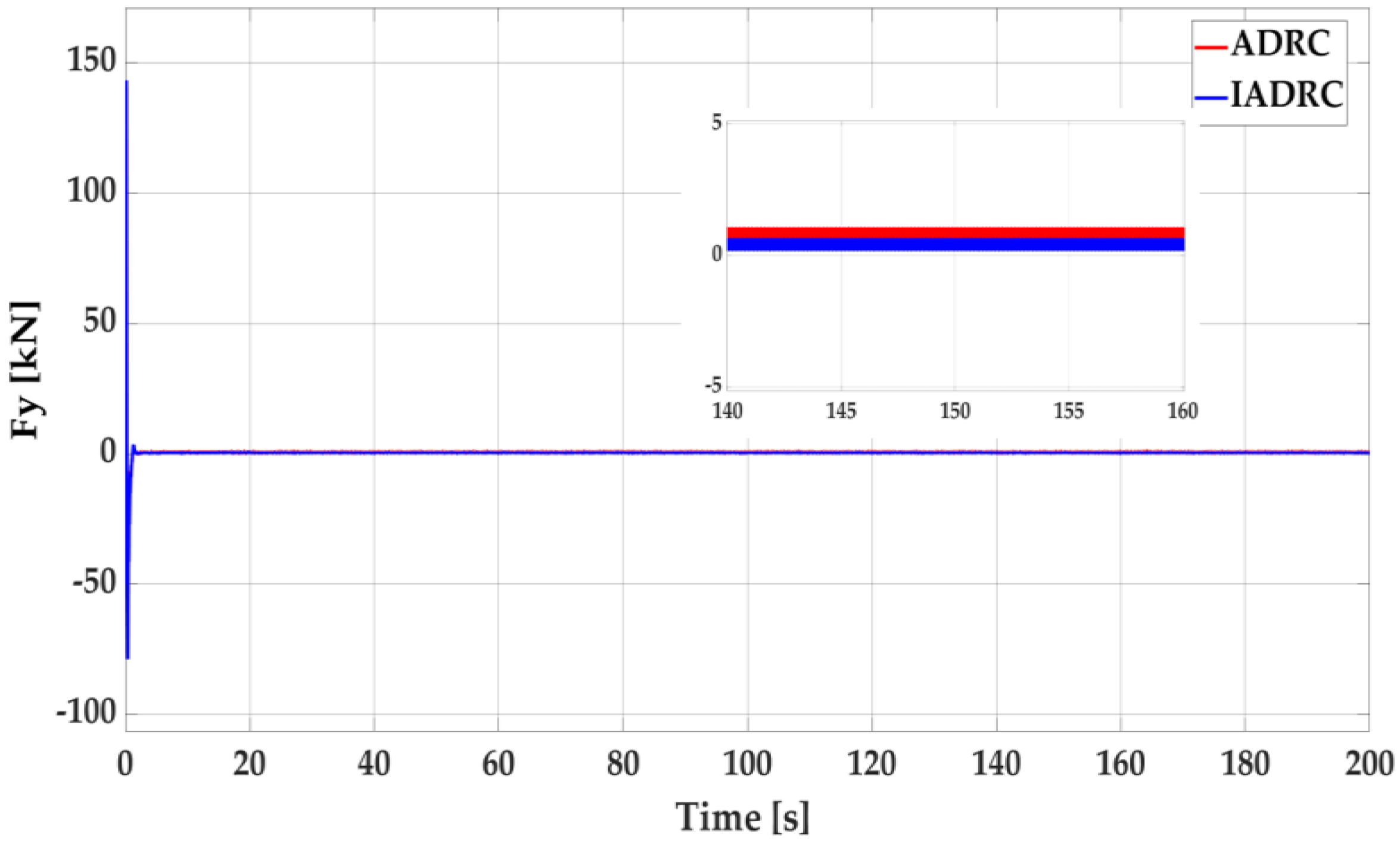
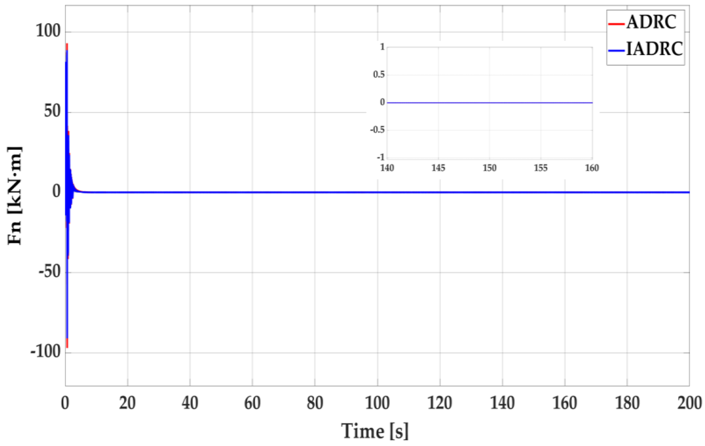
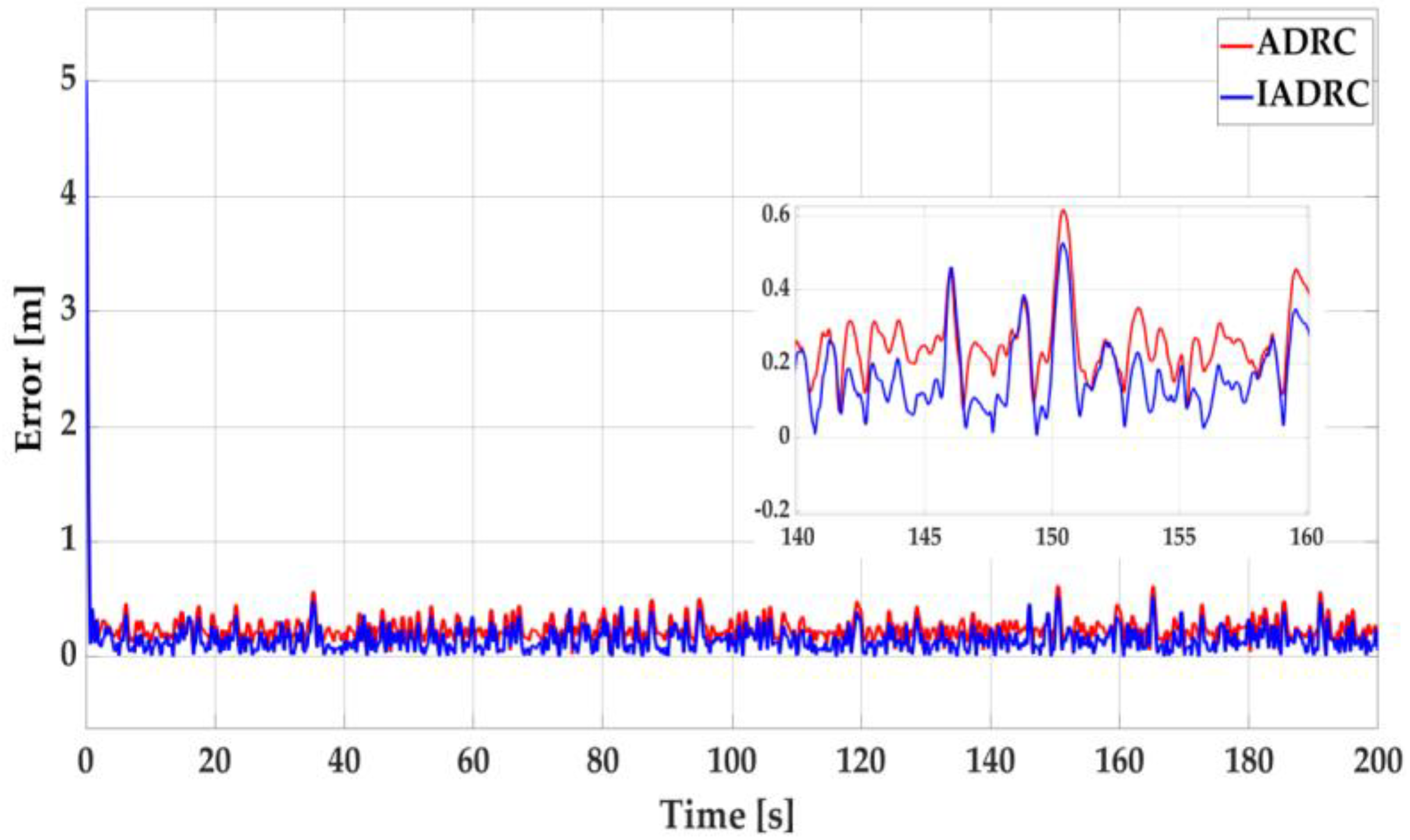
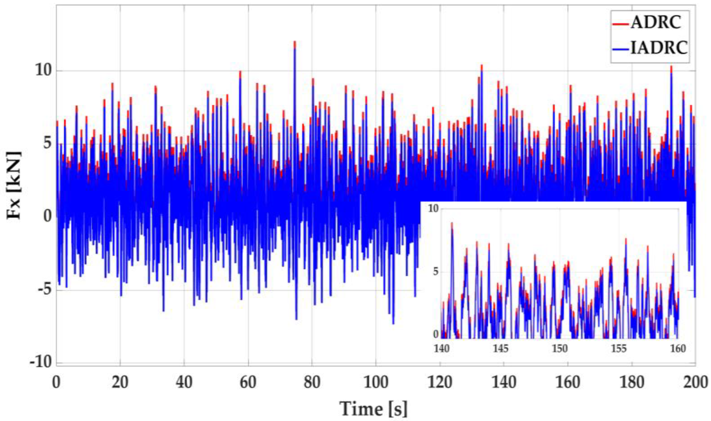
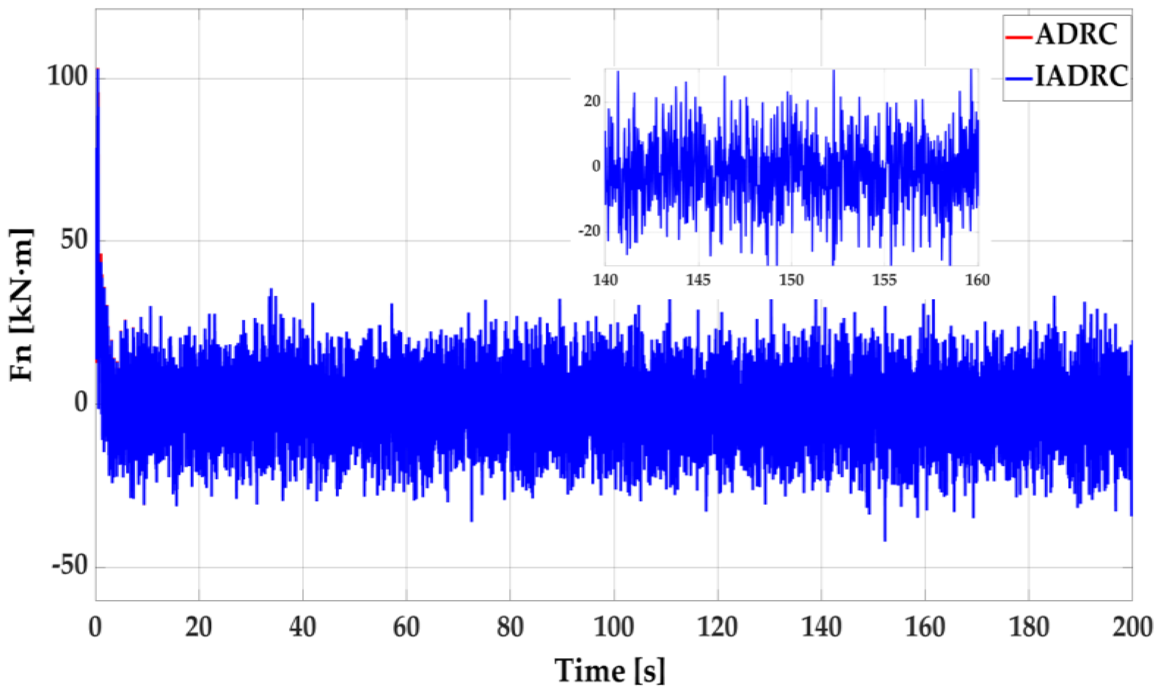
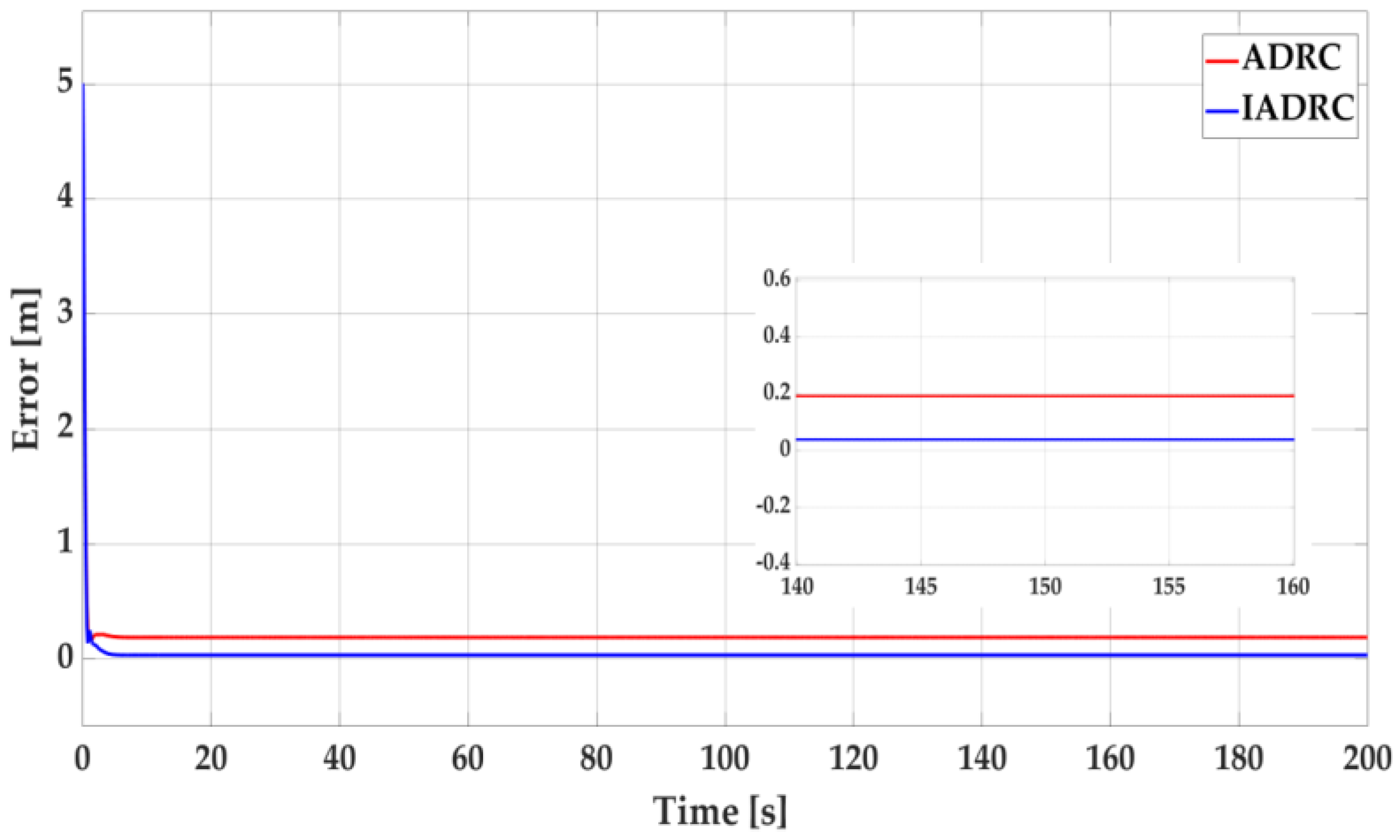
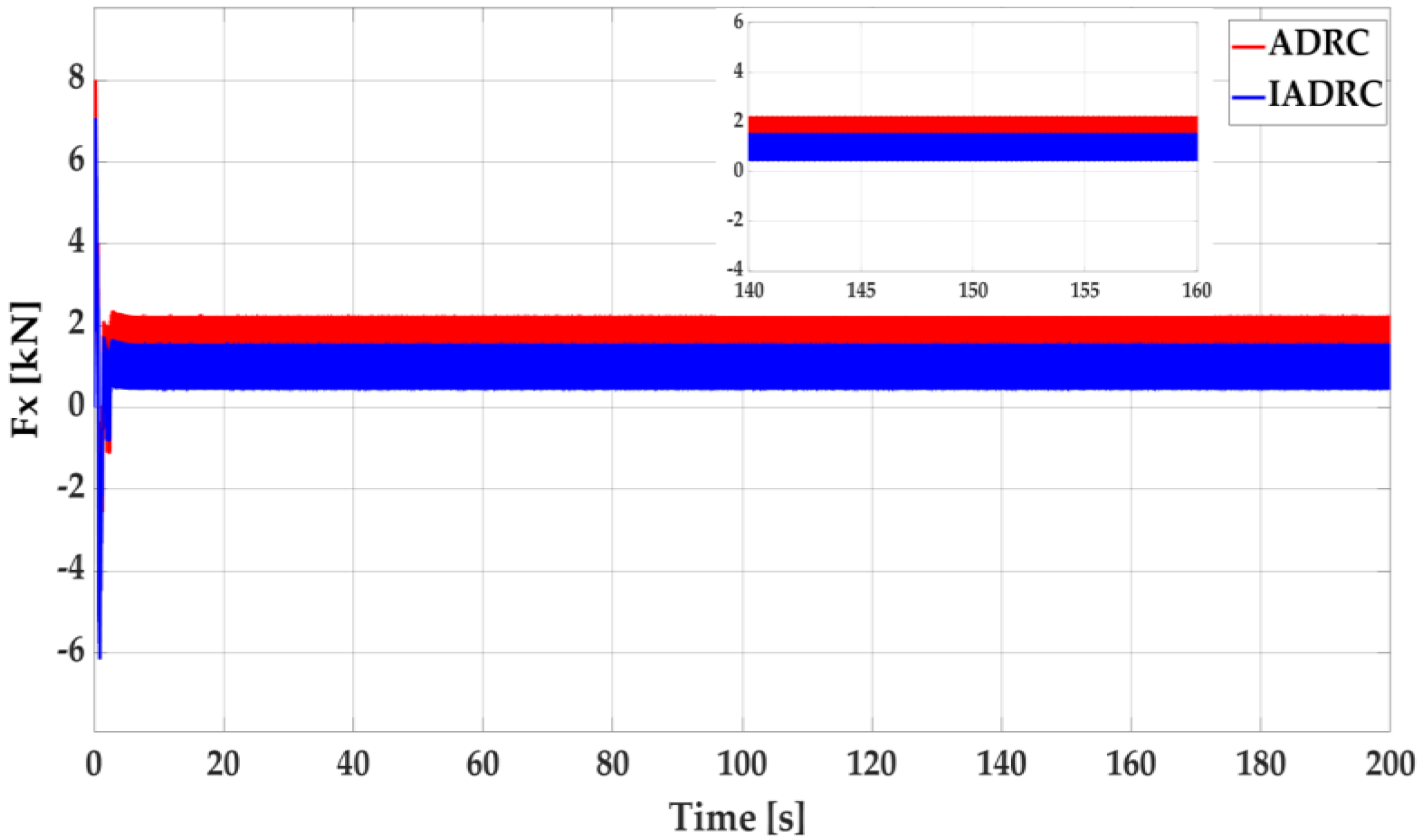
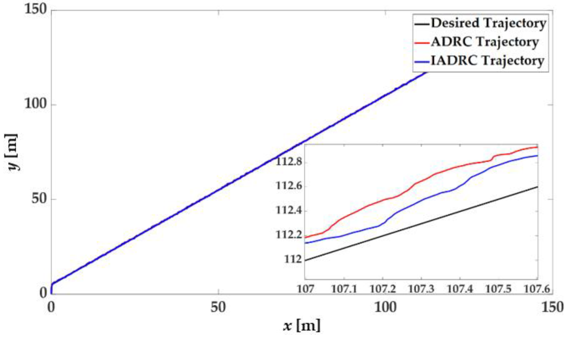
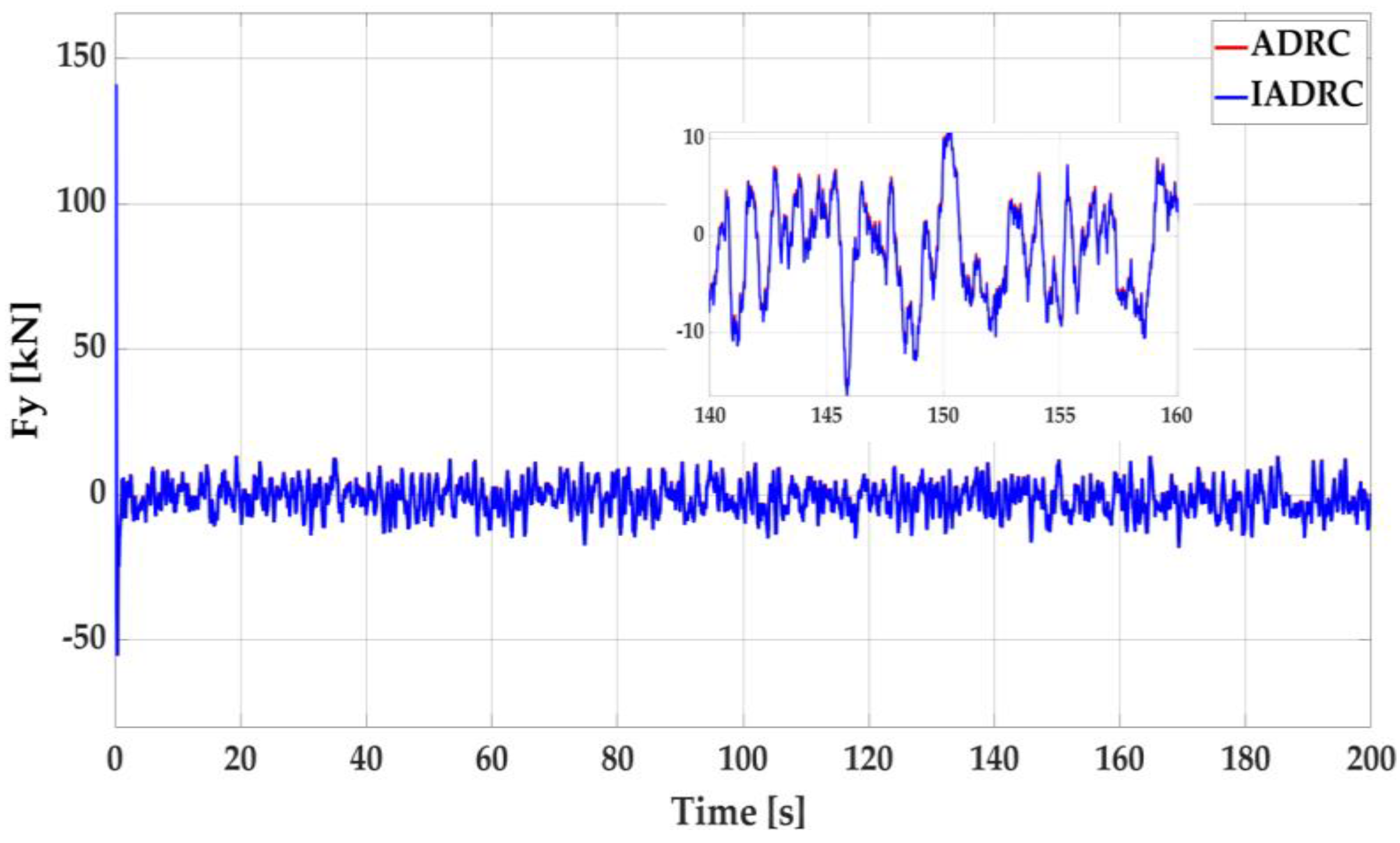
6.2. Straight Track Control Based on IADRC

According to the above simulations and analysis of the fixed-point control and yaw control, the classical ADRC has a better effect than backstepping control. However, according to the analysis in Section 5.1, due to the complexity of track control, the problems of dither and phase delay in the classical ADRC may have an impact on the straight track control, and the classical ADRC may be not suitable in this case. Therefore, the IADRC which has been presented in Section 5.2 is applied and compared with the classic ADRC.

To compare the errors before and after improvement more intuitively, the mean value of the square value of the tracking error is used to compare the size of the tracking error, as shown in Equation (50):

$$\mathsf{\epsilon }=\frac{{\displaystyle \sum }{\mathrm{error}}^2}{\mathrm{n}}$$

(50)

where $\mathrm{error}$ is the distance between the desired position and the actual position and $\mathrm{n}$ is the number of samples. $\mathsf{\epsilon }$ represents the degree to which the actual value deviates from the set value, which is similar to Mean Square Error (MSE) in statistics. MSE is the averaged squared difference between the outputs and the targets [54]. The smaller the MSE is, the less the actual value deviates from the set value and the more stable the system is.

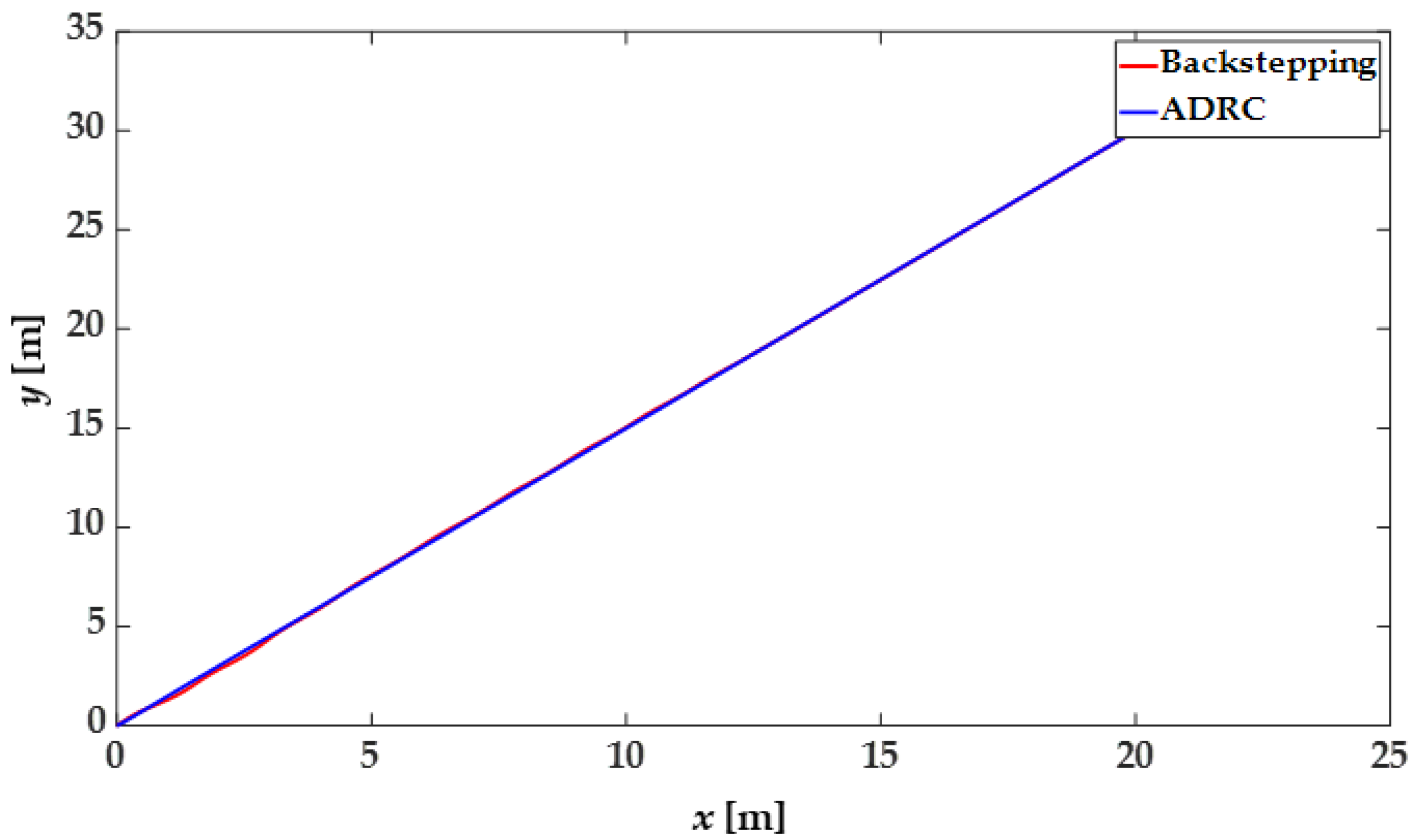
6.2.1. Simulation under Ideal Sea Condition

The initial state of the ship is that the initial position is at the origin of the coordinates. The straight reference track is set as $\mathrm{y}=\mathrm{x}+5$. The set yaw angle is 45° and the set speed is 1 m/s. In the case of low speed, the ship needs to keep the set yaw angle unchanged when sailing along the set trajectory.

First, the environment is ideal sea condition. The simulation time is 200 s. Figure 20 shows the straight track of the ship. Figure 21 shows the tracking error and Figure 22 shows the speed of the ship. Figure 23, Figure 24 and Figure 25 show the forces and moment.

It can be seen from Figure 20 and Figure 21 that both ADRC and IADRC can effectively make the ship track the given trajectory. As is clearly shown in the two figures, the tracking error of the two controllers gradually decreases from 5 m and the tracking error of them is less than 1 m after the ship sails steadily. However, the tracking error of IADRC is smaller than that of classical ADRC, which proves that the DP performance of IADRC is better than that of ADRC under ideal sea condition. According to Equation (50), the error dispersion before and after improvement can be calculated as ${\mathsf{\epsilon }}_1=0.1644$ and ${\mathsf{\epsilon }}_2=0.1260$, respectively, in which ${\mathsf{\epsilon }}_2$ is about 23.4% less than ${\mathsf{\epsilon }}_1$. It indicates that the improved controller brings the trajectory closer to the given track. Figure 22 shows the speed of the ship with the two controllers. It can be seen that the ship starts from the origin, accelerates with a certain acceleration, decelerates after basically synchronizing with the given track, and finally maintains a low speed of about 1 m/s. The maximum speed of the two controllers is around 3.1 m/s. Figure 23, Figure 24 and Figure 25 show the comparison of the forces and moment of three DOF with ADRC and IADRC. In the initial stage of the tracking process, in order to enable the ship to achieve fast tracking, the control forces and moment of thrusters change more rapidly, and the maximum abrupt values of forces and moment in the three directions are 8 kN, 150 kN and 100 kN·m, respectively. Although the forces in surge and sway direction after improvement is smaller than that before improvement, both of the two have severe fluctuation. This analysis shows that the IADRC can reduce the error of straight track control compared with the classical ADRC so that the actual trajectory of the ship is more synchronized with the set trajectory, which ensures the stability of sailing.

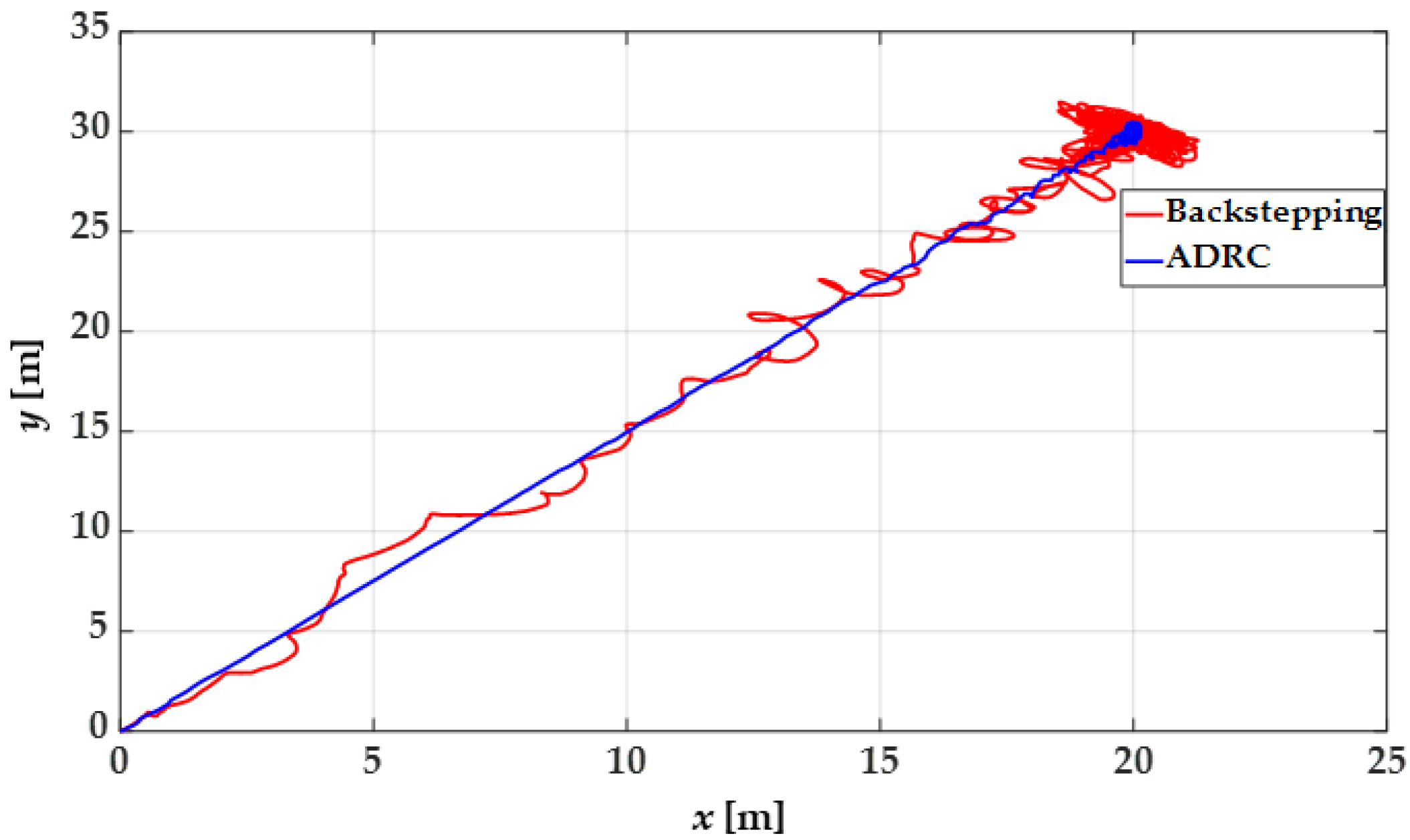
6.2.2. Simulation under Environmental Disturbances

This case considers the straight track control of the ship under the environmental disturbances the same as in the previous case (fixed-point control) and the initial state is the same as Section 6.2.1. Figure 26 shows the straight track of the ship. Figure 27 shows the tracking error and Figure 28 shows the speed of the ship. Figure 29, Figure 30 and Figure 31 show the forces and moment.

It can be seen from Figure 26 to Figure 27 that the two controllers can still realize the straight track control of the ship under the environmental disturbances. According to Equation (50), the error dispersion before and after improvement can be calculated as ${\mathsf{\epsilon }}_1=0.1095$ and ${\mathsf{\epsilon }}_2=0.0736$, respectively, in which ${\mathsf{\epsilon }}_2$ is about 32.8% less than ${\mathsf{\epsilon }}_1$. It indicates that the improved controller brings the track closer to the given track and the error is smaller under the environmental disturbances. The speed of the ship can be stabilized at about 1 m/s and the maximum speed is slightly larger than that under ideal sea condition due to the environmental disturbances. It can be seen in Figure 29, Figure 30 and Figure 31 that the forces and moment of thrusters in the three directions with ADRC or IADRC all have different degrees of oscillation due to external disturbances. The maximum fluctuation amplitude in the surge and sway directions does not exceed about 10 kN and that in the yaw direction is not more than about 20 kN·m. In conclusion, the IADRC can better realize the straight track control of the ship under environmental disturbances according to the positioning results.

From the above analysis, it can be seen that ADRC can achieve fast and accurate tracking both for the fixed-point control and the straight track control, and the IADRC can significantly reduce the error, indicating that the control methods used in this paper have good dynamic control performance. Although the above controllers can all have good results from a position perspective, the results of forces and moment are not perfect, which are also the focuses of future work.

7. Conclusions

This paper focuses on DP control of ships based on ADRC. This paper proposes a new ADRC controller which is significantly improved by the uses of fal function filter and phase prediction. The designed ADRC can realize the fixed-point and yaw control in a short time of about 30 s compared with backstepping control. It can reach the set value without overshoot, and it also has better positioning performance under environmental disturbances. With the fal function filter and phase prediction, the phase delay and dither problems of the tracking differentiator are improved. Compared with the classical ADRC, the IADRC can not only realize the straight track control of the ship, but also effectively reduce the error, among which the degree of the error $\mathsf{\epsilon }$ decreases by 23.4% under ideal sea condition and by 32.8% under external environmental disturbances. The simulations indicate that the proposed methods can meet the requirements of DP and have better positioning performance than more classical methods. However, although the proposed methods can achieve dynamic positioning, they still have some limitations. The forces and moment oscillations are large, which are harmful to the stable operation of the thrusters and may damage the equipment for a long time. Besides, ADRC has many parameters that need to be tuned. Hence, the future work will focus on improving control output and parameter optimization. Artificial intelligence algorithms, conjugate gradient algorithm, sliding mode control or fuzzy control will be considered to optimize control parameters and adjust control output to improve the control effect.

References

1. Wang, S.; Yang, X.; Wang, Z.; Guo, L. Summary of Research on Related Technologies of Ship Dynamic Positioning System. E3S Web. Conf. 2021, 233, 04032. [Google Scholar] [CrossRef]
2. Veksler, A.; Johansen, T.A.; Borrelli, F.; Realfsen, B. Dynamic Positioning with Model Predictive Control. IEEE Trans. Control Syst. Technol. 2016, 24, 1340–1353. [Google Scholar] [CrossRef] [Green Version]
3. Hu, K.; Ding, Y.; Wang, H.; Xiong, D. Analysis of Capability Requirement of Dynamic Positioning System for Cargo Transfer Vessel at Sea. J. Mar. Sci. Appl. 2019, 18, 205–212. [Google Scholar] [CrossRef]
4. Fossen, T.I. A survey on Nonlinear Ship Control: From Theory to Practice. IFAC Proc. Vol. 2000, 33, 1–16. [Google Scholar] [CrossRef]
5. Yuh, J. Design and Control of Autonomous Underwater Robots: A survey. Auton. Robot. 2000, 8, 7–24. [Google Scholar] [CrossRef]
6. Smallwood, D.A.; Whitcomb, L.L. Model-based dynamic positioning of underwater robotic vehicles: Theory and experiment. IEEE J. Ocean. Eng. 2004, 29, 169–186. [Google Scholar] [CrossRef]
7. Sørensen, A.J. A survey of dynamic positioning control systems. Annu. Rev. Control 2011, 35, 123–136. [Google Scholar] [CrossRef]
8. Mehrzadi, M.; Terriche, Y.; Su, C.; Bin, M.; Guerrero, J.M. Review of Dynamic Positioning Control in Maritime Microgrid Systems. Energies 2020, 13, 3188. [Google Scholar] [CrossRef]
9. Xu, S.; Wang, X.; Yang, J.; Wang, L. A fuzzy rule-based PID controller for dynamic positioning of vessels in variable environmental disturbances. J. Mar. Sci. Technol. 2020, 25, 914–924. [Google Scholar] [CrossRef]
10. Zhang, D.; Ashraf, M.A.; Liu, Z.; Peng, W.X.; Mosavi, A. Dynamic modeling and adaptive controlling in GPS-intelligent buoy (GIB) systems based on neural-fuzzy networks. Ad Hoc Netw. 2020, 103, 102149. [Google Scholar] [CrossRef] [Green Version]
11. Øvereng, S.S.; Nguyen, D.T.; Hamre, G. Dynamic Positioning using Deep Reinforcement Learning. Ocean Eng. 2021, 235, 109433. [Google Scholar] [CrossRef]
12. Ryalat, M.; Damiri, H.S.; EIMoaqet, H. Particle Swarm Optimization of a Passivity-Based Controller for Dynamic Positioning of Ships. Appl. Sci. 2020, 10, 7314. [Google Scholar] [CrossRef]
13. Zhang, H.; Wei, X.; Wei, Y.; Hu, X. Anti-disturbance control for dynamic positioning system of ships with disturbances. Appl. Math. Comput. 2021, 396, 125929. [Google Scholar] [CrossRef]
14. Xia, G.; Liu, C.; Zhao, B.; Chen, X.; Shao, X. Finite Time Output Feedback Control for Ship Dynamic Positioning Assisted Mooring Positioning System with Disturbances. Int. J. Control Autom. Syst. 2019, 17, 2948–2960. [Google Scholar] [CrossRef]
15. Li, W.; Sun, Y.; Chen, H.; Wang, G. Model predictive controller design for ship dynamic positioning system based on state-space equations. J. Mar. Sci. Technol. 2017, 22, 426–431. [Google Scholar] [CrossRef]
16. Zheng, H.; Negenborn, R.R.; Lodewijks, G. Trajectory tracking of autonomous vessels using model predictive control. IFAC Proc. Vol. 2014, 47, 8812–8818. [Google Scholar] [CrossRef] [Green Version]
17. Tiwari, K.; Krishnankutty, P. Comparison of PID and LQR Controllers for Dynamic Positioning of an Oceanographic Research Vessel. In Proceedings of the Fifth International Conference in Ocean Engineering (ICOE2019); Sundar, V., Sannasiraj, S.A., Eds.; Springer: Singapore, 2021; Volume 106, pp. 343–354. [Google Scholar]
18. Ashrafiuon, H.; Muske, K.R.; Mcninch, L.C.; Soltan, R.A. Sliding-mode tracking control of surface vessels. IEEE Trans.Ind. Electron. 2008, 55, 4004–4012. [Google Scholar] [CrossRef]
19. Ashrafiuon, H.; Muske, K.R. Sliding mode tracking control of surface vessels. In Proceedings of the 2008 American Control Conference, Washington, DC, USA, 11–13 June 2008. [Google Scholar]
20. Tannuri, E.A.; Agostinho, A.C.; Morishita, H.M.; Moratelli, L. Dynamic positionning systems: An experimental analysis of sliding mode control. Control Eng. Pract. 2010, 18, 1121–1132. [Google Scholar] [CrossRef]
21. Alattas, K.A.; Mobayen, S.; Din, S.U.; Asad, J.H.; Fekih, A.; Assawinchaichote, W.; Vu, A.M.T. Design of a Non-Singular Adaptive Integral-Type Finite Time Tracking Control for Nonlinear Systems with External Disturbances. IEEE Access 2021, 9, 102091–102103. [Google Scholar] [CrossRef]
22. Vu, M.T.; Thanh, H.L.N.N.; Huynh, T.T.; Do, Q.T.; Do, T.D.; Hoang, Q.D.; Le, T.H. Station-keeping control of a hovering over-actuated autonomous underwater vehicle under ocean current effects and model uncertainties in the horizontal plane. IEEE Access 2021, 9, 6855–6867. [Google Scholar] [CrossRef]
23. Vu, M.T.; Le, T.H.; Thanh, H.L.N.N.; Huynh, T.T.; Van, M.; Hoang, Q.D.; Do, T.D. Robust Position Control of an Over-actuated Underwater Vehicle under Model Uncertainties and Ocean Current Effects Using Dynamic Sliding Mode Surface and Optimal Allocation Control. Sensors 2021, 21, 747. [Google Scholar] [CrossRef] [PubMed]
24. Piao, Z.; Guo, C.; Sun, S. Adaptive Backstepping Sliding Mode Dynamic Positioning System for Pod Driven Unmanned Surface Vessel Based on Cerebellar Model Articulation Controller. IEEE Access 2020, 8, 48314–48324. [Google Scholar] [CrossRef]
25. Hu, Y.; Park, G.K.; Wu, H.; Zhang, Q. Robust Adaptive Fuzzy Design for Ship Linear-tracking Control with Input Saturation. Int. J. E-Navi. Marit. Econ. 2017, 6, 9–16. [Google Scholar] [CrossRef]
26. Zhao, J.; Du, J.; Yu, S.; Liu, Y. Adaptive nonlinear controller design for course-tracking of ships based on dynamic surface control and backstepping. In Proceedings of the 31st Chinese Control Conference, Hefei, China, 25–27 July 2012. [Google Scholar]
27. Li, J.; Xiang, X.; Yang, S. Robust adaptive neural network control for dynamic positioning of marine vessels with prescribed performance under model uncertainties and input saturation. Neurocomputing 2022, 484, 1–12. [Google Scholar] [CrossRef]
28. Du, J.; Hu, X.; Liu, H.; Chen, C.L. Adaptive Robust Output Feedback Control for a Marine Dynamic Positioning System Based on a High-Gain Observer. IEEE Trans. Neural Netw. Learn. Syst. 2015, 26, 2775–2786. [Google Scholar] [CrossRef]
29. Fossen, T.I. Marine Control Systems: Guidance, Navigation and Control of Ships, Rigs and Underwater Vehicles; Marine Cybernetics AS: Trondheim, Norway, 2002. [Google Scholar]
30. Du, J.; Yang, Y.; Wang, D.; Guo, C. A robust adaptive neural networks controller for maritime dynamic positioning system. Neurocomputing 2013, 110, 128–136. [Google Scholar] [CrossRef]
31. Hu, X.; Du, J.; Shi, J. Adaptive fuzzy controller design for dynamic positioning system of vessels. Appl. Ocean Res. 2015, 53, 46–53. [Google Scholar] [CrossRef]
32. Peng, X.; Zhang, B.; Rong, L. A robust unscented Kalman filter and its application in estimating dynamic positioning ship motion states. J. Mar. Sci. Technol. 2019, 24, 1265–1279. [Google Scholar] [CrossRef]
33. Ngongi, W.E.; Du, J.; Wang, R. Design of generalised predictive controller for dynamic positioning system of surface ships. Int. Syst. Technol. Appl. 2020, 19, 17–35. [Google Scholar]
34. Gao, Q.; Song, L.; Yao, J. RANS Prediction of Wave-Induced Ship Motions, and Steady Wave Forces and Moments in Regular Waves. J. Mar. Sci. Eng. 2021, 9, 1459. [Google Scholar] [CrossRef]
35. Borkowski, P. Numerical Modeling of Wave Disturbances in the Process of Ship Movement Control. Algorithms 2018, 11, 130. [Google Scholar] [CrossRef] [Green Version]
36. Isherwood, R.M. Wind resistance of merchant ships. Int. J. Marit. Eng. 1972, 114, 327–338. [Google Scholar]
37. Wang, B.; Yang, J.; Jiao, H.; Zhu, K.; Chen, Y. Design of auto disturbance rejection controller for train traction control system based on artificial bee colony algorithm. Measurement 2020, 160, 107812. [Google Scholar] [CrossRef]
38. Han, J. Active Disturbance Rejection Control Technique-the Technique for Estimating and Compensating the Uncertainties, 1st ed.; National Defense Industry Press: Beijing, China, 2008; pp. 97–107. (In Chinese) [Google Scholar]
39. Han, J. From PID to Active Disturbance Rejectio Control. IEEE Trans. Ind. Electron. 2009, 56, 900–906. [Google Scholar] [CrossRef]
40. Xie, H. Absolute Stability Theory and Application; Science Press: Beijing, China, 1986. (In Chinese) [Google Scholar]
41. Ye, Y.; Bai, M.; Zhang, Z.; Qiu, W.; Rui, L. A design of dredger cutter motor synchronous speed control system based on ADRC. In Proceedings of the 28th Chinese Control and Decision Conference (CCDC), Yinchuan, China, 28–30 May 2016. [Google Scholar]
42. Hu, J.; Ge, Y.; Zhou, X.; Liu, S.; Wu, J. Research on the course control of USV based on improved ADRC. Syst. Sci. Control Eng. 2020, 9, 44–51. [Google Scholar] [CrossRef]
43. Wu, Z.; Gao, Z.; Li, D.; Chen, Y.; Liu, Y. On transitioning from PID to ADRC in thermal power plants. Control Theory Technol. 2021, 19, 3–18. [Google Scholar] [CrossRef]
44. Wang, Y.; Yang, Y.; Ding, F. Improved ADRC control strategy in FPSO dynamic positioning control application. In Proceedings of the 2016 IEEE International Conference on Mechatronics and Automation, Harbin, China, 7–10 August 2016. [Google Scholar]
45. Lei, Z.; Guo, C. Noise suppression by ADRC for ship positioning and yaw control. In Proceedings of the 32nd Chinese Control Conference (CCC), Xi’an, China, 26–28 July 2013. [Google Scholar]
46. Dong, Z.; Zhang, J. An active disturbance rejection controller design for ball and plate system. In Proceedings of the 34th Chinese Control Conference (CCC), Hangzhou, China, 28–30 July 2015. [Google Scholar]
47. Ye, B.; Xiong, J.; Wang, Q.; Luo, Y. Design and Implementation of Pseudo-Inverse Thrust Allocation Algorithm for Ship Dynamic Positioning. IEEE Access 2020, 8, 16830–16837. [Google Scholar] [CrossRef]
48. Wang, B. ROV Dynamic Positioning. In Encyclopedia of Ocean Engineering; Cui, W., Fu, S., Hu, Z., Eds.; Springer: Singapore, 2020; pp. 1–8. [Google Scholar]
49. Zheng, Q.; Chen, Z.; Gao, Z. A practical approach to disturbance decoupling control. Control Eng. Pract. 2009, 17, 1016–1025. [Google Scholar] [CrossRef] [Green Version]
50. Zhang, C.; Wang, X.; Xiao, J. Ship dynamic positioning system based on backstepping control. J. Theor. Appl. Inf. Technol. 2013, 51, 129–136. [Google Scholar]
51. Jin, Z.; Zhang, W.; Liu, S.; Gu, M. Command-Filtered Backstepping Integral Sliding Mode Control with Prescribed Performance for Ship Roll Stabilization. Appl. Sci. 2019, 9, 4288. [Google Scholar] [CrossRef] [Green Version]
52. Song, Y.; Xu, R.; Wang, Q.; Song, Z.; Zhao, B.; Zhang, M. Study on Ship Dynamic Positioning with Stochastic Backstepping Nonlinear Controller. In Proceedings of the 2019 Chinese Control and Decision Conference (CCDC), Nanchang, China, 3–5 June 2019. [Google Scholar]
53. Fossen, T.I. Guidance and Control of Ocean Vehicles; John Wiley and Sons: Chichester, UK, 1994; pp. 57–67. [Google Scholar]
54. Ahmed, S.; Sultana, Q.; Deergha Rao, K. Comparative analysis of DGPS predicted corrections using dynamic neural networks. In Proceedings of the 2014 IEEE International Conference on Vehicular Electronics and Safety, Hyderabad, India, 16–17 December 2014. [Google Scholar]
Figure 1. A cable laying vessel with DP system [3].
Jmse 10 00865 g001
Figure 2. (a) The NED coordinate and (b) Body-fixed coordinate [28].
Jmse 10 00865 g002
Figure 3. The structure of ADRC [42].
Jmse 10 00865 g003
Figure 4. Single control of TD.
Jmse 10 00865 g004
Figure 5. The output of TD.
Jmse 10 00865 g005
Figure 6. The feedback structure of fal function filter [45].
Jmse 10 00865 g006
Figure 7. The tracking signal after fal function filter.
Jmse 10 00865 g007
Figure 8. The principle figure of phase prediction.
Jmse 10 00865 g008
Figure 9. The output of IADRC.
Jmse 10 00865 g009
Figure 10. The principle of IADRC.
Jmse 10 00865 g010
Figure 11. The structure of DP system [48].
Jmse 10 00865 g011
Figure 12. The position of surge, sway and yaw under ideal sea condition.
Jmse 10 00865 g012
Figure 13. The trajectory of the ship under ideal sea condition.
Jmse 10 00865 g013
Figure 14. The speed of the ship under ideal sea condition.
Jmse 10 00865 g014
Figure 15. The forces and moment under ideal sea condition.
Jmse 10 00865 g015
Figure 16. The position of surge, sway and yaw under environmental disturbances.
Jmse 10 00865 g016
Figure 17. The trajectory of the ship under environmental disturbances.
Jmse 10 00865 g017
Figure 18. The speed of the ship under environmental disturbances.
Jmse 10 00865 g018
Figure 19. The forces and moment under environmental disturbances.
Jmse 10 00865 g019
Figure 20. The straight track of the ship under ideal sea condition.
Jmse 10 00865 g020
Figure 21. Tracking error under ideal sea condition.
Jmse 10 00865 g021
Figure 22. The speed of the ship under ideal sea condition.
Jmse 10 00865 g022
Figure 23. The Force in the surge direction under ideal sea condition.
Jmse 10 00865 g023
Figure 24. The Force in the sway direction under ideal sea condition.
Jmse 10 00865 g024
Figure 25. The Moment in the yaw direction under ideal sea condition.
Jmse 10 00865 g025
Figure 26. The straight track of the ship under environmental disturbances.
Jmse 10 00865 g026
Figure 27. Tracking error under environmental disturbances.
Jmse 10 00865 g027
Figure 28. The speed of the ship under environmental disturbances.
Jmse 10 00865 g028
Figure 29. The force in the surge direction under environmental disturbances.
Jmse 10 00865 g029
Figure 30. The force in the sway direction under environmental disturbances.
Jmse 10 00865 g030
Figure 31. The moment in the yaw direction under environmental disturbances.
Jmse 10 00865 g031