Seabed Sediment Classification Using Spatial Statistical Characteristics

Abstract

Conventional sediment classification methods based on Multibeam Echo System (MBES) data have low accuracy since the correlation between features and sediment has not been fully considered. Moreover, their poor resistance to the residual error of MBES backscatter strength (BS) processing also degrades their performances. Toward these problems, we propose a seabed sediment classification method using spatial statistical features extracted from angular response curve (ARC), topography, and geomorphology. First, to reduce interference of noise and residual error of beam pattern correction, we propose a robust method combining the Generic Seafloor Acoustic Backscatter (GSAB) model and Huber loss function to estimate the parameters of ARC which is strongly correlated with seabed sediments. Second, a feature set is constructed by AR features composed of GSAB parameters, BS mosaic and its derivatives, and seabed topography and its derivatives to characterize seabed sediments. After that, feature selection and probability map acquisition are employed based on the random forest algorithm (RF). Finally, a denoising and final sediment map generation method is proposed and applied to probability maps to obtain the sediment map with reasonable sediment distribution and clear boundaries between classes. We implement experiments and achieve the classification accuracy of 93.3%, which verifies the validity of our method.

1. Introduction

The increase in human activities has had a significant impact on the global water system and underwater benthic environments, and the study and protection of these are essential for the sustainable development of mankind [1,2]. As an important part of the underwater environments, the seabed sediment map is the fundamental geographic information of the marine environment, utilization of marine resources, marine fisheries, and marine science. However, the interpretation of types and distribution of seabed sediments was mainly implemented by grab sampling [3], which is time-consuming, laborious, and difficult to obtain accurate boundaries of various sediments because of the low spatial resolution. MBES has the capability of measuring seafloor topography with high precision, high resolution, and full coverage, and the BS of acoustic signal of MBES can characterize different sediments. Therefore, the method using MBES data to map the seabed sediments will greatly make up for the shortcomings of conventional sampling methods [4].

Researchers have conducted a lot of works on the seabed sediment classification based on BS mosaics. Preston J. [5] and Brown C. J. et al. [6] divided the BS mosaic into fixed-size rectangular units and extracted 132 features such as gray-scale statistics, texture, power spectrum, and fractal dimension to classify seabed sediments. Koop L. et al. [7] classified sediments based on bathymetry and its derivatives to prove the validity of terrain features in sediments mapping by comparing with the classification results based on BS mosaic. Classification methods considering topographic or geomorphologic geometric features are hard to achieve high accuracy performance since acoustic response characteristics of sediments are not taken into account. Thus, Xiaodong Shang et al. [8] used an object-based image analysis method to extract the terrain features and BS mosaic features for sediment classification. Xue Ji et al. [9] extracted a total of 40-dimensional features, including BS mosaic texture features and terrain features, and finally selected the 18-dimensional features to classify sediments.

These methods that utilize geometric features, which are related to spatial distribution characteristics of topography and geomorphology, such as slope, etc., do not take into account physical features, which are related to sediment acoustic properties, such as BS, ARC, etc., and the extracted features may have weak correlations with sediments. Thus, these methods may have the inadequate capability to distinguish some types of sediment which have similarities in terms of terrain and BS mosaic.

The angular response expresses the law that BS changes with the incident angle of the acoustic signal at the seafloor. AR is the characteristic of sediment scattered acoustic signal. Clarke et al. [10] used the differential method to extract the relevant parameters from ARC to characterize sediments. The differential method having poor robustness is unable to obtain the parameters of ARC efficiently and is not suitable for the automatic calculation of large datasets. Shaohua Jin et al. [11] comprehensively analyzed AR and probability distribution of BS, portrayed a 3D histogram, and proposed a method of seafloor classification based on the 3D histogram of BS. Fanlin Yang et al. [12] proposed a seafloor classification method based on a convolutional neural network (CNN). The feature vectors, including BS features and terrain features, are converted into waveform maps, and then input to the CNN for training and classification. Rozaimi Che Hasan [13] extracted the four attributes of angular response data such as mean, slope, skewness, and kurtosis from 30° to 50° incident angles as AR features. However, these parameters are susceptible to noise interference, and only reflect the AR characteristics of the partial angles, leading to weak sediment correlation and loss of classification accuracy.

To better describe the characteristics of BS data using ARC, Hellequin [14] constructed an AR model for the entire range of incident angles based on the different acoustic scattering characteristics at different incident angles, namely the GSAB model. The GSAB model can not only fit the BS well but also resist the interference of random errors of measurement. Shaohua Jin et al. [15] used the least squares method to fit GSAB to extract model parameters as AR features and conducted unsupervised classification to map the sediments. However, due to the complexity of the beam pattern and the incomplete correction, the beam pattern residuals are often contained in BS [16], resulting in deviations in the GSAB parameters. Thus, it is the key to effectively utilizing GSAB parameters as AR features and improving classification accuracy to study the robust estimation method of GSAB parameters to improve the reliability of the model parameters.

In addition to the calculation of features, the classification unit is also a key issue. Object-oriented classification methods are complex and time-consuming, while pixel-oriented classification methods are simple and time-saving, but are severely affected by noise [17]. Therefore, we need to find suitable denoising algorithms for pixel-oriented classification methods.

Aiming to solve the problem of low classification accuracy caused by the weak correlation between features and sediments, as well as the weak robustness to the residual error of BS processing using GSAB parameters as AR features, we propose a robust estimation method for AR feature extraction and integrate AR features, terrain features, and BS mosaic features as a feature set. After the RF feature optimization and probability map acquisition using the feature set, a denoising and final sediment map generation method is proposed and the sediment map with reasonable sediments distribution and clear boundaries between classes can be obtained.

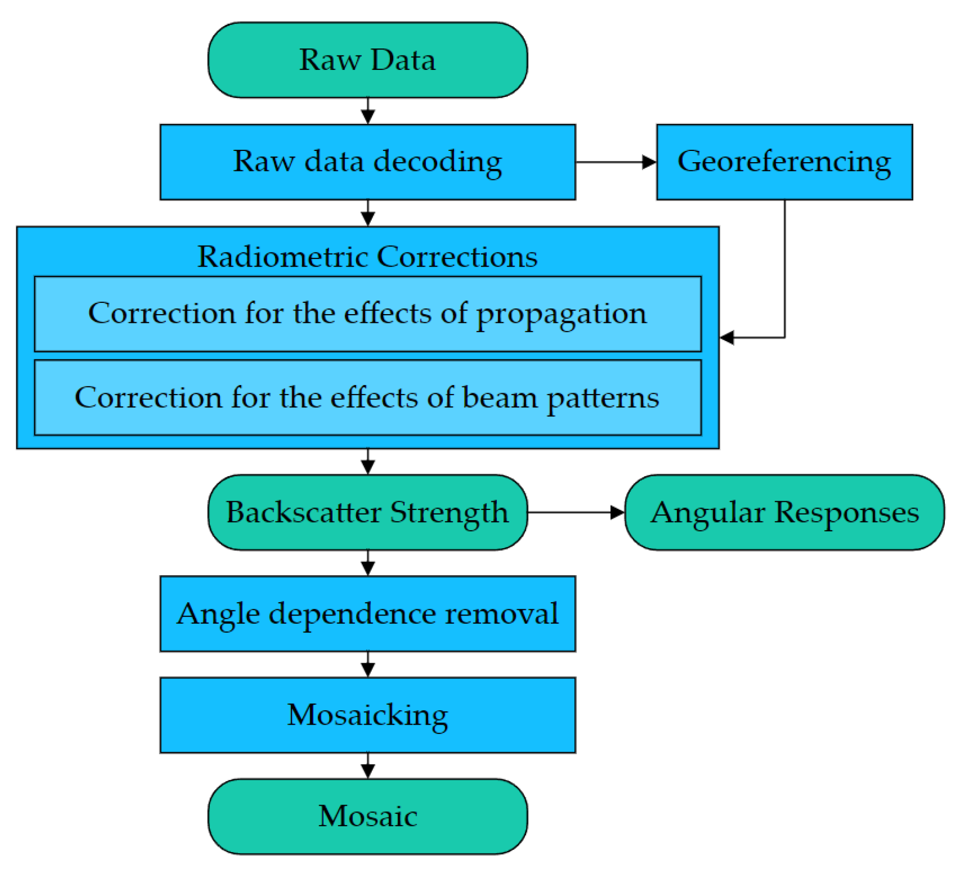
2. Methods

Before the classification, MBES backscatter data are processed through raw data decoding [18], georeferencing [19], Radiometric corrections [20], angle dependence removal [21], and mosaicking [18]. The flowchart of MBES backscatter data processing is shown in Figure 1. Then, the proposed acoustic sediment classification method is applied to obtain the sediment map. The flowchart is shown in Figure 2.

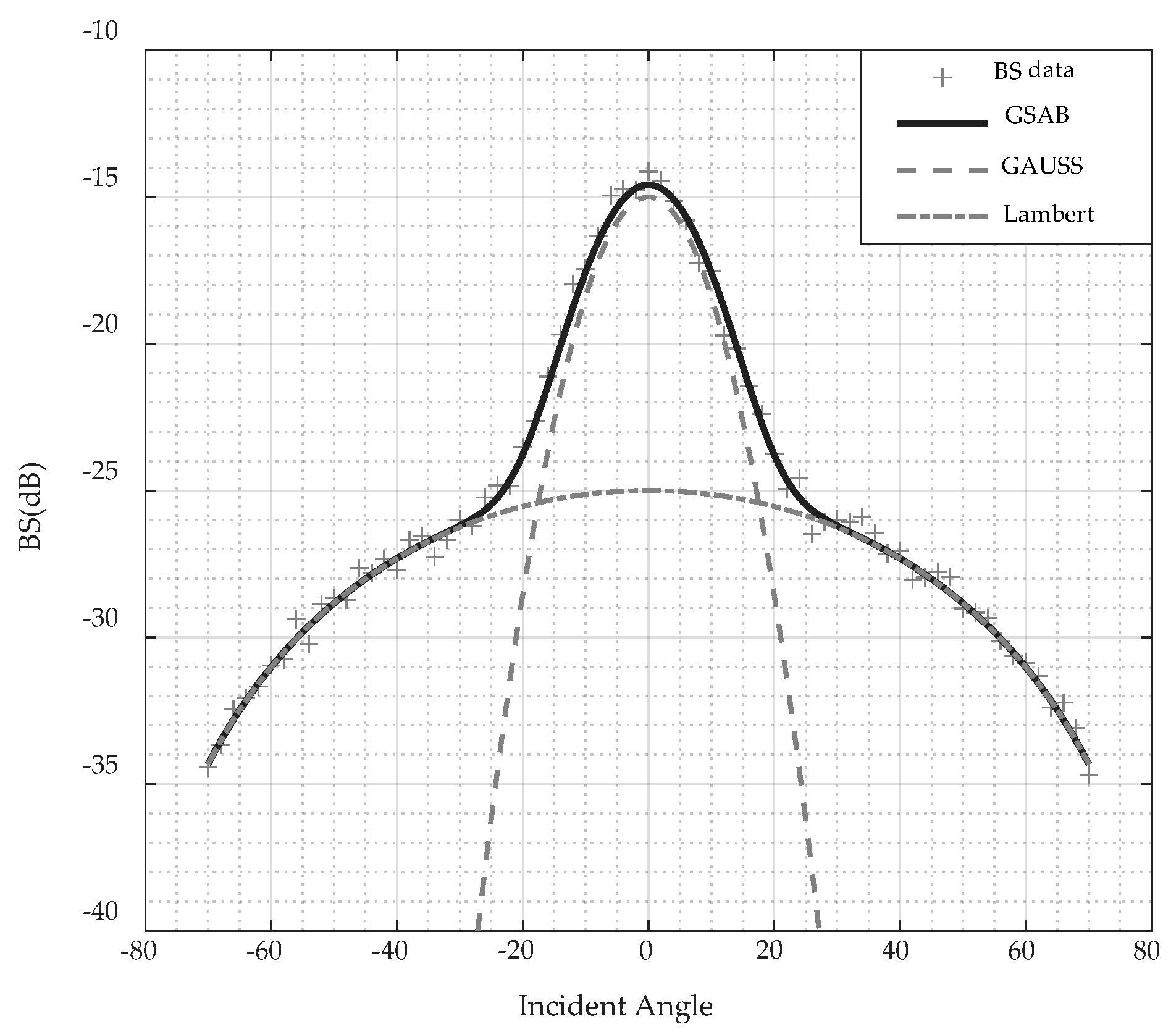
2.1. Robust Estimation of ARC with the GSAB Model and Huber Regression

The ARC, the variation of the BS with incident angle, is strongly correlated with the sediment [22]. The BS contains noise, beam pattern residuals, etc., which deduce the accuracy of AR features. Therefore, a robust estimation method of AR features combined with the GSAB model and Huber regression is proposed to resist the interference of outliers and noise.

The BS achieves its maximum at the vertical incident angle of the beam and decreases with increasing incident angle. The GSAB model uses Lambert’s Law to describe the variation of the BS at obliquely incident angles and uses a Gaussian function to fit the variation of the BS near the vertical incident angles [22] (as shown in Figure 3). The GSAB model is as follows:

$$BS\left(\theta \right)=10\log \left[A\exp \left(-{\theta }^2/2B^2\right)+C{\cos }^D\theta \right]$$

(1)

where A quantifies the maximum amplitude of the specular reflection region. A is related to the coherent reflection coefficient of the water-seabed interface, therefore, A is high in smooth seabed surface and water-seabed interface with high impedance contrast [23,24]. B quantifies the angular range of the specular reflection area and indicates half of the actual reflection range. In the tangent plane model, B represents the difference in the slope of the tiny tangent surface of the seafloor, so B is related to the roughness of the water-seabed interface. C quantifies the average level of BS for grazing angles, and its value increases with increasing acoustic frequency, seafloor roughness, and sediment acoustic impedance. D quantifies the decay rate of the BS with the increasing grazing angle. D is high in soft sediment and smooth seafloor.

The angular response curves obtained by the least squares method are biased due to the effects of beam pattern residuals and noise. Therefore, we use the Huber regression to weaken the side effects of outliers on model parameters.

GSAB is a nonlinear model and needs to be linearized to facilitate parameter calculation. According to the Taylor formula, the first-order expansion is as follows:

$$\begin{array}{l}BS\left(\theta \right)=B{S}_0\left(\theta \right)-q_A{A}_0-q_B{B}_0-q_C{C}_0-q_D{D}_0\\ +q_{A}A+q_{B}B+q_{C}C+q_{D}D+r\\ B{S}_0\left(\theta \right)=10{\log }_{10}\left(A_0\exp \left(\frac{-{\theta }^2}{2B_0{}^2}\right)+C_0{\cos }^{D_0}\theta \right)\\ q_A=q_0\exp \left(\frac{-{\theta }^2}{2B_0{}^2}\right)\\ q_B=q_0{A}_0\exp \left(\frac{-{\theta }^2}{2B_0{}^2}\right)·\frac{{\theta }^2}{B_0{}^3}\\ q_C=q_0{\cos }^{D_0}\theta \\ q_D=q_0{C}_0{\cos }^{D_0}\theta ·\ln \left(\cos \theta \right)\\ q_0=\frac{10}{\left(A_0\exp \left(\frac{-{\theta }^2}{2B_0{}^2}\right)+C_0{\cos }^{D_0}\theta \right)\ln 10}\end{array}$$

(2)

where, $A_0$, $B_0$, $C_0$, and $D_0$ are the initial values of A, B, C, and D, respectively.

Thus the following linear model is constituted:

$$\begin{array}{l}Y={\beta }^{T}X\\ Y=BS\left(\theta \right)-B{S}_0\left(\theta \right)+\left[A_0\hspace{1em}{B}_0\hspace{1em}{C}_0\hspace{1em}{D}_0\right]\left[\begin{array}{c}{q}_A\\ q_B\\ q_C\\ q_D\end{array}\right]\\ \beta ={[A\hspace{1em}B\hspace{1em}C\hspace{1em}D\hspace{1em}]}^T\\ X={\left[q_A\hspace{1em}{q}_B\hspace{1em}{q}_C\hspace{1em}{q}_D\right]}^T\end{array}$$

(3)

Huber regression classifies data into two categories based on error and threshold: outliers which are the data with the error values greater than the threshold, and inliers which are the data with error values less than the threshold. The Huber regression method constructs a loss function by calculating the quadratic loss of inliers and the linear loss of outliers to reduce the weight of outliers. The gradient descent method is then employed to optimize the regression model [25]. The loss function to be minimized by Huber regression is formulated as follows:

$$\begin{gathered} \underset{\beta ,\sigma }{\min }{\displaystyle \sum _{i=1}^n{H}_{\epsilon }\left(\frac{y_i-x_i{}^T\beta }{\sigma }\right)} \\ {H}_{\epsilon }\left(z\right)=\{\begin{array}{cc}{z}^2,& \mathrm{if}\hspace{1em}\left|z\right|<\epsilon \\ 2\epsilon \left|z\right|-{\epsilon }^2,& \mathrm{otherwise}\end{array} \end{gathered}$$

(4)

where i = 1, 2, …, n is the sample data. ε is the threshold for classifying outliers. σ is the standard deviation of the residual, to ensure that $y_i-x_i^T\beta$ is scaled according to a certain ratio so that rescaling ε is not required to achieve the same robustness.

2.2. Extraction of Geometric Features

There is a correlation between topographic and geomorphic features and seabed sediments [26]. We extract depth, slope, aspect, and curvature as topographic features, as shown in

Table 1. Topographic and geomorphic features.

Types	Definition	Variable	Formula	Notes
Topography	Bathymetry	z	$f\left(x,y\right)$	x, y are geographical coordinates
	Slope	slope	$\arctan \sqrt{p^2+q^2}$	$p=\partial z/\partial x$$, q=\partial z/\partial y$
	Aspect	aspect	$180°-\arctan \frac{p}{q}+90°\frac{p}{\left|p\right|}$
	Surface curvature	curvature	$-\frac{1+q^{2}r-2pqs+\left(1+p^2\right)t}{2{\left(1+p^2+q^2\right)}^{\frac{3}{2}}}$	$r={\partial }^{2}z/{\partial }^{2}x$$, s={\partial }^{2}z/\partial x\partial y,$$t={\partial }^{2}z/{\partial }^{2}y$
GLCM	Contrast	Con	${\displaystyle \sum _i{\displaystyle \sum _j{\left(i-j\right)}^{2}P\left(i,j|d,\theta \right)}}$	$P\left(i,j|d,\theta \right)$ is the probability that the two pixels at the distance d and the angle θ have grayscale i, j, respectively.
	Energy	Asm	${\displaystyle \sum _i{\displaystyle \sum _{j}P{\left(i,j|d,\theta \right)}^2}}$
	Entropy	Ent	$-{\displaystyle \sum _i{\displaystyle \sum _{j}P\left(i,j|d,\theta \right)\log P\left(i,j|d,\theta \right)}}$
	Correlation	Cor	${\displaystyle \sum _i{\displaystyle \sum _j\frac{i·j·P\left(i,j|d,\theta \right)-{\mu }_1-{\mu }_2}{{\sigma }_1·{\sigma }_2}}}$
	Homogeneity	Hom	${\displaystyle \sum _i{\displaystyle \sum _j\frac{P\left(i,j|d,\theta \right)}{1+{\left(i-j\right)}^2}}}$
	Dissimilarity	Dis	${\displaystyle \sum _i{\displaystyle \sum _j\left|i-j\right|·P\left(i,j|d,\theta \right)}}$

[27]. The corrected BS indicates the scattering properties of the sediment to the acoustic signal and can be used for sediment classification. We mosaic the BS after angle dependence removal and extract features from it, and select six typical features of gray-level co-occurrence matrix (GLCM), including contrast (Con), energy (Asm), entropy(Ent), correlation(Cor), homogeneity(Hom) and dissimilarity (Dis), as texture features, as shown in Table 1 [28,29].

2.3. Feature Optimization

RF uses the bootstrap resampling technique to extract multiple sample subsets from the sample dataset, train to generate decision trees by each sample subset, and then use the prediction results of all decision trees to obtain the final category labels by voting [30]. Therefore, RF is less prone to overfitting than Decision Tree and other algorithms. Moreover, RF outputs the importance of features that are useful for feature dimension reduction. To this end, we introduce the RF algorithm and give a method of feature selection and sediment classification (in Figure 4).

The sediment classification model generating process is as follows:

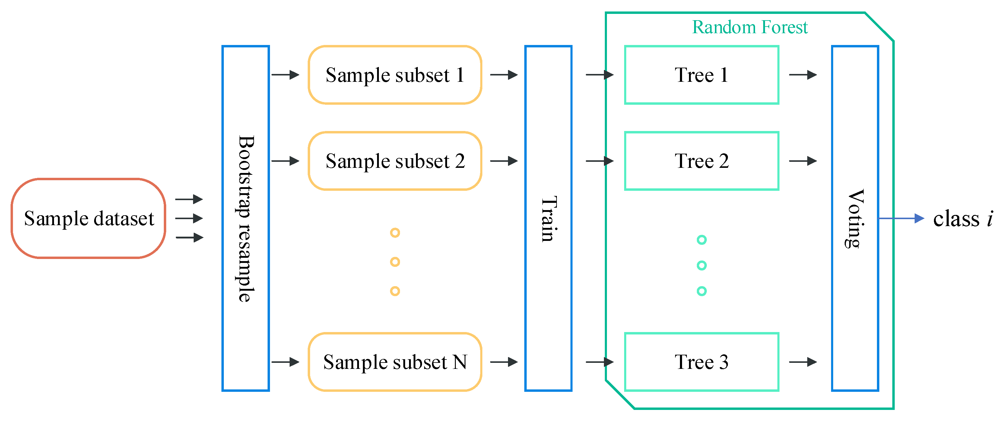
• For a decision tree, randomly sample N times from the sample dataset of size N with put-back, as the training subset of the tree.
• Randomly select m ($m=\sqrt{M}$) features from a total of M features as the set of features used for the nodes division of this tree.
• Using the CART (Classification and Regression Tree) algorithm to grow the tree completely without pruning.
• Repeat the above steps until all trees have been generated.

RF uses the bootstrap resampling technique in the process of tree generation, i.e., sampling with put-back. The probability that each sample in the sample set D is not sampled during the train subset generation of each decision tree is ${\left(1-1/N\right)}^N$, and N is the number of samples in D. When N is large enough then [31].

$$\underset{N\to \infty }{\lim }{\left(1-1/N\right)}^N=1/e\approx 0.368$$

(5)

Thus for each tree, about 36.8% of samples in the sample dataset are not used in the generation of that tree, and these samples are called Out-Of-Bag (OOB) data for the tree, and the performance of the model can be estimated using the OOB data, i.e., OOB estimation.

The calculation of feature importance based on OOB estimation is implemented by comparing the classification accuracy of features before and after adding interference [32]. For sample subset i (i = 1, 2, …, N_tree), the importance score D_j of feature X_j (j = 1, 2, …, M) is calculated according to the following steps.

• Set the decision tree T_i and the OOB data $L_i^{oob}$ to correspond to i.
• Use T_i to classify $L_i^{oob}$ and count the number of correctly classified $R_i^{oob}$.
• Perturb the value of X_j in $L_i^{oob}$, and mark the dataset after the perturbation as $L_{ij}^{oob}$. Use T_i to classify $L_{ij}^{oob}$ and count the number of correctly classified $R_{ij}^{oob}$.
• For i = 2, 3, …, N_tree, repeat steps 1~3.
• The importance score D_j of the feature X_j is calculated by the following formula:

  $$D_j=\frac{1}{N_{tree}}{\displaystyle \sum _{i=1}^{N_{tree}}\left(R_i^{oob}-R_{ij}^{oob}\right)}$$

  (6)

The steps of feature selection based on importance score are as follows [13]:

• Scale the importance score of each feature to the range of 0~1, and sort from largest to smallest.
• Generate an RF model using features with a score of 1.
• Generate other RF models based on the following two rules by adding the less important features in turn:

  (1)

  Add no more than three features each time.

  (2)

  The maximum difference between the importance scores of the features added each time should be less than 0.2.

The performance of the models is evaluated by calculating the classification accuracy and Kappa coefficient. The model with the performance is similar to the model trained with all features and the least features is the model generated by the best-preferred features.

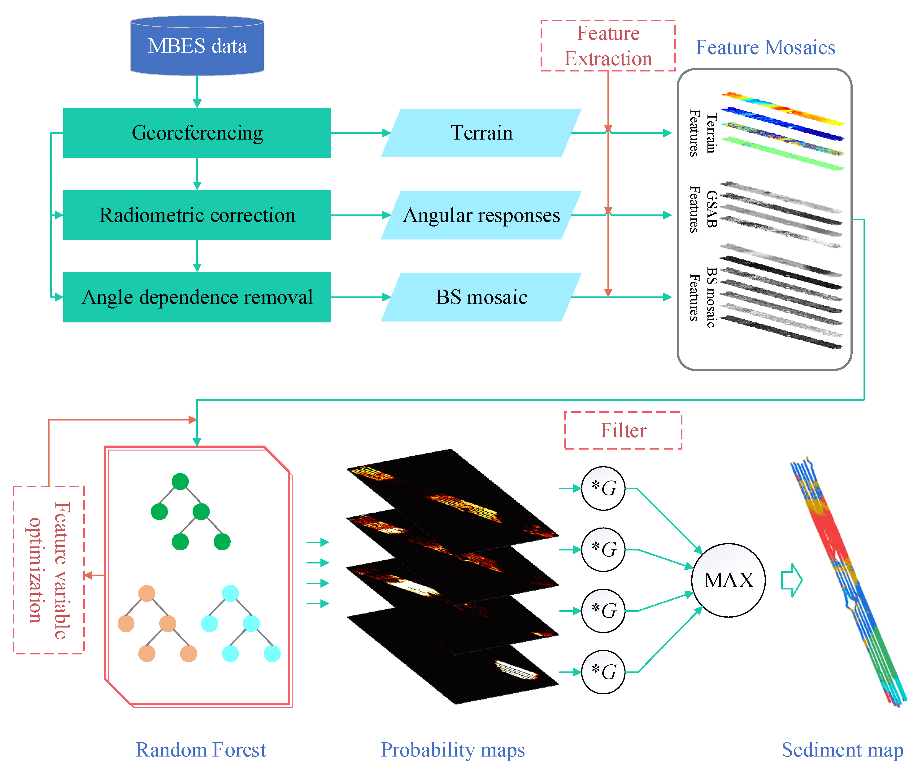
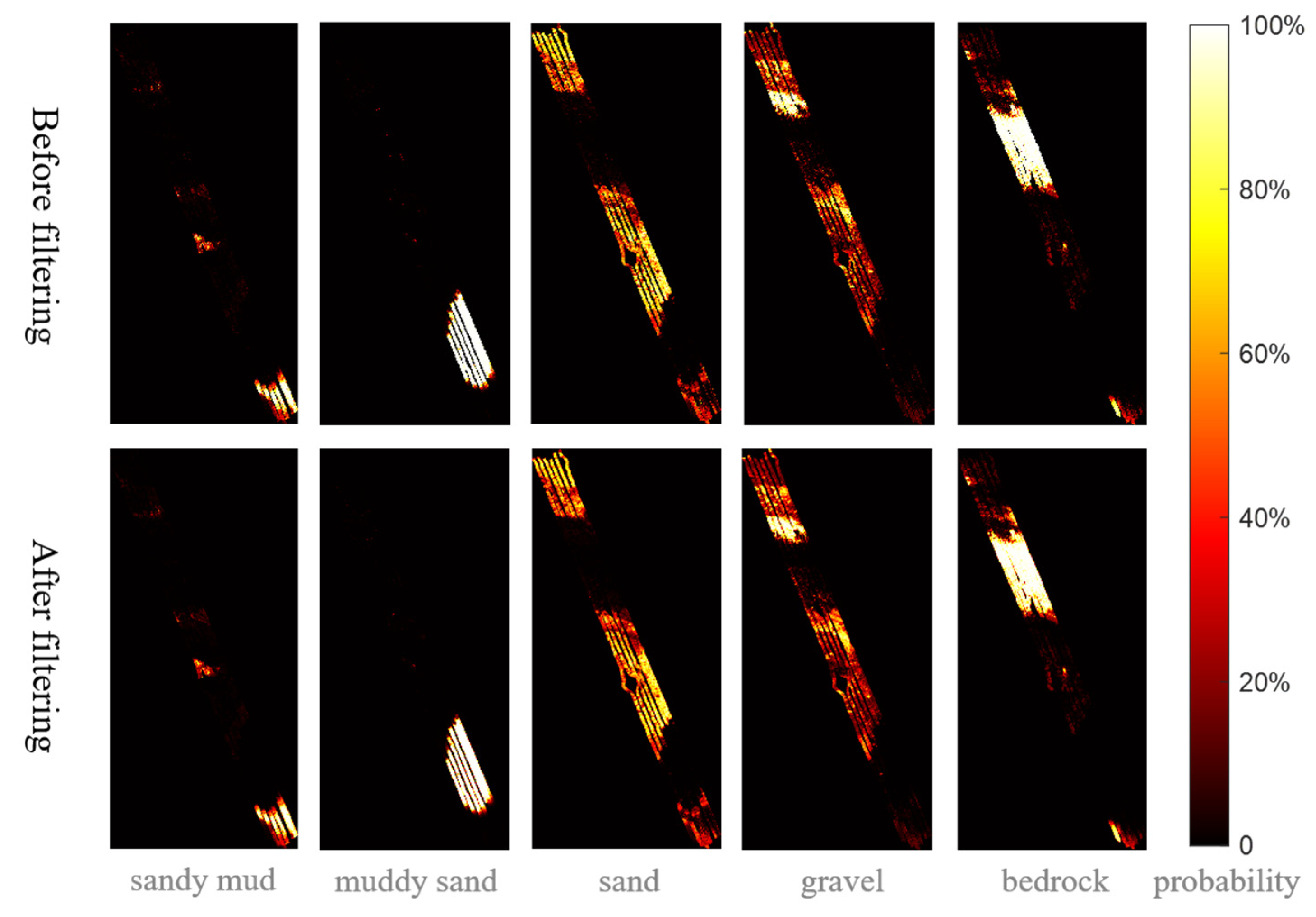
2.4. Probability Map Denoising and Sediment Mapping

The classification model can obtain the probability of each input feature vector belonging to each category by the voting method. We can get N_class (N_class is the total number of sediment types) probability maps by the following steps:

• Input the feature vector to be classified into the trained RF model, and calculate the probability $p_i$ (i = 1, 2, …, N_class) belonging to each type of sediment.
• Encode $p_i$ to generate a probability map $P_i$ according to the geographic location of the feature vector.

The MBES data are degraded by various types of noise and reverberation, and the obtained terrain and BS contain many outliers, which will cause a lot of isolated points in sediment maps with pixel-oriented classification. The computational effort of the methods of filtering the features increases as the number of features increases and the final result cannot be predicted. Although the image filtering methods can eliminate the isolated noise in the sediment map, the category values in the sediment map are discrete, so it is difficult to obtain a good filtering performance. Therefore, we use a denoising method for sediment maps with probability maps.

Gaussian filtering is chosen because it uses a weighted average to denoise, which accords with the neighborhood correlation of sediment distribution. We filter $P_i$ to obtain the filtered probability map $P_i^G$ with a two-dimensional Gaussian filter. Finally, we synthesize all $P_i^G$ to generate the sediment map (the sediment type corresponding to the maximum probability pimax of each pixel is the sediment type to which the pixel belongs).

3. Experimental Section

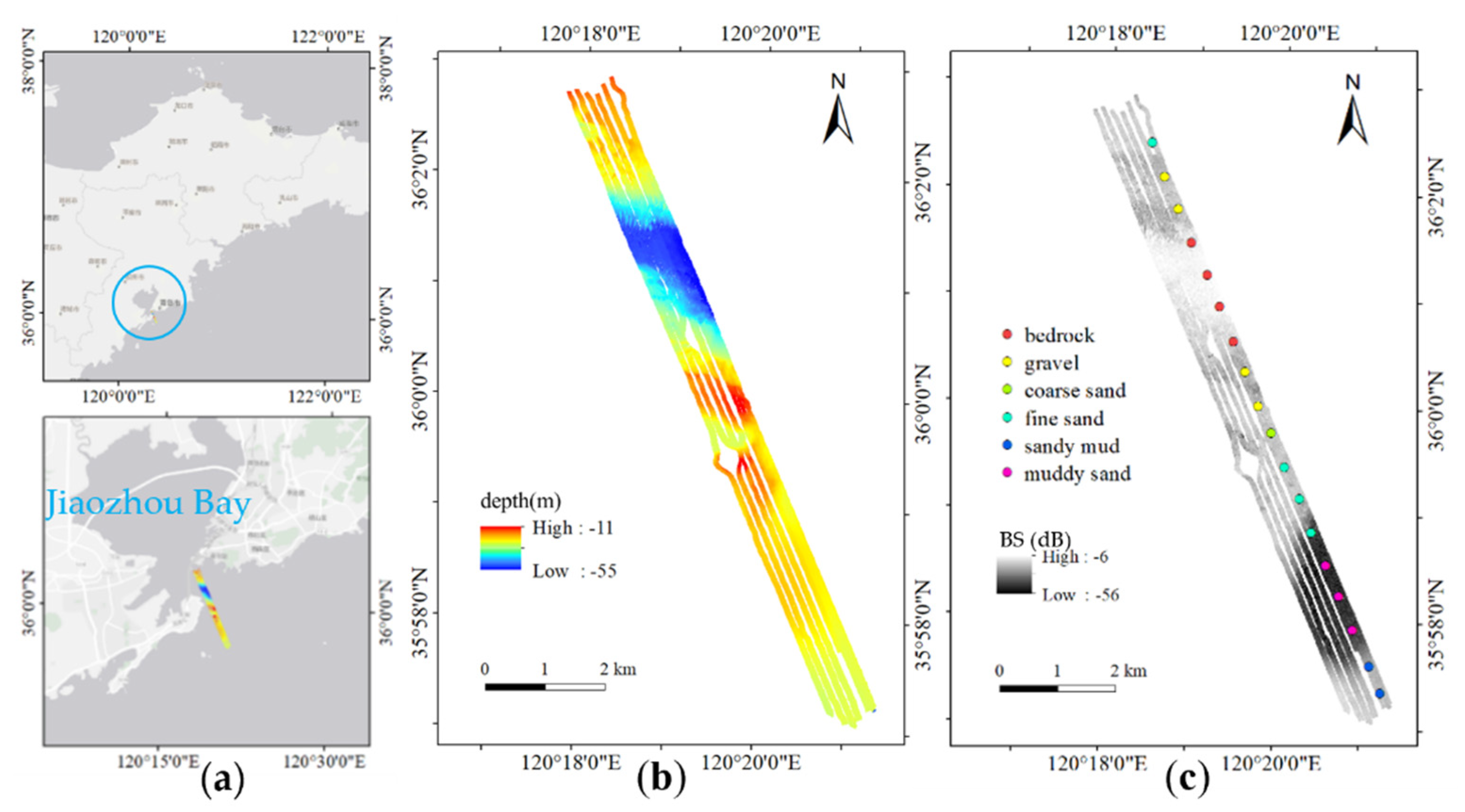
3.1. Data

The study area is located in the central Yellow Sea, south coast of Jiaodong Peninsula, and the entrance of Jiaozhou Bay, China. Jiaozhou Bay is a semi-enclosed bay in the shape of a trumpet. The various underwater geomorphic types and rich seabed sediment types in Jiaozhou Bay include chalky clay, clayey silt, muddy sand, sandy mud, silt, coarse sand, gravel, mudstone, and bedrock, which is conducive to the study of sediment classification [33,34]. We use 16 lines measured by Kongsberg Simrad EM3002 multibeam system in Jiaozhou Bay in 2002, with a total length of 66 km and a coverage area of 6.6 km². The operating frequency of EM3002 is 300 kHz, the beam angle is 1.5° × 1.5°, the equipment adopts equal angle mode, the sector opening angle is about 140°, and there are about 116 single beam points per ping. The location of the survey area is shown in Figure 5a. The topography of the survey area is shown in Figure 5b, and the depth ranges from 11 to 55 m. Within the survey area, there are 18 sediment samples obtained with the box sampler during the same period, and the sampling locations are shown in Figure 5c, which are uniformly distributed along the main direction of the survey area, and the sediment samples include 3 muddy sand samples, 2 sandy mud samples, 4 fine sand samples, 1 coarse sand sample, 4 gravel samples, and 4 bedrock samples. Since there is only one coarse sand sample, we treat it as sand together with fine sand. In order to make the sample size meet the requirements of the algorithm, we select pixels near sediment samples and divide them into the training samples and the test samples. About 500 pixels of each sediment type constitute the training set, and about 200 pixels constitute the test set.

3.2. Sediment Classification

The raw data is processed according to the MBES data processing method to obtain the seafloor topography (Figure 5b), BS, and BS mosaic (Figure 5c). We construct a sample dataset, extract features, build the classification model, and denoise the sediment map with these three types of MBES data and sampling information.

3.2.1. Feature Extraction

A total of 15-dimensional features such as AR features, terrain features, and texture features are extracted using the method in Section 2.1 and Section 2.2 using AR data, terrain data, and BS mosaic, and the mosaics generated by each type of feature are shown in Figure 6.

MBES often operates with transmitting or receiving gain to improve the signal-noise ratio, enhancing the robustness of topographic measurement, yet adding complex beam patterns to the BS. The data in the survey area also contains a beam pattern, as shown by the bulge in the ARC near 20° and abnormally high values beyond 55° in Figure 7. We use a sliding window of size 30 pings, and the port and starboard are fitted to the GSAB model using the method in Section 2.1 to obtain ARCs and extract AR features.

Figure 7 shows the comparison of the ARC fitting results between the least squares method and the Huber regression method for the regions with high, medium, and low-level BS. Regions 1, 2, and 3 on the left are the regions with high, medium, and low-level BS, respectively, and the fitting results of ARCs for each region correspond to plots 1, 2, and 3 on the right. It can be found that the fitting results of the two methods within 30° do not differ significantly, but the fitting results of the least squares method in the decay rate at the edge beams are significantly lower than the Huber regression method due to the influence of beam pattern at the edge beams. Judging from the trend of BS variation in the range of 30° to 55° without the influence of beam pattern, the fitting results of the Huber regression method are more similar to the trend of the true ARCs, and therefore, the Huber regression method is considered to be more robust in fitting the ARC with the influence of beam pattern.

3.2.2. Feature Selection and Sediment Classification

Xue Ji et al. [9] analyzed how the parameters of RF were selected in MBES sediment classification. Oshiro T.M. et al. [35] discussed the effect of the number of trees on the performance of RF. The larger the number of decision trees N_tree, the higher the accuracy of the model, but the higher the computational cost and the risk of overfitting. Increasing the number of random features m used to construct the decision tree can improve the accuracy of the model, but it reduces the diversity of decision trees and increases the risk of overfitting [32]. Taking into account factors such as model accuracy and computational cost, setting N_tree = 200 (to minimize errors rates), m = $\sqrt{M}$ (M is the total number of features) is suitable for establishing a random forest model for sediment classification [13]. Input the training dataset to train the model, and use OOB estimation to obtain the classification accuracy and the feature importance.

Table 2. Feature sets of different models and classification performance.

	Model 1	Model 2	Model 3	Model 4	Model 5
A	√			√	√
B	√			√	√
C	√		√	√	√
D	√				√
depth	√	√	√	√	√
slope	√		√	√	√
aspect	√				√
curvature	√
BS	√			√	√
Con	√
Asm	√
Ent	√				√
Cor	√
Hom	√
Dis	√
sandy mud	0.96	0.86	0.96	0.97	0.96
muddy sand	0.98	0.56	0.98	0.99	0.99
sand	0.84	0.41	0.79	0.86	0.84
gravel	0.93	0.51	0.86	0.87	0.89
bedrock	0.98	0.8	0.95	0.97	0.98
Overall accuracy	93.7%	63.2%	91.2%	93.3%	93.4%
Kappa	0.92	0.54	0.89	0.92	0.92

shows the classification performance of different feature sets in the feature selection process. Model 1 is the classification performance that integrates AR features, terrain features, and BS mosaic features. The importance score of features based on Model 1 is shown in Figure 8. Train the model with the highest-scoring feature depth to get Model 2, then other features are gradually added to build the classification models according to the feature selection method in Section 2.3 to obtain Model 3~Model 5, and compare the performance of models to determine the best feature set.

As shown in Table 2, the overall classification accuracy of Model 4 is 93.3%, and the Kappa coefficient is 0.92, which is close to the performance of Model 1, and Model 4 uses fewer features than Model 5. Therefore, the features of Model 4 are considered the best-preferred features, i.e., the parameters A, B, and C of GSAB, depth, slope of terrain features, and BS as features to construct the classification model.

3.2.3. Denoising

The probability maps of various sediments are obtained based on the above model for sediment classification, and a Gaussian convolution kernel is constructed to filter the probability maps, and the probability maps and sediment maps before and after filtering are shown in Figure 9 and Figure 10. Gaussian filtering utilizes the neighborhood information and can effectively filter out isolated abnormal probability pixels without seriously affecting the regional sediments of the probability maps. As shown in Figure 10, the regional sediments are preserved as shown in the detailed comparison of area 1. Burrs on the contours of the bedrock in Area 1 are effectively eliminated. The detailed comparison of Area 2 shows that the isolated sediment areas consisting of a single pixel, or several pixels are filtered, such as the scatters of sandy mud, gravel, and bedrock. Area 3 shows that the outlines at the sediment boundary are well preserved without serious distortion. The originally chaotic outlines of gravel in the bottom-left corner in Area 3 are more clear after processing.

3.3. Validity of AR Features Extracted by the GSAB Model

The method in this paper (Method 4) is compared with the following three methods:

Method 1: Gaussian mixture model [36];

Method 2: the sediment classification method with terrain features and BS mosaic features;

Method 3: the sediment classification method with AR features (mean, slope, kurtosis, skewness), terrain features, and BS mosaic features.

The performance of the four methods is shown in

Table 3. Classification accuracy of four methods.

	Method 1	Method 2	Method 3	Method 4
sandy mud	0.36	0.92	0.96	0.96
muddy sand	0.99	0.97	0.98	0.98
sand	0.55	0.75	0.77	0.84
gravel	0.39	0.85	0.86	0.93
bedrock	0.99	0.97	0.99	0.98
overall accuracy	62.2%	89.6%	91.3%	93.3%
kappa	0.52	0.87	0.89	0.92

and the sediment maps are shown in Figure 11. It can be seen that:

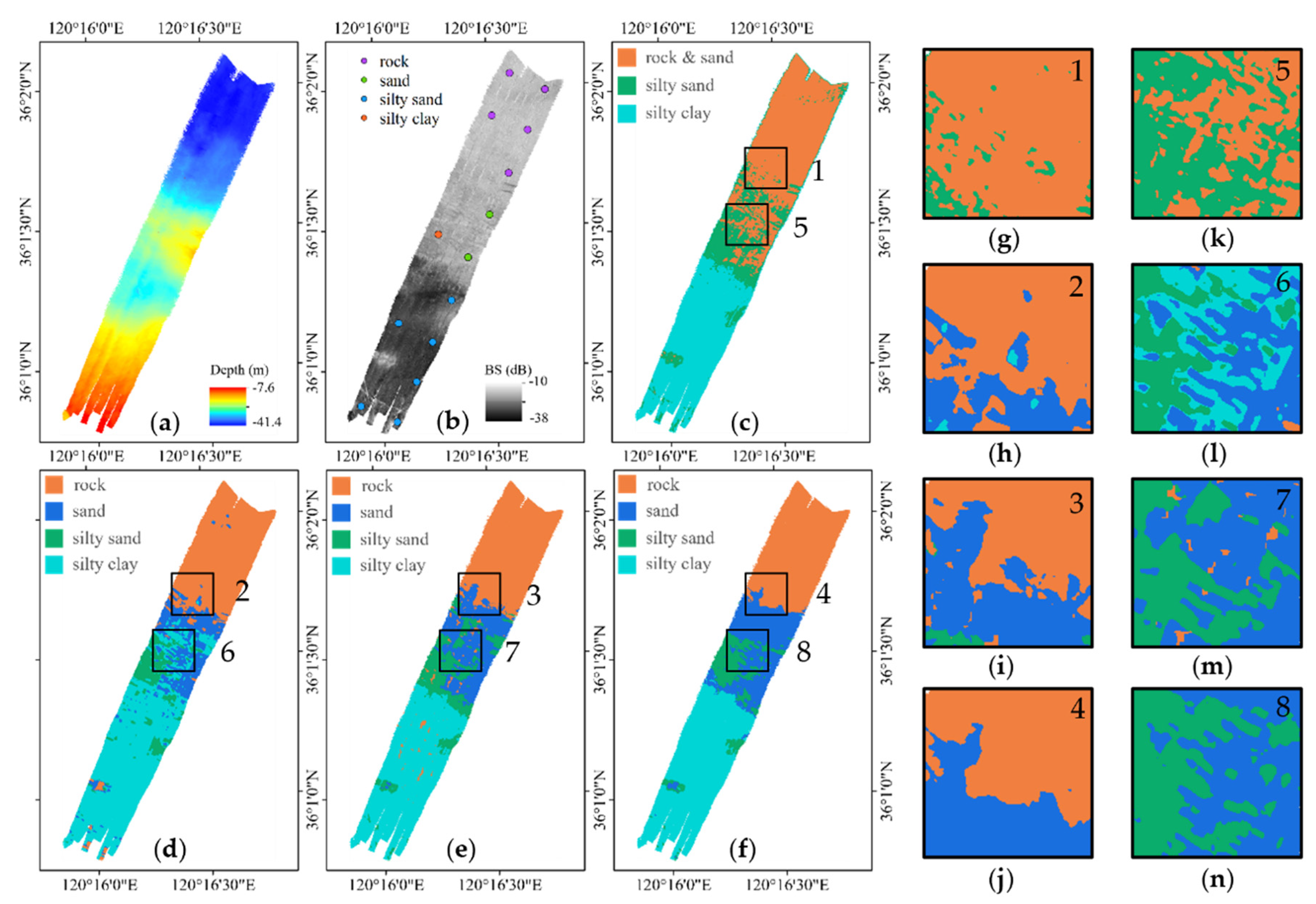
• Classification based on the statistical property of BS (Method 1), due to the single feature and the sensitivity of statistical property to factors of abnormal echoes and beam pattern residual, the classification model has a serious inadequacy of ability to distinguish sediments with small differences in BS, such as sandy mud, sand, and gravel, and the classification accuracy is low. For instance, the sandy mud in area 1 in Figure 11 is misclassified as gravel.
• Classification based on topographic and geomorphic features (Method 2) improved the ability to classify different sediments. It is shown that topographic and geomorphic features are necessary for sediment classification. However, the classification accuracy of sand is still not high, mainly due to the limitations of the classification capability. Furthermore, in confounding areas of multiple sediments, such as in area 2, the boundaries of the sediment in the sediment map of Method 2 are very messy.
• Classification with the addition of AR features (Method 3) has improved the results relative to Method 2, indicating that the AR features reflect the sediment properties better relative to other features, but are still influenced by the less robustness of the AR features extraction method. For instance, in area 3, a portion of sand is misclassified as gravel, resulting in a large area of sand scattered with some gravel in the sediment map of Method 3.
• Classification using the GSAB model parameters as AR features (Method 4) has the highest accuracy, indicating that the AR features extracted from the GSAB model can better describe the sediment properties and proves the validity of the method in this paper. In the sediment map of Method 4, the areas 4, 5, and 6 correspond to the areas 1, 2, and 3 of other methods, respectively, and have a more correct sediment distribution, more reasonable boundaries, and fewer sediment impurities.

Convert the parameter units using Formula (7) and calculate the average value of the GSAB model parameters of various sediments classified by Method 4, and draw various sediment ARCs, as shown in Figure 12 and

Table 4. The GSAB model parameters of various sediments.

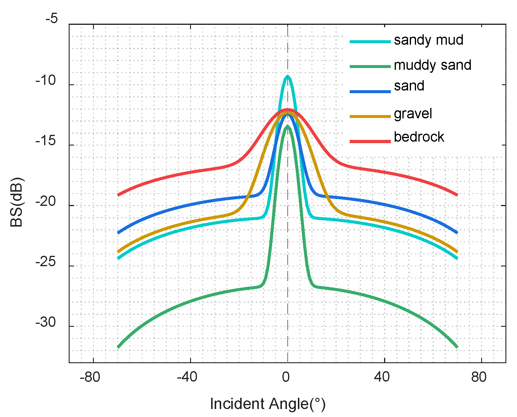
	A0 (dB)	B0 (°)	C0 (dB)	D0
sandy mud	−9.60	2.849	−20.99	0.73
muddy sand	−13.65	2.941	−26.65	1.09
sand	−13.42	3.868	−19.14	0.67
gravel	−12.99	7.012	−20.53	0.71
bedrock	−13.92	8.404	−16.62	0.54

. It can be found that these parameters can effectively distinguish different sediment types.

$$\begin{array}{l}{A}^0=10\log A\hspace{1em}\left(\mathrm{dB}\right)\\ B^0=\frac{B\times 180}{\pi }\hspace{1em}\hspace{1em}(°)\\ C^0=10\log C\hspace{1em}\left(\mathrm{dB}\right)\\ D^0=D\end{array}$$

(7)

A⁰ is the BS corresponding to the incident angle of 0°, that is, the peak value of the ARC. The A⁰ of sandy mud is significantly higher than the other four types of sediments, so A⁰ can distinguish sandy mud from other sediments.

B⁰ represents the angular range of the specular reflection area. The B⁰ of gravel and bedrock is significantly higher than other sediments, so B⁰ can distinguish gravel and bedrock from other sediments.

C⁰ indicates the average level of BS in the grazing angles. The C⁰ of muddy sand is significantly lower than that of other sediments, and that of bedrock is higher than that of other sediments, so C⁰ can distinguish muddy sand, bedrock, and other sediments.

D⁰ represents the decay rate of the BS in the grazing angles. D⁰ is larger for muddy sand and smaller for bedrock, so D⁰ can distinguish muddy sand, bedrock, and other sediments.

The GSAB model parameters distinguish sediments very accurately. The method in this paper also takes into account the topographic and geomorphic features, which significantly improves the ability to describe the sediment properties. In particular, the classification accuracy of sediments with small differences in BS, such as sand and gravel, is improved, and the overall classification accuracy is improved.

4. Discussion

4.1. Comparison of Results from Different Classifiers

Researchers have applied many classification algorithms to sediment classification, including unsupervised methods (SOM [37], ISOdata [38], HCA [39,40], etc.) and supervised methods (SVM [41], RF [8,13], BPNN [42], CNN [12], etc.). To prove the validity of our proposed method, we compare its classification results with those of other classifiers. An unsupervised image segmentation method with Convolutional Neural Networks based on Differentiable Feature Clustering [43] is used for sediment classification (hereinafter referred to as DFC). We also use Back-Propagation Neural Network (BPNN), Support Vector Machine (SVM) for classification as comparative experiments.

The sediment maps obtained by different classifiers are shown in Figure 13, and the classification accuracy is shown in

Table 5. Classification accuracy of different classifiers.

Methods	Categories	User’s Accuracy (%)	Producer’s Accuracy (%)	Average Accuracy (%)	Overall (%)	Kappa
DFC	muddy sand	94.6	100	97.3	81.9	0.75
	sand	54.6	60.9	57.8
	gravel & sandy mud	83.6	87.7	85.7
	bedrock	100	73.3	86.7
BPNN	sandy mud	95	83.2	89.1	84.2	0.8
	muddy sand	78.1	99	88.6
	sand	78.5	69.6	74.1
	gravel	78.7	77.4	78.1
	bedrock	92.9	92	92.5
SVM	sandy mud	86	96.3	91.2	86.3	0.83
	muddy sand	98	97.3	97.7
	sand	69.5	79.7	74.6
	gravel	83.6	66.3	75.0
	bedrock	97.2	92	94.6
Our Method	sandy mud	95.8	97	96.4	93.3	0.92
	muddy sand	98.6	97.4	98.0
	sand	84.5	84	84.3
	gravel	89.6	96.3	93.0
	bedrock	96.7	98.9	97.8

. On a larger scale, the prediction results given by four classification methods are generally consistent. However, there are still large differences in the local details. Based on the sample information, the categories clustered by DFC are correlated to the sediment types. Without training, DFC can not effectively take the advantage of differences in sediments, and grouped sandy mud and gravel into the same category, as area 5. In area 1, a large area of bedrock is misclassified as sand. In areas 2, 3, 6, and 7, the types and distribution of the sediment are generally consistent, but several small-scale sediments scatter in other sediments, such as several localized gravel areas in area 2 and sandy mud areas in area 3 scattered over the bedrock area. It is believed that these local sediments have been misclassified. In general, the classification result of the proposed method shows a more reasonable distribution of sediments, and the classification accuracy is the highest, reaching 93.3% in total.

We performed the same comparison using MBES data from another surveying area, namely Area-II. The terrain and BS mosaic obtained from the MBES data are shown in Figure 14. The sediment maps obtained from different classification methods are also shown in Figure 14, and the classification accuracy is shown in

Table 6. Classification accuracy of different classifiers in Area-II.

Methods	Categories	User’s Accuracy (%)	Producer’s Accuracy (%)	Average Accuracy (%)	Overall (%)	Kappa
DFC	rock & sand	89.8	73.3	81.55	82.1	0.72
	silty sand	62	81.7	71.85
	silty clay	95.2	100	97.6
BPNN	rock	95.2	100	97.6	83.7	0.78
	sand	85.4	69.5	77.45
	silty sand	97.6	68.3	82.95
	silty clay	67.4	96.7	82.05
SVM	rock	80	100	90	84.6	0.79
	sand	81.8	75	78.4
	silty sand	78.9	75	76.95
	silty clay	100	88.3	94.15
Our Method	rock	100	100	100	92.9	0.9
	sand	83.1	90	86.55
	silty sand	90.7	81.7	86.2
	silty clay	98.4	100	99.2

. The unsupervised DFC classifies this area into three categories, corresponding to rock and sand, silty sand, silty clay, respectively, and other methods obtain four types of sediment. Two areas in each sediment map are zoomed in for detailed comparison, as shown in Figure 14. The method we proposed shows good performance in noise reduction and the reliability of sediment boundaries because of the highest classification accuracy, the homogeneity inside the sediment, and clear boundaries of different categories.

4.2. Limitations

4.2.1. The Influence of Different Operation Modes on AR Feature Extraction

To ensure the quality of the sounding data and achieve high-precision, full-coverage measurement, the MBES will adopt the multi-sector transmission mode. For example, Kongsberg EM302 MBES has five operation modes: Shallow, Medium, Deep, Very Deep, and Extra Deep, and the operation mode can be automatically switched or manually set according to the water depth. A group of data may be obtained using different operation modes, i.e., different beam patterns contained in the backscatter data. The Huber regression method used in this paper to fit the GSAB model to extract AR features cannot eliminate the beam pattern. Therefore, there may be differences in AR features of the same sediment under different operation modes, which will affect the classification results. To solve this problem, the beam pattern elimination method proposed in reference [44] can be used first. This method combines the backscatter data of homogeneous sediment region and the GSAB model to iteratively extract the beam pattern residuals and apply the correction to other data in the same beam pattern to eliminate the beam pattern residuals.

4.2.2. The Influence of Mixed Sediments in Ping

BS of multiple types of sediment may exist in one ping in areas with complex sediments or at the boundary of different sediments. In this case, one set of ARC parameters cannot correspond to the characteristic of one sediment, which leads to an inaccurate description of the sediment by the AR features, which affects the classification accuracy. Especially when there is a type of sediment with strong scattering ability at the edge beam, the BS of the edge beam in this region is higher, but the process of extracting AR features in this paper suppresses the beam pattern while also biasing the AR feature values for this case. Topographic features and BS mosaic features can make up for the shortage of AR features, and the method in this paper is still valid for mixed sediments within one ping which can be effectively classified by topographic features or BS mosaic features. If the topographic features or BS mosaic features are weak in classifying mixed sediments within one ping, it is necessary to consider an iterative method to conduct feature extraction and classification. Each time, AR features are extracted using all AR data of the same type of sediment based on the last classification result to realize the classification from coarse to fine.

4.2.3. The Influence of Abnormal Data on Feature Extraction

The bottom detection algorithm of MBES sometimes has errors, not only in single beam point data but also in regional data, especially in the deep sea, which may lead to several beams or even ping data exceptions, resulting in regional exceptions in DEM and BS mosaic. For errors caused by a single beam point, the Huber regression and probability map filtering used in this paper can effectively eliminate them. For errors caused by local beam points, the extracted feature values are biased, resulting in incorrect classification results, and cannot be removed effectively by the filtering method because they are not pixel-level errors. To solve this problem, abnormal regions can be deleted in data preprocessing, and the sediment of these regions can be interpolated according to the distribution of surrounding sediments after classification.

5. Conclusions

Conventional sediment classification methods based on MBES data have low accuracy since the correlation between features and sediment has not been fully considered, thus, this paper developed a new seabed sediment classification method. By combining the GSAB model and Huber regression to fit ARC, the AR features obtained are less influenced by noise, and accurately reflect the differences in sediment types. Probability maps are filtered by a Gaussian filter to solve tiny isolated blocks in sediment maps. 6-D features are selected for classification using the RF algorithm, and high classification accuracy is obtained. Experiments in Jiaozhou Bay and Area-II have achieved an overall accuracy of 93.3% and 92.9%, respectively, which demonstrates the validity of this seabed sediment classification method. Comparison experiments demonstrated the superiority of the proposed method, and sediment maps obtained perform well in noise suppression and outline retention.

References

- Panneerselvam, B.; Muniraj, K.; Thomas, M.; Ravichandran, N.; Bidorn, B. Identifying Influencing Groundwater Parameter on Human Health Associate with Irrigation Indices Using the Automatic Linear Model (ALM) in a Semi-Arid Region in India. Environ. Res. 2021, 202, 111778. [Google Scholar] [CrossRef] [PubMed]
- Ramalingam, S.; Panneerselvam, B.; Kaliappan, S.P. Effect of High Nitrate Contamination of Groundwater on Human Health and Water Quality Index in Semi-Arid Region, South India. Arab. J. Geosci. 2022, 15, 242. [Google Scholar] [CrossRef]
- Fonseca, L.; Calder, B. Geocoder: An Efficient Backscatter Map Constructor. In Proceedings of the U.S. Hydro 2005 Conference, San Diego, CA, USA, 22 September 2005. [Google Scholar]
- TANG, Q.H.; JI, X.; DING, J.S.; ZHOU, X.H.; LI, J. Research Progress and Prospect of Acoustic Seabed Classification Using Multibeam Echo Sounder. Adv. Mar. Sci. 2019, 37, 1–10. [Google Scholar] [CrossRef]
- Preston, J. Automated Acoustic Seabed Classification of Multibeam Images of Stanton Banks. Appl. Acoust. 2009, 70, 1277–1287. [Google Scholar] [CrossRef]
- Brown, C.J.; Todd, B.J.; Kostylev, V.E.; Pickrill, R.A. Image-Based Classification of Multibeam Sonar Backscatter Data for Objective Surficial Sediment Mapping of Georges Bank, Canada. Cont. Shelf Res. 2011, 31, S110–S119. [Google Scholar] [CrossRef]
- Koop, L.; Snellen, M.; Simons, D.G. An Object-Based Image Analysis Approach Using Bathymetry and Bathymetric Derivatives to Classify the Seafloor. Geosciences 2021, 11, 45. [Google Scholar] [CrossRef]
- Shang, X.; Robert, K.; Misiuk, B.; Mackin-McLaughlin, J.; Zhao, J. Self-Adaptive Analysis Scale Determination for Terrain Features in Seafloor Substrate Classification. Estuar. Coast. Shelf Sci. 2021, 254, 107359. [Google Scholar] [CrossRef]
- Ji, X.; Yang, B.; Tang, Q. Seabed Sediment Classification Using Multibeam Backscatter Data Based on the Selecting Optimal Random Forest Model. Appl. Acoust. 2020, 167, 107387. [Google Scholar] [CrossRef]
- Hughes Clarke, J.E.; Mayer, L.A.; Wells, D.E. Shallow-Water Imaging Multibeam Sonars: A New Tool for Investigating Seafloor Processes in the Coastal Zone and on the Continental Shelf. Mar. Geophys. Res. 1996, 18, 607–629. [Google Scholar] [CrossRef]
- JIN, S.; LI, J.; WU, Z.; BIAN, G.; CUI, Y. 3D Histogram of Backscatter Strength for Seafloor Substrates Classification. Acta Geod. Cartogr. Sin. 2019, 48, 124–131. [Google Scholar] [CrossRef]
- YANG, F.; ZHU, Z.; LI, J.; FENG, C.; XING, Z.; WU, Z. Seafloor Classification Based on Combined Multibeam Bathymetry and Backscatter Using Deep Convolution Neural Network. Acta Geod. Cartogr. Sin. 2021, 50, 71–84. [Google Scholar] [CrossRef]
- Hasan, R.C.; Ierodiaconou, D.; Laurenson, L.; Schimel, A. Integrating Multibeam Backscatter Angular Response, Mosaic and Bathymetry Data for Benthic Habitat Mapping. PLoS ONE 2014, 9, e97339. [Google Scholar] [CrossRef] [Green Version]
- Hellequin, L.; Lurton, X.; Augustin, J.M. Postprocessing and signal corrections for multibeam echosounder images. In Proceedings of the Oceans’97, MTS/IEEE Conference, Halifax, NS, Canada, 6–9 October 1997; pp. 23–26. [Google Scholar] [CrossRef]
- JIN, S.; XIAO, F.; BIAN, G.; WANG, M.; SUN, W. A Method for Extracting Seabed Feature Parameters Based on the Angular Response Curve of Multibeam Backscatter Strength. GEOMATICS Inf. Sci. WUHAN UNIVERS 2014, 39, 1493–1498. [Google Scholar] [CrossRef]
- Hughes Clarke, J.E.; Li, M.Z.; Sherwood, C.R.; Hill, P.R. Optimal use of multibeam technology in the study of shelf morphodynamics. In Sediments, Morphology and Sedimentary Processes on Continental Shelves: Advances in Technologies, Research and Applications, 1st ed.; International Association of Sedimentologists: Gent, Belgium, 2013; pp. 3–28. [Google Scholar] [CrossRef]
- Diesing, M.; Mitchell, P.; Stephens, D. Image-Based Seabed Classification: What Can We Learn from Terrestrial Remote Sensing? ICES J. Mar. Sci. J. du Cons. 2016, 73, 2425–2441. [Google Scholar] [CrossRef]
- Schimel, A.C.G.; Beaudoin, J.; Parnum, I.M.; Le Bas, T.; Schmidt, V.; Keith, G.; Ierodiaconou, D. Multibeam Sonar Backscatter Data Processing. Mar. Geophys. Res. 2018, 39, 121–137. [Google Scholar] [CrossRef]
- Lurton, X.; Lamarche, G. (Eds.) Backscatter Measurements by Seafloor-Mapping Sonars. Guidelines and Recommendations. 2015. Available online: https://niwa.co.nz/static/BWSG_REPORT_MAY2015_web.pdf (accessed on 15 September 2021).
- Augustin, J.M.; Lurton, X. Image amplitude calibration and processing for seafloor mapping sonars. In Proceedings of the IEEE Oceans’ 2005 European Conference, Brest, France, 20–23 June 2005; pp. 698–701. [Google Scholar]
- Augustin, J.; Edy, C.; Savoye, B.; Le Drezen, E. Sonar mosaic computation from multibeam echo sounder. In Proceedings of the OCEANS’94, Oceans Engineering for Today’s Technology and Tomorrow’s Preservation, Brest, France, 13–16 September 1994; Volume 432, pp. II/433–II/438. [Google Scholar] [CrossRef]
- Lamarche, G.; Lurton, X.; Verdier, A.-L.; Augustin, J.-M. Quantitative Characterisation of Seafloor Substrate and Bedforms Using Advanced Processing of Multibeam Backscatter—Application to Cook Strait, New Zealand. Cont. Shelf Res. 2011, 31, S93–S109. [Google Scholar] [CrossRef] [Green Version]
- Brekhovskikh, L.M.; Lysanov, Y.P. Fundamentals of Ocean Acoustics, 3rd ed.; Springer: New York, NY, USA, 2003. [Google Scholar] [CrossRef]
- Lurton, X.; Jackson, D.R. An Introduction to Underwater Acoustics. J. Acoust. Soc. Am. 2004, 115, 443. [Google Scholar] [CrossRef] [Green Version]
- Huber, P.J. Robust Statistics. In International Encyclopedia of Statistical Science; Springer: Berlin/Heidelberg, Germany, 2011; pp. 1248–1251. [Google Scholar]
- Colenutt, A.; Mason, T.; Cocuccio, A.; Kinnear, R.; Parker, D. Nearshore Substrate and Marine Habitat Mapping to Inform Marine Policy and Coastal Management. J. Coast. Res. 2013, 165, 1509–1514. [Google Scholar] [CrossRef]
- Cui, X.; Liu, H.; Fan, M.; Ai, B.; Ma, D.; Yang, F. Seafloor Habitat Mapping Using Multibeam Bathymetric and Backscatter Intensity Multi-Features SVM Classification Framework. Appl. Acoust. 2021, 174, 107728. [Google Scholar] [CrossRef]
- Haralick, R.M.; Shanmugam, K.; Dinstein, I. Textural Features for Image Classification. IEEE Trans. Syst. Man. Cybern. 1973, 6, 610–621. [Google Scholar] [CrossRef] [Green Version]
- Baraldi, A.; Panniggiani, F. An Investigation of the Textural Characteristics Associated with Gray Level Cooccurrence Matrix Statistical Parameters. IEEE Trans. Geosci. Remote Sens. 1995, 33, 293–304. [Google Scholar] [CrossRef]
- Liaw, A.; Wiener, M. Classification and regression by randomForest. R News 2002, 2, 18–22. [Google Scholar]
- FANG, K.; WU, J.; ZHU, J.; SHIA, B. A Review of Technologies on Random Forests. Stat. Inf. FORUM 2011, 26, 32–38. [Google Scholar] [CrossRef]
- YAO, D.; YANG, J.; ZHAN, X. Feature Selection Algorithm Based on Random Forest. J. Jilin Univ. Technol. Ed. 2014, 44, 142–146. [Google Scholar] [CrossRef]
- Folk, R.L.; Andrews, P.B.; Lewis, D.W. Detrital Sedimentary Rock Classification and Nomenclature for Use in New Zealand. New Zeal. J. Geol. Geophys. 1970, 13, 937–968. [Google Scholar] [CrossRef] [Green Version]
- Charoenlerkthawin, W.; Namsai, M.; Bidorn, K.; Rukvichai, C.; Panneerselvam, B.; Bidorn, B. Effects of Dam Construction in the Wang River on Sediment Regimes in the Chao Phraya River Basin. Water 2021, 13, 2146. [Google Scholar] [CrossRef]
- Oshiro, T.M.; Perez, P.S.; Baranauskas, J.A. How many trees in a random forest? In Machine Learning and Data Mining in Pattern Recognition (Lecture Notes in Computer Science); Perner, P., Ed.; Springer: Berlin/Heidelberg, Germany, 2012; pp. 154–168. [Google Scholar] [CrossRef]
- Simons, D.G.; Snellen, M. A Bayesian Approach to Seafloor Classification Using Multi-Beam Echo-Sounder Backscatter Data. Appl. Acoust. 2009, 70, 1258–1268. [Google Scholar] [CrossRef]
- Yu, X.; Zhai, J.; Zou, B.; Shao, Q.; Hou, G. A Novel Acoustic Sediment Classification Method Based on the K-Mdoids Algorithm Using Multibeam Echosounder Backscatter Intensity. J. Mar. Sci. Eng. 2021, 9, 508. [Google Scholar] [CrossRef]
- Calvert, J.; Strong, J.A.; Service, M.; McGonigle, C.; Quinn, R. An Evaluation of Supervised and Unsupervised Classification Techniques for Marine Benthic Habitat Mapping Using Multibeam Echosounder Data. ICES J. Mar. Sci. 2015, 72, 1498–1513. [Google Scholar] [CrossRef] [Green Version]
- Panneerselvam, B.; Muniraj, K.; Duraisamy, K.; Pande, C.; Karuppannan, S.; Thomas, M. An Integrated Approach to Explore the Suitability of Nitrate-Contaminated Groundwater for Drinking Purposes in a Semiarid Region of India. Environ. Geochem. Health 2022, 1–17. [Google Scholar] [CrossRef]
- Panneerselvam, B.; Muniraj, K.; Pande, C.; Ravichandran, N.; Thomas, M.; Karuppannan, S. Geochemical Evaluation and Human Health Risk Assessment of Nitrate-Contaminated Groundwater in an Industrial Area of South India. Environ. Sci. Pollut. Res. 2021, 1–18. [Google Scholar] [CrossRef] [PubMed]
- Hasan, R.C.; Ierodiaconou, D.; Monk, J. Evaluation of Four Supervised Learning Methods for Benthic Habitat Mapping Using Backscatter from Multi-Beam Sonar. Remote Sens. 2012, 4, 3427–3443. [Google Scholar] [CrossRef] [Green Version]
- Ji, X.; Yang, B.; Tang, Q. Acoustic Seabed Classification Based on Multibeam Echosounder Backscatter Data Using the PSO-BP-AdaBoost Algorithm: A Case Study from Jiaozhou Bay, China. IEEE J. Ocean. Eng. 2020, 46, 509–519. [Google Scholar] [CrossRef]
- Kim, W.; Kanezaki, A.; Tanaka, M. Unsupervised Learning of Image Segmentation Based on Differentiable Feature Clustering. IEEE Trans. Image Process. 2020, 29, 8055–8068. [Google Scholar] [CrossRef]
- LI, C. Study on Beam Patten Correction of Multi-Sector Multibeam Sonar and Seabed Sediment Classification. Master’s Thesis, Wuhan University, Wuhan, China, 2020. [Google Scholar]