Article

Shoreline Change from Optical and Sar Satellite Imagery at Macro-Tidal Estuarine, Cliffed Open-Coast and Gravel Pocket-Beach Environments

by
Maria Victoria Paz-Delgado
1,
Andrés Payo
2,*,
Alejandro Gómez-Pazo
3,
Anne-Laure Beck
4 and
Salvatore Savastano
5
1
Department of Applied Physics II, University of Malaga, 29071 Malaga, Spain
2
British Geological Survey, Natural Environmental Research Council, Keyworth NG12 5GG, UK
3
CRETUS Institute, University of Santiago de Compostela, 15701 Santiago de Compostela, Spain
4
ARGANS, Plymouth PL6 8BU, UK
5
IsardSAT Ltd., Guildford GU2 7YG, UK
*
Author to whom correspondence should be addressed.
J. Mar. Sci. Eng. 2022, 10(5), 561; https://doi.org/10.3390/jmse10050561
Submission received: 21 March 2022 / Revised: 12 April 2022 / Accepted: 12 April 2022 / Published: 20 April 2022

Abstract

:
Coasts are continually changing and remote sensing from satellite has the potential to both map and monitor coastal change at multiple scales. This study aims to assess the application of shorelines extracted from Multi-Spectral Imagery (MSI) and Synthetic Aperture Radar (SAR) from publicly available satellite imagery to map and capture sub-annual to inter-annual shoreline variability. This is assessed at three macro-tidal study sites along the coastline of England, United Kingdom (UK): estuarine, soft cliff environment, and gravel pocket-beach. We have assessed the accuracy of MSI-derived lines against ground truth datum tideline data and found that the satellite derived lines have the tendency to be lower (seaward) on the Digital Elevation Model than the datum-tideline. We have also compared the metric of change derived from SAR lines differentiating between ascending and descending orbits. The spatial and temporal characteristics extracted from SAR lines via Principal Component Analysis suggested that beach rotation is captured within the SAR dataset for descending orbits but not for the ascending ones in our study area. The present study contributes to our understanding of a poorly known aspect of using coastlines derived from publicly available MSI and SAR satellite missions. It outlines a quantitative approach to assess their mapping accuracy with a new non-foreshore method. This allows the assessment of variability on the metrics of change using the Open Digital Shoreline Analysis System (ODSAS) method and to extract complex spatial and temporal information using Principal Component Analysis (PCA) that is transferable to coastline evolution assessments worldwide.

1. Introduction

Coasts are continually changing from the influence of natural processes and human interaction. The scale by which the coastal environment is modified ranges from microscopic (grains of sand) to global (changes in sea level). Projected changes and risks to people, ecosystems, and the physical environment represents a growing concern worldwide [1]. Being able to quantify physical coastal changes and its response to human actions is key to understanding the dynamic of the coast and to anticipate future behaviors, helping to make better informed planning decisions. The rates of physical change to coastlines can be expressed [2] in different units but rate of change is often used synonymously with coastline change, and thus expressed in m/year. The coastline, though strictly defined as the intersection of water and land surfaces, for practical purposes, the dynamic nature of this boundary and its dependence on the temporal and spatial scale at which it is being considered results in the use of a range of shoreline indicators which can be observed using different techniques and technologies [3,4]. Hereafter, we will use the term coastline and shoreline as equivalent generic names for the land and ocean water boundary. Earth Observations (EO) from satellites provide a potentially rich source of long-term historical shoreline datasets across spatial scales, ranging from local studies to global applications such as the work done by [5,6] to undertake a global-scale assessment of yearly shoreline change rates using optical multi-spectral images from different satellite missions. For a recent comprehensive review of a range of the methods available for shoreline extraction from and discussion of why some shoreline features have been identified using multispectral satellite imagery and others not, we refer the reader to [7]. Extending beyond the present focus of optical multi-spectral imagery and changes in annual mean shoreline position and estimation of long-term trends, the full exploitation of the extensive public satellite imagery applied to both short-term to seasonal timescales, as well as to annual variability and longer-term trends, is yet to be fully investigated and reported. Previous analysis [8] has demonstrated that satellite-derived shorelines spanning the past 30 years can be used to explore and quantify intra- and inter-annual shoreline behaviour at a number of beaches with micro tidal range (<4 m) around the world using optical Multi Spectral Images (MSI). To the best knowledge of the authors, there are no similar analyses done using coastlines derived from Synthetic Aperture Radar (SAR) images.
MSI and SAR satellite imagery captures data at different frequency bandwidths, which had implications for the changes that are able to detected. MSI captures the data in the optical bandwidth, using a different number of bands and the resolution of each band. MSI imagery uses less than 100 bands with a radiometer dedicated for each band tuned to the central wavelength. For instance, LANDSAT-8 is a multi-spectral system with 11 bands measuring all the way from 0.43 μm to 12.51 μm in discrete steps with resolutions varying from 15–100 m depending on the application. Since different materials reflect and absorb differently at different wavelengths, the reflectance spectrum of a material is a plot of the fraction of incoming solar radiation reflected as a function of the incident wavelength, which serves as a unique spectral signature for the material. Unlike optical technology, SAR can “see” through darkness, clouds, and rain, detecting changes in habitat, levels of water and surface soil moisture, effects of natural or human disturbance, and changes in the Earth’s surface after events such as earthquakes or sinkhole openings. The SAR signal is sensitive towards both the dielectric and geometric configuration of the target. Since the SAR wavelength is the same order of magnitude as the dimensions of real-life targets, interaction with the incoming signal is prominent. Targets whose dimensions are smaller relative to the imaging wavelength are perceived as smooth targets and therefore the scattering from a resolution cell containing such targets is relatively homogeneous. All SAR satellites travel from the North Pole towards the South Pole for half of their trajectory. This direction is referred to as their descending orbit. Conversely, when satellites travel from the South towards the North Pole, it is said to be in the ascending orbit. The same area is revisited along the two orbits. Consequently, ascending and descending images are collected over the same area.
The aim of this study is to investigate and compare the information contained on historical shorelines extracted from satellite MSI and SAR imagery in three macro-tidal (>4 m) coastal environments: estuarine, soft cliff environment, and gravel barrier beach. We use the Principal Component Analysis (PCA) (also referred to as Empirical Orthogonal Functions (EOFs)) [9] to extract the main temporal and spatial characteristics of the shoreline variability derived from MSI and SAR imagery. We have used the historical coastlines produced by an international consortium as part of the European Space Agency funded project “Coastal Erosion from Space”, which are available upon request here [10]. The methods used to produce the historical coastlines from MSI and SAR images have been described by [11,12] respectively. To better understand the uncertainty of the satellite-derived coastlines and derived change metric, we have assessed the accuracy of coastlines derived from MSI against a high-resolution Digital Elevation Model (DEM). The metrics of change have been calculated using the Open Digital Shoreline Analysis System (ODSAS), which enables the user to explicitly include the resolution of the study when using the transect and baseline approach to measure coastline changes [13].
We start this manuscript by presenting the three selected study sites along the coast of England, UK: two at Spurn Head (estuarine and soft cliff environments) and one at Start Bay (gravel barrier beach). We also present the auxiliary data used for this study which include the ground truth LiDAR data used for the accuracy assessment and the astronomical tidal data. We then present the MSI and SAR historical coastlines used and briefly define how the data were extracted from satellite images. Section 2 ends with the description of how shoreline change metrics have been obtained and the comparison of Earth observation products with ground truth data using ODSAS in SAGA [14] and R software [15]. In Section 3, we start presenting the accuracy of MSI coastlines for the three different environments. The capability of extracting shoreline change at different time scales is then presented for both MSI and SAR derived historical coastlines. We continue discussing the present limitations of satellite derived coastlines and the use of MSI- and SAR-derived historical coastlines for coastline change assessments in Section 4.

2. Materials and Methods
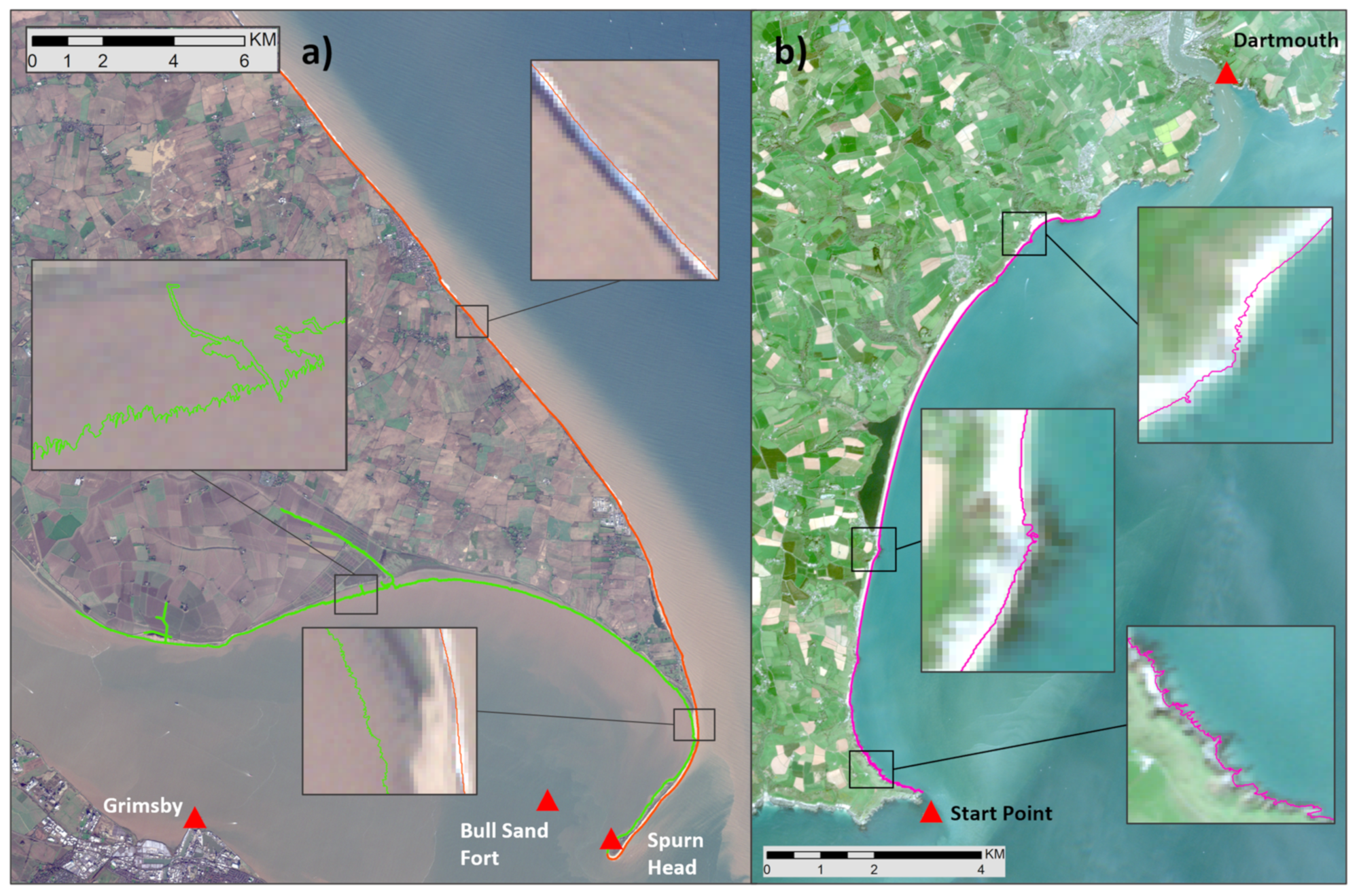
2.1. Study Zones

We have selected two different coastal areas in the UK which cover three different coastal macro-tidal environments: soft cliff open coast (Site #1), estuarine (Site #2), and gravel barrier beach (Site #3) (see Figure 1).
Sites #1 & #2 are located at Spurn Head on the east coast of England, which forms the southern extremity of the Holderness coast. It consists of a 5.5 km sand, gravel and cobble dynamic coastal spit that extends south-westwards across the mouth of the Humber estuary in shallow water. The Holderness coast extends 61 km from Flamborough in the north to Spurn Point in the South and, at a rate of ca. 2 m per year, is one of Europe’s fastest eroding coasts [16]. It is a macro-tidal soft coast, with a tidal range of up to 7 m [16], subjected to the force of the waves from the North Sea with little attenuation before they reach the cliff line. The seabed consists of glacial mud, sand, and boulders, as do the cliffs (consisting of low superficial deposit cliffs ranging from 3 m to 35 m in height). Spurn Point has evolved and is maintained by coarse sediment supplied from the erosion of the Holderness shoreline [17]. The wave energy is lower inside the Humber estuary, which is a shallow macro-tidal zone with processes driven by the power of the tides. The incoming tidal currents carry more sediment into the estuary than the tides carry out, and its turbidity is due to suspended sediments that come mainly from the eroding Holderness cliffs [18]. The estuary is 14 km across at its widest point and its average depth is 6.5 m. It has been modified by human activities for over 2000 years and it is estimated that half of its intertidal area has been lost due to land reclamationfor agricultural and industrial developments [18].
Site #3 is at Start Bay, a 12 km long embayment located on the south coast of Devon, where the effects of erosion, accretion, and beach rotation have been well-studied and documented [19]. The embayment comprises five sub-embayment gravel barrier beaches, named from the south to north as; Hallsands, Beesands, Slapton Sands, Forest Cove, and Blackpool Sands. Between each sub-embayment lie short headlands/rocky outcrops. Within Start Bay, gravel is finer to the east due to the lateral grading of material [20], with coarser grains transported southwest with larger, easterly waves, and finer grains being well sorted and transported northeast with smaller, but more frequent, southerly swells. The tidal range can reach up to 6 m and the wave climate in Start Bay is modulated by Start Point, a rocky headland offering shelter from longer period southerly waves, and Skerries Bank, an offshore banner bank that sits east of the main beaches in the southern half of the embayment and is −5 m Ordnance Datum Newlyn (ODN) at its shallowest. Furthermore, the entirety of Start Bay is bound by large headlands, and the system is considered a closed sediment cell, with no sediment sources except for some confined areas of cliff erosion [19].

2.2. Historical Shorelines Database from MSI and SAR Imagery

Table 1 summarizes all of the EO products that we have used for this study. These have been produced as part of the European Space Agency funded “Coastal Change from Space” project [10]. Lead by ARGANS Ltd., this project brought together professional geomorphological expertise from partners at the British Geological Survey (BGS), the Geological Survey Ireland (GSI), the Environmental Hydraulic Institute Cantabria, and Arctus, working with the University of Quebec, Rimouski (UQAR) as part of a Coastal Change consortium. The project focused on conducting assessments over 25 years using a range of satellite sensors such as Copernicus Sentinel MSI and SAR data in addition to USGS Landsat data, supported with a blend of some commercial data provided by the ESA Third Party Mission program.
The MSI and SAR imagery dataset used combines data from Sentinel-2 (S2) and Sentinel-1 (S1) missions. The different product types used for this study are: (1) waterlines (WL) which are a proxy tideline (a physical feature taken to represent the coastline) extracted from all missions (S1, S2) and (2) shorelines (SL) which are derived from the waterlines where the location has been corrected to take into consideration the beach profile and adjusting to a tidal level, to produce a shoreline-corresponding user-defined given tidal level or Datum.

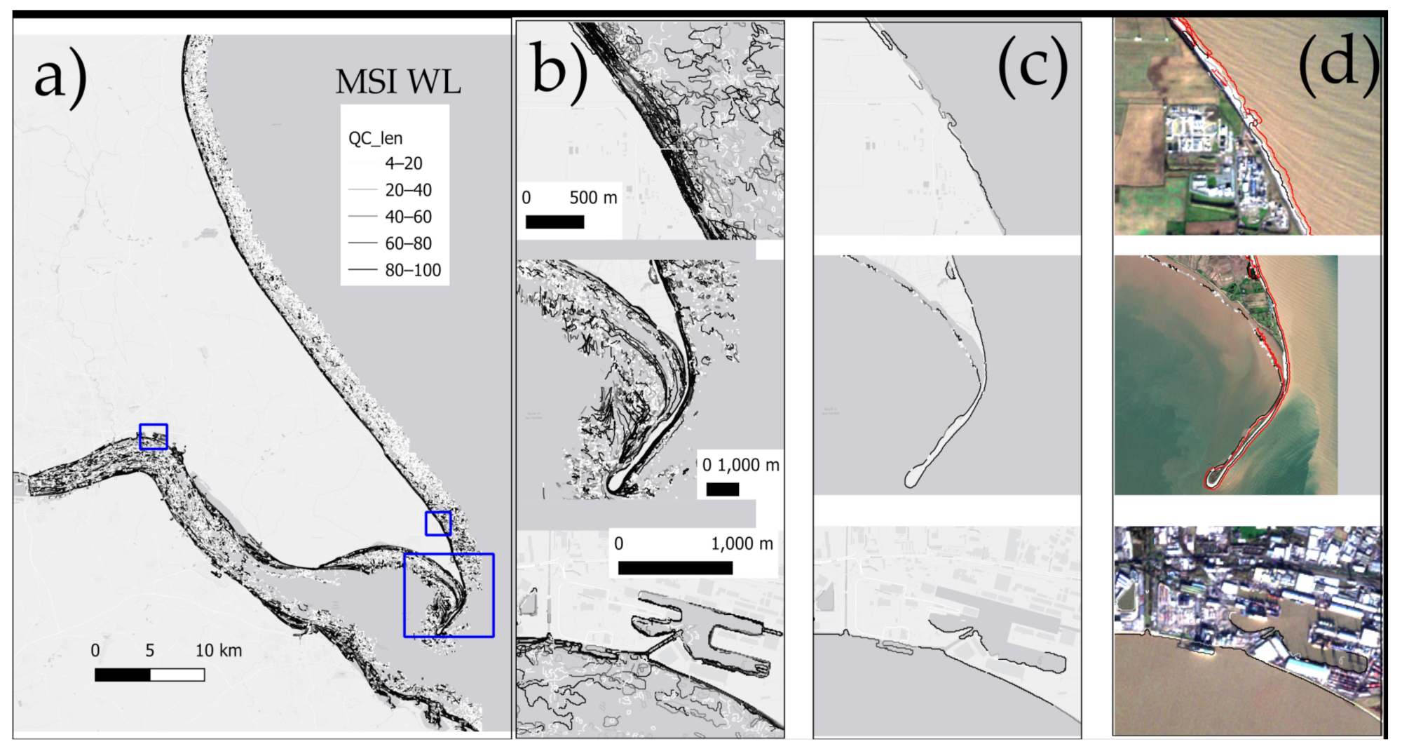
2.2.1. Process Used to Delineate the Historical WL and SL from Publicly Available Satellite MSI Imagery

Very High Resolution (VHR) commercial satellite images were used to correct pixel offsets, or co-register, to improve the spatial accuracy of both WL and SL obtained from the MSI imagery. This processor provides multiple shoreline proxies computed from optical observations from Landsat 5/8 and Sentinel-2 missions without considering the corrections due to the tidal level at the time when the satellite image was taken, or the slope of the coast. For this study we have used Sentinel-2 mission data only. The WL are then converted into SL at different user defined tidal levels (Mean Sea Level (MSL), Lowest Astronomical Tide (LAT), Highest Astronomical Tide (HAT), Mean Low Water Springs (MLWS) and Mean High Water Springs (MHWS)) (Figure 2). These three processes are briefly explained below, and the reader is referred to [11] for further details.
The co-registration process aims to improve the spatial accuracy of satellite observation. Spatial accuracy is a measure of the location conformity between the different Earth observation pixels and their true location on the Earth surface. From one satellite acquisition to another, the observations are not perfectly overlapping. EO have their own errors and uncertainties that lead to different positioning. The shift can reach up to 12 m for Sentinel-2 [11] and Landsat 8 [21] acquisitions. The adopted co-registration process uses VHR commercial imagery as the ground “truth” and all optical observations are corrected using the open source Automated and Robust Open-Source Image Co-Registration Software (AROSICS) [22]. The software applies a Fourier shift to get the precise X and Y offset at a geographical position.
Once images are spatially corrected, the waterline processor extracts (for each image) the land/sea boundary, producing a waterline that represents the instantaneous water level at the time the satellite passed over the area. For the extraction of the land/water boundary we have used a normalized spectral index combining either blue, red, green, and the NIR band to optimize the spectral distance between water pixels and land pixels. The delineation process relies on a local adaptive threshold applied on the chosen spectral index for the coastal area allowing a precise identification of the land-water boundary. Due to tidal regimes, satellite revisit times and coastal geomorphologies, each waterline is based upon the coastal morphology at the time of satellite passing. All waterlines are attributed with a quality control (QC) score between 0 and 100 created for each waterline segment combing two quality indicators. The QC_len indicator qualifies waterline segment length and calculates the line geometry length. Long continuous waterline segments have higher quality flag number and flag very small waterline segments often detected due to breaking waves or landside bodies of water; these are some of the most common processing errors encountered. QC_LCI measures how compact the segment is relative to its length using a Line Confinement Index (LCI).
L C I = X m a x X m i n + Y m a x X m i n L
LCI shows good ability to isolate the majority of small errors and provide high QC score to short accurate waterline segments. However, this method struggles with complex coastal geometries such as rocky headlands, harbors, groins, and river outlets.
QC_intern blend the two indicators scores and ensures that drawbacks from each method are mitigated. This allows for more accurate flagging of both accurate and erroneous waterline segments. QC_intern is the mean value between QC_len and QC_LCI.
To enable inter-comparison and time-series analysis to indicate movement or change, waterlines are then corrected to a referenced tidal datum height by a stage called the shoreline processing. This process considers various ocean and morphological parameters such as wave height, tidal height, and beach profile to transform a waterline into a shoreline. For each waterline we obtain a set of shorelines at specific datum heights, Mean Sea Level (MSL), for this study. Despite consistent results in production supported by in situ validation [23], the shoreline processor has various limitations which must be identified and accounted for. Some of these limitations are inherent and result from input data inaccuracies and, more specifically, the quality and the spatial range of auxiliary data, i.e., the tidal and slope data mentioned above.

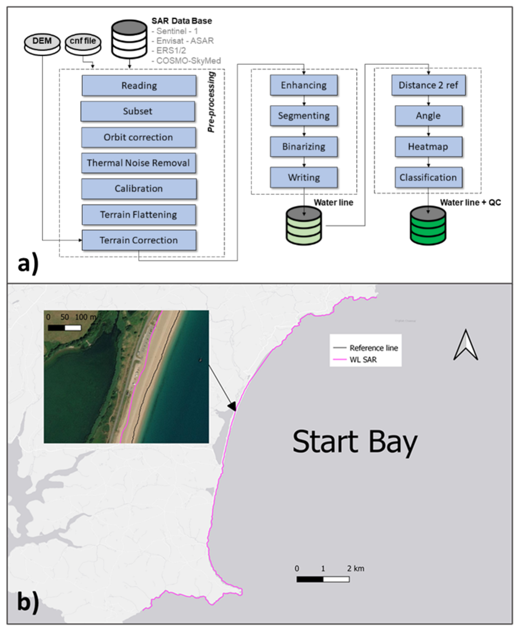
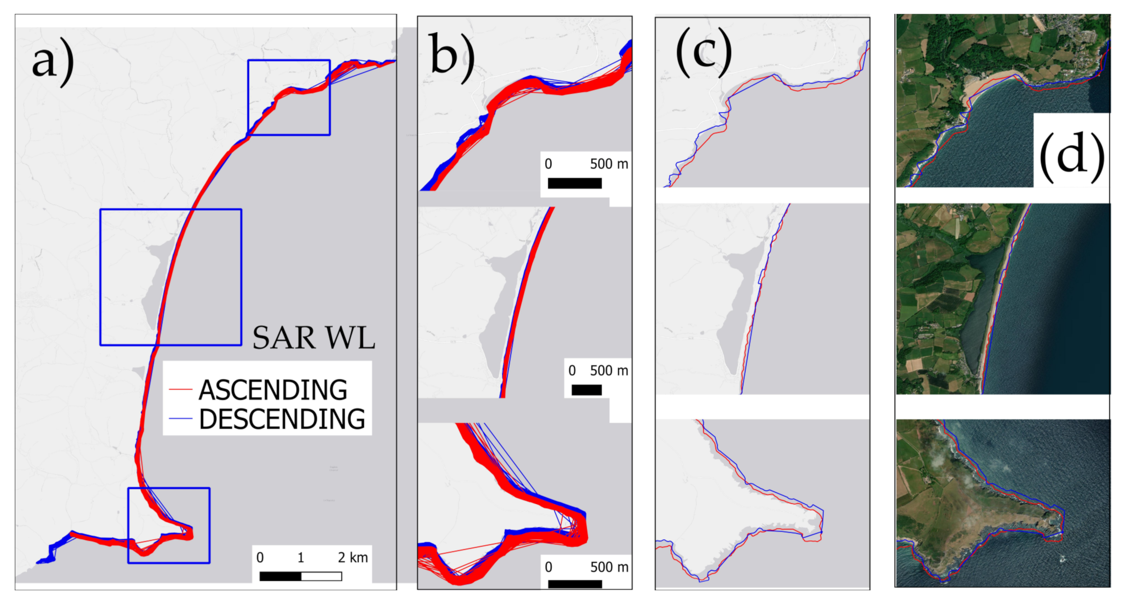
2.2.2. Process Used to Delineate the Historical WL from Publicly Available SAR Imagery

The processing chain consists of three main processes (Figure 3) [12]. In the first process the pre-processing is applied to the SAR data to produce a georeferenced image. The second process is composed by enhancement, segmentation, healing, and vectorization which are defined below. Each of these implement a range of options and are configurable by a range of parameters which can be specified in an input configuration file. The output is a vector line and metadata associated with the image acquisition and the processing configuration used. In the third process the quality control is applied to classify the points of the WL, filtering out the bad results. We have used the vertical transmit and horizontal receive (VH) polarization to extract waterlines from SAR.
In the first stage, SAR data are pre-processed to geo-reference the intensity image in accordance with the WGS84 reference system. This stage is composed by the sub-steps shown in Figure 3 and using the methods already developed within the SNAP tool [24]. After the intensity image is geo-referenced, we proceed with the application of the image processing steps. In order to improve the results of the binary segmentation, the SAR image needs to be enhanced in order to compensate for expected characteristics of the SAR image such as salt-and-pepper thermal noise and illumination gradients caused by antenna beam roll-off. The methods used to enhance the image are based on the Lee and Sigma filters [25] and anisotropic diffusion [26]. The segmentation step produces an initial estimation of the land-sea boundary in the form of a binary raster. This is produced by a simple threshold of the enhanced SAR image. The appropriate intensity value of the threshold is computed using the method from [27]. Once the initial estimation of the waterline has been computed, the binary raster that has been produced is then improved by applying a range of binary morphology operations known as healing [28]. The purpose of this process is to eliminate erroneous features that might appear in the initial estimation of the waterline.
Finally, the third block process is executed in order to compute the three different quality control parameters for the corresponding waterline: the distance to the reference line, angle between the coast, and the satellite ground track and the density of lines. The density indicates the percentage of points, from different temporal measurements, that are close to the current point for the line being evaluated. The distance to the reference is computed against a reference provided at the mean tidal point for each of the points from the SAR waterline. It can be used in further analysis to measure the evolution of the shorelines and compute trends. The distance and the density are used together to discard outliers (waterlines from artifacts that appear far from the reference line and have a high-density value).

2.3. WL and SL Qualitative Quality Assessment

The aim of the quality assessment described here is not only to assess the quality of the products in terms of their shape and length but also to better understand what shoreline proxy, if any, the WL and SL derived from both MSI and SAR imagery actually represents. Accordingly to [3] these proxies could be (a) a feature that is visibly discernible in coastal imagery, (b) features that are not necessarily visible to the human eye or (c) the intersection of a tidal datum with the coastal profile. The qualitative assessment focuses on assessing which proxy, a or b, EO represents while the quantitative assessment focuses on assessing c.
The qualitative assessment of WL and SL was done in three steps. In particular, for Site #1 & #2 we have analyzed only MSI-WL and MSI-SL derived from Sentinel-2 and for Site #3 we have analyzed all (e.g., MSI-WL, MSI-SL from Sentinel-2 and SAR-WL from Sentinel-1) Firstly, the satellite-derived WL and SL were individually visualized at different scales. This allowed the overall characteristics of the line to be assessed, including its completeness, the presence of any spurious lines, loops, or gaps. The lines were then visualized over the co-registered satellite imagery from which the line has been delineated, allowing an assessment of where they were accurately capturing the coastline and where there were issues. Finally, WL and SL were then compared to Ordnance Survey (OS) tide line data and to other waterlines from different dates to understand if the satellite waterlines were able to detect changes in coastline resulting from erosion. In particular we used OS High Water and Low Water Mark lines from 2015 and 2019 (open data, OS VectorMap District dataset). VectorMap is an open-source dataset, updated twice per year (May and November) and covers Great Britain with a representative fraction scale of 1:15,000 to 1:30,000.

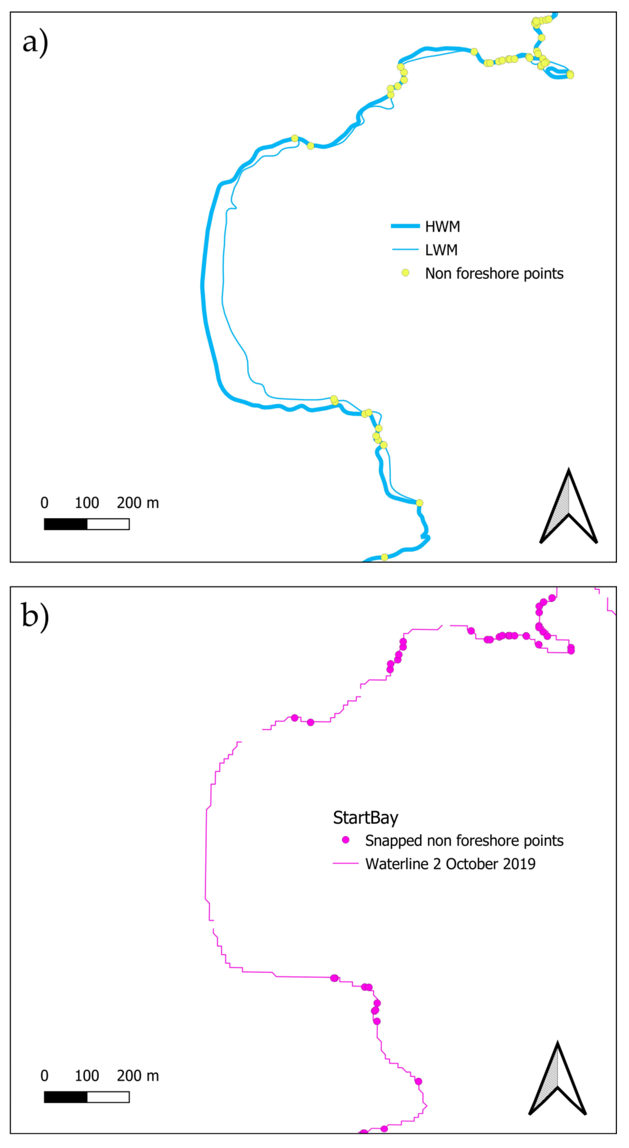
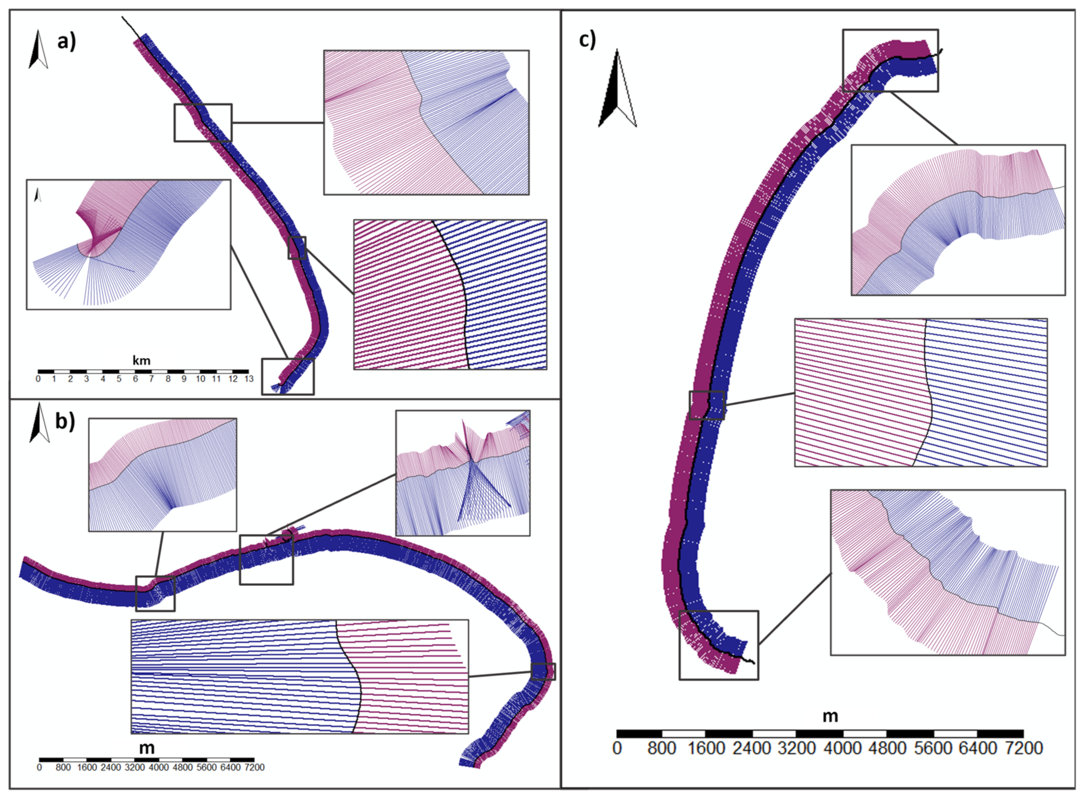
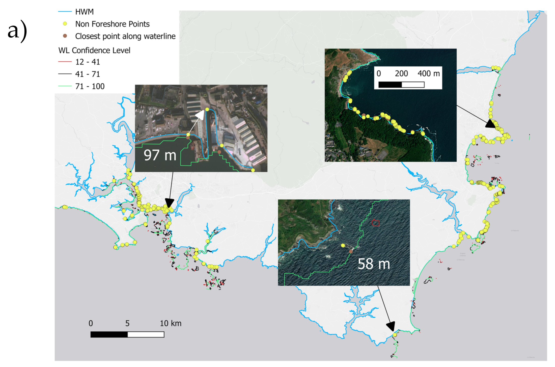
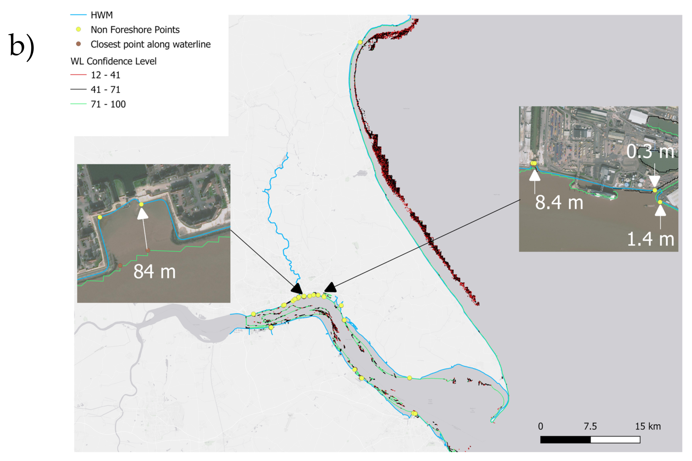
2.4. WL and SL Quantitative Quality Assessment: New Non Foreshore Method

For the quantitative assessment we acknowledge that there is currently no standard method to assess absolute and relative accuracy of satellite-derived waterlines and shorelines. In this context we propose a new method, referred to as the no-foreshore method, to assess the accuracy of these products. For the sake of transparency and reproducibility, all processing is done using the System for Automated Geoscientific Analyses (SAGA) software v8.0.1 which is a Free Open Source Software Geographical Information System (GIS) developed by SAGA User Group Association, Hamburg, Germany [14].
Figure 4 illustrates the key concepts and process followed for the non-foreshore accuracy assessment used in this work. To minimize the uncertainty associated with the water level differences between the time that the satellite image was taken and the ground truth data, we have chosen to focus on locations where there is no foreshore. The foreshore is the area exposed between high and low tide. At locations with no foreshore, the waterline will have minimum variations and its position can confidently be compared to both waterlines and shorelines. The non-foreshore locations were extracted from the intersection of the High Water Mark (HWM) and Low Water Mark (LWM) tidal boundary lines from the OS VectorMap District dataset. For each waterline, we have extracted the closest points to the “no foreshore” points and measured the absolute and relative distances. The absolute accuracy was obtained by taking the distance between a “no foreshore” point and the corresponding nearest point on the waterline using the SAGA-GIS “Point to Line Distance” tool. The relative accuracy was obtained by measuring the distance between two “no foreshore” points and the distance between the corresponding points on the 1D product being assessed. The search of points for the relative accuracy was limited to a circular area with a radius of 500 m, to be consistent with the OS definition of relative accuracy standards. Relative accuracy is normally expressed as a constant plus an amount proportional to the distance measured at different percentages (99%, 95%) of confidence level and Root Mean Square Error (RMSE) value constrained to a maximum distance (which for maps at a fractional scale of 1:10,000 is 500 m).

2.5. Digital Elevation Model Used for Ground Truth Validation: SurfZone 2019

For the ground truth validation of the different products, we have used the 2019 SurfZone DEM produced by the UK Environment Agency and published through the DEFRA Data Services Portal [29] (Figure 5).
The SurfZone DEM model combines LiDAR and near-shore multibeam SONAR bathymetry elevation data. It is the best currently available DEM covering the inter-tidal zone. The SurfZone DEM was produced using a bespoke feathering technique to smooth the overlaps between LiDAR and bathymetric surveys to produce a seamless surface. Where small gaps existed between both surveys, these were interpolated using a bilinear interpolation technique. DEMs were downloaded as a tiled raster dataset in GeoTiff format. Each tile is 5 × 5 km and aligned to the Ordnance Survey National Grid. Each pixel represents 2 m spatial resolution on the ground and elevations are presented in meters to Ordnance Survey Great Britain (OSGB) using the OSGM’15 and OSTM’15 transformation models. Elevations are referenced to Ordnance Datum Newlyn. The data is also available as an ESRI Image Service enabling use of the data at source with GIS. Errors in elevation DEM values are of the order of ±0.5 m. The tile corresponding to Start Bay was mapped between 19th and 21st April 2019 and the one from Spurn Head was mapped between 26th and 27th November 2019. The WL products available and closest in time to the date at which the DEM was collected are the ones produced from the MSI images taken on 3 December 2019 at 11:13 UTM for Spurn Head and 20 April 2019 at 11:21 UTM for Start Bay.

2.6. Method Used to Compare with Ground Truth and Calculate Metrics of Coastline Change

We have used Transect and Baseline Analysis (TBA) [30] to both compare the WL products with datum-based ground truth tidelines and to calculate the different metrics of coastline change. The TBA is based on the measurement and comparison of the distance between each shoreline at set points along transects. We have used the ODSAS [13] method that allows explicit inclusion of the resolution of the study as part of the process via a Digital Elevation Model (DEM) that is then used to delineate the transects. The first part uses SAGA-CliffMetrics [31] for transect generation and SAGA-ProfileCrossings [13] to obtain the shoreline distances along each transect. The second part uses R environment and CoastCR [13] to obtain the main metrics of coastline change.
We have used theCliffMetrics software tool [31] to (1) delineate the datum tideline (referred to here as ground truth) from a DEM that is then compared with the WL and (2) generate the transects to user-defined baseline. CliffMetrics uses a wall-follower algorithm to delineate the coastline along the DEM that best fits the requested elevation [31]. The resulting user defined datum-based coastline is both a raster and vector point coastline. The raster coastline layer represents the raster cell in the DEM whose elevation at each cell is the closest value to the user defined elevation. The vector point coastline represents a smoothed line where the smoothing is defined by the user. The delineated transects are located perpendicular to the vector coastline, extending to the seaward-side or landward-side (e.g., controlled by the user with the sea handiness parameter) from each raster coastline cell for a user-defined transect length. The correct level of smoothing is decided by the user on an iterative, manual process of transect delineation and visualisation.
The baseline used in the TBA approach is derived from the non-smoothed, datum-based tideline extracted from the SurfZoneDEM using CliffMetrics. Figure 6 shows the baselines on top of the Sentinel-2 images whose time of collection corresponds most closely to the time that the SurfZone DEM data were collected at each site. The astronomical tidal elevation at the time the satellite images were taken has been obtained from POLTIPS3 v3.9.0/16 coastal tidal software [32]. POLTIPS-3 is an easy-to-use software package for Microsoft Windows that is used to compute the tides at coastal locations around the UK. The software, developed by the National Oceanographic Centre, uses the most powerful tidal computation engine available, which is used by the UK Environment Agency to compute tidal levels. Figure 6 shows the tide gauge stations available in POLTIPS3 for the two study sites. All astronomical tide levels are referred to Ordnance Datum Newlyn which is the same datum used for the DEM. We have used the astronomical tidal elevation at Spurn Point for the Spurn Head Site, which was 1.64 m at the time the satellite image was taken. At the Start Bay Site, we used two tide gauges: Start Point and Dartmouth, which at the time the satellite image was taken had elevations of −1.30 m and −1.17 m, respectively. Using both elevations, we compared the lines extracted using CliffMetrics, without smoothing, and noticed that the horizontal differences between the two datum-based tidelines were of the order of 1 m with no clear spatial bias. We decided to use the astronomical sea level value at Start Point because it is an open coast location and is less likely to be influenced by the local bathymetry than the value at Dartmouth, which is located with anestuary.
Figure 7 shows the baseline and transects used for this study. An equal number of transects at the sea-side and land-side of the baseline are created at a constant interval to enable a comparison between shorelines. The datum-based tideline extracted from theSurfZone DEM with no smoothing is jagged as it follows the raster cells and needs smoothing to avoid the transects changing direction sharply. To ensure that transects do not change orientation sharply we have used CliffMetrics again but now, using the vector datum-based tideline extracted from SurfZone, iteratively tried different smoothing options until we were satisfied with the transect orientation. To ensure that transects were generated every 10 m the baselines shapes were converted to points separated by 10 m for the three sites; 2604 transect were generated for Sites #1 & #2 with a coastline smoothing algorithm running mean window size of 20 and 1302 transects were generated for Site #3 with a smoothing running mean window size of 25.
CoastCR is an algorithm programmed in R that filters out the intersections between baseline transects and the historical shorelines and calculates the main metrics of change summarized in Table 2. These parameters capture both absolute horizontal coastline change (values in m) and annual change rates (values in m/year). Absolute horizontal coastline changes are easier to process than change rate ones (LRR and WLR and their associated errors). For the change rate parameters, the CoastCR routines generate several loops to calculate all parameters and take longer. NSM and EPR rates are the simpler parameters to obtain. NSM is the difference between the youngest and the oldest coastlines, and EPR is the NSM divided by the timespan in years. The SCE calculates the maximum variation between all coastlines along all transects. LRR rate is the average rate of change for all transects, where for each transect the rate of change is calculated as the slope of the line resulting from a least-squares regression line. Finally, the WLR is similar to LRR but uses the associated uncertainty of each shoreline to estimate the best-fit line. In this case, the weight was estimated as a function of the variance in the uncertainty. The outputs obtained after running the method are the statistical parameters listed in Table 2 for each transect (as a shapefile containing all the transect lines) and aggregated for all transects as a table report with the Mean, Standard Deviation, Maximum, Median, Minimum values (see Appendix A for more details).
To perform the PCA we used the MATLAB R2021b (The Mathworks, Inc., Natick, MA, USA) “pca” function, specifying the Singular Value Decomposition algorithm, without centering the data and using all data after the NaN values were removed (e.g., no interpolation of missing data). The original dataset is a matrix containing the filtered distances along each transect, obtained using the ODSAS approach, organized in N columns and M rows representing the number of transects and shoreline dates, respectively. We first removed the columns (dates) with NaN values and then the rows. The resulting size of the dataset used has the following N × M sizes: 2491 × 36 for Spurn Head and MSI shoreline database, 964 × 37 for Start Bay MSI shoreline dataset, 1117 × 379 for Start Bay SAR descending orbits, and 1117 × 387 for Start Bay SAR ascending orbits.

3. Results

3.1. Qualitative Assessment

We present here the qualitative assessment of MSI-WL and SL, and SAR-WL for the different study sites and EO missions.
Figure 8 shows MSI WL from Sentinel 2 analyzed for Site #1 & #2. A visual inspection of MSI WL indicated that the WL were predominantly continuous with few spurious lines. Some gaps were present, but these did not appear to be too detrimental to the understanding of the line as a first iteration. When the lines are plotted in a grey scale (Figure 8a) using one of the quality control indicators (QC_len) (with low-quality score in grey and high-quality score in black) the low-quality line segments appear to be mostly in the nearshore and low intertidal areas. A zoomed view at different regions (Figure 8b) also revealed that the water lines are not mapped, as expected, in the cliff backshore. The resolution of the image and delineation algorithm is able to detect the small lagoon in the backshore, the narrow neck of the spit of ca. 120 m and the sharp edges of the docking areas within the harbor including the narrow 25 m harbor entrance channel. It was observed that the number of spurious segments and the ability to detect the narrow harbor entrance channel is sensitive to the tidal level at the time that the satellite image was taken. For example, Figure 8c shows a waterline extracted near high water level resulting in minimum spurious lines and also the harbour channel not being detected. The location of the waterline, extracted when the tidal level was close to high water, relative to the shoreline at MSL is as expected in the open coast (e.g., SL-MSL is seaward than WL). There is no SL-MSL in the estuarine area because the intertidal slope was not provided to correct the WL.
Similar results are found for Site #3 as shown by the analyzed MSI WL from Sentinel-2 shown in Figure 9. The delineation algorithm is able to detect the very irregular rocky platform outcrops. Some gaps were present, but these did not appear to be too detrimental to the understanding of the line as a first iteration. The location of the waterline, extracted when the tidal level was close to low water, relative to the shoreline at MSL is as expected in the open coast (e.g., SL-MSL is landward than WL). There is no SL-MSL in the southern rocky outcrops area because the intertidal slope was not provided to correct the WL.
Figure 10 shows the SAR WL from Sentinel-1 analyzed for Site #3. A visual inspection of SAR WL indicated that the WL were predominately continuous with no spurious lines. Figure 10a shows the WL extracted from images taken during Ascending and Descending orbits for the entire study area. In places, the WL appears as spurious rectilinear segments most appreciable at the northern and southern ends of the large embayment. A zoomed view at different regions (Figure 10b) showing at all lines in bulk revealed that there is not a clear tendency of lines extracted from one orbit to appear systematically landward or seaward to the other. Figure 10c shows two WLs extracted near high tide two days apart which confirms that there is not a clear bias between WL extracted from images taken at different orbits, but instead ascending and descending lines appear relative to each other in landward and seaward locations. SAR WL seems able to delineate both the relatively homogeneous and rectilinear gravel beach and the very irregular rocky outcrops.

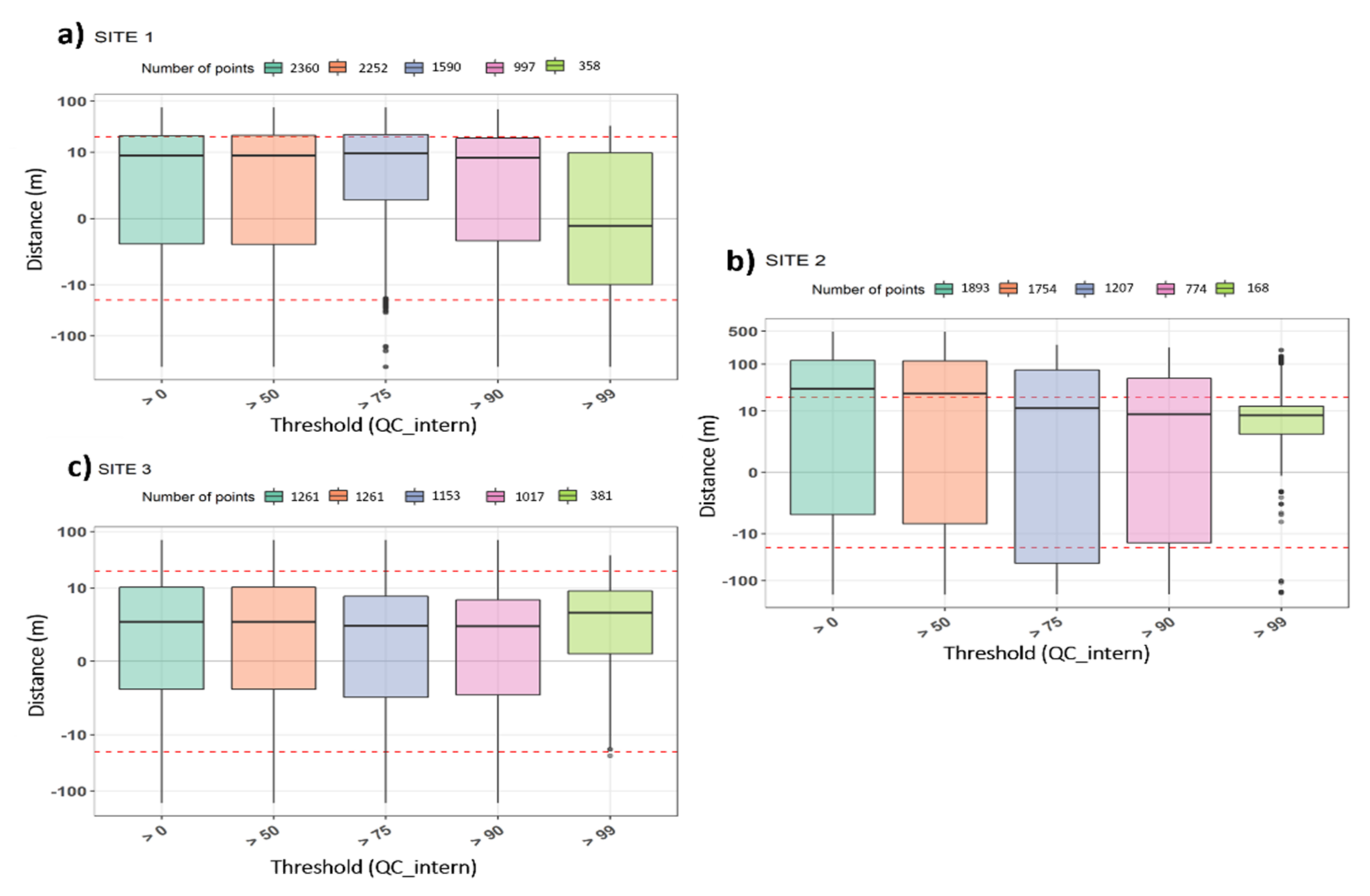
3.2. Quantitative Assessment

Figure 11 shows the results of applying the non-foreshore method to calculate the absolute and relative accuracy of MSI-WL produced from S2 at all study sites. We have used the S2 MSI images dated 11:06:31 UTC 25 June 2020 at Site #1 & #2 and 11:21:21 UTC 2 October 2019 at Site #3. The number of non-foreshore points used to assess the absolute accuracy are 74 for Sites #1–2 and 1449 for Site #3. The number of non-foreshore point-pairs used to assess the relative accuracy is 68356 for Sites #1–2 and 354 for Site #3. The lower number of non-foreshore points at Sites #1–2 is due to the gentler intertidal slope at these sites relative to the steeper intertidal slope at Site #3. The few non-foreshore points are located near built-up areas (i.e., harbors and levees) where the WLs are not always continuous. The absolute and relative RMSE values for Site #3 are 19.7 m and 14.2 m, lower than the values obtained at Site #1–2 which were 41.6 m and 23.0 m, respectively. The histograms of the distances between the non-foreshore points and the closest point on the MSI-WL have a gaussian shape suggesting that there is a significant bias on the position accuracy at Site #3 but not at Sites #1–2 (see Figure A1). To better understand the non-normal distribution at Sites #1–2, Figure 11e shows the points used for the non-foreshore approach to quantify the MSI-WL accuracy. For the limited number of non-foreshore points at Sites #1–2, where the WL is continuous, the absolute error varies from 8.4 m to 0.3 m and comparable with representative fractions from 1:600 to 1:16,800. The representative fraction has been calculated here as 0.5 mm/RMSE [33]. At Site #3, the accuracies are equivalent to representative fractions from 1:24,800 to 1:51,400 which are comparable with the representative fraction scale for OS VectorMap District of 1:15,000 to 1:30,000. These RMSE and representative fraction scales should be considered as a conservative estimate of the resolution of the MSI-WL resolution, as we have used all segments without filtering out the segments flagged as poor quality.
Using the datum-based tideline extracted from the SurfZone DEMand one S2-WL at each study site we have calculated the differences in both elevation and shoreline position. The differences in the horizontal position has been calculated using the baseline-transects method, with the datum-based tideline as baseline, and the elevation differences from the elevation values extracted from the SurfZone DEM along the datum-based tideline and WL. To facilitate the interpretation of the graphical results presented here we have indicated in the figures a representative error, ±ε, where ε is defined here differently for horizontal and elevation difference plots. For location or horizontal distances, ε is defined astwofold the length of the diagonal of the pixel size of the satellite image used, which for S2 is 10 m resolution resulting in ε = 2 × (102 + 102)1/2 = 28 m. For the elevation differences, ε is defined by the SurfZone DEM vertical accuracy ε = ± 0.5 m.
Figure 12 shows the elevation and position differences between the datum-based tideline and the S2-WL. A visual inspection of the location of the datum-based tideline and S2-WL (Figure 12a,b) revealed that the greatest differences are in the estuarine area (Site #2) and the smallest along the gravel beach at Site #3. This is confirmed by the numerical values shown as violin plots in Figure 12c. These illustrate the horizontal distances between the datum-based tideline and each S2-WL, with positive and negative values indicating that S2-WL is located seaward and landward to the datum-based tideline respectively. The percentage of values that fall within the representative error for position differences is 85%, 50%, and 90% for Sites #1, #2, and #3 respectively. The median value of position differences for all three sites is positive, suggesting that S2-WL tend to be on the seaward side of the datum-based tideline. This seaward bias of S2-WL is also reflected in the lower elevation values (e.g., negative elevation differences in Figure 12d) when compared with the elevation of the datum-based tideline. The percentage of values that fall within the representative error for elevation differences is 50%, 90%, and 72% for Sites #1, #2, and #3 respectively. For Site #3 there were parts of WL that were outside of the DEM, so the vertical distances studied were not the elevations corresponding to the whole line, but only a segment of it. Some of the elevation differences between the datum-based tideline and the S2-WL might be due to the uncertainty derived from how the datum-based tideline has been extracted from the DEM. To quantify this uncertainty, we have plotted (Figure 12e) the distribution of the differences between the elevations extracted from the DEM along the datum-based tideline and the datum value used (1.64 m for Spurn head and −1.3 m for Start Bay). We found that the differences are the order of the vertical accuracy of the DEM. Table 3 shows the numerical values of the main statistical parameters represented in the violin plots in Figure 12.
Figure 13 show the horizontal position accuracy varies when only a subset of the MSI-WL segments is used and Table 4 shows the corresponding median values. The subset is obtained by filtering MSI-WL segments with a minimum threshold value of the quality score, QC_intern, of 0, 50, 75, 90, and 99. The differences in the number of points for the different threshold score values are the order of hundreds of points. For example, the number of points that have a threshold value equal or larger than 99 were three times less than the points over the 90 threshold and six times less than the total points analyzed. Results at each study site are different but in general it seems that threshold values of 50 & 75 suffice to ensure that position accuracy is within the representative error ε. The use of highest threshold values (90/99) results in a significant reduction of the number of points to compare in the subset without significantly improving the accuracy. At Site #1, regardless of the threshold value used, the accuracy values are always within the representative error; with the bigger appreciable change appearing when using a threshold score value higher than 99, where the median accuracy reduces from 7.7 m to just −0.3 m. At Site #2, we found that a threshold score value larger than 50 is needed to ensure that the median accuracy value is within the representative error. Additionally, using a threshold score value of 99 reduces the number of points drastically but keeps some outlier points outside the error range. At Site #3, accuracy value is always within the representative error range and the use of different thresholds does not produce relevant changes or a clear trend. We noticed that there are points with the best quality score (100) that have larger differences with the datum-based tideline position than points with lower scores.

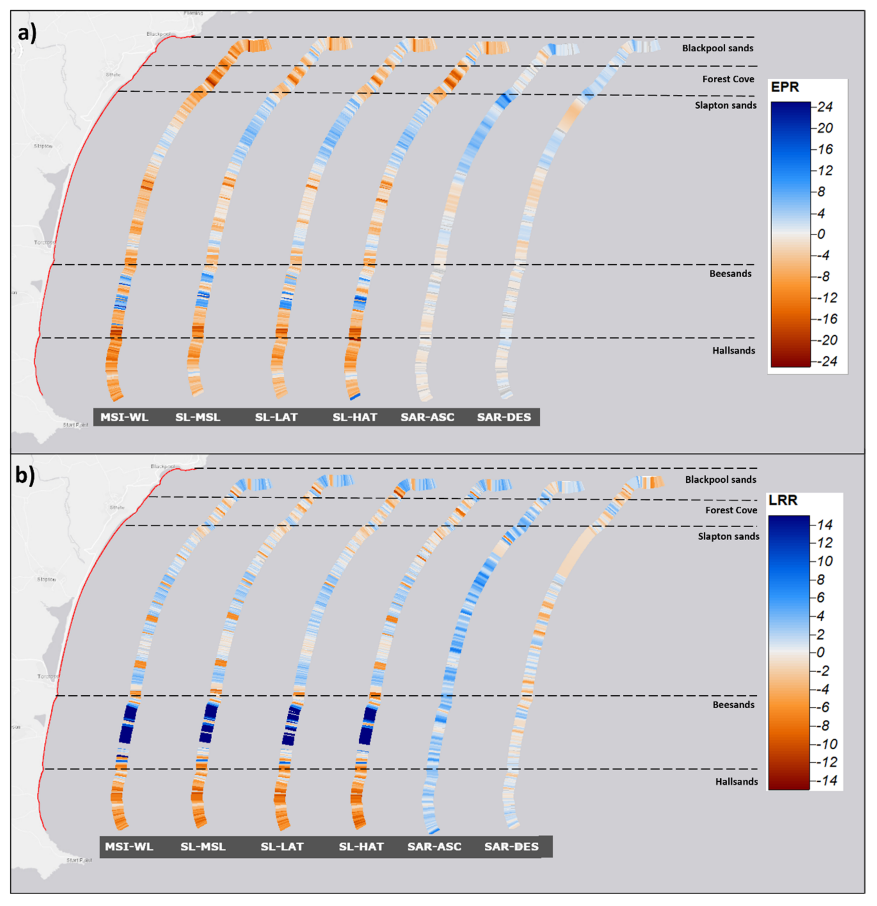
3.3. Coastline Annual Rate Change Results Using Both MSI WL, SL and SAR Products

Table 5 shows, for all transects, the aggregated values of the NSM, SCE, EPR, and LRR for Site #3 using different MSI and SAR lines for the period 2016–2019. We have used 1177 transects from the 1302 that were generated for Site #3 shown in Figure 7. We have also expressed the mean and standard deviation (SD) values for each parameter as non-dimensional ratios relative to the values obtained using the MSI-WL. There are gaps in the MSI lines that results in some transects not intersecting some lines and not having values of distances for those dates. These values are necessary to calculate some of the rates so there are transects for which the rates were not obtained. Table 5 also shows the percentage of the 1177 transects that were used for each annual rate calculation. SAR lines do not have any gaps and we were able to calculate the rates for all transects. For this study period, and according to the MSI-WL, the two parameters that represent the scale of change, NSM and SCE, are of the order of 10 m with an SD of the same order. The NSM and SCE values are consistently smaller by a factor between 0.5 to 0.9 relative to the values using SL derived from MSI-WL. The NSM values derived from SAR-WLs are significantly different between Ascending and Descending orbits and to the one obtained using MSI lines; bigger than the values for MSI-WLs by a factor of 1.3 for SAR-ASC lines and reduced by a factor of −0.3 for SAR-DES lines. The SCE values derived from SAR-WLs are quite similar by a factor of 0.9 to 1 to the MSI lines, with differences smaller than 12 m. The EPR and LRR are global parameters that represent annual change rate (m/year) and are of the order of 10 m for the study period and sites. MSI shoreline results for EPR differ from MSI-WL with variations of the same order as for NSM, being consistently smaller. The bigger differences were found for EPR values with SAR lines in which SAR-DES show erosion and SAR-ASC lines show accretion. Values of LRR obtained for MSI-WL show erosion, with smaller values for the datum-based SL changing by a factor of 0.3 and 0.5. In contrast to MSI lines results, SAR lines show small accretion in the LRR rates, with similar values of the order of 1 m for both types of lines: ascending or descending.
Figure 14 represents EPR and LRR annual rates for each of the 1177 transects at Start Bay. The individual transect values for EPR varies from a minimum of −23 m/year to a maximum of 99 m/year and from −13.8 to 15.7 m/year for LRR. EPR values from datum-based MSI lines and MSL-WL are similar along the beach, with significant accretion in two sections; one at the northern end of Beesands beach and the other at the southern end of Slapton Sands, with a rocky coast separating both sections. All MSI lines show high values of erosion at the south of the study area. Values of EPR and LRR derived from SL-MSL and MSI-WL are very similar. We observed higher differences with SL-LAT, which for example is not showing the same small erosion zone in the middle of Start Bay that we can see in the rest of the MSI results. SL-HAT shows higher erosion values than SL-MSL and SL-LAT in the northern part of Forest Cove but in better agreement with MSI-WL results. EPR and LRR values from SAR lines display considerate disparity between them (e.g., suggesting orbit dependence) and differences to MSI lines. SAR-ASC change rate results suggest that accretion dominates while SAR-DES suggest that erosion dominates. Values of EPR for SAR are smaller than values derived from MSI-WLs and positive for SAR-ASC and mostly negative and close to zero for SAR-DES. LRR results for different MSI lines show similar changes in the same areas, but there are bigger differences with the values obtained for SAR lines. Both SAR lines have small values of LRR closer to 0 m/year and they do not show the accretion observed in MSI results. Discrepancies between them appear at the north in Forest Cove area where SAR-ASC rates have accretion values and SAR-DES rates slightly tend to erosion. Although the EPR and LRR aggregated values shown in Table 5 suggest that the annual rates of SAR-ASC lines are of a similar order of magnitude to values obtained from MSI-WL, the individual transect values do differ significantly. To assess the influence of the location uncertainty of each individual MSI-WL in the WLR values, we have used the absolute accuracy values from the quantitative assessment (RMSE = 19.7 m), obtaining a mean WLR value of −3.1 m/year with a standard deviation of −3.6 m/year, which represents a reduction of a factor of 0.9 of the mean value of LRR obtained for the same lines.
Table 6 shows the aggregated values of NSM, SCE, EPR, and LRR calculated with 30 MSI-WLs for Site #1 for the time period from December 2017 to June 2020. Values of NSM and SCE represent a scale of change of the order of 100 s of meters with a SD of the same order. Transects used for NSM are 24% less than for SCE due to line gaps. The mean values of EPR and LRR, using less than 90% of the transects available, is of the order of −30 s m/year with extreme values (maximum and minimum) of the order of 100 s/m.
Figure 15 shows the spatial distribution of the EPR and LRR annual rates calculated using MSI-WL and SL-MSL at Site #1 between 2016 and 2019. Table 6 shows the numerical values of the main metrics of change aggregated for all transects (N = 2604). EPR values were calculated using 76% of the total transects because of the gaps that appear in initial and final MSI-WLs used. LRR values are less affected by the gaps and were calculated using 89% of the transects available. A visual inspection of the spatial distribution of the EPR values suggest that, where there are transect by transect differences, there are no large differences in the overall pattern (e.g., clusters of erosive and prograding transects in similar environments) when using WL or MSL historical lines. The aggregated values do confirm the overall similarities with EPR values of similar order (−13 and −15 m/year) using WL and SL-MSL, respectively. The largest differences are on the SD of the EPR values, which are by a factor of 0.8 smaller the SD derived from SL-MSL. Conversely, there is a significant difference between the LRR values both at transect by transect level and aggregated level with LRR mean values being a factor of 2.3 larger and of the order of −23 m/year when using SL-MSL than when using the WL without the tidal correction.

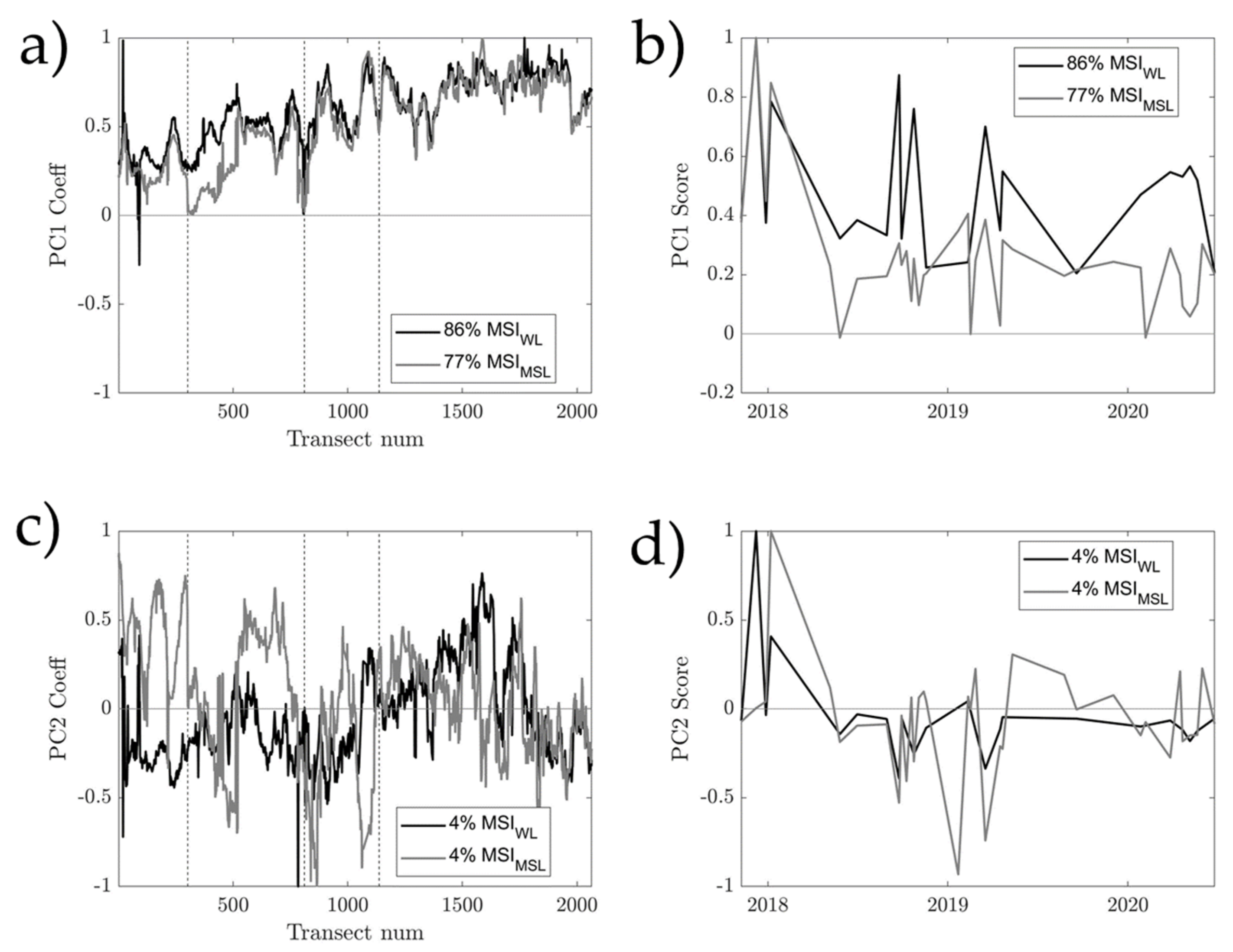
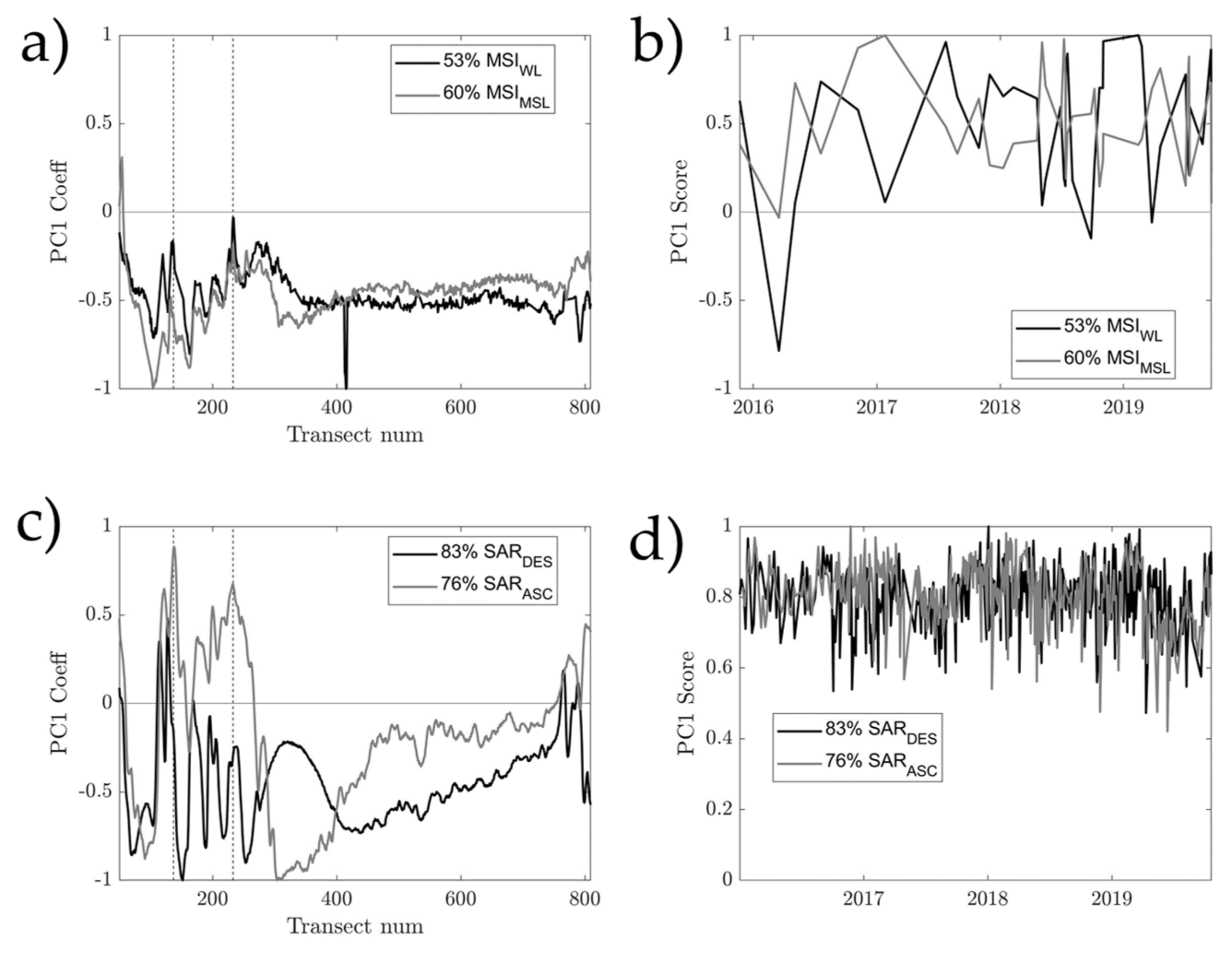
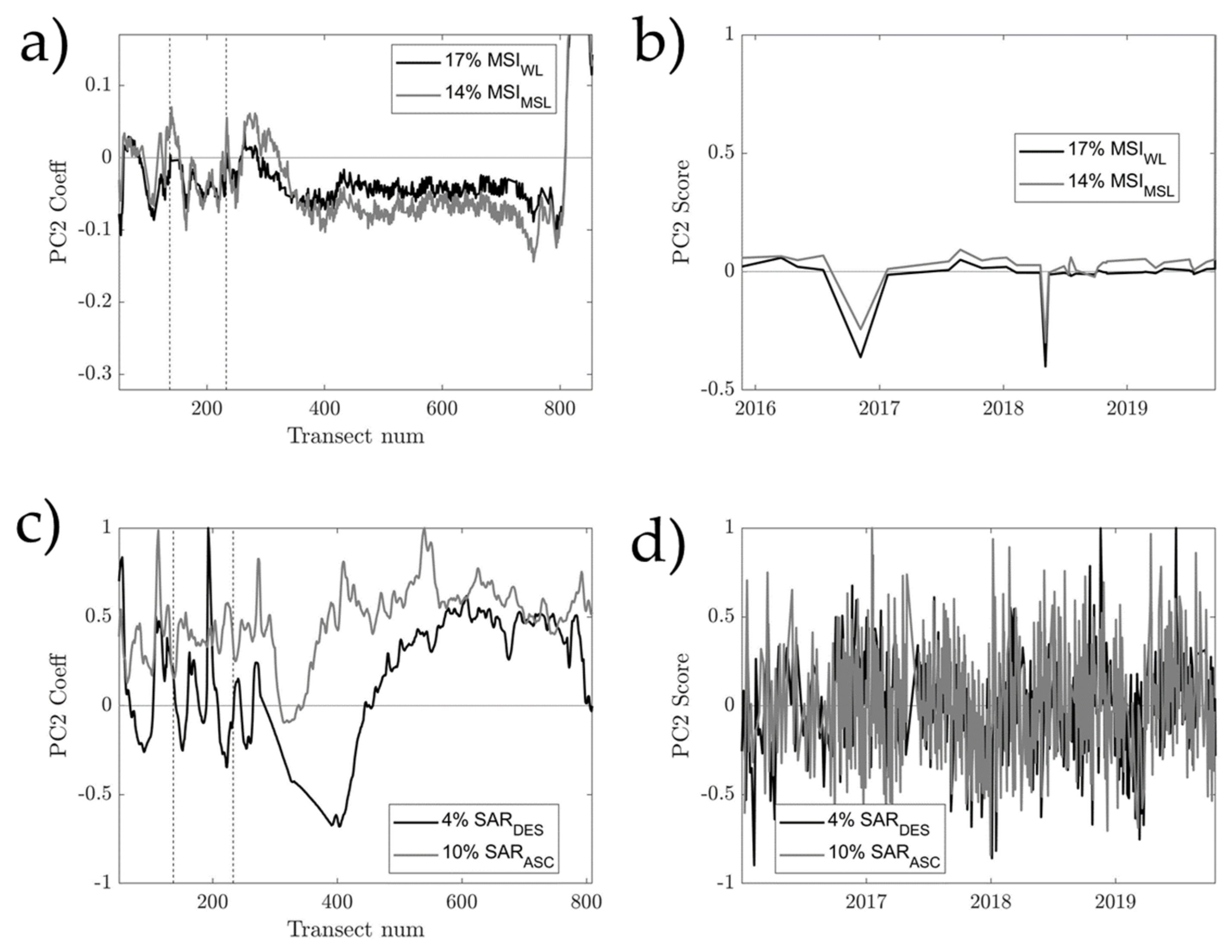
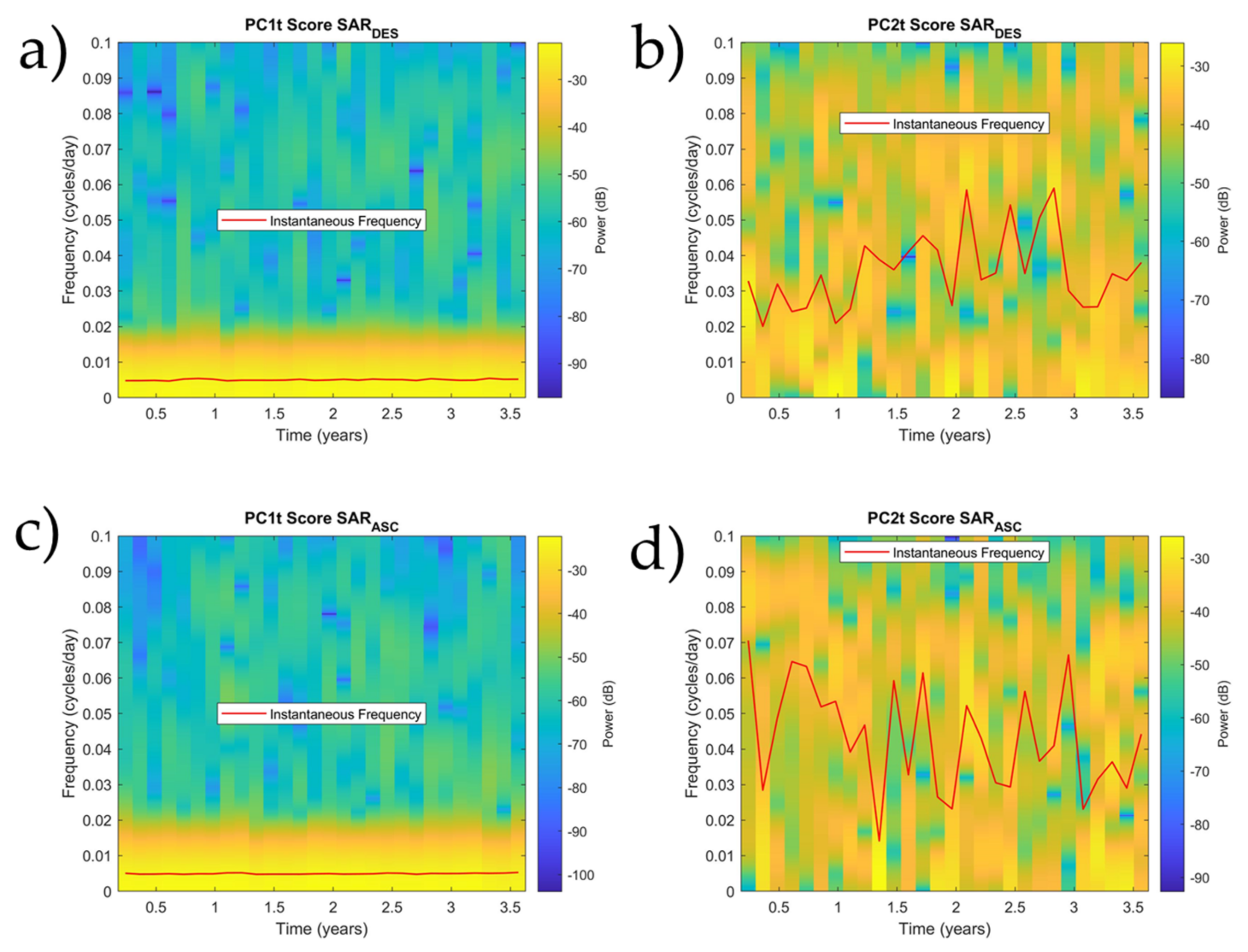
3.4. Extraction Shoreline Variability via Empirical Orthogonal Function Analysis

We have extracted the first two principal components (PC1 and PC2) for the MSI and SAR shoreline databases at study sites #1 and #3 using the relative shoreline position derived from each alongshore location (transect) and for each time step [9]. Figure 16 shows the location and transect ordinal numbers that we have used to facilitate the interpretation of the spatial variability of the PCA scores at each study site.
Figure 17 shows the PC1 & PC2 coefficient and scores for the Spurn Head area using the MSI WL and MSI MSL shoreline databases which together account for 90% and 81% of the total variability respectively. The PC1 coefficients spatial variability derived from both WL (e.g., affected by tidal levels at the time of the observation) and MSL are very similar between the Beacon Ponds (#811) and Whithernsea (#2064) and slightly different between Spurn Head (#1) and Beacon Ponds. Most of the PC1 coefficient values are positive with the exception of nodes (e.g., coeff. values close to zero) near the Gas terminal (#1137) and Beacon Ponds and a local minimum with negative values between transects #1 and #302. Spatial coefficients without nodes are more reflective of the typical shoreline response to cross-shore processes where the entire coastline advances or retreats in phase [9]. The differences between WL and MSL temporal scores are more significant throughout the study period with the MSL temporal mode suggesting a decrease in early 2018 followed by a more stationary period after mid 2018, with up to four events for which a node in the temporal score was reached. The PC2 coefficients of spatial variability, which only represents 4% of the total variability, illustrate different alongshore spatial patterns resulting from WL and MSL shorelines. The results derived from WL indicate a local absolute maximum near the Beacon Ponds (coeff. ca. −1) and a local maximum (coeff. values ca. 0.6) between the Gas terminal and Whithernsea. The results derived from MSL indicates an absolute maximum near Beacon Ponds, with large coeff. values (ca. 0.5) close to Spurn Head. The presence in both datasets (WL & MSL) of a number of zero crossings or pivot points suggest that this variability is controlled by longshore sediment transport. These pivots points are nodal points that typically separate adjacent areas of erosion and accretion (coefficient change sign) and therefore shoreline changes are often referred to as being out of phase across a node. The PC2 temporal scores are for most of the study period close to zero with no clear trend.
Figure 18 shows the first principal component (PC1) coefficients and scores for the Start Bay area using the MSI WL & MSL, and SAR ASC & DES shoreline databases. The percentage of variability explained for both SAR DES and ASC lines is 83% and 76% respectively and greater than the MSI WL & MSL which is 53% and 60% respectively. Most of the PC1 coefficient values for the MSI lines are negative and around −0.5 value with the exception values for MSL near the northern end of Blackpool Sands (#50). It is noted that at the headland locations of Blackpool Sands and Forest Cove (#50, #137, #233) the values are close to zero suggesting that they are nodes or points of minimum shoreline change. This is expected behavior of steep rocky outcrops with limited or no foreshore. The locations of maximum variability, with values close to −1 are between transects #413 to #416 (e.g., the area where the road was damaged during the 2018 storm event as shown in Figure 18a) for WL and near the center of Blackpool Sands (#104) for MSL. The coefficient values of PC1 for the SAR DES and ASC lines are similar for Blackpool Sands showing positive values around the headlands (#50 & #137) and negative values of ca. −0.7 between the headlands. For the other embayments (Forest Cove and Slapton), PC1 coefficients for SAR DES and ASC are significantly different suggesting that the variance of the two lines dataset might be due to different processes and not only shoreline change. The temporal scores for PC1 derived from MSI and SAR datasets are mostly positive but with significant differences in variability. Scores from MSI shows greater variability over time, with three events during which scores values changed from positive to negative. Scores from SAR are always positive and oscillate around 0.8.
Figure 19 shows the second principal component (PC2) coefficients and scores for the Start Bay area using the MSI WL & MSL, and SAR ASC & DES shoreline databases. The percentage of variability explained for both SAR DES and ASC lines is 4% and 10% respectively and smaller than for the MSI WL & MSL which is 17% and 14% respectively. Most of the PC2 coefficient values for the MSI lines are negative and around −0.05 with the exception of values for MSL near the northern end of each of the three embayments (Blackpool Sands#50, Forest Cove #137 and Slapton #233) where values are close to zero or positive. It is noted that at Blackpool Sands there is a node point around the center of the embayment suggesting a shoreline change in the opposite direction in the northern section relative to the southern one (e.g., as expected when beach rotation occurs). Coefficient values along Forest Cove (#50 to #137) show areas with near zero values that are well aligned with the rocky outcrops and local minimums aligned with the sandy beaches between the outcrops. Along Slapton embayment (#233 to #809) the coefficient values are positive or near zero at the northern end and consistently negative at the southern end (e.g., transect numbers greater than #400). The coefficient values of PC2 for the SAR DES and ASC lines are very different with lines from SAR ASC mostly positive with the exception of a few transects (between #308 and #345) mostly negative. Conversely, PC2 coefficient values from SAR DES shows the alongshore variability that we would expect; nodes at embayment headlands and rocky outcrops and pivot points at expected locations in Blackpool Sands (#67) and Slapton (#457). The temporal scores for PC2 derived from MSI and SAR datasets are on average close to zero but with significant differences in variability. PC1 scores from MSI show smaller variability over time than from SAR with two events (6 November 2016 and 5 May 2018) during which score values changed from positive to negative while scores from SAR oscillate around zero with a frequency of 0.04 cycles per day.
Figure 20 shows the instant frequency estimated from the SAR ASC and DES datasets over the power spectrograms. PC1 temporal mode is dominated by a signal of dominant frequency around 0.005 cycles per day (or 200 days period), while PC2 temporal mode is dominated by a signal of dominant frequency around 0.05 cycles per day (or 20 days period). We found that Start Bay is dominated by semi diurnal harmonics that will result in two cycles per day, but this frequency is not apparent from the analysis of the SAR lines datasets because the sampling frequency of the SAR at this site is at maximum only about one image per day. Therefore, the minimum frequency that can be detected without aliasing is, according to the Nyquist Theorem, ca. 0.5 cycles per day (e.g., half the sampling frequency). The observed dominant frequencies for PC2 scores ar eone order of magnitude smaller than the highest frequency that can be detected and closer to the spring neap cycle which for this area is over a 14.8 day cycle, or 0.068 cycles per day.

4. Discussion

The detailed analysis presented here of MSI and SAR satellite-derived waterlines, obtained from three different macro-tidal environments along the coast of England, UK, indicate that these publicly available data are suitable to map the shoreline location with accuracies (Figure 11 and Figure 12) comparable with the representative fraction scale for OS VectorMap District of 1:15,000 to 1:30,000. The comparative analysis revealed that the horizontal accuracy varies significantly (Table 3) for the three different geomorphic environments included in this study. The median deviation from ground truth data is on the order of 2 m for gravel beach and rocky outcrops (Site #3) and 8 m for gently sloping, estuarine and soft cliff coastal environments (Sites #1–#2). MSI-WL are not always continuous, with gaps and spurious lines often present (Figure 8 and Figure 9). In contrast, lines derived from SAR imagery present no gaps or spurious lines, however their location seems sensitive to both the coastline orientation and the satellite orbit (Figure 10). We have also shown how the error on the overall horizontal accuracy can be slightly mitigated by filtering the MSI-WL segments using a combination of two quality scores used in [11] (Figure 13 and Table 3). The comparison between the datum-based tideline extracted from SurfZone DEM and the MSI-WL at all three sites (Figure 12) revealed that MSI-WL tend to be more often in the seaward (lower) side of the datum-based tideline (Table 3). Similar to the bias between proxy HWL shorelines described by [34], this bias between the satellite-derived waterline and the datum-based coastline will need to be corrected when combining these two types of coastlines on shoreline change analysis.
Our shoreline change analysis was performed using the TBA method and the historical lines derived from MSI satellite indicated that care is needed interpreting the results. At Sites #1 & #3, we have shown how the ERR and LRR values (Figure 14 and Table 5 for Site #3 and Figure 15 and Table 6 for Site #3) obtained using WL and SL derived from a ca. five-year historical database of MSI imagery from Sentinel-2 do differ significantly at both transect-by-transect level and aggregated values. As we have used the same baseline and transects for both WL and the different SL (MSL, HAT, LAT) when calculating the metrics of change, the differences are only attributable to a significant difference between the location of the WL (e.g., non-corrected for tidal level) and the SL (referenced to same datum).
The PCA analysis of historical coastlines, derived from both MSI and SAR satellite images at Sites #1 and #3, suggest that the database contains additional information to the one reported using other data sources to assess coastline change. For example, the changes along the spit at Spurn Head between 2011–2018 reported by [17] are comparable to the ones shown in Figure 15, Figure 16 and Figure 17 for 2016–2019. The spit anchor area is dominated by erosion and the spit head by accretion with a stable point (shown as a node point in Figure 17 at transect #302) at the neck of the spit. We cannot comment on the comparability of erosion rates obtained in our study with the one reported in [17] because the reported area is different. It has been reported that coastline change in this area is a cyclic combination of both cross-shore and alongshore sediment transport processes [35] with our analysis further suggesting that most, approximately 80%, of the variability is dominated by cross-shore movements and less than 4% is dominated by alongshore sediment transport. Start Bay (Site #3) is a well-documented [19,36,37,38] example of embayment beach rotation that occurs at seasonal to inter-annual timescales. During the 2016–2017 period dominated by easterly waves, sub-embayment counter-clockwise beach rotation was observed at Beesands, Slapton Sands and Blackpool Sands [19]. This sub-embayment behavior appears to be captured by PC2 spatial and temporal results from both MSI and SAR images. The spatial PC2 scores for MSI-WL and SAR-DES show nodal points that match the location of the rocky outcrops that separate the sub-embayment (Figure 19). Also, the temporal variability from MSI allows us to narrow down to November 2016 the period when the reported sub-embayment rotation was most likely to occur and even indicates that another similar event might have occurred around May 2018. PC1 scores spatial variability (Figure 18) that seems more related with full embayment rotation (e.g., no nodal points at rocky outcrops) and a larger cyclicity and of the order of 200 days than the 20 days cyclicity observed for PC2 from SAR lines (Figure 20). We acknowledge that more research is needed to better understand the differences between the lines derived from SAR as a function of its orbit and the type and orientation of the coast.

5. Conclusions

The present study contributes to our understanding of a poorly known aspect of using coastlines derived from publicly available MSI and SAR satellite missions. It outlines a quantitative approach to assess their mapping accuracy with a new non-foreshore method. The proposed non-foreshore method takes advantage of locations along the coast where the foreshore is minimum or non-existing. These non-foreshore locations are ideal places to assess the accuracy of the waterlines because its location is minimally affected by water level changes even in macro-tidal environments. The number of non foreshore locations varies with the slope of the nearshore as shown for two of the study sites. For places like Start Bay, with macro-tidal range but steep rocky outcrops along the coast, there are thousands of suitable non foreshore locations on a single Sentinel-2 tile (100 km2). For places like Spurn Head, also macro-tidal but with very gentle tidal flats, the number of non-foreshore points is often limited to places where man-made coastal infrastructure (e.g., harbors, levees, jetties, etc.) exists. This work also illustrates how the resolution of the satellite imagery can be explicitly included when assessing the metrics of shoreline change using the transect and baseline approach. We have used the new Open Digital Shoreline Analysis System (ODSAS) to explicitly include the resolution and provided a guideline with detail step-by-step instructions for anyone interested in using this approach elsewhere. We have also shown how other scales of shoreline change can be extracted using the Principal Component Analysis. This is particularly relevant for SAR-derived waterlines, which potentially contain a richer amount of information on the different scales of change than waterlines derived from MSI imagery for which image usability might be constrained due to cloud coverage. While the challenge of assessing the quality of the extracted waterlines from both MSI and SAR imagery is still in early stages of development, the mapping accuracy and skill in detecting change using publicly available data is comparable to the accuracy of ordnance survey mapping.

Author Contributions

Conceptualization, A.P.; methodology, A.P., M.V.P.-D., A.G.-P., A.-L.B. and S.S.; software, A.P., M.V.P.-D. and A.G.-P.; validation, M.V.P.-D.; formal analysis, M.V.P.-D.; writing—original draft preparation, M.V.P.-D. and A.P.; writing—review and editing, A.P. All authors have read and agreed to the published version of the manuscript.

Funding

This work was financially supported by the Coastal Erosion FromSpace project which was funded via the Science for Society allocation of the 5th Earth Observation Envelope Programme (EOEP-5) of the European Space Agency. M.V.P.-D. stay at the BGS was funded by the International Campus of Excellence in Marine Science (CEIMAR) and co-funded by the UE Erasmus+ Program. AGP was in receipt of an FPU predoctoral contract from the Spanish Ministry of Education and Innovation (reference FPU16/03050) and their stay at the BGS was funded by “Ayudas Complementarias de Movilidad para beneficiarios FPU” from the Spanish Ministry of Education (reference EST19/00682).

Institutional Review Board Statement

Not applicable.

Informed Consent Statement

Not applicable.

Data Availability Statement

The data that support the findings of this study are available on request from the corresponding author, A.P. The data are not publicly available due to third party restrictions.

Acknowledgments

This manuscript was prepared, verified, and approved for publication by the British Geological Survey. We thank the anonymous reviewers for their constructive feedbacks of earlier versions of this manuscript. We would like to thank Olaf Conrad, lead developer of SAGA-GIS, for his support developing the SAGA interfaces for CliffMetrics and ProfileCrossings. Special thanks are also given to the Coastal Change Consortium, a partnership bringing together the delivery of products team, comprising ARGANS Ltd., isardSAT & Adwais EO, and the User Group comprising IH Cantabria, the British Geological Survey, Geological Survey of Ireland and Arctus in collaboration with the University of Quebec at Rimouski.

Conflicts of Interest

The authors declare no conflict of interest.

Abbreviations

The following abbreviations are used in this study:
MSIMulti-Spectral Imagery
SARSynthetic Aperture Radar
ODSASOpen Digital Shoreline Analysis System
LiDARLight Detection and Ranging
ODNOrdnance Datum Newlyn
EOEarth Observation
WLWaterlines
SLShorelines
MSLMean Sea Level
LATLowest Astronomical Tide
HATHighest Astronomical Tide
VHRVery High Resolution
SAGASystem for Automated Geoscientific Analyses
GISGeographical Information System
HWMHigh Water Mark
LWMLow Water Mark
DSASDigital Shoreline Analysis System
DEMDigital Elevation Model
RMSERoot Mean Square Error
NSMNet Shoreline Movement
EPREnd Point Rate
SCEShoreline Change Envelope
LRRLinear Regression Rate
WLRWeighted Linear Regression Rate
SAR_ASCSynthetic Aperture Radar ascending images
SAR-DESSynthetic Aperture Radar descending images
SDStandard deviation

Appendix A

For those readers interested in using ODSAS for similar shoreline change analysis, we provide below step-by-step guidelines. For this guidance we have used a sub-set of the WL available for the Start Bay study area. The software used for these guidelines is SAGA GIS v 8.1.1 (available online: http://www.saga-gis.org (accessed on 20 March 2022)), R-4.1.2 (available online: https://www.r-project.org/ (accessed on 20 March 2022)), RStudio 2021.09.2 Build 382 (available online: https://www.rstudio.com/ (accessed on 20 March 2022)) and CoastCR (available online: https://github.com/alejandro-gomez/CoastCR (accessed on 20 March 2022)).
Table A1. Step by step guidelines to use ODSAS for shoreline change analysis.
Step #DescriptionGraphical Clue
1Load historical coastlines
In SAGA, drag and drop the shapefiles for the historical coastlines. For this example, we have chosen five water lines from S2
Jmse 10 00561 i001
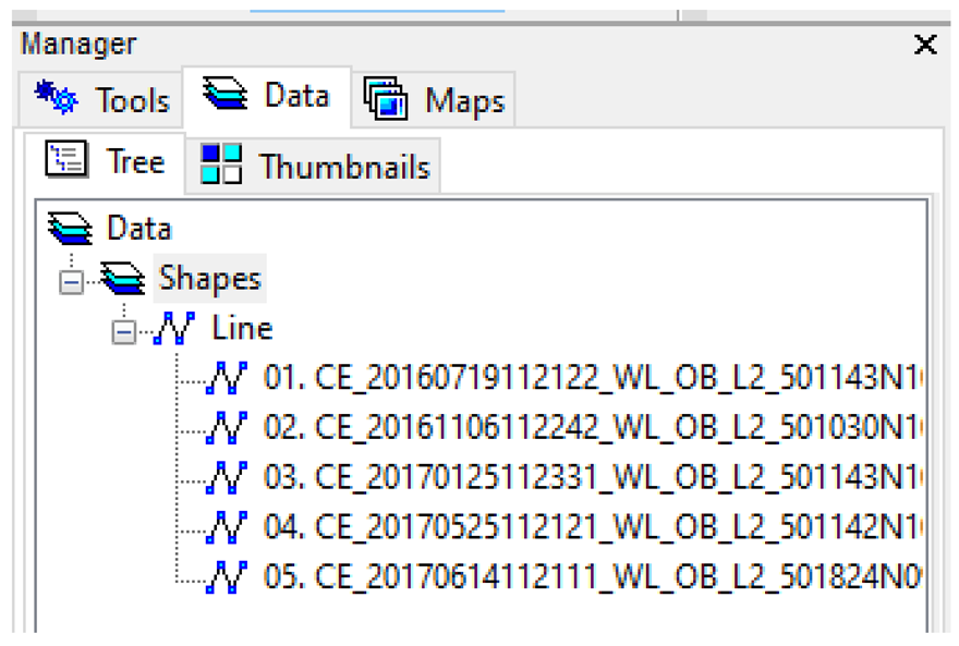
Add DEM to map
Left-click the Data tab and right-click > Add to Map. We have also added Google Satellite as a base map, in the toolbar select MAP > ADD BASE MAP > set Server to Google Satellite
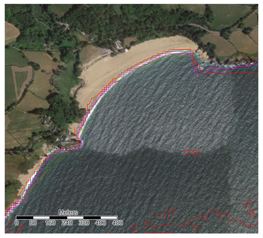
Jmse 10 00561 i002
2Merge all lines into a shape line list.
First, ensure that each date has a single line (e.g., instead of multiple lines). In SAGA, select SHAPES > LINES > LINE
DISSOLVE and set the lines to a historical coastline. Repeat this for all five historical coastlines.
Jmse 10 00561 i003
Secondly, merge all lines in sequential order (e.g., oldest first and more recent last). In SAGA, select SHAPES > TOOLS > MERGE LAYERS and set the layers to the historical DISSOLVED coastlines. Use the Up and Down buttons to sort them in the right order. Jmse 10 00561 i004
Jmse 10 00561 i005
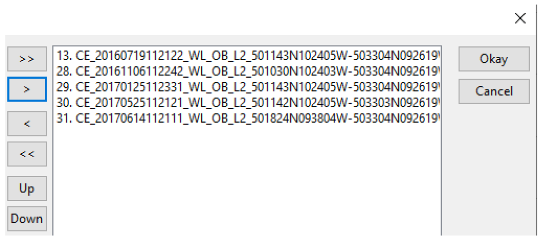
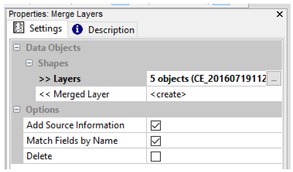
Execute to obtain a Merged Layer with all the historical lines in one file. In our example five lines, the oldest is dated to 19 July 2016 and the more recent, to 14 June 2017. Jmse 10 00561 i006
NOTE: As you will need the date stamp and uncertainty when calculating the metrics of change, save the dates and uncertainty (RMS in meters) as a CSV file (e.g., MyLinesDates.csv) as illustrated on the right.
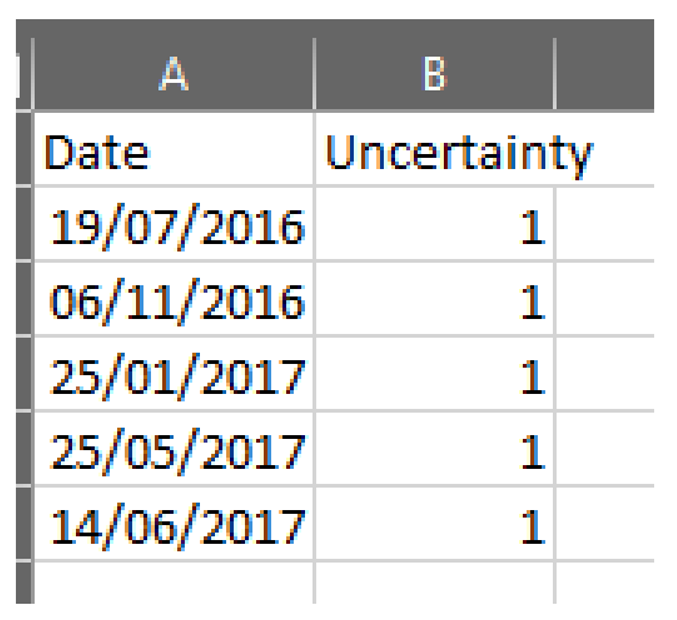
 Jmse 10 00561 i007
3Create shape points Baseline from one of the historical lines
In SAGA, select SHAPES > TOOLS > CREATE NEW SHAPES LAYER > set the options as shown and execute to generate a shape line. Edit the new empty shape line by doing right click, select Edit > Add Shape and start delineating the baseline as you follow your desired reference line. Jmse 10 00561 i008
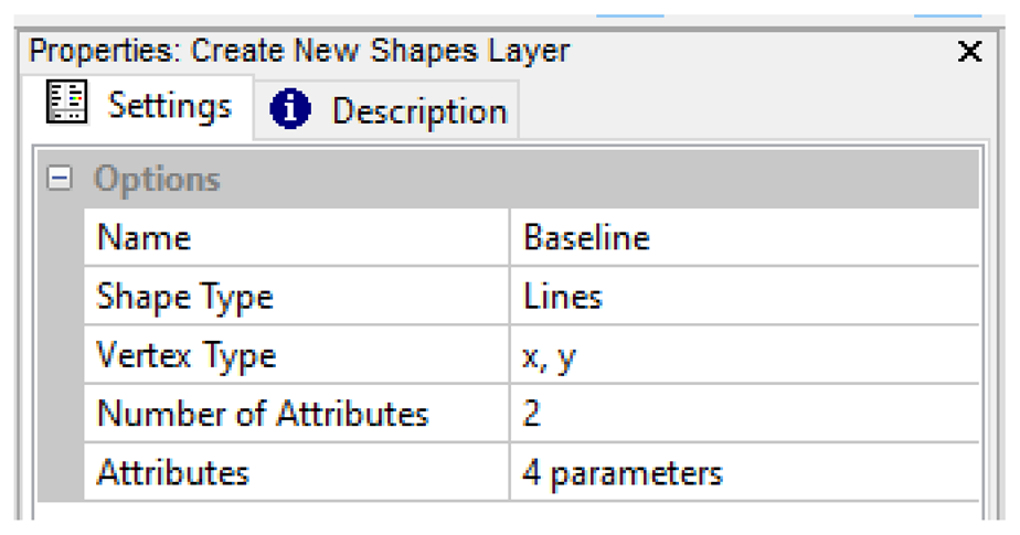
Now convert the shape line into shape points at the user desired distance.
In SAGA, select SHAPES > POINTS > CONVERT LINES TO POINTS > set the Options to Insertion per line and the Insertion Distance (e.g., 15 map units). Execute to generate the shape points baseline. Jmse 10 00561 i009
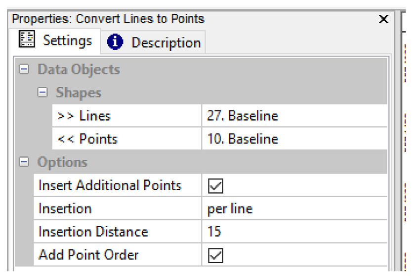
Add to the map to visualize. Red is the historical water line used to delineate the Baseline and green circles are the resulting Baseline.
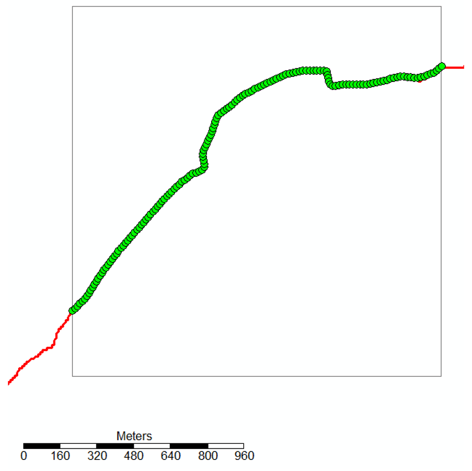
 Jmse 10 00561 i010
4Create a shape polygon of the Area of Interest (AoI)
In Excel, create a table with three columns (ID, X, Y) that represents the X, Y coordinates of the vertex of a rectangle of our AoI > save this as “*.txt TAB separated ASCII” Jmse 10 00561 i011
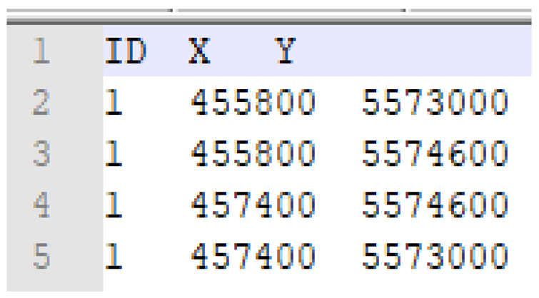
In SAGA, select FILE > TABLE > LOAD TABLE and load the TXT file you just made. Jmse 10 00561 i012
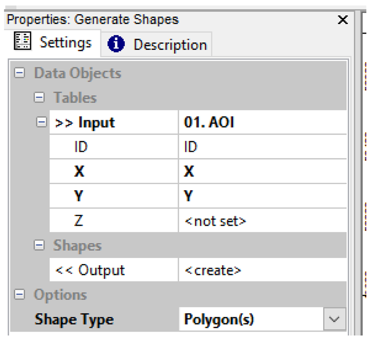
In SAGA, select SHAPES-TOOLS > GENERATE SHAPES and select the AoI table as input, select the fields for X, Y and IDENTIFIER columns and select Shape Type Polygon(s). Click Apply and Execute and you will see a Shapes_AOI Polygon Jmse 10 00561 i013
5Create a dummy grid with the user required pixel resolution.
In SAGA, select GRID > TOOLS >CREATE A GRIDSYSTEM and set the cell size to user-required size (e.g., 10 m) and set the Extent Definition to the AOI shape. Execute to create the dummy grid. Jmse 10 00561 i014
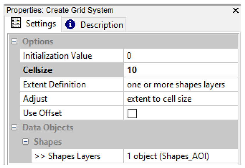
Tip: to visualize the grid cells created, in SAGA select SHAPES > SHAPES-GRID TOOLS > GRID VALUES TO POINTS and set the Grid System to the dummy grid and set the Options Type to cells. Execute to create a shape file points that shows the raster cells of the grid created. Jmse 10 00561 i015
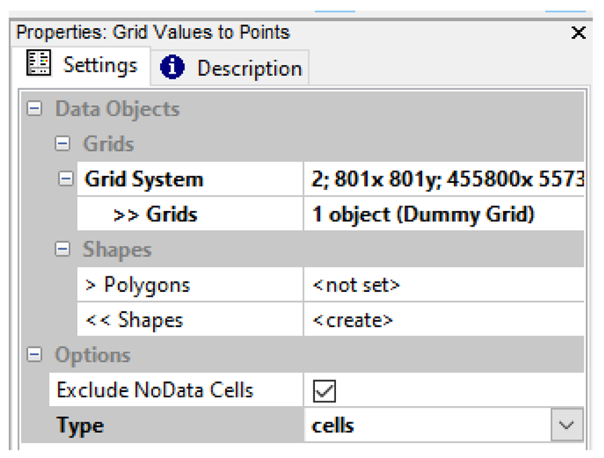
Notice how the Baseline points align with the grid cell in the background.
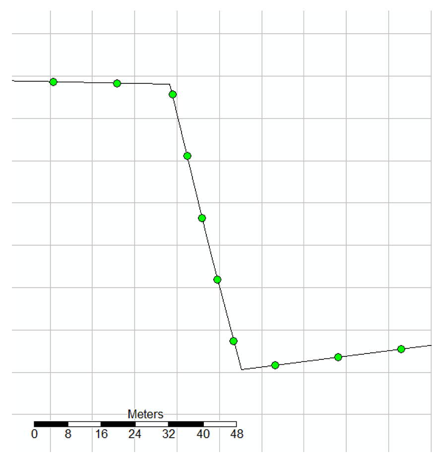
 Jmse 10 00561 i016
6Iteratively create the transects at both landward and seaward sides using different smoothing.
In SAGA, select TERRAIN ANALYSIS > CLIFFMETRICS > CLIFFMETRICS and set the Grid System and Elevation to the dummy Grid. In Shapes, set the User Defined Coastline to the Baseline shape point and the Sea handiness to either right or left and leave the other shapes options unchanged. In the Options select the Coastline Smoothing Algorithm (e.g., running mean, Coastline Smoothing Window 4) and set the Length of Coastline Normals (e.g., 100 m). Jmse 10 00561 i017
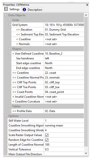
Iteratively play with the different smoothing options until the normal is oriented to your satisfaction and save the normal as either LandwardTransects or SeawardTransects. Repeat the above but changing Sea Handiness to either left or right to obtain the normal for the other side. Jmse 10 00561 i018
NOTE: Be aware that the start of the transects generated by CliffMetrics when tracing the normal is not at the Baseline point location (green circle) but at the centroid of the nearest grid cell (red-black circle) and saved by default as coast_point shape points. Jmse 10 00561 i019
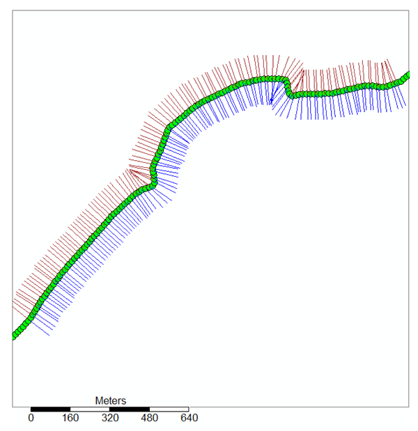
IMPORTANT: the ID number and transects at both landward and seaward side needs to match. This can be checked by confirming that the number of shapes in the Description of both Landward and seaward transects shape lines are the same (e.g., for this example is equal to 136 transects).
To visually ensure that they match we suggest doing the following additional step.
In SAGA, select SHAPES > LINES > LINE CROSSINGS and set the 1st and 2nd Layer to the Landward and Seaward normal that you have just created. Execute and you will obtain a shape point layer with at point at every location where the normal intersects. For most points the intersection will be at the start of the normal (e.g., Landward and Seaward normal share the same start point). Add the crossing points to the map on top of the coast points obtained from CliffMetrics. Delete the normal that does not have a point at the start of the profile.
Jmse 10 00561 i020
Note: the Projection of the Normals is by default the same than for the dummy grid used (e.g., WGS 1984 UTM Zone 30N).
7Calculate distances along transects for all historical coastlines
In SAGA, TERRAIN ANALYSIS > CLIFFMETRICS >COASTAL PROFILE CROSSINGS and set the SeaSide, LandSide and Coast Lines layer as illustrated. Execute to obtain a Shape Point later with all the distances. Distances are positive (blueish) seaward and negative landward (brownish) to the transect start point. Jmse 10 00561 i021
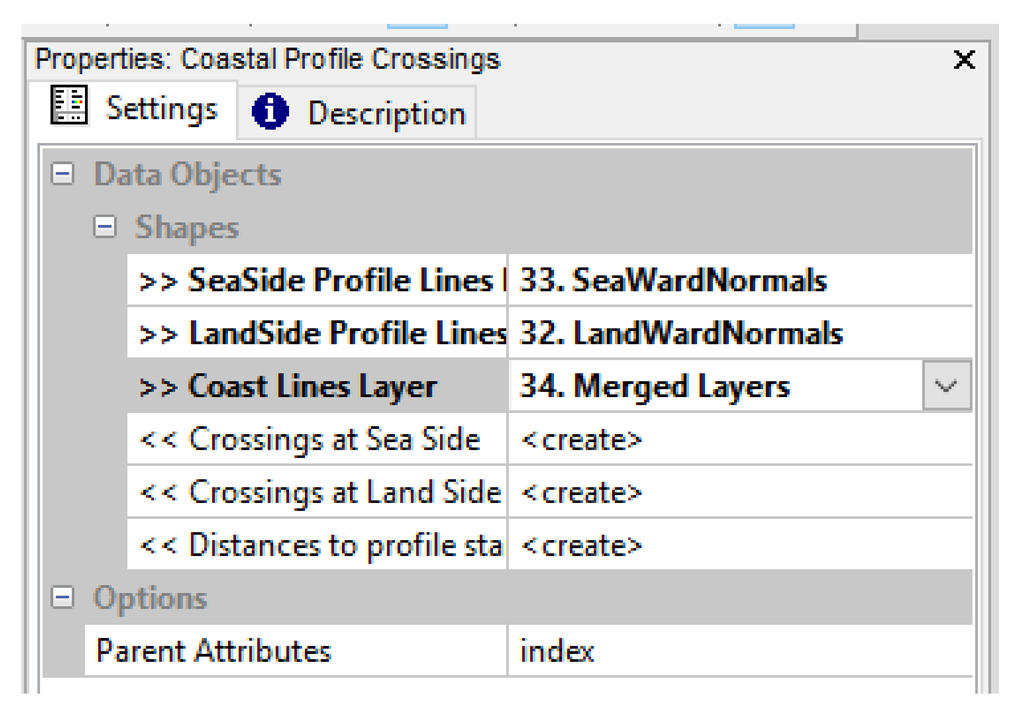
NOTE: notice how in some areas as the one illustrated in the right, there might be lines that are clearly in the water that crosses the transects twice or more. This can be filtered out using CoastCR.
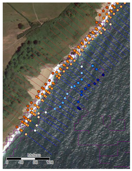
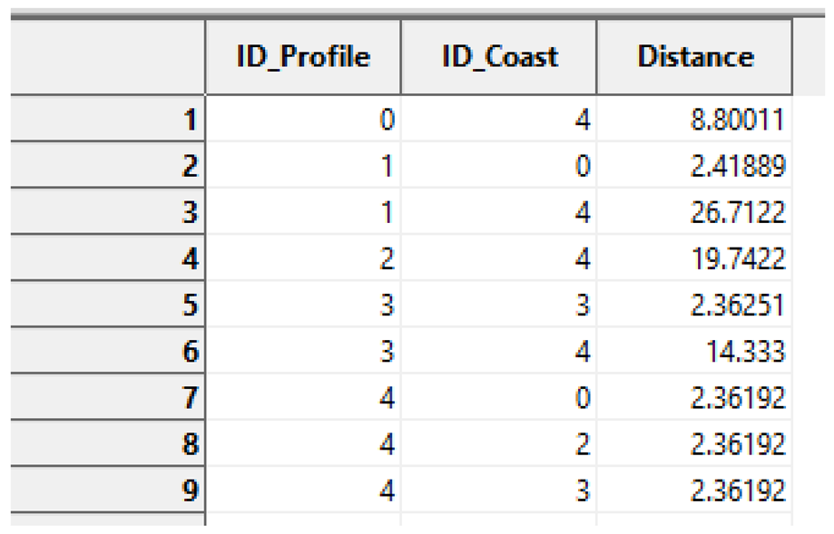
 Jmse 10 00561 i022
Jmse 10 00561 i023
8Calculate the metrics of change using CoastCR
In RStudio, select FILE > NEW FILE > R SCRIPT and copy and paste the code shown in the right panel and run the entire source code by using CTRL + SHIFT +S.
The lines starting with # are just comments to document the code.
#Load libraries
library(sf)
# Install the CoastCR module
remotes::install_github(“alejandro-gomez/CoastCR”)
# Install the CoastCR module
remotes::install_github(“alejandro-gomez/CoastCR”)
# User defined input files
MyCrossingFileName = “…/CrossingDistances.shp”
MyNormalsFileName =“…/SeaWardNormals.shp”
MyDatesFileName = “…/MyLinesDates.csv”
# Baseline position?
# Offshore = OFF; Onshore = ON; Mixed = MIX., position = “MIX”
#User defined Output files
MyFilteredDistancesFile= ”…/DistancesFiltered.shp”
MyErosionStatsFile = “…/MyExampleStats.shp”
# Load user defined input
shp<- st_read(MyCrossingFileName)
normals<- st_read(MyNormalsFileName)
table <- read.csv(MyDatesFileName)
out_points<- MyFilteredDistancesFile
out_name<- MyErosionStatsFile
# Run main program with all inputs
coast_var(shp, normals, table, position, out_points, out_name)
The metric of change aggregated for all transects is saved as a PNG table as the one shown in the right.

The Metrics of change for each individual transect are saved as shape point layer with the user defined output file name (e.g., MyExampleStats.shp)
Jmse 10 00561 i024

Appendix B

This appendix contains additional supporting figures.
Figure A1. Results of the quantitative accuracy absolute and relative assessment at Site #3 (a,b) for waterline extracted from sentinel-2 MSI taken 2 October 2019 at 11:21 UTC and at Site #1 & #2 (c,d) for waterline extracted from sentinel-2 MSI taken 25 June 2020.
Jmse 10 00561 g0a1

References

  1. Mingle, J. IPCC Special Report on the Ocean and Cryosphere in a Changing Climate; 0028-7504; New York Review: New York, NY, USA, 2020. [Google Scholar]
  2. Anfuso, G.; Bowman, D.; Danese, C.; Pranzini, E. Transect based analysis versus area based analysis to quantify shoreline displacement: Spatial resolution issues. Env. Monit Assess 2016, 188, 568. [Google Scholar] [CrossRef]
  3. Boak, E.H.; Turner, I.L. Shoreline Definition and Detection: A Review. J. Coast. Res. 2005, 21, 688–703. [Google Scholar] [CrossRef] [Green Version]
  4. Toure, S.; Diop, O.; Kpalma, K.; Maiga, A.S. Shoreline Detection using Optical Remote Sensing: A Review. ISPRS Int. J. Geo-Inf. 2019, 8, 75. [Google Scholar] [CrossRef] [Green Version]
  5. Luijendijk, A.; Hagenaars, G.; Ranasinghe, R.; Baart, F.; Donchyts, G.; Aarninkhof, S. The State of the World’s Beaches. Sci. Rep. 2018, 8, 6641. [Google Scholar] [CrossRef] [PubMed]
  6. Mentaschi, L.; Vousdoukas, M.I.; Pekel, J.-F.; Voukouvalas, E.; Feyen, L. Global long-term observations of coastal erosion and accretion. Sci. Rep. 2018, 8, 12876. [Google Scholar] [CrossRef] [PubMed] [Green Version]
  7. McAllister, E.; Payo, A.; Novellino, A.; Dolphin, T.; Medina-Lopez, E. Multispectral satellite imagery and machine learning for the extraction of shoreline indicators. Coast. Eng. 2022, 174, 104102. [Google Scholar] [CrossRef]
  8. Vos, K.; Harley, M.D.; Splinter, K.D.; Simmons, J.A.; Turner, I.L. Sub-annual to multi-decadal shoreline variability from publicly available satellite imagery. Coast. Eng. 2019, 150, 160–174. [Google Scholar] [CrossRef]
  9. Miller, J.K.; Dean, R.G. Shoreline variability via empirical orthogonal function analysis: Part I temporal and spatial characteristics. Coast. Eng. 2007, 54, 111–131. [Google Scholar] [CrossRef]
  10. Payo, A.; Hennen, M.; Martinez, J.; Monteys, X.; Jaegler, T.; Martin-Lauzer, F.-R.; Jacobs, C.; Ellis, M.A. Monitoring Coastal Change from space what end users need and what is feasible. In Coastal Management 2019: Joining Forces to Shape Our Future Coasts; ICE Publishing: London, UK, 2020; pp. 213–228. [Google Scholar]
  11. ARGANS. Optical Waterline Algorithm Theoretical Baseline Document. Available online: https://coastalerosion.argans.co.uk/src/SO-TR-ARG-003-055-ATBD-WL-VNIR.pdf (accessed on 11 November 2021).
  12. ARGANS-ISARDSAT. SAR Waterline Algorithm Theoretical Baseline Document. Available online: https://coastalerosion.argans.co.uk/src/SO-TR-ARG-003-055-ATDB-WL-SAR.pdf (accessed on 10 November 2021).
  13. Gómez-Pazo, A.; Payo, A.; Paz-Delgado, M.V.; Delgadillo-Calzadilla, M.A. Open Digital Shoreline Analysis System: ODSAS v1.0. J. Mar. Sci. Eng. 2022, 10, 26. [Google Scholar] [CrossRef]
  14. Conrad, O.; Bechtel, B.; Bock, M.; Dietrich, H.; Fischer, E.; Gerlitz, L.; Wehberg, J.; Wichmann, V.; Böhner, J. System for Automated Geoscientific Analyses (SAGA) v.2.1.4. Geosci. Model Dev. 2015, 8, 1991–2007. [Google Scholar] [CrossRef] [Green Version]
  15. Core Team, R. R: A Language and Environment for Statistical Computing; R Foundation for Statistical Computing: Vienna, Austria, 2013. [Google Scholar]
  16. Sistermans, P.; Nieuwenhuis, O. Holderness Coast (United Kingdom); Eurosion: Amersfoort, The Netherlands, 2013. [Google Scholar]
  17. Bateman, M.D.; McHale, K.; Bayntun, H.J.; Williams, N. Understanding historical coastal spit evolution: A case study from Spurn, East Yorkshire, UK. Earth Surf. Processes Landf. 2020, 45, 3670–3686. [Google Scholar] [CrossRef]
  18. Partnership, H.N. About the Humber Estuary. Available online: http://www.humbernature.co.uk/estuary/ (accessed on 10 November 2021).
  19. Wiggins, M.; Scott, T.; Masselink, G.; Russell, P.; McCarroll, R.J. Coastal embayment rotation: Response to extreme events and climate control, using full embayment surveys. Geomorphology 2019, 327, 385–403. [Google Scholar] [CrossRef]
  20. Chadwick, A.J.; Karunarathna, H.; Gehreis, W.R.; Massey, A.C.; O’Brien, D.; Dales, D. A new analysis of the Slapton barrier beach system, UK. Proc. Inst. Civ. Eng. Marit. Eng. 2005, 158, 147–161. [Google Scholar] [CrossRef]
  21. Ihlen, V. Landsat 8 (L8) Data Users Handbook; U.S. Department of the Interior: Reston, VA, USA, 2019. [Google Scholar]
  22. Scheffler, D.; Hollstein, A.; Diedrich, H.; Segl, K.; Hostert, P. AROSICS: An automated and robust open-source image co-registration software for multi-sensor satellite data. Remote Sens. 2017, 9, 676. [Google Scholar] [CrossRef] [Green Version]
  23. Gomes da Silva, P.; Beck, A.-L.; Martinez Sanchez, J.; Medina Santanmaria, R.; Jones, M.; Taji, A. Advances on coastal erosion assessment from satellite earth observations: Exploring the use of Sentinel products along with very high resolution sensors. In Proceedings of the Eighth International Symposium “Monitoring of Mediterranean Coastal Areas. Problems and Measurement Techniques”, Florence, Italy, 16–18 June 2020; pp. 412–421. [Google Scholar]
  24. Foumelis, M.; Blasco, J.M.D.; Desnos, Y.-L.; Engdahl, M.; Fernández, D.; Veci, L.; Lu, J.; Wong, C. ESA SNAP-StaMPS integrated processing for Sentinel-1 persistent scatterer interferometry. In Proceedings of the IGARSS 2018—2018 IEEE International Geoscience and Remote Sensing Symposium, Valencia, Spain, 22–27 July 2018; pp. 1364–1367. [Google Scholar]
  25. Lee, J.-S.; Wen, J.-H.; Ainsworth, T.L.; Chen, K.-S.; Chen, A.J. Improved sigma filter for speckle filtering of SAR imagery. IEEE Trans. Geosci. Remote Sens. 2008, 47, 202–213. [Google Scholar]
  26. Yu, Y.; Acton, S.T. Speckle reducing anisotropic diffusion. IEEE Trans. Image Processing 2002, 11, 1260–1270. [Google Scholar]
  27. Kittler, J.; Illingworth, J. Minimum error thresholding. Pattern Recognit. 1986, 19, 41–47. [Google Scholar] [CrossRef]
  28. Serra, J. Image Analysis and Mathematical Morphology; Academic Press: New York, NY, USA, 1982. [Google Scholar]
  29. Environment Agency. SurfZone Digital Elevation Model 2019. Available online: https://data.gov.uk/dataset/fe455db0-5ce5-4d63-8b38-d74612eb43d5/surfzone-digital-elevation-model-2019 (accessed on 11 October 2021).
  30. Burningham, H.; Fernandez-Nunez, M. 19—Shoreline change analysis. In Sandy Beach Morphodynamics; Jackson, D.W.T., Short, A.D., Eds.; Elsevier: Amsterdam, The Netherlands, 2020; pp. 439–460. [Google Scholar]
  31. Payo, A.; Jigena Antelo, B.; Hurst, M.; Palaseanu-Lovejoy, M.; Williams, C.; Jenkins, G.; Lee, K.; Favis-Mortlock, D.; Barkwith, A.; Ellis, M.A. Development of an automatic delineation of cliff top and toe on very irregular planform coastlines (CliffMetrics v1.0). Geosci. Model Dev 2018, 11, 4317–4337. [Google Scholar] [CrossRef] [Green Version]
  32. Bell, C. POLTIPS. 3. Applications Team at the National Oceanographic Centre; National Oceanographic Centre: Southampton, UK, 2016. [Google Scholar]
  33. Goodchild, M.F. Metrics of scale in remote sensing and GIS. Int. J. Appl. Earth Obs. Geoinf. 2001, 3, 114–120. [Google Scholar] [CrossRef]
  34. Ruggiero, P.; Kratzmann, M.G.; Himmelstoss, E.A.; Reid, D.; Allan, J.; Kaminsky, G. National Assessment of Shoreline Change: Historical Shoreline Change along the Pacific Northwest Coast; US Geological Survey: Reston, VA, USA, 2013. [Google Scholar]
  35. Pringle, A.W. Erosion of a cyclic saltmarsh in Morecambe Bay, North-West England. Earth Surf. Processes Landf. 1995, 20, 387–405. [Google Scholar] [CrossRef]
  36. Masselink, G.; Scott, T.; Poate, T.; Russell, P.; Davidson, M.; Conley, D. The extreme 2013/2014 winter storms: Hydrodynamic forcing and coastal response along the southwest coast of England. Earth Surf. Processes Landf. 2016, 41, 378–391. [Google Scholar] [CrossRef] [Green Version]
  37. Burvingt, O.; Masselink, G.; Russell, P.; Scott, T. Beach response to consecutive extreme storms using LiDAR along the SW coast of England. J. Coast. Res. 2016, 1, 1052–1056. [Google Scholar] [CrossRef]
  38. Burvingt, O.; Masselink, G.; Russell, P.; Scott, T. Classification of beach response to extreme storms. Geomorphology 2017, 295, 722–737. [Google Scholar] [CrossRef] [Green Version]
Figure 1. Location of study sites; (a) on a map of the UK, (b) the Holderness coast and the region of study, (c) Sites #1 & #2 correspond with Holderness Cliffs and Humber estuary separated by Spurn Point, (d) Site #3 with Start Bay barrier beach. Source of aerial imagery: Esri, Maxar, GeoEye, Earthstar Geographics, CNES/Airbus DS, USDA, USGS, AeroGRID, IGN, and the GIS User Community, v10.6.
Jmse 10 00561 g001
Figure 2. Examples of waterlines (WL) and shorelines (SL) derived from MSI imagery used in this study; (a) example of Waterline product produced for the East Riding of Yorkshire region over the S2 MSI image used to produce the WL. The WL is color coded using one of the quality flags metadata provided; (b) example of shorelines produced for the same area. The tidal levels shown are Mean Sea Level (MSL), Lowest Astronomical Tide (LAT) and Highest Astronomical Tide (HAT), Mean Low Water Springs (MLWS), Mean High Water Springs (MHWS). Source of satellite image: Sentinel-2 MSI images taken 3 December 2019 at 11:13 UTM. Copernicus Sentinel data 2019. Source of Light Gray Canvas Base map: Esri, HERE, Garmin, © OpenStreetMap contributors, and the GIS user community.
Jmse 10 00561 g002
Figure 3. (a) SAR Waterline Processing workflow; (b) example of WL (magenta line) derived from SAR data (Sentinel-1) for Start Bay. Shown also is the reference line used by the service provider (isardSAT Ltd.) to assess the quality of the line. Source of aerial imagery: Esri, Maxar, GeoEye, Earthstar Geographics, CNES/Airbus DS, USDA, USGS, AeroGRID, IGN, and the GIS User Community, v10.6. Source of Light Gray Canvas Base map: Esri, HERE, Garmin, © OpenStreetMap contributors, and the GIS user community.
Jmse 10 00561 g003
Figure 4. Illustration of the non-foreshore method used to assess absolute and relative accuracy of shorelines and waterlines; (a) non-foreshore locations have been extracted (yellow circles) as the locations where the HWM and LWM tidal boundaries of OS VectorMap District lines intersect; (b) the non foreshore points are snapped (magenta dots) to the waterline (magenta line), for this example from S2 with date 2 October 2019. The absolute accuracy is measured as the distance between the yellow circles and the closest snapped points (magenta circles). The relative accuracy is measured as the difference of the distances between yellow points and the distances between the matching magenta points. Contains Ordnance Survey data © Crown copyright and database right 2022. Ordnance Survey Licence no. 100021290.
Jmse 10 00561 g004
Figure 5. Digital Elevation Models used for validation for Spurn Head (a) and Start Bay (b). Source DEM: © Environment Agency copyright and/or database right 2021. All rights reserved.
Jmse 10 00561 g005
Figure 6. Datum-based tidelines extracted from SurfZone DEMat; (a) for Site #1 (red), Site #2 (green) and (b) Site #3 (magenta). Approximate location of tide gauge stations available in POLTIPS3 also shown with red triangles. Source of aerial imagery: Sentinel-2 MSI images taken 3 December 2019 at 11:13 UTM for Spurn Head and 20 April 2019 at 11:21 UTM for Start Bay. Copernicus Sentinel data 2019.
Jmse 10 00561 g006
Figure 7. Baseline (black) and landward (maroon) and seaward (blue) transects at (a) Site #1, (b) Site #2 and (c) Site #3.
Jmse 10 00561 g007
Figure 8. Waterlines and shorelines derived from Sentinel 2 for period November 2017 to June 2020 at the Spurn Head study area; (a) all waterlines in gray scale graded by value of QC_len; (b) zoom of three different areas over a Light Gray Canvas Base map; (c) zoom to same areas shown in b but now with a single waterline extracted from image dated 11:13 UTC 3 December 2019 in grey scale; (d) zoomed view with S2 image taken during high tide at 11:13 UTC 3 December 2019 as a base map and shoreline MSL in red in addition to waterline in grey scale. Source of Light Gray Canvas Base map: Esri, HERE, Garmin, © OpenStreetMap contributors, and the GIS user community.
Jmse 10 00561 g008
Figure 9. Waterlines and shorelines derived from Sentinel 2 between November 2015 to October 2019 for the Start Bay study area; (a) all waterlines in grey scale graded by value of QC_len; (b) zoom to three different areas over a Light Gray Canvas Base map; (c) zoom to same areas shown in b but now with a single waterline extracted from image taken near low tide 11:21 UTC 25/05/2017 in gray scale; (d) zoomed view with S2 image taken11:21 UTC 25/05/2017 as a base map and shoreline MSL in red in addition to waterline in grey scale. Source of Light Gray Canvas Base map: Esri, HERE, Garmin, © OpenStreetMap contributors, and the GIS user community.
Jmse 10 00561 g009
Figure 10. Waterlines and shorelines derived from Sentinel 1 between March 2016–October 2019 for the Start Bay study area; (a) SAR waterlines in red and blue for images taken on Ascending and Descending orbits respectively; (b) zoom to three different areas over a Light Gray Canvas Base map; (c) zoom to same areas shown in b but now with a single waterline extracted from image taken near high tide 17:57 UTC 4 February 2015 and 06:31 UTC 6 February 2015 taken on Ascending and Descending orbits; (d) zoomed view with aerial image as a base map and shoreline with same lines shown in panel c. Source of Light Gray Canvas Base map: Esri, HERE, Garmin, © OpenStreetMap contributors, and the GIS user community. Source of aerial imagery: Esri, Maxar, GeoEye, Earthstar Geographics, CNES/Airbus DS, USDA, USGS, AeroGRID, IGN, and the GIS User Community, v10.6.
Jmse 10 00561 g010
Figure 11. Results of the quantitative accuracy assessment; (a) at Site #3 for waterline extracted from sentinel-2 MSI taken 2 October 2019 at 11:21 UTC and (b) at Site #1 & #2 for waterline extracted from sentinel-2 MSI taken 25 June 2020 at 11:06 UTC. Yellow circles represent the non-foreshore points and brown circles the closest points along the waterline, represented as colored lines using the average of the two quality control scores. Distances between each point are indicated as text. Source of aerial imagery: Esri, Maxar, GeoEye, Earthstar Geographics, CNES/Airbus DS, USDA, USGS, AeroGRID, IGN, and the GIS User Community, v10.6. Source of Light Gray Canvas Base map: Esri, HERE, Garmin, © OpenStreetMap contributors, and the GIS user community.
Jmse 10 00561 g011aJmse 10 00561 g011b
Figure 12. Elevation and position differences between the datum-based tidelines and S2-WL for each Site; (a,b) map showing the location of the datum-based tideline (magenta) and S2-WL (blue) for Sites #1 & #2; #3; (c) violin plot of position distances; (d) violin plot of elevation differences extracted from SurfZone DEM; (e) box plots of the differences between the elevations extracted from the DEM along the datum-based tideline and the datum value used (1.64 m for Spurn head and −1.3 m for Start Bay). Red dashed lines in panels (ce) indicate the representative error ±ε. Elevation and position differences are related to datum-based tideline.
Jmse 10 00561 g012
Figure 13. Boxplots showing the accuracy of S2-WL relative to the datum-based coastline extracted from the SurfZone DEM for different thresholds values (50, 75, 90, 99) of the QC_intern quality score at Sites #1–#3 (ac). The number of points used for each box plot is indicated in the legend. The median is indicated as horizontal black line on each box.
Jmse 10 00561 g013
Figure 14. Coastline change rate values End Point Rate (EPR) (a) and Linear Regression Rate (LRR) (b) obtained for Start Bay (Site #3) using different MSI and SAR lines for the time period between 2016 and 2019. The color bar represents change rate intensity in m/year ranging from orange-brown (erosion) to blue (accretion), with no detectable change represented in white. Source of Light Gray Canvas Base map: Esri, HERE, Garmin, © OpenStreetMap contributors, and the GIS user community.
Jmse 10 00561 g014
Figure 15. Coastline change rate EPR and LRR values obtained at Spurn Head (Site #1) using MSI-WL and SL-MSL between 2016 and 2019. The color bar represents change rate intensity in m/year ranging from red (erosion) to blue (accretion), with no detectable change represented in white. Source of Light Gray Canvas Base map: Esri, HERE, Garmin, © OpenStreetMap contributors, and the GIS user community.
Jmse 10 00561 g015
Figure 16. Location and ordinal of transects used in this study to indicate the main geographical features and used for the PCA interpretation; (a) Start Bay and (b) Spurn Head. Source of aerial imagery: Esri, Maxar, GeoEye, Earthstar Geographics, CNES/Airbus DS, USDA, USGS, AeroGRID, IGN, and the GIS User Community, v10.6. Source of damaged road image: Neil Shaw, 4 March 2018.
Jmse 10 00561 g016
Figure 17. Principal component (PC) analysis of the Spurn Head MSI WL and MSL data illustrating the first two components. The percentage of total variability explained is indicated in each figure legend. The alongshore distribution of the PC1 & PC2 coefficients (a,c) shows dominant patterns in shoreline change and the time series of the PC scores (b,d) illustrates any temporal association of these key modes. The values shown for both coeff. and scores has been normalized by the maximum absolute value to represent results from different datasets in the same plot.
Jmse 10 00561 g017
Figure 18. First Principal component (PC1) spatial and temporal results of the Start Bay area using MSI WL & MSL, and SAR DES & ASC. The percentage of total variability explained is indicated in each figure legend. The alongshore distribution of the PC1 coefficients (a,c) shows dominant patterns in shoreline change, and the time series of the PC1 scores (b,d) illustrates any temporal association of these key modes. The values shown for both coeff. and scores has been normalized by the maximum absolute value to represent results from different datasets in the same plot.
Jmse 10 00561 g018
Figure 19. Second principal component (PC2) spatial and temporal results of the Start Bay area using MSI WL & MSL, and SAR DES & ASC. The percentage of total variability explained is indicated in each figure legend. The alongshore distribution of the PC2 coefficients (a,c) shows dominant patterns in shoreline change, and the time series of the PC2 scores (b,d) illustrates any temporal association of these key modes. The values shown for both coeff. and scores has been normalized by the maximum absolute value to represent results from different datasets in the same plot.
Jmse 10 00561 g019
Figure 20. Power spectrogram obtained from the PC1 and PC2 temporal scores at Start Bay area from SAR DES (a,b) and ASC (c,d) datasets. The red line represents the instantaneous frequency and yellow to blue represents decreasing signal power.
Jmse 10 00561 g020
Table 1. Summary of file names, formats and number of EO products at each Site used for this study.
TypeName FormatSpurn HeadStart Bay
SL*_SL_DB_BBox_Datum_Mission_*ESRI-SHP, JSON 55
WL*_WL_OB_L2_BBox_S2_*ESRI-SHP, JSON3047
WL*S1*_IW_GRDH_1SDV_*_ORBI*JSON 866
Mission = S2, L5, L8; BBox = Bounding Box coordinates; * = additional EO product information such as study area name, date and time.
Table 2. Main statistical parameters calculated in the CoastCR module.
ParameterNameDefinitionUnits
NSMNet Shoreline MovementOldest—Youngest coastlinem
SCEShoreline Change EnvelopeGreatest distance between coastlinesm
EPREnd Point RateNSM/timespanm/year
LRRLinear Regression RateSlope of regression line by the sum of the squared residualsm/year
WLRWeighted Linear Regression RateConsiders the variance in the uncertainty m/year
Table 3. Mean, Minimum, Maximum, Median and Quantiles 25 and 75 of the horizontal and vertical distances from the datum-based coastlines to the corresponding S2-WL.
SitesDistance (m)MeanMinQ25MedianQ75Max
#1Horizontal4.8−407.2−4.65.117.571.6
Vertical0.2−2.9−1.1−0.40.428.4
#2Horizontal47.1−202.3−2.627.8119.7492.2
Vertical−0.2−1.6−0.3−0.201.6
#3Horizontal6.3−165.2−1.52.61181
Vertical0.1−3.8−0.400.47.6
Table 4. Median values of the horizontal distances between the datum-based coastlines to the S2-WL with different thresholds values of the quality score QC_intern.
Median of the Horizontal Distances (m)
QC_intern>0>50>75>90>99
Site #18.58.59.37.7−0.3
Site #23023.711.48.68.1
Site #32.42.4223.6
Table 5. Aggregated values of annual rates for Start Bay using MSI and SAR lines for period between 2016–2019. Values for number of transects calculated, Mean, Mean ratio, SD, SD ratio, Minimum, Median and Maximum of NSM, EPR, SCE and LRR.
DataTransects (%)MeanMean Ratio *SDSD Ratio *MinMedianMax
NSM (m)
WL9110.31.058.31.0−64.42.0316.9
SL-MSL957.10.754.10.9−67.00.6310.9
SL-HAT947.00.754.60.9−64.40.8351.1
SL-LAT945.60.545.20.8−81.31.9286.8
SAR-ASC100 13.31.312.90.2−47.012.650.0
SAR-DES100 −3.2−0.311.80.2−64.1−2.726.3
SCE (m)
WL10080.31.052.91.019.962.2332.2
SL-MSL9976.81.054.21.00.061.5335.6
SL-HAT9983.91.058.61.10.068.8370.1
SL-LAT9972.60.947.00.90.059.7297.4
SAR-ASC100 75.10.927.40.534.667.3159.4
SAR-DES100 83.11.027.10.537.779.6220.4
EPR (m/year)
WL912.91.016.41.0−18.20.689.4
SL-MSL952.00.715.20.9−18.90.287.7
SL-HAT942.00.715.40.9−18.20.299.0
SL-LAT941.60.512.70.8−23.00.580.9
SAR-ASC100 3.51.23.40.2−12.53.313.3
SAR-DES100 −0.8−0.33.10.2−16.9−0.76.9
LRR (m/year)
WL96−3.51.03.51.0−16.5−3.615.7
SL-MSL97−1.20.33.20.9−10.5−1.211.1
SL-HAT97−1.70.53.51.0−13.8−1.511.8
SL-LAT98−1.10.33.10.9−11.2−1.010.6
SAR-ASC100 0.6−0.21.70.5−3.80.29.6
SAR-DES100 0.10.01.20.4−3.00.13.9
* Shown as non-dimensional Mean and Standard Deviation values obtained as the ratio of the NSM, EPR, SCE, LRR rates from different missions and line products divided by the values obtained using the MSI waterlines.
Table 6. NSM, EPR, SCE, and LRR results for period between 2017–2020 at Spurn Head (Site #1) using MSI-WL and MSI-SL-MSL.
ParameterTransects (%)MeanSDMinimumMedianMaximum
WL
NSM (m)75−35.137.8−449.2−32.4418.6
SCE (m)99284.199.60.0268.0896.7
EPR (m/year)76−13.314.4−170.8−12.3159.2
LRR (m/year)89−10.214.2−75.2−10.450.4
SL-MSL
NSM (m)75−39.929.9−134.3−39.155.6
SCE (m)99304.092.78.9295.7589.5
EPR (m/year)76−15.211.4−51.1−14.921.2
LRR (m/year)89−23.513.1−59.6−24.329.9
RatioSL-MSL divided by WL values
NSM (m)1.01.10.80.31.20.1
SCE (m)1.01.10.9-1.10.7
EPR (m/year)1.01.10.80.31.20.1
LRR (m/year)1.02.30.90.82.30.6
Publisher’s Note: MDPI stays neutral with regard to jurisdictional claims in published maps and institutional affiliations.

