Abstract
In this paper, numerical studies were carried out on scour around a subsea pipeline. A coupled solver between computational fluid dynamics (CFD) and discrete element method (DEM) was selected to simulate fluid flow and particle interactions. To select and validate the numerical model parameters in the solver, angles of repose and incipient motion were simulated. From the validation studies, the selected coefficient of rolling friction with spherical particles could predict the behavior of non-spherical particles. The fluid flow around the subsea pipeline was simulated, and the motion of individual soil particles was tracked. Particle motions were generated by the drag force, due to a high velocity. Three scour development process, such as onset of scour, tunnel erosion, and lee-wake erosion, were studied and discussed. The scour depth evolution showed good agreement with the experimental data. It was confirmed that the selected solver, with numerical model parameters, predicted the scour process around a subsea pipeline well.
1. Introduction
When subsea structures are placed on a sea floor, vortices form due to currents and waves occur around foundations and subsea pipelines. The formation of a vortex structure is determined by the geometry and flow [1]. The vortices are related scour, which results in the loss of the soil and erodes the seabed. The scour process around a subsea pipeline is expressed by the interaction between the fluid flow and the seabed [2]. The fluid flow around the subsea pipeline may cause a free span. Excessive bending moment and fatigue load, due to the free span, can reduce the stability of the pipeline, leading to a structural failure [3]. Pipelines installed on the sea bottom can be classified into two main purposes: submarine cables for power supply and communication systems and subsea pipelines that transport oil or gas to offshore or onshore processing facilities. When the structure is damaged, it causes economic damage, due to the interruption of continuous resource production work. In addition, it takes enormous cost and time to recover the polluted marine environment caused by the oil spill. For this reason, it is important to accurately predict scour around the subsea pipeline, which requires an understanding of the interaction between the fluid flow and seabed.
Many researchers have done a series of experiments to study the behavior of scour around the subsea pipeline [3,4,5,6]. Mao [3] concluded that the difference in pressure between the upstream and downstream of the pipeline caused the erosion of sand particles beneath the pipeline. Chiew [7] used the term piping to indicate a dominant factor in the early stage of scour. For factors influencing the scour process, stream velocity, grain size, pipe diameter, initial gap between a pipeline and a seabed, and flow depth were experimentally defined, with various environmental conditions [3,5,7]. Empirical equations for the depth of scour beneath the subsea pipeline was presented [5,8,9].
Various numerical models have been proposed, such as single- and two-phase models, to simulate a scour process. Single-phase models could be subdivided into a rigid seabed approaches and deformable seabed approaches. In the rigid seabed approaches, scour was predicted by the shear stress magnitude at the seabed boundary [10,11]. On the other hand, in the deformable seabed approaches, the elevation of the seabed was changed by a morphological model, which is considered a sediment transport model [12,13,14]. To consider the deformable seabed, the periodic updates of the deformed mesh were required [15,16]. Zhao et al. [17] investigated a local scour around various pipelines with combined wave and current conditions by a fully coupled numerical model. Liang et al. [18] established a three-dimensional model to investigate scour around underwater structures and found that the equilibrium scour depth increased with the pipeline length until the pipeline length exceeded four times the pipe diameter. Above all, the single-phase models were unable to consider interactions between particles.
The two-phase models could be subdivided into two approaches depending on the fluid and seabed modeling method: Euler–Euler approach and Euler–Lagrangian approach. The Euler–Euler approach was based on an interpenetrating continuum for the fluid and particles. The movement of the particles that made up the seabed was explained by the sediment concentration. Yeganeh-Bakhtiary et al. [19] employed the Euler–Euler two-phase model to simulate the tunnel erosion beneath a pipeline and successfully predicted the bed profile and flow behavior. Fraga et al. [20] investigated scour beneath piggyback pipelines with current flow by a two-phase Euler–Euler model. The Euler–Euler two-phase model had limitations, in that it was difficult to provide information about particles, such as particle and particle interactions, as well as particle position and velocity [21]. On the other hand, the Euler–Lagrangian approach treated the soil as a discrete phase that allowed tracking of individual particles. The Euler–Lagrangian approach has been applied in various engineering problems to simulate fluid and particle flow.
Computational fluid dynamics (CFD) and discrete element method (DEM) coupled models were commonly used in the Euler–Lagrangian approach. DEM had the advantage of being able to predict the exact behavior of particles and handle a large amount of particles [22,23]. CFD and DEM coupled models could be divided into resolved or unresolved approaches, depending on how fluid and particle interactions were considered. The resolved CFD and DEM models were fully resolving the flow around each particle and directly calculating the drag force. A grid that was at least 8–10 times smaller than a particle diameter was required, indicating huge computational requirements [24]. The resolved methods were adequate for a dilute flow system or small system. In the resolved CFD and DEM model, a dense grid system was needed to compute the fluid force acting on a particle; whereas, in the unresolved CFD and DEM coupled model, a dense grid was not required to obtain an accurate drag [23,25,26]. The unresolved CFD and DEM coupled model presented high computational efficiency for flows with bulk particles [23,27]. However, there was the grid dependency that yields valid computational results for fluid and particle interactions [28]. Various numerical methods have been proposed to increase the reliability of the results, regardless of the grid size ratio [29,30,31,32,33]. Song and Park [33] used a kernel function-based averaging method to reduce the grid dependency.
The CFD and DEM coupled models have been applied to geotechnical engineering problems, e.g., the seepage flow in soils, sediment transport, and sand pile formation [34,35,36]. Simulations for the scour process around a subsea pipeline were recently carried out, and the applicability of the CFD and DEM coupled model was discussed [37,38]. Zhang et al. [37] used the CFD and DEM coupled model to investigate the onset of scour, and the motion of each particle was considered in detail. Yang et al. [38] applied the CFD and DEM coupled model to simulate the scour process and provided detailed information to better understand the scour mechanism below a pipeline. Hu et al. [39] adopted the CFD and DEM coupled model to study the effect of gap ratio and incipient velocity on a local scour around two pipelines in tandem and revealed that a scour development was closely related to the individual particle behavior. Liu and Tau [21] employed the CFD-DEM coupled model to simulate a local scour behavior around a bridge pier with clear-water conditions. Yazdanfar et al. [40] proposed a novel upscaling methodology, by a microscale CFD and DEM coupled model, to predict a live-bed scour. However, studies on local scour around the pipeline are still insufficient. More research on improved CFD and DEM coupled models is needed to overcome existing constraints, such as high computational cost, inaccuracies, due to the use of spherical particles, and grid dependency [21,28,37,38]. Recently, Song and Park [33] presented an improved unresolved CFD and DEM coupled solver for particulate flow. The solver showed that it can reduce grid dependency and predict particle sedimentation for the single-particle settlement.
The purpose of this paper is to investigate the applicability of the CFD and DEM coupled solver, developed by Song and Park [33], to simulate fluid flow and seabed interactions around a subsea pipeline. For the simulations, the unresolved CFD and DEM coupled solver using the kernel-based averaging method was used [33]. The novelty and purpose were to suggest a proper selection procedure for the numerical model parameter and apply on scour around the pipeline. From the selected rolling friction coefficient, scour with non-spherical particles could be predicted by spherical particles. The selected solver was developed based on the open source CFD (OpenFOAM) and DEM (LIGGGHTS) libraries. To verify and validate the numerical methods, angles of repose and an incipient motion were simulated.
The present paper is organized as follows. Section 2 describes computational methods including governing equations for the unresolved CFD and DEM coupled solver and numerical methods. Section 3 presents the problem description. Section 4 shows numerical model parameters. Section 5 shows the results and discussion for the angle of repose, incipient motion of particles, and scour process around a pipeline. Finally, in Section 6, some concluding remarks are provided.
2. Computational Methods
2.1. Discrete Element Method
In the DEM solver, each particle was individually considered. The collisions between particles and walls, as well as particles and particles, were simplified to a linear spring-dashpot model [41]. An individual particle was described by Newton’s second law. The governing equations for translational and rotational motions of a particle were, respectively, written as follows:
where , , and are the particle mass, particle translational velocity, contact force between particle and particle, and contact force between particle and wall, respectively. and are the gravitational force and particle and fluid interaction force, including the drag force (), and buoyance force (), respectively. , and are the inertia moment of a particle, angular velocity of the particle, and torque due to the rolling resistance, as well as the collision with the particle or the wall, respectively.
The Hertzian law of contact was used in conjunction with Coulomb’s law of friction to describe the particle and particle contacts [23]. The particle and wall interaction were modeled in the same way as the particle and particle interaction, and the wall is treated as a particle with an infinitely large radius. The contact force () between particle and particle can be divided to the normal () and tangential () forces, as follows:
where subscripts and indicate the normal and tangential directions, respectively. and are the stiffness and damping coefficients, respectively. is the sliding friction coefficient. and are the displacement and relative velocity between two contacting particles, respectively.
Since spherical particles were used in the simulation of non-spherical particles, such as sand and rock, and the effect of the shape of the actual particles should be considered by using a rolling friction model in the DEM solver [42,43]. In the present study, the directional constant torque rolling friction model was used to consider particle non-sphericity [23,42,44].
where is the total rotational torque. is the contact normal force. is rolling radius defined by . and are the radius of the two spherical particles in contact, and is the coefficient of rolling friction.
2.2. Computational Fluid Dynamics
The fluid satisfies the mass and momentum conservation equations, and the motion of the particles was described by the volume fraction transport equation. The momentum equation, related to the coupling with the DEM solver, was expressed as:
where , and are the fluid volume fraction, fluid velocity, pressure, and stress tensor of the fluid, and gravity, respectively. represents the volumetric momentum exchange between the fluid and particle. and could be expressed as:
where , and are the number of the particles, volume of the kth particle, volume of a single mesh, and weighting factor of the kth particle to a mesh, respectively. The weighting factor was expressed by the gaussian kernel function. and are the averaged particle velocity, based on each mesh, and forces acting on the particles by the fluid, respectively. In , the drag force () and buoyance force were considered the main interaction forces between particle and fluid. More details for the unresolved CFD and DEM coupled solver are described in Song and Park [33].
2.3. Numerical Methods
The time derivative terms were discretized using a second-order accurate implicit scheme. The gradient at the cell centers was calculated using the Euler method. The convection terms were discretized using a second-order accurate total variation diminishing (TVD) scheme with the Sweby limiter [45]. The velocity and pressure coupling and overall solution procedure were based on the pressure implicit with the splitting of the operator (PISO) algorithm. For the turbulence closure, the k-ε turbulence model was used. The discretized algebraic equations for the pressure and velocity were solved using a pointwise Gauss–Seidel iterative algorithm, while an algebraic multi-grid method was employed to accelerate solution convergence.
The time step in the CFD solver was set to be bigger than that in the DEM solver. In every simulation, the time step in the DEM solver was set to be 20% smaller than the Rayleigh critical time step [33]. The simulation time was advanced when the normalized residuals for the solutions had dropped by six orders of magnitude.
3. Problem Description
The computational domain for the CFD and DEM simulation is shown in Figure 1. Here, D is the pipeline diameter. The lengths from the center of the pipeline to the inlet and outlet boundaries were 10 D and 12 D, respectively. The water depth (H) and seabed depth (h) were 5 D and 1 D, respectively. The soil particles for the DEM simulation were randomly distributed and then settled under gravity to form the seabed. The pipeline was initially laid just above the seabed without an initial gap and fixed during the scour process [3]. The length of the seabed was set to 20 D, and the lengths of the inlet and outlet directions from the pipeline center were 9 D and 11 D, respectively. The width of the seabed was set to 2.16 mm in the out-of-plane direction. Due to the high computing cost, the length of the seabed was shorter than that of Mao’s experiment; however, Yang et al. [38] confirmed that the development of scour could be sufficiently considered.

Figure 1.
Computational domain for pipeline scour.
The simulation conditions are presented in Table 1. The pipeline diameter (D) was 0.05 m. The shape of soil particles in the simulation was a uniform spherical particle with a diameter () of 1 mm. The Shields parameter () was 0.33 [3], which meant that live-bed scour occurred when the mean bed shear stress in the upstream was larger than the threshold value required to move the soil particles. The large Shields parameter () was chosen to accelerate scour development. The particle diameter was larger than that of Mao’s experiment. To keep the Shields parameter ( to be the same as that in Mao’s experiment, the mean flow velocity () was increased to be 1.21 m/s. Based on the diameter of the pipeline, the Reynolds () and Froude ( numbers were and 1.71, respectively.

Table 1.
Simulation conditions for pipeline scour.
On the inlet boundary, the Dirichlet condition was applied for the velocity, turbulence properties, and volume fraction, while the Neumann condition was applied for the pressure. On the outlet boundary, the Neumann condition was applied for the velocity, turbulence properties, and volume fraction, while the Dirichlet condition was applied for the pressure. A zero normal gradient was applied for the Neumann conditions of all variables. The no-slip condition was applied to the pipeline and bottom surfaces. At the free surface, the symmetry boundary conditions were applied. The fluid inlet boundary was specified with a logarithmic velocity profile, based on the friction velocity and bed roughness [19]. The mean velocity was calculated from the integral of the flow velocity over the depth at the inlet boundary. The mean flow velocity specified at the inlet was increased linearly from zero to 0.87 m/s over the first 6.4 s, in order to obtain the numerical stability [37,46].
The flow velocity profile was reproduced when there were the particles in the seabed as shown in Figure 1. The flow velocity profile by the selected unresolved CFD and DEM coupled solver was compared with that of a CFD solver. In the coupled solver simulation, the seabed particles were considered, while, in the simulation of the CFD solver, the seabed particles were not considered. Figure 2 shows the flow velocity profiles simulated by both solvers at a central location in a domain without the pipeline. The height of 0 m means the top of the sand surface. It was confirmed that the desired flow velocity profile could be obtained, even with the particles.
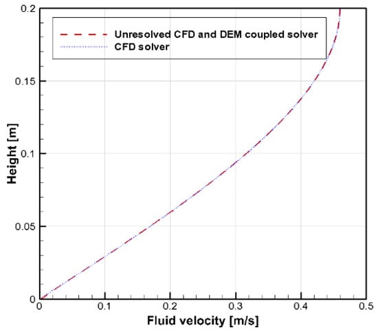
Figure 2.
Velocity profile by unresolved CFD and DEM solver, and CFD solver.
Table 2 shows the simulation parameters. A total number of 134,285 particles was used to form the seabed. The density of the particles was 2600 kg/m3. Young’s modulus and Poisson ratio of the particles were Pa and 0.45, respectively. The friction and rolling friction coefficients were 0.6 and 0.125, respectively. The time step for the CFD and DEM solvers were s and s, respectively. Every forty steps, both CFD and DEM results were coupled. The computational time for a single test took 10 days on a workstation equipped with Intel Xeon(R) Gold 6226R CPU 2.9 GHz processors.
Table 2.
Simulation parameters.
4. Numerical Model Parameters
4.1. Angle of Repose for Glass Beads
To verify the numerical methods, the angle of repose for glass beads was simulated. Figure 3 shows the geometrical specifications of the baseplate and hopper. The diameters of top and bottom of the hopper were 250 mm and 50 mm, respectively. The height of the hopper was 400 mm, and the diameter of the baseplate (Db) was 500 mm. The hopper moved slowly and vertically up from the initial position with a certain speed. The particles discharged from the hopper, accumulated on the baseplate, and gradually expanded to the edge [47].
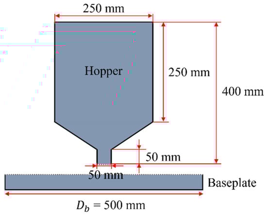
Figure 3.
Illustration of experimental set up for angle of repose [47].
The properties of the particles [47] are summarized in Table 3. The diameter (), density (), Poisson’s ratio (), and Young’s modulus () were 10 mm, 2500 , 0.24, and Pa, respectively. The total number of 13,000 particles were used. The measured sliding friction coefficient of the glass beads was 0.142, and the coefficient of rolling friction was assumed to be very small [47].
Table 3.
Simulation parameter for angle of repose.
Figure 4 shows the particle motions in the simulation of the angle of repose. The hopper filled with the particles elevated at 5 mm/s, and the gravity particles was discharged. The hopper was stopped at 110 mm height from the baseplate. The simulation was continued until the particles in the hopper were completely released and the pile was in a steady state. Then the number of particles of the stabilized pile () were obtained. The slope of the stabilized pile was not symmetrical because the released particles from the hopper were not symmetrical, causing the relative motion between the particles at the bottom of the pile and baseplate [48].
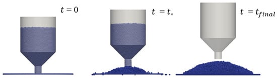
Figure 4.
Simulation of angle of repose for glass beads.
The angle of repose () could be calculated as:
where H indicates the height of the pile, and Db is the baseplate diameter. Table 4 lists the predicted angle of repose and number of the particles of the stabilized pile. The simulation result showed that the angle of repose and number of particles of the stabilized pile agreed well with the experimental data [47].
Table 4.
Angle of repose.
4.2. Angle of Repose for Sand Particles
In the experiment, non-spherical particles were used. While spherical particles were used in the present study. To simulate the behavior of non-spherical particles by the spherical particles, the coefficient of rolling friction should be adjusted. To decide the rolling friction coefficient () used in the scour simulation, a parametric study for the angle of repose for sand particles was carried out. The sand particle diameter was 1 mm. The density of the particles was 2600 kg/m3. Figure 5 shows the sand particle motions in the simulation of the angle of repose. The particles were discharged from the hopper [34]. Table 5 lists the rolling friction coefficients for a sliding friction coefficient. For the sliding friction coefficient, 0.6 was selected. This is because that sliding friction coefficients higher than 0.4 did not show a dominant effect on the angle of repose [48]. The angle of repose increased with increasing rolling friction coefficient. When the sliding friction coefficient was 0.6 and rolling friction coefficient was 0.125, the angle of repose () was 32.02°, which corresponded to the angle of repose of the sand [3,49]. From the simulation results, the sliding friction coefficient of 0.6 and rolling friction coefficient of 0.125 were selected.
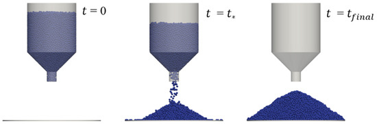
Figure 5.
Simulation of angle of repose for sandpile.
Table 5.
Angle of repose for various friction coefficients.
4.3. Incipient Motion of Sand Particles
The incipient motion of sand particles was simulated to validate interactions between the fluid flow and seabed particles. The computational domain for the unresolved CFD and DEM coupled solver is described in Figure 6. The sand particles with a diameter of 1 mm were randomly distributed and densely packed in the seabed region of 4 D length, 1 D width, and 0.25 D depth. The inlet boundary with 4 D height was specified with a uniform flow. The inlet velocity was raised up linearly to target velocity over first 1 s for a numerical stability. The results of the particle motion were presented, at the same time, after the first 1 s. All simulations for the incipient motion were carried out with the same seabed particle arrangement.
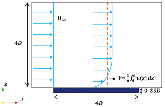
Figure 6.
Computational domain for incipient motion.
The incipient motion of the sand particles was determined using the criteria of Kramer [50]. Figure 7 shows the particle motion for various inlet velocities () in the region between x/D = 2.125 and 4. Figure 7a shows no particle motion at = 0.3 m/s. The motion of very few particles was initiated at isolated spots at = 0.4 m/s. At = 0.5 m/s, several particle motions occurred. The particle motions were increased with increasing inlet velocity, and the particles were moved in groups in the flow direction. According to Kramer [50], a level of weak movement was recommended as the incipient motion of the particles [51]. The weak movement represented the motion of small particles at isolated spots, which corresponded to the result in Figure 7b. In detail, the particle motion within the weak movement level is shown in Figure 8. As the inlet velocity () increased from 0.4 m/s to 0.52 m/s, and the number of moving single particles increased, forming groups with surrounding particles. When single particles sporadically formed groups, it could be considered a transition from the weak level to the medium level.
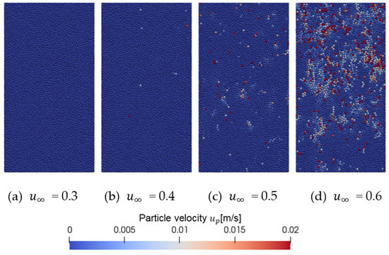
Figure 7.
Incipient motion of particles. The upper side and lower side indicate x/D = 2.125 and x/D = 4, respectively. (a) m/s; (b) m/s; (c) m/s; (d) m/s.
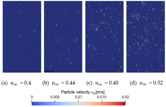
Figure 8.
Particle motion in weak level. The upper side and lower side indicate x/D = 2.125 and x/D = 4, respectively. (a) m/s; (b) m/s; (c) m/s; (d) m/s.
The Hjulstrom diagram [52] was employed to define the critical states of the particle motion, which could be used to distinguish between the transport, erosion, and deposition of sediments using the particle size and mean flow velocity. The inlet velocity () was not appropriate to characterize the flow situation for the sediment transport because the velocity profile changed over the length scale [53]. The mean flow velocity was defined as the depth-averaged velocity () at the central location in the x/D = 2.125. Here, is the top of the seabed surface. The mean flow velocity (V), which corresponded to the weak movement, ranged from = 0.4 m/s to 0.48 m/s and was calculated and indicated in the Hjulstrom diagram. Figure 9 shows the computed depth-averaged velocities with the particle diameter of 1 mm. The simulation results showed that it was predicted close to the critical velocity for the incipient motion of the particle.
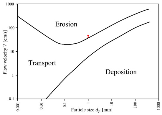
Figure 9.
Simulation results for = 1 mm in the ranged from = 0.4 to 0.48 m/s.
5. Results and Discussion
Simulations for scour around a subsea pipeline were carried out using the numerical methods used in the simulations of the angles of repose and incipient motion of the particles. A grid sensitivity study was performed using three different cases in Table 6. Here, 1, 2, and 3 represent coarse, medium, and fine grids, respectively. The total number of the grid was increased by 2 times. A representative grid size () was used [54]. The refinement factor for the representative grid size was . The particle size () was set consistently to 1 mm for the three cases. As the grid system was fined, the scour depth and drag force acting on the pipeline were converged. The drag coefficient showed the difference less than 5% [55]. The scour depth was converged in the case 2.
Table 6.
Grid sensitivity result.
The evolution of scour depth with time is shown in Figure 10. The depth of the scour hole () was normalized by the pipeline diameter (). The simulation results in the early stage of scour slightly underestimated the scour depth, in which the inlet velocity was gradually increased [38]. In other words, the onset of scour was postponed, due to a low velocity, which corresponded to about s. The scour depth increased sharply after the onset of scour, which corresponded to the tunnel erosion (about s). After the tunnel erosion, the scour depth increased at a relatively lower rate, which corresponded to the lee-wake erosion (about s). Additionally, the scour depth reached the equilibrium state. This trend was consistent with the experimental results [3]. In Yang et al.’ simulation [38], the scour depth predicted lower than the experimental data in the onset of scour and tunnel erosion. While the scour depth was in good agreement with the experimental data in the lee-wake erosion, the selection of the coefficient of rolling friction by the validation test in this study more accurately influenced the prediction in the onset of scour and tunnel erosion.
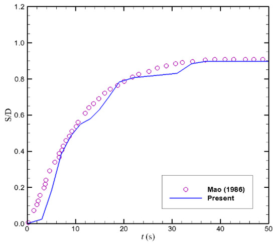
Figure 10.
Evolution of scour depth.
Figure 11 shows the evolution of a bed profile with time. The onset of scour was occurred at about s. The onset of scour was initiated by the seepage flow beneath the pipeline and pressure difference between the upstream and the downstream around the pipeline [7]. In the single-phase models, and some two-phase models, it was challenging to reproduce the onset of scour without a very small gap between the seabed bottom and the pipeline [13,19]. After the onset of scour, the tunnel erosion proceeded to < 0.3 (about s), due to an increase in fluid flow entering the opening beneath the pipeline. The eroded particles beneath the pipeline formed a sand dune about half the diameter of the pipeline downstream. During the scour process, a large amount of particle movement at the rear side of the pipeline occurred at the lee-wake erosion (about s). In addition, the scour hole was deepened and expanded downstream, while the sand dune moved farther and flattened in the direction of flow. These phenomena were consistent with the experimental observations [3,7].
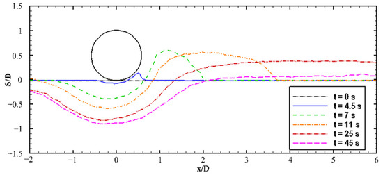
Figure 11.
Evolution of bed profile.
Figure 12, Figure 13, Figure 14, Figure 15 and Figure 16 show the results at the three stages of scour ( s). Figure 12 shows the contours of the fluid velocity normalized by the inlet velocity. In the onset of scour, the small velocity of the flow in the opening beneath the pipeline appeared. In the tunnel erosion, the small opening beneath the pipeline expanded into the tunnel, due to the increased flow. In the lee-wake erosion, the flow was affected by the seabed, and the deformed seabed region could be observed.
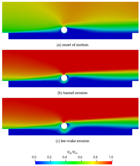
Figure 12.
Fluid velocity contours.

Figure 13.
Velocity of particles.
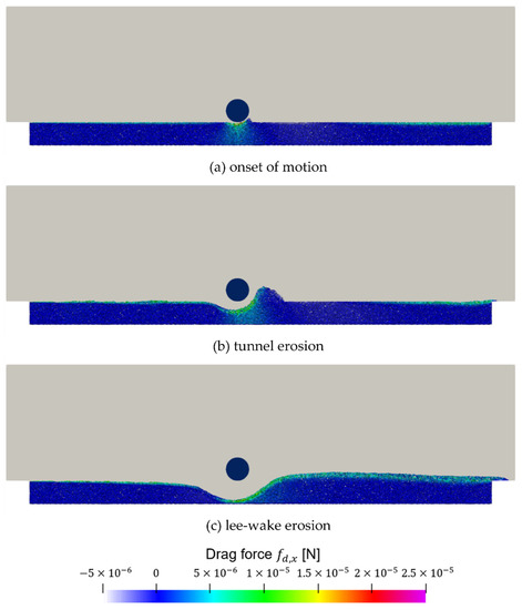
Figure 14.
The x-directional particle drag force ().
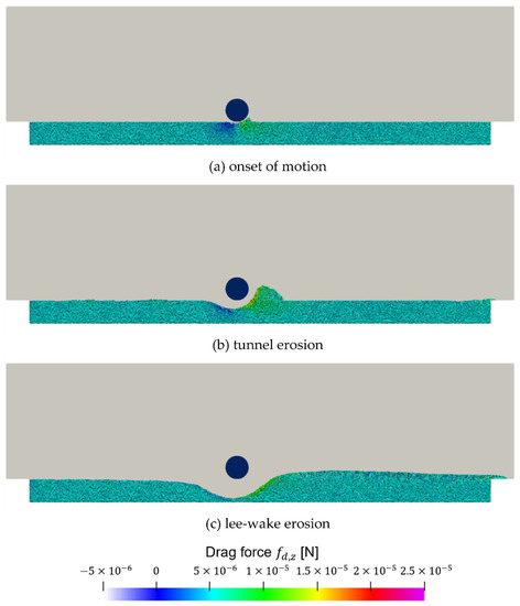
Figure 15.
z-directional particle drag force ().
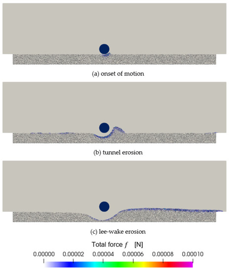
Figure 16.
Total force distribution ().
Figure 13 shows the velocity of the individual particles. The particles beneath the pipeline started to move at the onset of scour ( s). In the tunnel erosion ( s), the movement of the particles and number of moving particles around the pipeline were increased, indicating that the seabed under the pipeline was exposed to a strong erosion. In the lee-wake erosion ( s), the particles in the scour hole showed small movement, while the particles in the downstream of the scour hole moved in the flow direction.
The drag force is the dominant force in the fluid and particle interaction. Figure 14 shows the drag force acting on the individual particles in the flow direction. Until the tunnel erosion, the drag force increased mainly beneath the pipeline, causing the high scour depth rate. In the lee-wake erosion, the drag force applied to the seabed led to the expansion of the scour hole and the movement of many particles. The particle transport capacity in the scour process increased with the increase of the drag force. Figure 15 shows the drag force acting on individual particles in the vertical direction. The drag force acting in the vertical direction on the front and rear sides of the scour hole increased at the early stages and drove the motion of particles on the inclined bed inside the scour hole. From the results, the drag force acting on the particles played an important role in the transport of the sand particles.
Figure 16 shows the total force of the seabed particles. As the particles moved during the scour process, the interaction between the particles increased. In the region where the particle transport was most active, the interaction force between the particles was also the most intense. In Figure 13, Figure 14 and Figure 15, it was shown that the particle transport was most affected by drag force acting on the particles. However, it should be noted that the particle and particle interaction was also active in the rear side of the sand dune, where the drag force was not dominant. It concluded that the interaction between the particles should be considered in the development process of the scour hole and sand dune in the tunnel erosion. These results show why the CFD and DEM coupled model is more suitable than the single-phase model for scour simulation.
6. Conclusions
In this study, the simulations were carried out on scour around the seabed pipeline, in order to investigate the applicability of the CFD and DEM coupled solver [33]. The unsolved CFD and DEM coupled solver was used to track the particle motion caused by the fluid flow. For the verification of the numerical methods, the angles of repose were simulated and compared with the experimental data. The predicted angles of repose were in good agreement with the experimental data, and the rolling friction coefficient of the sand particles was decided for the scour simulation. The rolling friction coefficient should be used to compensate for non-spherical sand particles and determine the proper value for application to scour simulation. To validate the selected numerical model parameters, the incipient motion was simulated and discussed the critical state to validate the interaction between the fluid flow and seabed particles. The incipient motion of the sand particles was predicted close to the critical velocity in the Hjulstrom diagram.
The scour simulations around the subsea pipeline were carried out and compared with the experimental data [3]. From the grid dependency test, the CFD and DEM coupled solver could be applied without grid dependency constraints. The flow fields and interactions between the flow and particle were presented in the three scour stages. At the onset of the scour stage, the sand particles beneath the pipeline started to move, due to the seepage flow and pressure difference between the upstream and downstream around the pipeline. During the tunnel erosion stage, the sediment transport was significantly increased with the increasing drag force, indicating that the seabed beneath the pipeline was exposed to the strong erosion. The strong erosion by the tunnel flow also expanded the scour hole and formed the sand dune. It was confirmed that the interaction between the particles was most active beneath the pipeline and in the sand dune during the tunnel erosion stage. With entering the lee-wake erosion stage, the particle movement was very small in the scour hole but very active when moving downstream. The main particle motions around the pipeline were generated by the drag force, due to the high flow velocity and the interaction between the particles.
The present CFD and DEM coupled solver required a lot of computational time, but all of the above findings can be explained from the information of each individual particle without using empirical formulas or solving constitutive equations, including sand concentration. The CFD and DEM coupled model showed great potential to simulate particle and particle interactions, as well as the fluid and particle interactions in previous research and the current study.
Author Contributions
Conceptualization, S.S. and S.P.; methodology, S.S. and S.P.; validation S.S. and S.P.; simulation, S.S.; formal analysis, S.S.; writing—original draft preparation, S.S.; writing—review and editing, S.S. and S.P.; visualization, S.S.; supervision, S.P. All authors have read and agreed to the published version of the manuscript.
Funding
This research was supported by the National Research Foundation of Korea (NRF-2021R1I1A3044639).
Institutional Review Board Statement
Not applicable.
Informed Consent Statement
Not applicable.
Data Availability Statement
Not applicable.
Conflicts of Interest
The authors declare no conflict of interest.
References
- Whitehouse, R. Scour at Marine Structures: A Manual for Practical Applications; Thomas Telford: London, UK, 1998. [Google Scholar]
- Fredsøe, J. Pipeline–Seabed interaction. J. Waterw. Port Coast. Ocean Eng. 2016, 142, 1–20. [Google Scholar] [CrossRef] [Green Version]
- Mao, Y. The Interaction between a Pipeline and Erodible Bed; Technical University of Denmark: Kongens Lyngby, Denmark, 1986. [Google Scholar]
- Dargahi, B. The turbulent flow field around a circular cylinder. Exp. Fluids 1989, 8, 1–12. [Google Scholar] [CrossRef]
- Chiew, Y.M. Prediction of maximum scour depth at submarine pipelines. J. Hydraul. Eng. 1991, 117, 452–466. [Google Scholar] [CrossRef]
- Guan, D.; Hsieh, S.-C.; Chiew, Y.-M.; Low, Y.M.; Wei, M. Local scour and flow characteristics around pipeline subjected to vortex-induced vibrations. J. Hydraul. Eng. 2020, 146, 04019048. [Google Scholar] [CrossRef]
- Chiew, Y.M. Mechanics of local scour around submarine pipelines. J. Hydraul. Eng. 1990, 116, 515–529. [Google Scholar] [CrossRef]
- Sumer, B.M.; Fredsøe, J.; Christiansen, N. Scour around vertical pile in waves. J. Waterw. Port Coast. Ocean Eng. 1992, 118, 15–31. [Google Scholar] [CrossRef]
- Sumer, B.M.; Fredsøe, J. The Mechanics of Scour in the Marine Environment; World Scientific Publishing Company: Singapore, 2002. [Google Scholar]
- Trygsland, E. Numerical Study of Seabed Boundary Layer Flow around Monopile and Gravity-Based Wind Turbine Foundations. Master’s Thesis, Norwegian University of Science and Technology, Trondheim, Norway, 2015. [Google Scholar]
- Park, S.; Song, S.; Wang, H.; Joung, T.; Shin, Y. Parametric study on scouring around suction bucket foundation. J. Ocean Eng. Technol. 2017, 31, 281–287. [Google Scholar] [CrossRef] [Green Version]
- Roulund, A.; Sumer, B.M.; Fredsøe, J.; Michelsen, J. Numerical and experimental investigation of flow and scour around a circular pile. J. Fluid Mech. 2005, 534, 351. [Google Scholar] [CrossRef]
- Liang, D.; Cheng, L.; Li, F. Numerical modeling of flow and scour below a pipeline in currents: Part II. Scour simulation. Coast. Eng. 2005, 52, 43–62. [Google Scholar] [CrossRef]
- Liu, M.M.; Lu, L.; Teng, B.; Zhao, M.; Tang, G.Q. Numerical modeling of local scour and forces for submarine pipeline under surface waves. Coast. Eng. 2016, 116, 275–288. [Google Scholar] [CrossRef]
- Engelund, F.; Fredsøe, J. A sediment transport model for straight alluvial channels. Hydrol. Res. 1976, 7, 293–306. [Google Scholar] [CrossRef] [Green Version]
- Paola, C.; Voller, V.R. A generalized Exner equation for sediment mass balance. J. Geophys. Res. Earth Surf. 2005, 110, F04014. [Google Scholar] [CrossRef]
- Zhao, E.; Dong, Y.; Tang, Y.; Sun, J. Numerical investigation of hydrodynamic characteristics and local scour mechanism around submarine pipelines under joint effect of solitary waves and currents. Ocean Eng. 2021, 222, 108553. [Google Scholar] [CrossRef]
- Liang, D.; Huang, J.; Zhang, J.; Shi, S.; Zhu, N.; Chen, J. Three-Dimensional Simulations of Scour around Pipelines of Finite Lengths. J. Mar. Sci. Eng. 2022, 10, 106. [Google Scholar] [CrossRef]
- Yeganeh-Bakhtiary, A.; Kazeminezhad, M.H.; Etemad-Shahidi, A.; Baas, J.H.; Cheng, L. Euler–Euler two-phase flow simulation of tunnel erosion beneath marine pipelines. Appl. Ocean Res. 2011, 33, 137–146. [Google Scholar] [CrossRef]
- Fraga, V.S.; Yin, G.; Ong, M.C.; Myrhaug, D. CFD investigation on scour beneath different configurations of piggyback pipelines under steady current flow. Coast. Eng. 2022, 172, 104060. [Google Scholar] [CrossRef]
- Li, J.; Tao, J. CFD-DEM Two-Way Coupled Numerical Simulation of Bridge Local Scour Behavior under Clear-Water Conditions. Transp. Res. Rec. 2018, 2672, 107–117. [Google Scholar] [CrossRef]
- Zhu, H.P.; Yu, A.B. Steady-state granular flow in a three-dimensional cylindrical hopper with flat bottom: Microscopic analysis. J. Phys. D Appl. Phys. 2004, 37, 1497. [Google Scholar] [CrossRef]
- Kloss, C.; Goniva, C.; Hager, A.; Amberger, S.; Pirker, S. Models, algorithms and validation for opensource DEM and CFD–DEM. Prog. Comput. Fluid Dyn. 2012, 12, 140–152. [Google Scholar] [CrossRef]
- Hager, A.; Kloss, C.; Pirker, S.; Goniva, C. Parallel resolved open source CFD-DEM: Method, validation and application. J. Comput. Multiph. Flows 2014, 6, 13–27. [Google Scholar] [CrossRef] [Green Version]
- Uhlmann, M. An immersed boundary method with direct forcing for the simulation of particulate flows. J. Comput. Phys. 2005, 209, 448–476. [Google Scholar] [CrossRef] [Green Version]
- Tsuji, T.; Higashida, K.; Okuyama, Y.; Tanaka, T. Fictitious particle method: A numerical model for flows including dense solids with large size difference. AlChE J. 2014, 60, 1606–1620. [Google Scholar] [CrossRef]
- Askarishahi, M.; Salehi, M.S.; Radl, S. Voidage correction algorithm for unresolved Euler–Lagrange simulations. Comput. Part. Mech. 2018, 5, 607–625. [Google Scholar] [CrossRef] [Green Version]
- Peng, Z.; Doroodchi, E.; Luo, C.; Moghtaderi, B. Influence of void fraction calculation on fidelity of CFD-DEM simulation of gas-solid bubbling fluidized beds. AlChE J. 2014, 60, 2000–2018. [Google Scholar] [CrossRef]
- Zhu, H.P.; Yu, A.B. Averaging method of granular materials. Phys. Rev. E 2002, 66, 021302. [Google Scholar] [CrossRef]
- Wu, C.L.; Zhan, J.M.; Li, Y.S.; Lam, K.S.; Berrouk, A.S. Accurate void fraction calculation for three-dimensional discrete particle model on unstructured mesh. Chem. Eng. Sci. 2009, 64, 1260–1266. [Google Scholar] [CrossRef]
- Jing, L.; Kwok, C.Y.; Leung, Y.F.; Sobral, Y.D. Extended CFD–DEM for free-surface flow with multi-size granules. Int. J. Numer. Anal. Methods Geomech. 2016, 40, 62–79. [Google Scholar] [CrossRef]
- Wang, L.; Ouyang, J.; Jiang, C. Direct calculation of voidage in the fine-grid CFD–DEM simulation of fluidized beds with large particles. Particuology 2018, 40, 23–33. [Google Scholar] [CrossRef]
- Song, S.; Park, S. Unresolved CFD and DEM Coupled Solver for Particle-Laden Flow and Its Application to Single Particle Settlement. J. Mar. Sci. Eng. 2020, 8, 983. [Google Scholar] [CrossRef]
- Zhao, J.; Shan, T. Coupled CFD–DEM simulation of fluid–particle interaction in geomechanics. Powder Technol. 2013, 239, 248–258. [Google Scholar] [CrossRef]
- Schmeeckle, M.W. Numerical simulation of turbulence and sediment transport of medium sand. J. Geophys. Res. Earth Surf. 2014, 119, 1240–1262. [Google Scholar] [CrossRef]
- Sun, R.; Xiao, H. CFD–DEM simulations of current-induced dune formation and morphological evolution. Adv. Water Resour. 2016, 92, 228–239. [Google Scholar] [CrossRef] [Green Version]
- Zhang, Y.; Zhao, M.K.C.S.; Kwok, K.C.; Liu, M.M. Computational fluid dynamics–discrete element method analysis of the onset of scour around subsea pipelines. Appl. Math. Modell. 2015, 39, 7611–7619. [Google Scholar] [CrossRef]
- Yang, J.; Low, Y.M.; Lee, C.H.; Chiew, Y.M. Numerical simulation of scour around a submarine pipeline using computational fluid dynamics and discrete element method. Appl. Math. Model. 2018, 55, 400–416. [Google Scholar] [CrossRef]
- Hu, D.; Tang, W.; Sun, L.; Li, F.; Ji, X.; Duan, Z. Numerical simulation of local scour around two pipelines in tandem using CFD–DEM method. Appl. Ocean Res. 2019, 93, 101968. [Google Scholar] [CrossRef]
- Yazdanfar, Z.; Lester, D.; Robert, D.; Setunge, S. A novel CFD-DEM upscaling method for prediction of scour under live-bed conditions. Ocean Eng. 2021, 220, 108442. [Google Scholar] [CrossRef]
- Cundall, P.A.; Strack, O.D. A discrete numerical model for granular assemblies. Geotechnique 1979, 29, 47–65. [Google Scholar] [CrossRef]
- Zhou, Y.C.; Wright, B.D.; Yang, R.Y.; Xu, B.H.; Yu, A.B. Rolling friction in the dynamic simulation of sandpile formation. Phys. A 1999, 269, 536–553. [Google Scholar] [CrossRef]
- Roessler, T.; Katterfeld, A. Scaling of the angle of repose test and its influence on the calibration of DEM parameters using upscaled particles. Powder Technol. 2018, 330, 58–66. [Google Scholar] [CrossRef]
- Ai, J.; Chen, J.F.; Rotter, J.M.; Ooi, J.Y. Assessment of rolling resistance models in discrete element simulations. Powder Technol. 2011, 206, 269–282. [Google Scholar] [CrossRef]
- Sweby, P.K. High Resolution Schemes Using Flux Limiters for Hyperbolic Conservation Laws. SIAM J. Numer. Anal. 1984, 21, 995–1011. [Google Scholar] [CrossRef]
- Lee, C.H.; Low, Y.M.; Chiew, Y.M. Multi-dimensional rheology-based two-phase model for sediment transport and applications to sheet flow and pipeline scour. Phys. Fluids 2016, 28, 053305. [Google Scholar] [CrossRef]
- Chen, H.; Liu, Y.L.; Zhao, X.Q.; Xiao, Y.G.; Liu, Y. Numerical investigation on angle of repose and force network from granular pile in variable gravitational environments. Powder Technol. 2015, 283, 607–617. [Google Scholar] [CrossRef]
- Nakashima, H.; Shioji, Y.; Kobayashi, T.; Aoki, S.; Shimizu, H.; Miyasaka, J.; Ohdoi, K. Determining the angle of repose of sand under low-gravity conditions using discrete element method. J. Terramech. 2011, 48, 17–26. [Google Scholar] [CrossRef]
- Li, F.; Cheng, L. Numerical model for local scour under offshore pipelines. J. Hydraul. Eng. 1999, 125, 400–406. [Google Scholar] [CrossRef]
- Kramer, H. Sand mixtures and sand movement in fluvial model. Trans. Am. Soc. Civ. Eng. 1935, 100, 798–838. [Google Scholar] [CrossRef]
- Buffington, J.M. The legend of AF Shields. J. Hydraul. Eng. 1999, 125, 376–387. [Google Scholar] [CrossRef]
- Hjulstrom, F. Studies of the Morphological Activity of Rivers as Illustrated by the River Fyris; Bulletin of the Geological Institution of the University of Upsala: Upsala, Sweden, 1935; pp. 221–527. [Google Scholar]
- Plenker, D.; Grabe, J. Simulation of sand particle transport by coupled CFD-DEM: First investigations. In Proceedings of the 8 International Conference on Scour and Erosion, Oxford, UK, 12–15 September 2016; Harris, J., Whitehouse, R., Moxon, S., Eds.; pp. 109–118. [Google Scholar]
- Celik, I.B.; Ghia, U.; Roache, P.J.; Freitas, C.J. Procedure for estimation and reporting of uncertainty due to discretization in CFD applications. J. Fluids Eng. 2008, 130, 078001. [Google Scholar]
- Pang, A.L.J.; Skote, M.; Lim, S.Y.; Gullman-Strand, J.; Morgan, N. A numerical approach for determining equilibrium scour depth around a mono-pile due to steady currents. Appl. Ocean Res. 2016, 57, 114–124. [Google Scholar] [CrossRef]
Publisher’s Note: MDPI stays neutral with regard to jurisdictional claims in published maps and institutional affiliations. |
© 2022 by the authors. Licensee MDPI, Basel, Switzerland. This article is an open access article distributed under the terms and conditions of the Creative Commons Attribution (CC BY) license (https://creativecommons.org/licenses/by/4.0/).