Multi-Scale Influence of Flexible Submerged Aquatic Vegetation (SAV) on Estuarine Hydrodynamics

Abstract

Bottom friction is an important process in coastal and estuarine environments because it can reduce wave heights and moderate tidal currents. When modeling large systems with spatially varying hydraulic properties, bottom friction values are commonly derived from land use classification products. However, estimation of bottom friction for vegetated areas can be more challenging due to the complicated and time-varying geometry of the roughness elements. This is particularly true of flexible, buoyant submerged aquatic vegetation (SAV) species, such as seagrasses and kelps, that deform under waves and currents. In this study we incorporate a dynamic friction model that includes the temporal variation in SAV drag forces into a depth-integrated coupled circulation-wave model. In vegetated areas, the bottom friction is continuously updated based on plant geometry, water depth, and combined wave-current velocities. Taking a multi-scale approach, we use the model to investigate the impact of SAV dynamics on both the localized and the integrated bay-wide hydrodynamics of a riverine and tidally influenced estuary. First, we investigate SAV modification of velocity fields and its implications for sediment transport and circulation pathways. Then, we show how SAV can modify tidal behavior throughout the estuary.

1. Introduction

The confluence of tides, wind, waves, and streamflow make estuaries one of the most hydrodynamically unique ecosystems [1]. The combination of terrestrial and oceanic forcings produces a wide array of commercially valuable services, including navigation, sustenance, and recreation [2,3]. Nearly all of these services depend on the balance between oceanic and terrestrial hydrodynamics, which dictates fluid and sediment fluxes. The ecological landscape of an estuary has also been shown to influence estuarine dynamics, such as reduction in tidal currents [4,5,6], tidal prism modification [7], as well as increased sediment retention [8]. Thus, quantifying changes to estuarine services under current and future climatologies requires accurate prediction of flow modification by vegetation canopies.

Restoration of natural and nature-based features (NNBFs) for ecological benefits and/or engineering services further necessitates understanding of the broader influence of vegetation on estuarine-scale hydro- and sediment dynamics. Due to the spatial scale variation between the study environment (O ∼ km) and the variability in vegetation features of interest (O ∼ cm-m), quantifying the sensitivity of estuarine hydrodynamics to vegetation conditions remains a challenge, especially for the case of buoyant, flexible submerged aquatic vegetation (SAV) species. We seek to fill a methodological gap to efficiently and accurately quantify drag forces from flexible SAV in the flow field for regional hydrodynamic computational models.

1.1. Estuarine Hydrodynamics

At the oceanic boundary, astronomical tides play a leading order role in controlling estuarine processes. As they propagate inland, the tides interact with increasingly shallower bathymetry, resulting in a combination of amplification (shoaling), reflection off the side walls, and dissipation (amplitude decay) by bottom friction and turbulent mixing [9,10,11]. Bottom friction and nonlinear interactions also produce higher-order harmonic overtides that result in time-averaged tidal asymmetry [12,13]. In shallow and/or long estuaries dominated by bottom friction, flood tide energy dissipates with distance into the estuary and reduces the intensity of the ebbing tide [10,14,15]. Such systems are referred to as flood-dominant and result in landward mean sediment transport [15,16]. In contrast, deeper channels (via reduced drag) and shorter channels (via resonance) tend to be ebb-dominant and lead to mean sediment export as tidal energy is amplified [14,15,17]. Flood and ebb dominance can vary throughout a tidal basin depending on local bathymetry and proximity to river discharge [15,18]. Strong riverine discharge at the landward boundary can also de-correlate tide duration asymmetry and peak current asymmetry because riverine discharge opposes flood tide propagation while simultaneously enhancing ebb tide current velocities [16,18,19].

Enhanced bottom friction due to vegetation has been shown to shift tidal asymmetry [20,21,22]. Although increased bottom friction can lead to decreased tidal amplification, there is some dependence on estuarine shape that determines whether a system with enhanced friction remains hypersynchronous (tidal amplification with up-channel propagation) or becomes hyposynchronous (tidal dampening with up-channel propagation) [19]. Reduced tidal current velocities due to bottom roughness may also shift flow pathways and estuarine circulation. Additionally, reduction in tidal and wave-driven velocities by SAV habitats can have impacts at the local scale as well, including a decreased tendency for sediment transport (e.g., reduction in shoreline erosion) and increased shelter for fishery juveniles [23,24].

1.2. Vegetation-Induced Bottom Friction

The presence of vegetation in coastal environments reduces the momentum of the ambient flow, predominantly by overcoming a drag force acting on the plant’s stems and leaves [25]. Approximating a single plant as a rigid cylinder, the drag across the plant can be formulated using a quadratic drag law $\frac{1}{2}{C}_d\rho b{l}_v{U}^2$, where $C_d$ is the drag coefficient, $\rho$ is the fluid density, U is the flow velocity, and b and $l_v$ are the plant’s width (or diameter, depending on plant morphology) and height, respectively [26]. Analytical solutions of vegetation-induced drag have been incorporated into coastal circulation models [6,27] and spectral wave models [28,29,30], which has enabled the study of their control on hydrodynamics across regional scales. Formulations of vegetation drag that are a function of plant geometry minimize the need to empirically parameterize drag forces. However, variation in natural plant geometry from the rigid cylinder approximation complicates the determination of $C_d$ [26]. Various studies have shown that $C_d$ values for vegetation can be predicted from the flow Reynolds number ($Re$) [31,32,33], the Keulegan–Carpenter number ($KC$) [34,35], and vegetation canopy geometry [34,36], but multi-factor models of $C_d$ for vegetation in combined wave-current flows have not yet converged to a singular approach [37,38]. Even more so than the drag coefficient, accurate calculation of drag forces has been shown to depend strongly on the height and vertical distribution of the vegetation of interest [4,39,40].

In contrast to calculating the vegetation ‘sink’ term by explicitly modeling drag over individual stems, an alternative approach can be derived using hydraulics, whereby vegetation is interpreted as a form of surface roughness in aggregate. Using this more implicit form of bottom friction to estimate vegetation-induced drag forces is particularly advantageous for depth-averaged circulation models because it can be adapted to all land cover types and it enables large scale parameterization efficiently [8,41,42,43,44,45]. Mapping of Manning’s n bottom roughness coefficients from land use and land cover (LULC) datasets has become a common methodology for determining Manning’s n across a regional study environment [46,47,48]. However, the flexibility afforded by landscape-to-roughness mapping comes at a cost of precision and accuracy as bottom roughness can vary considerably at scales smaller than available LULC geospatial products, which also generally do not capture subaquatic features.

While there are significant advantages and disadvantages to both the explicit and implicit methods of modeling momentum loss due to flow-vegetation interactions, neither approach accounts for the variability of flow resistance by SAV due to its flexibility and deflection under waves and currents [49,50,51]. In order to fully capture the dynamic feedback between fluid drag forces and vegetation motion, three-dimensional (3D) or quasi-3D modeling techniques are required. To date, only a handful of community coastal models are available to study 3D vegetation-induced drag, turbulence, and wave streaming effects for deformable explicit vegetation stems [27,52], but they are substantially more computationally intensive than 2D depth-averaged (2DH) models. Furthermore, it is critical for more open-source models to rely on physics-based parameterizations to improve estimation of ecosystem services for large regions and to improve inter-model comparisons [53].

We explore the importance of sub-grid vegetation hydrodynamics to estuarine- and regional-scale circulation modeling. We modify commonly used, open-source circulation and wave models to allow flexible SAV to be parameterized as time-varying bottom friction. We then apply the model to an estuary with large SAV-inhabited tidal flats to assess how sensitive hydrodynamic quantities are to vegetation parameterization schemes. Rather than relying on empirical tuning, our dynamic parameterization scheme pulls directly from leading developments in the field of SAV behavior under waves and currents. We then apply the new method to our study site in Coos Bay, Oregon to demonstrate canopy-scale control on velocity fields, circulation patterns, and tidal characteristics.

2. Methods

First, we present our estuary of study. Then, we describe in detail the numerical modeling methods and forcing conditions used, paying greatest attention to the novel dynamic friction routine we developed. Finally, we briefly describe the numerous analytical methods used to quantify hydrodynamic statistics of interest from modeled output, as they are well documented in the literature elsewhere. We calculate both local and integrated quantities to illustrate the breadth of influence of the newly developed dynamic friction routine.

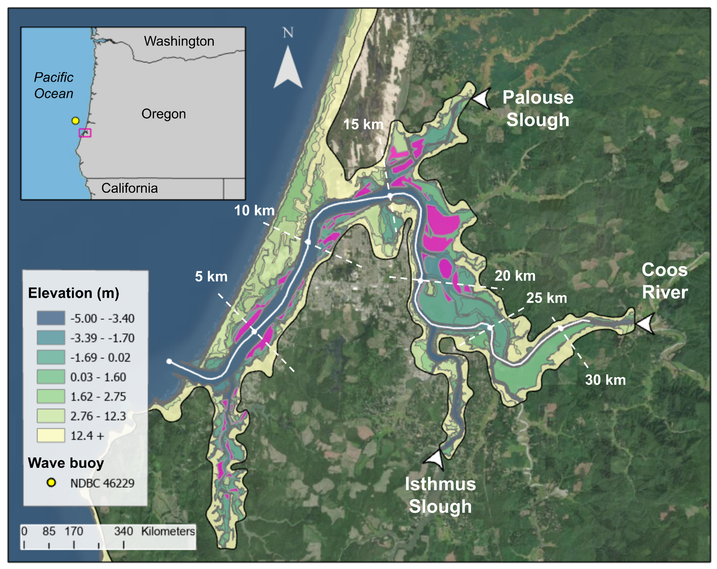
2.1. Study Site—Coos Bay Estuary

We center our numerical sensitivity study on the Coos Bay Estuary (CBE), located on the Oregon (USA) coast (Figure 1). The CBE is one of the largest estuaries on the US Pacific coast [54,55]. The bathymetry of the estuary has evolved considerably since the Euro-American displacement of native tribes for the extraction of local resources [56]; work by Eidam et al. [55] and Eidam et al. [57] illustrates how anthropogenic modifications to the CBE’s bathymetry have changed tidal and sediment dynamics over time. Presently, the estuary is 44 km${}^2$ in size, approximately half of which is intertidal [54,58,59,60]. Wide tidal flats support approximately 6.9 km${}^2$ of SAV habitat [24,61], making the CBE one of the most SAV-rich Oregon estuaries and an ideal site for our numerical experiment. Selection of the CBE is also particularly apt due to the fact that it has been the focus of several recent studies [55,57,60,62].

In the CBE, both terrestrial- and oceanic-derived forcings exhibit a strong seasonal signal. The bay is fed by several freshwater sources with seasonally varying flowrates, peaking in winter months and lowest in summer. The predominant source of freshwater is the Coos River with an average winter (December, January, February; DJF) flowrate of 86.6 m${}^3$/s and average summer (June, July, August; JJA) flowrate of 9.87 m${}^3$/s. Additional flows from Palouse Slough to the north and Isthmus Slough to the southwest of the Coos River supply between 1.64 m${}^3$/s and 0.11 m${}^3$/s (DJF and JJA seasonal averages) and between 3.44 m${}^3$/s and 0.10 m${}^3$/s, respectively [63,64]. Winter peaks in streamflow also coincide with stronger offshore wave intensities, with significant wave heights $H_s$ of 3.01 m and peak wave periods $T_p$ of 12.6 s oriented nearly shore-normal; in the summer, waves arrive northwesterly (NW) with $H_s$ of 1.55 m and $T_p$ of 9.39 s (NDBC Station 46229).

Figure 1. Site map of the CBE [65]. SAV habitats used to parameterize the ADCIRC+SWAN model shown in magenta. Riverine flow points shown with white arrows. White dashed lines correspond to along-channel distance landward of the CBE inlet ($dx$).

Figure 1. Site map of the CBE [65]. SAV habitats used to parameterize the ADCIRC+SWAN model shown in magenta. Riverine flow points shown with white arrows. White dashed lines correspond to along-channel distance landward of the CBE inlet ($dx$).

2.2. Numerical Model

In this study, we embed a dynamic bottom friction routine into the open-source finite element coastal circulation model ADCIRC coupled with the spectral wave model SWAN [30,66,67]. The depth-averaged mode of ADCIRC has been used for numerous regional studies of estuarine hydrodynamics as well as for modeling impacts of compound storm events [60,68]. When coupled with SWAN, ADCIRC is highly computationally efficient and parallelizable, making ADCIRC+SWAN an excellent model choice for compound-forced estuary modeling [60,67]. Our study on the sensitivity of modeled velocities and tidal constituents to dynamic bottom friction builds on existing literature on the bottom friction sensitivity of the ADCIRC and coupled ADCIRC+SWAN models [47,48,69,70,71].

For our numerical sensitivity experiment, we rely on a previous calibration of the computational mesh performed by Parker et al. [60] because it was found to be a faithful representation of the dominant physical drivers of hydrodynamics within the CBE, including the compound interaction of tides, waves, wind, and streamflow ($R^2>0.97$ for a month-long validation period). Topo-bathymetric elevations are sourced from a blend of DEMs from National Oceanic and Atmospheric Administration and LiDAR surveys taken by the Oregon Department of Geology and Mineral Industries. The mesh is made up of about 30,000 computational nodes, and triangular grid cell sizes range from 10 m (small channels) to 150 m throughout the bay itself. Outside of the bay, computational cell size increases to over 3 km at the tidal forcing boundary (located 133 km offshore).

2.3. Boundary Conditions

Water surface elevations at the offshore boundary are prescribed by the eight dominant tidal harmonics for the region; harmonic amplitudes, frequencies, and equilibrium arguments are extracted from the TPXO tidal database [72] using the OceanMesh2D MATLAB toolkit [73]. Offshore wave, wind, and streamflow conditions are modeled on seasonally averaged winter (DJF) conditions (

Table 1. Hydrodynamic forcing conditions for Coos Bay Estuary model.

	Value	Data Sources	Record Length
Waves	JONSWAP	NOAA NDBC	2005–2013
$H_s$ (m)	3.01
$T_p$ (s)	12.6
${\varphi }_w$ (deg)	275
Wind
Daily $W_{max}$ (m/s)	4.10	NOAA NWS WRCC	1996–2006
Daily $W_{min}$ (m/s)	3.86	ISU IEM	1949–Present
Mean ${\varphi }_W$ (${}^{\circ }$)	166	NCEP NCARR	1981–2010
Streamflow (m${}^{\mathbf{3}}$/s)		USGS Streamstats	1906–2005
Coos River	86.6
Isthmus Slough	3.44
Palouse Slough	1.64

). In addition to tides, the open ocean boundary nodes are forced with a temporally and spatially uniform JONSWAP spectrum parameterized by historical wave observations collected at NDBC Station 46229. Spatially uniform wind fields are applied over the domain to maintain wave heights as they propagate from the open boundary towards the bay.

Wind magnitudes and directions were determined from multiple data sources, including observations at the North Bend Airport [74,75] and long-term averaged wind reanalysis products by NCEP NCAR [76]. Wind velocities are assumed to be spatially uniform over the domain but do oscillate diurnally due to their dependence on the solar heat flux. Finally, constant streamflow rates are defined as the DJF average of the median monthly flow rates at each of the riverine boundaries; flow-duration statistics are derived from linear multiple regression analysis of streamflow records between 1906 and 2005 developed by USGS StreamStats [63,64].

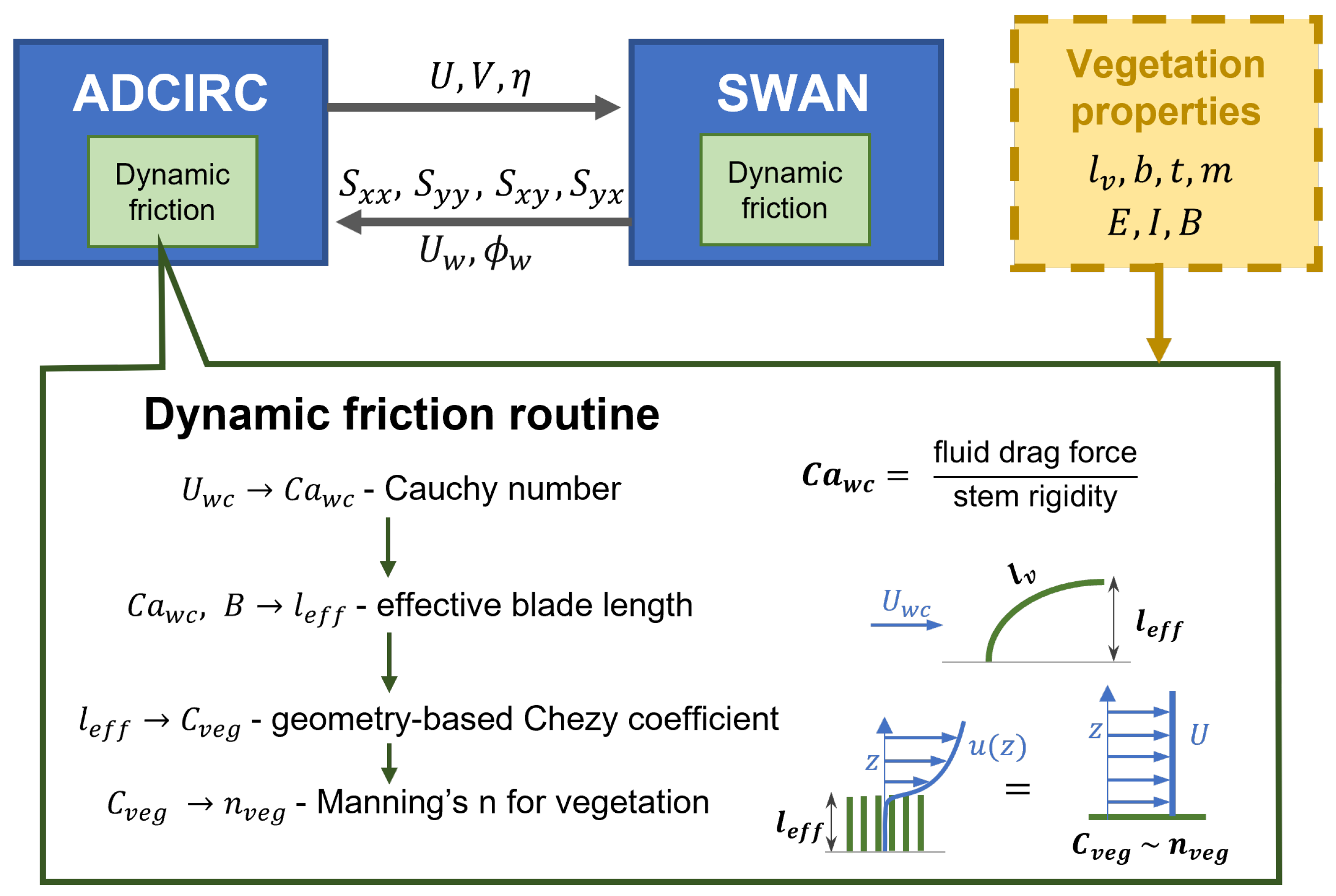
2.4. Dynamic Bottom Friction

Using time-varying computed current velocities, wave statistics, and model SAV properties, we compute a dynamically varying Manning’s n value in SAV habitats, or $n_{SAV}$, at each time step for every node classified as SAV. A schematic of the ADCIRC+SWAN information exchange and the dynamic friction routine is shown in Figure 2. The arrows between the solid blue boxes in Figure 2 represent the tight coupling between ADCIRC, which calculates depth averaged velocities ($U,V$) and water surface elevation ($\eta$), and SWAN, which passes to ADCIRC wave radiation stresses ($S_{xx},S_{xy},S_{yx},S_{yy}$). To calculate the combined wave-current drag on our computational SAV, the time-varying root mean square ($rms$) wave velocity $U_w$ and mean direction ${\varphi }_w$ are also passed from SWAN to ADCIRC.

The dynamic friction routine inserted in both ADCIRC and SWAN (Figure 2) uses a physically representative vegetation-induced bottom roughness formulation proposed and validated by Baptist et al. [77]. Developed using data-driven genetic programming, the roughness formulation is trained on results of a $k-\epsilon$ turbulence model of submerged canopy flow [78]. Assuming the bottom roughness of the bare bed is negligible relative to the roughness caused by the vegetation, the Chezy coefficient C is defined as

$$C=\sqrt{\frac{2g}{C_{d}mb{l}_v}}+\frac{\sqrt{g}}{\kappa }ln\left(\frac{h}{l_v}\right)$$

(1)

where m is the density of vegetation within the canopy (blades/m${}^2$), h is the water depth, g is the acceleration due to gravity, and $\kappa$ is the von Karman coefficient.

Because the formulation for C by Baptist et al. [77] depends on SAV height, we account for nonstationary plant posture by calculating the effective height $l_e$ of the deflected plant, which can be predicted from two dimensionless parameters, the Cauchy number ($Ca$) and the buoyancy parameter (B) [79]. $Ca$ is used to quantify the posture-dependent ratio of drag forces to plant stiffness. The relationship between the effective height and $Ca$ is modulated by B. In summary, these two dimensionless numbers quantify the response of a plant stem or blade to the flow as a function of its total resistance to motion (buoyancy and stiffness). The expression for $l_e$ developed and validated by Luhar and Nepf [79] is

$$\frac{l_e}{l_v}=1-\frac{1-0.9C{a}^{-1/3}}{1+C{a}^{-3/2}(8+B^{3/2})}$$

(2)

and the dimensionless parameters $Ca$ and B are defined as

$$Ca=\frac{C_d\rho b{U}^2{l}_v^3}{2EI}$$

(3)

$$B=\frac{({\rho }_v-\rho )gbt{l}_v^3}{EI}$$

(4)

where E is the modulus of elasticity, I is the moment of inertia about the rotational axis (equal to $b{t}^3/12$), ${\rho }_v$ is the density of plant material, and t is the stem or blade thickness.

For our study, the numerical dynamic vegetation is modeled after the SAV species Zostera marina (Z. marina). Because previous field surveys of Z. marina in the CBE have been limited [24], we defined the geometric and mechanical properties of our SAV mimic using the mean values of properties published in surveys of Z. marina in PNW estuaries [59,80,81,82,83,84,85,86]. Values of the necessary Z. marina parameters are an additional input to the dynamic friction routine (dashed yellow box in Figure 2); the specific values used for our numerical experiment are shown in Nomenclature.

Although ADCIRC allows the bottom boundary to be parameterized with C, we use the Manning’s n formulation, which can be found from the Chezy coefficient via $n=h^{1/6}/C$. By substituting the equation of effective height $l_e$ (Equation (2)) for $l_v$ in Equation (1), we can translate sub-grid flow-vegetation interactions into a framework easily interpreted by friction-based numerical models. We will rely on the Luhar and Nepf [79] model of plant deflection that is a function of $Ca$ for the combined wave-current flow magnitude, $U_{wc}$,

$$U_{wc}=\sqrt{U_0^2+U^2+2U_0\left|U\right|cos\left(|{\varphi }_c-{\varphi }_w\right|)}$$

(5)

where $U_0$ is the near-bed wave orbital velocity equal to $\sqrt{2}{U}_w$ and ${\varphi }_c$ and ${\varphi }_w$ represent the approach angle of the current and wave velocities, respectively (${\varphi }_c=\mathrm{atan}2(V,U)$) [87]. Thus, our approach retains dependence on plant buoyancy as well as the wave environment in the event that $U_w>>U$. Based on Luhar and Nepf [79], we assume that $C_d$ for a deflected plant stem is adequately described by the drag over a rigid cylinder with equivalent height of the deflected stem; essentially, once the effective plant height is known, calculations of drag based on a rigid cylinder assumption are valid. In this work, we assume a constant $C_d$ of 1.0 [88]. Finally, we impose a maximum $n_{SAV}$ value of 0.10, which prevents $n_{SAV}$ from becoming unrealistically high [89].

Because bottom friction in SWAN is parameterized with the wave bottom friction factor, $f_w$, ADCIRC first converts Manning’s n values to an equivalent roughness height, $z_0$ [67,90]. SWAN converts $z_0$ to $f_w$ and then an equivalent friction coefficient, $C_b$, which modulates the bottom friction dissipation term in the wave action balance [91]. Although SWAN also has an explicit vegetation module that adds an additional sink term based on formulations of drag over rigid cylinders [28,29,30], we are restricting the current work to not include additional vegetation modules at this time to maintain consistency across ADCIRC and SWAN, though its inclusion could be an important element of future research [92].

Our approach differs from other recent advances in vegetation drag for large-scale hydrodynamic modules because we account for both vegetation blade mechanics and deflection under waves and currents. For example, Moki et al. [93] calculate a spatially varying Manning’s n that is only dependent on SAV leaf morphology but does not account for plant deflection because their focus is on spatial variability of bottom roughness rather than temporal variability. Zhao and Chen [94] do incorporate a dynamic Manning’s n into a wave model, but their formulation is based on an iterative solution for n and the deflected vegetation height $l_e$ [95].

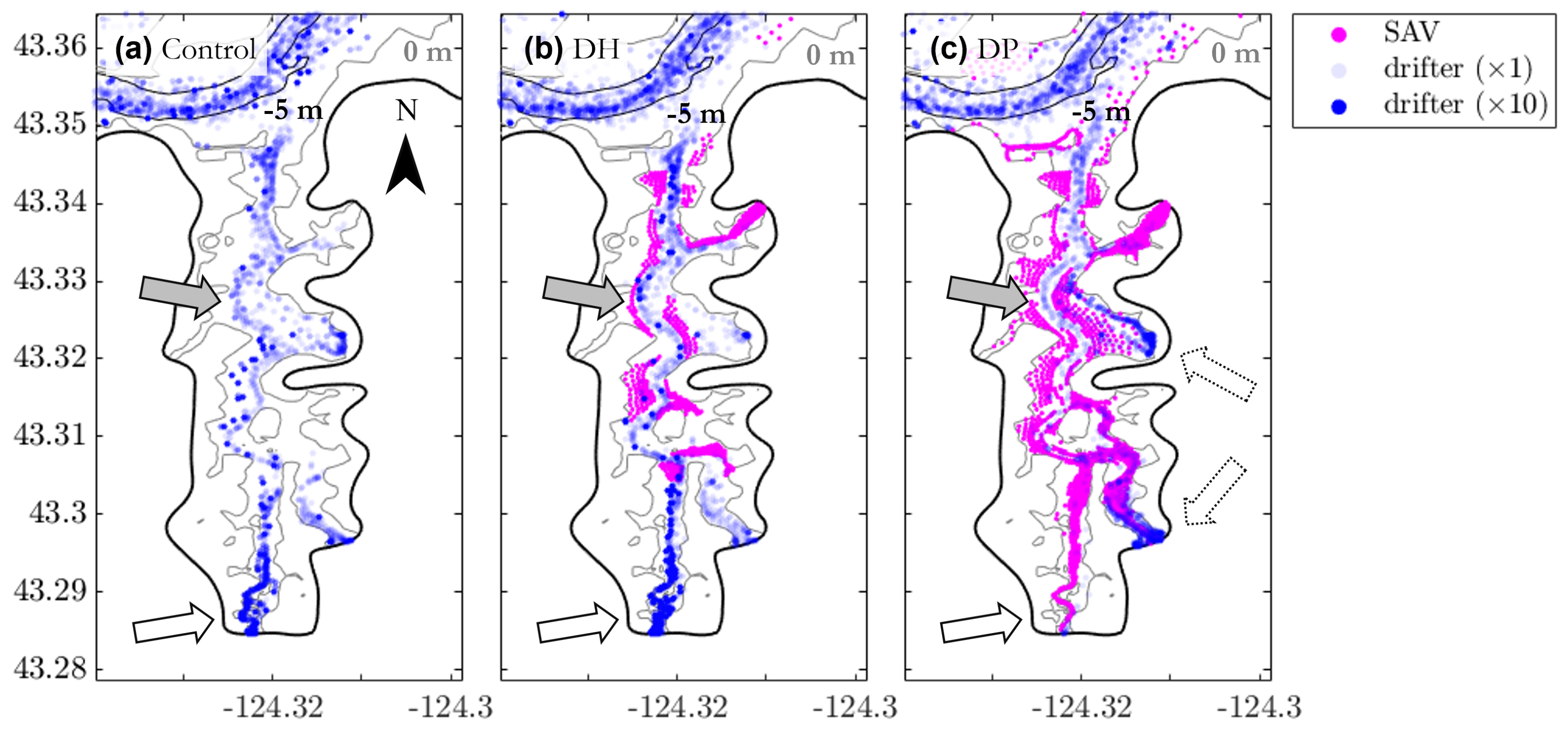
2.5. Experimental Design

We examine the effect of a dynamic $n_{SAV}$ on the hydrodynamics of the CBE by performing the same 40-day simulation with a number of bottom friction treatments in SAV habitats (

Table 2. SAV parameterization schemes implemented in ADCIRC+SWAN.

Treatment	ID	Coverage Extent	Spatially Varying?	Time Varying?	Description
Control	−	none	N	N	Friction values derived from LULC classification [60,96]
Status Quo	SQ	historic [24]	N	N	$n_{SAV}$ given empirically derived value (0.035) from published LULC-to-Manning’s n conversion tables
Dynamic Historic	DH	historic	Y	Y	$n_{SAV}$ calculated from dynamic friction routine (Figure 2)
Dynamic Potential	DP	potential [55]	Y	Y	$n_{SAV}$ calculated from dynamic friction routine (Figure 2)
Static Varying	SV	historic	Y	N	$n_{SAV}$ at each SAV node equal to time-averaged value from DH simulation
Static Uniform	SU	historic	N	N	$n_{SAV}$ at each SAV node equal to time- and space-averaged value from DH simulation

), each of which is compared with a control simulation where no SAV is included. In the control, SAV habitats are assigned a Manning’s n equivalent to that of a bare sediment bed (0.02); outside of SAV habitats for the control and all other simulations, n is assigned based on LULC classification [60,96]. The first SAV parameterization scheme used, referred to as the status quo treatment (SQ), represents the common approach of assigning a single, empirically derived value of $n_{SAV}$ based on LULC classification (equal to 0.035 for vegetated intertidal flats) [41,70,97,98]. The simplicity of the SQ treatment contrasts in complexity with the dynamic parameterization scheme, which applies the dynamic friction routine (Figure 2) to all nodes within the SAV habitats. This dynamic treatment is used for two different coverages of SAV, one with historical coverage [24] and one with potential coverage [55]. The former is referred to as the dynamic historic (DH) treatment, and the latter, the dynamic potential (DP) treatment, represents dynamic motion of SAV, should SAV be present in all locations designated as potential habitat based on light penetration thresholds ($z_{SAV}$ = −1 m < MLLW < 0.5 m [55]), which nearly doubles modeled SAV habitats from the historical extents.

Finally, to isolate the effect of temporal and spatial variability in $n_{SAV}$ on hydrodynamic observations, we re-perform the simulation with time- and space-averaged values of $n_{SAV}$ calculated during the DH simulation. For the static varying (SV) parameterization scheme, the value of $n_{SAV}$ at any given SAV node is equivalent to the time-averaged value of $n_{SAV}$ at the same node during the DH simulation. While the SV treatment of $n_{SAV}$ is spatially varying and temporally static, the static uniform (SU) parameterization is both temporally static and spatially uniform. All SAV nodes are given the identical value of $n_{SAV}$ for the SU treatment, equal to the time- and space-averaged value of $n_{SAV}$ across all SAV nodes in the DH simulation.

2.6. Analysis

2.6.1. Depth-Averaged Hydrodynamics

Depth-averaged horizontal current velocities $U,V$ are reported by ADCIRC at 15-min sampling intervals. Spectral wave statistics calculated by SWAN are also reported at 15-min intervals, including $H_s$, $U_w$, $T_p$, and ${\varphi }_w$. Using the simulated wave and current velocity fields, we first calculate the effect of SAV flow attenuation on the likelihood of localized sediment transport. Then, we use the simulated results to calculate the effect of SAV coverage on large-scale estuarine hydrodynamics, specifically tidal distortion and spatial patterns of flow circulation.

2.6.2. Sediment Fluxes

Non-cohesive sediments are predicted to be mobilized when the dimensionless transport number (Shields number, $\theta$) exceeds the critical Shields number ${\theta }_c$, defined as

$${\theta }_c=\frac{0.3}{1+1.2D_{*}}+0.055(1-e^{-0.02D_{*}}),\mathrm{and}$$

(6)

$$D_{*}=d_{50}{\frac{g(s-1)}{{\nu }^2}}^{1/3},$$

(7)

where $D_{*}$ is the dimensionless grain size, $d_{50}$ is the median grain size, s is the specific gravity of the material (equal to the ratio of the sediment to fluid density), and $\nu$ is the kinematic viscosity of water [99,100]. Spatially varying values of $d_{50}$ are interpolated to computational element centroids within the bay using samples collected by Eidam et al. [55]. Areas within the CBE made up of fine bed material ($d_{50}$ < 0.06 mm) are excluded from the analysis [99]. The tendency for transport was calculated for all sandy areas of the bay from the simulated current and wave velocities following [99,100],

$$\theta =\frac{C_b{U}_{wc}^2}{g(s-1)d_{50}}.$$

(8)

In Equation (8), $C_b$ represents the bed friction drag coefficient that varies with bed material type and relative depth [99].

2.6.3. Circulation

Passive tracer methods are commonly used to quantify an estuary’s residence time, also known as its turn-over time or flushing time [101,102]. Numerical implementations of particle tracking have also been used to investigate circulation and dispersal as an alternative to in situ drifter deployments, particularly for large estuaries with complex geometries. Advected pathways (latitude, longitude) of neutrally buoyant numerical “drifters” have been shown to be well-correlated with physical observations and field deployments [103,104,105]. We use a similar technique to examine patterns of flow circulation throughout the CBE by tracking the pathlines of randomly dispersed numerical drifters. Simulated current velocities were interpolated spatially (from computational nodes to the instantaneous drifter locations) and temporally (from the 15-min reporting interval to a 1.5-min particle tracking interval) to track the movement of particles throughout the bay using a fourth-order Runge–Kutta method [106]. A total number of 600 particles are used to qualitatively investigate how increased SAV coverage can shift pathways of fluid transport (and thus, potentially sediment, nutrient, or contaminant transport) throughout the CBE.

2.6.4. Tidal Velocity and Duration Asymmetry

Although we are not modeling sediment transport directly, we can qualitatively predict the mean direction of sediment fluxes in and out of the estuary by characterizing the CBE’s tidal dynamics. Quantitatively, the ebb or flood dominance of an estuary can be determined from peak velocity asymmetry or from tide duration asymmetry. Peak velocity asymmetry can be calculated as the cubed ratio of the average peak ebb velocity $U_{ebb}$ to the average peak flood velocity $U_{flood}$, which can vary throughout the estuary. Tide duration asymmetry is often quantified using the phase difference between the dominant constituent (M2 for the CBE) and its nonlinear overtide (M4) to determine whether the estuary is flood-dominant ($2{\omega }_{M2}-{\omega }_{M4}=0^{\circ }-{180}^{\circ }$, shorter rising tide) or ebb-dominant ($2{\omega }_{M2}-{\omega }_{M4}={180}^{\circ }-{360}^{\circ }$, shorter falling tide) [10,12,16]. The ratio of dominant to nonlinear overtide amplitudes (e.g., $A_{M4}/A_{M2}$) indicates the magnitude of tidal asymmetry, where A is the tidal constituent amplitude; $A_{M4}/A_{M2}$ increases from a value of 1.0 with increasing tidal asymmetry [10,12,16].

3. Results

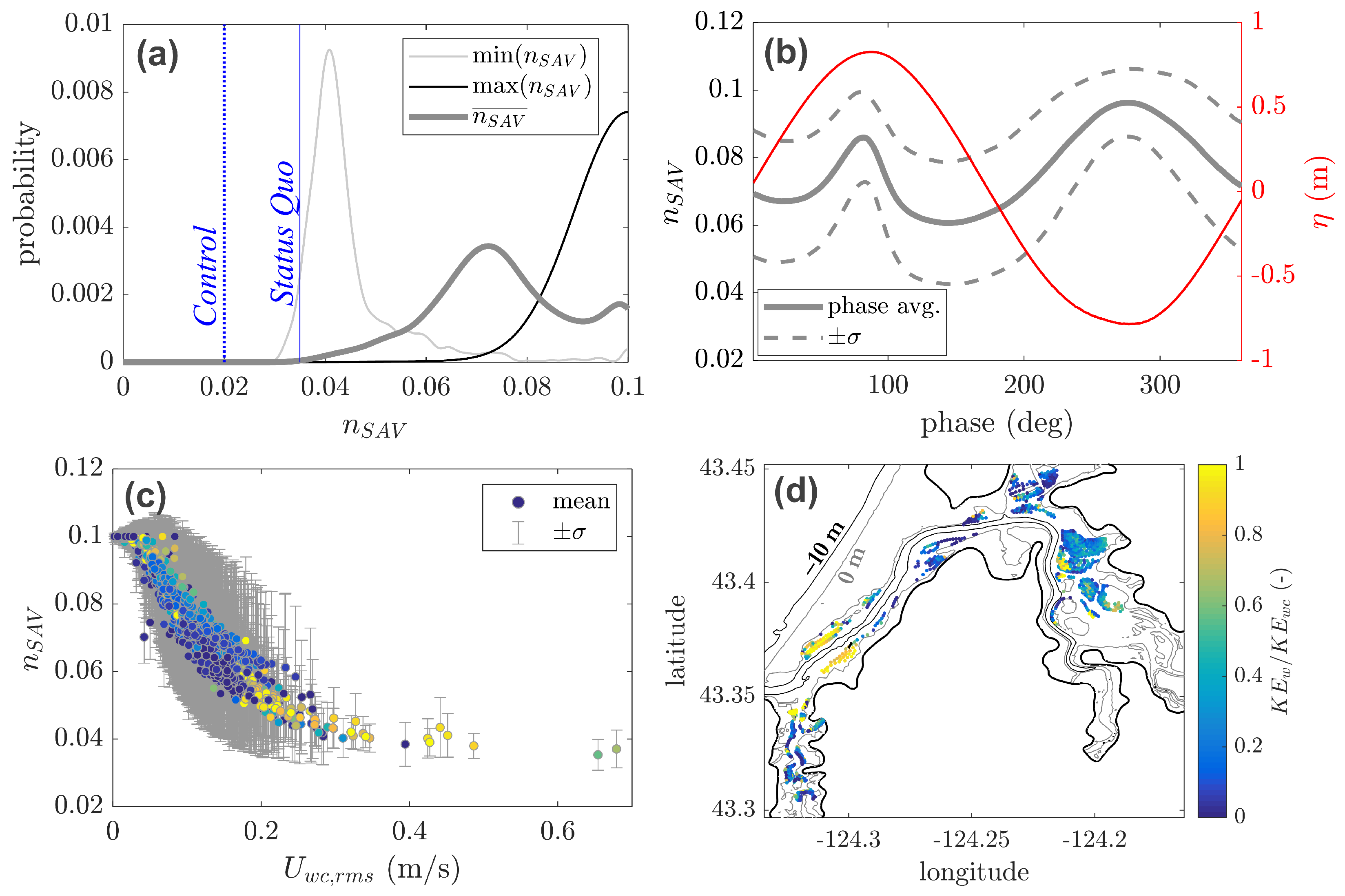
3.1. Characterization of Dynamic $n_{SAV}$

The inclusion of the dynamic Manning’s n routine results in temporal and spatial variation of the Manning’s n coefficient at the SAV nodes. As shown by the normalized probability distribution functions in Figure 3a, $n_{SAV}$ varied significantly across nodes. For each vegetated node, the value of $n_{SAV}$ varied over the model simulation between roughly 0.04 (mean minimum value) and 0.09 (mean maximum value). For comparison, blue dashed and solid lines at $n_{SAV}=$ 0.02 and 0.035, respectively, are included in Figure 3a to indicate commonly used values for open water (as used for the Control) and the SQ treatment, respectively (Section 2.5) [41,70,97,98].

A tidally phase-averaged value of $n_{SAV}$ was determined for each vegetated node by splitting the time series of the computed dynamic Manning’s n by tidal phase. When we then take the mean (across SAV nodes) phase-averaged $n_{SAV}$ and compare it with the phase-averaged water surface elevation $\eta$, we see that the two signals are well-correlated (Figure 3b). Values of $n_{SAV}$ are greatest when the tide stage is at extremes (low tide and high tide) and lowest during mid-tide when tidal current velocities are expected to be highest; the asymmetry in $n_{SAV}$ peak width during high and low tide closely matches the asymmetry in the phase-averaged tidal current magnitude (not shown). The strong dependence of $n_{SAV}$ on local flow velocities is further illustrated in Figure 3c, where the time-averaged mean and standard deviation $\sigma$ of $n_{SAV}$ for each vegetated node is shown to decrease with increasing $rms$ combined wave-current velocity $U_{wc,rms}$ [87]. Where $U_{wc,rms}$ is greater than approximately 0.2 m/s, the relative contribution of the waves to the total local velocity increases, which indicates that exclusion of waves from the simulation would underestimate the deflection of SAV and thus overestimate its dissipative capacity in areas where wave velocities are nontrivial (Figure 3d). In Figure 3c,d, the relative strength of the waves is represented as the wave kinetic energy fraction $K{E}_w/K{E}_{wc}$, which represents the ratio of kinetic energy (proportional to $U^2$) by waves alone $K{E}_w$ to the flow’s total kinetic energy by combined waves and currents $K{E}_{wc}$. Waves are said to dominate flow energy when values of $K{E}_w/K{E}_{wc}$ exceed approximately 0.75 [107].

3.2. Hydrodynamic and Sediment Transport Implications

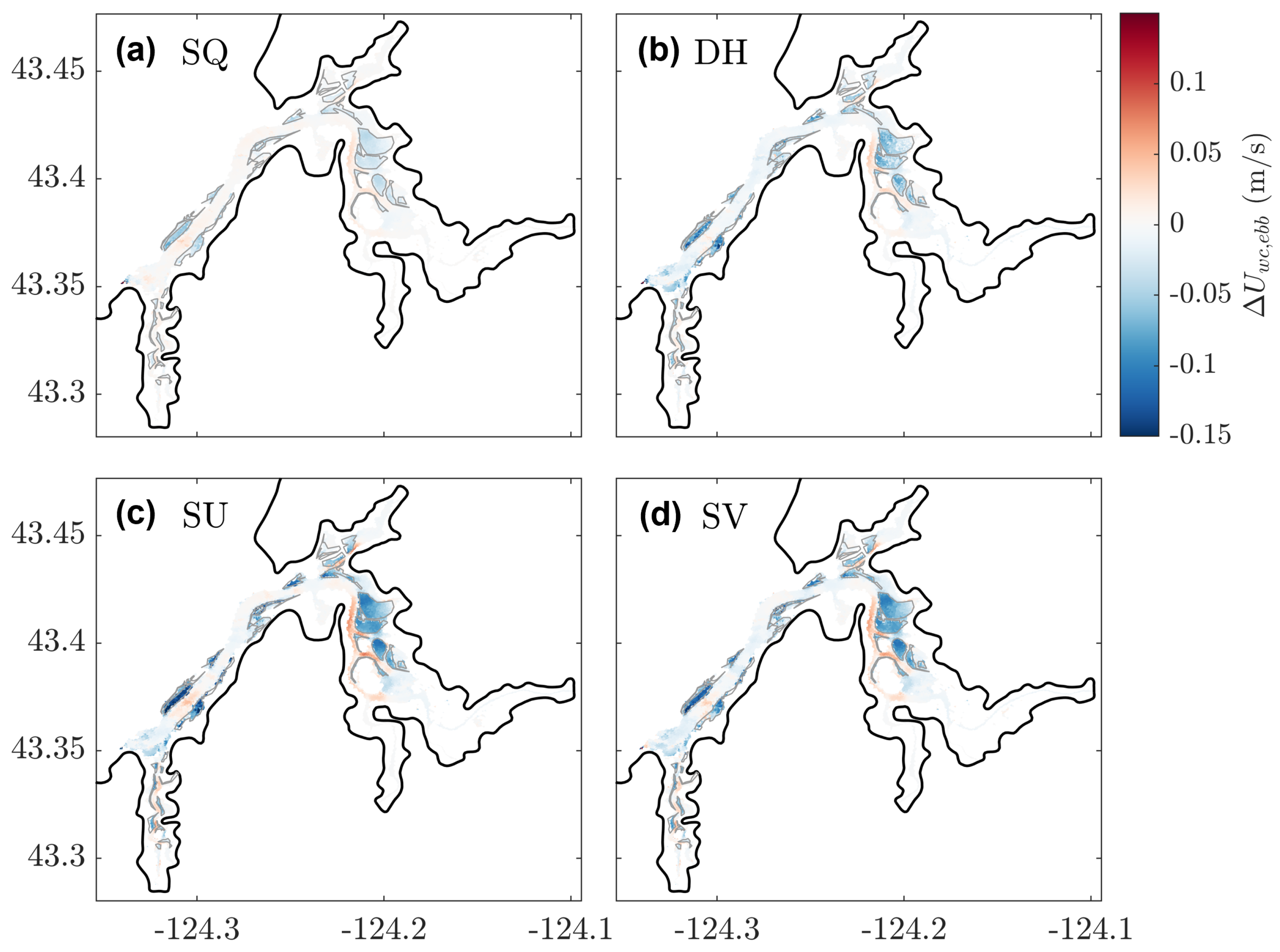
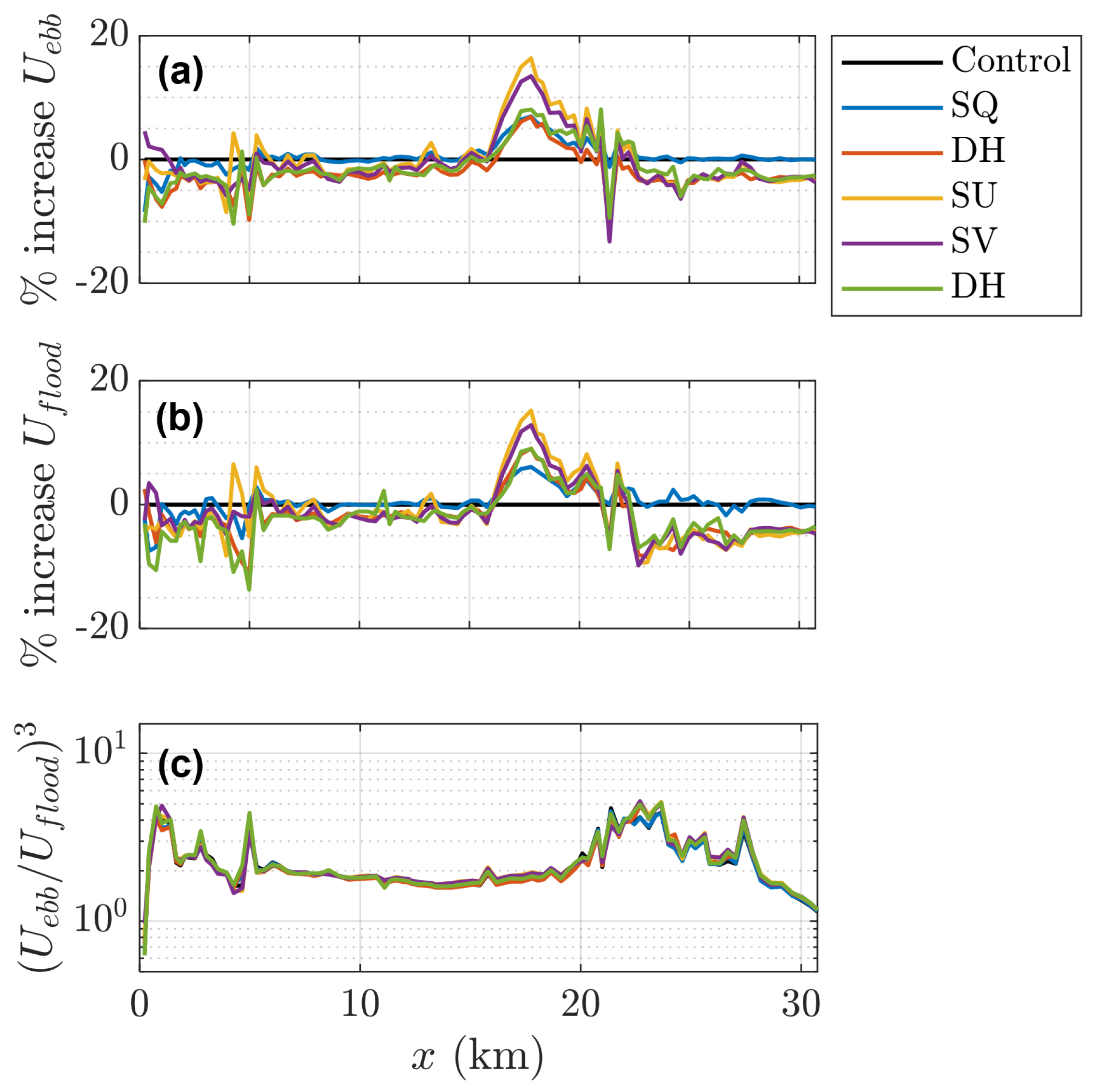
3.2.1. SAV Modification of Wave and Current Velocities

Spatial distributions of the change in combined wave-current velocities $\Delta U_{wc}$ during ebb tide due to the inclusion of SAV relative to the control are shown in Figure 4, where blues indicate a decrease in $U_{wc,ebb}$ when vegetation is included and reds indicate an increase. For all treatments, the characteristic $U_{wc,ebb}$, which is defined as the value of $U_{wc}$ averaged over instances of local minima in $d\eta /dt$ across all tidal cycles, is shown to decrease inside the areas designated as SAV habitats (outlined in grey) as compared to the control. As the value of $n_{SAV}$ used to parameterize SAV increases, reduction in $U_{wc,ebb}$ becomes larger. When large static values of $n_{SAV}$ are used (SU and SV, Figure 4c,d), distinct areas of increased $U_{wc,ebb}$ are seen in between SAV canopies. While this flow acceleration around canopies is shown for the SQ and DH cases (as well as DP, not shown), the funneling effect is less intense because values of $n_{SAV}$ for those treatments are much lower during peak ebb currents. When tidal velocities are at a maximum, $n_{SAV}$ is as low as 0.04 across much of the estuary for the dynamic treatments (DH and DP), which is very close to the static value of $n_{SAV}$ used for SQ treatment (0.035).

3.2.2. Sediment Fluxes

The change in total area of the sediment bed estimated to be mobilized (Equations (6)–(8)) due to the inclusion of SAV is shown in Figure 5. Inside SAV habitats, the greatest reduction in total area subject to sediment transport results from the SU treatment of SAV, and the smallest reduction results from the SQ treatment (Figure 5a). The DH, DP, and SV treatments reduced likelihood of sediment mobility inside SAV canopies relatively equally. Flow acceleration between SAV canopies during the high-Manning static treatments (SU and SV) is shown to increase the tendency for sediment motion in unvegetated regions of the CBE, as compared to the no-vegetation control, as well as compared to the DH and DP simulations (Figure 5b). In contrast, when SAV is allowed to deflect during the DH and DP treatments, $n_{SAV}$ is reduced during peak flows. The reduction in $n_{SAV}$ prevents excessive flow resistance that accelerates flow between patches and increases $\theta$ to above ${\theta }_c$ during the SU and SV treatments.

3.2.3. Circulation

In addition to quantifying SAV’s effect on localized hydrodynamics, we use a numerical drifter analysis to illustrate the cumulative impact of SAV on flow and circulation patterns in the CBE. Across the broad tidal flats flanking the main channel, numerical drifter pathlines are more narrowly concentrated in between SAV canopies when present (for all SAV treatment types), as opposed to a wider distribution of paths when SAV was not included in the model. Figure 6 shows the discretized pathlines of the drifters overlying elevation contours and SAV node locations in the CBE’s South Slough. The regions of the South Slough identified with arrows in Figure 6 demonstrate where SAV canopies can enhance or reroute dominant flow paths. As in the main channel, the presence of SAV along the deepest channel of South Slough narrows particle flow paths (denoted by solid grey arrow). For the DP simulation, SAV habitat in the southern-most tip of South Slough blocks the accumulation of drifters at the same location when SAV is absent during the Control and DH simulations (solid white arrow). The wider SAV coverage in the DP treatment also appears to trap particles outside of the main channel by creating low-velocity pockets (dashed arrows).

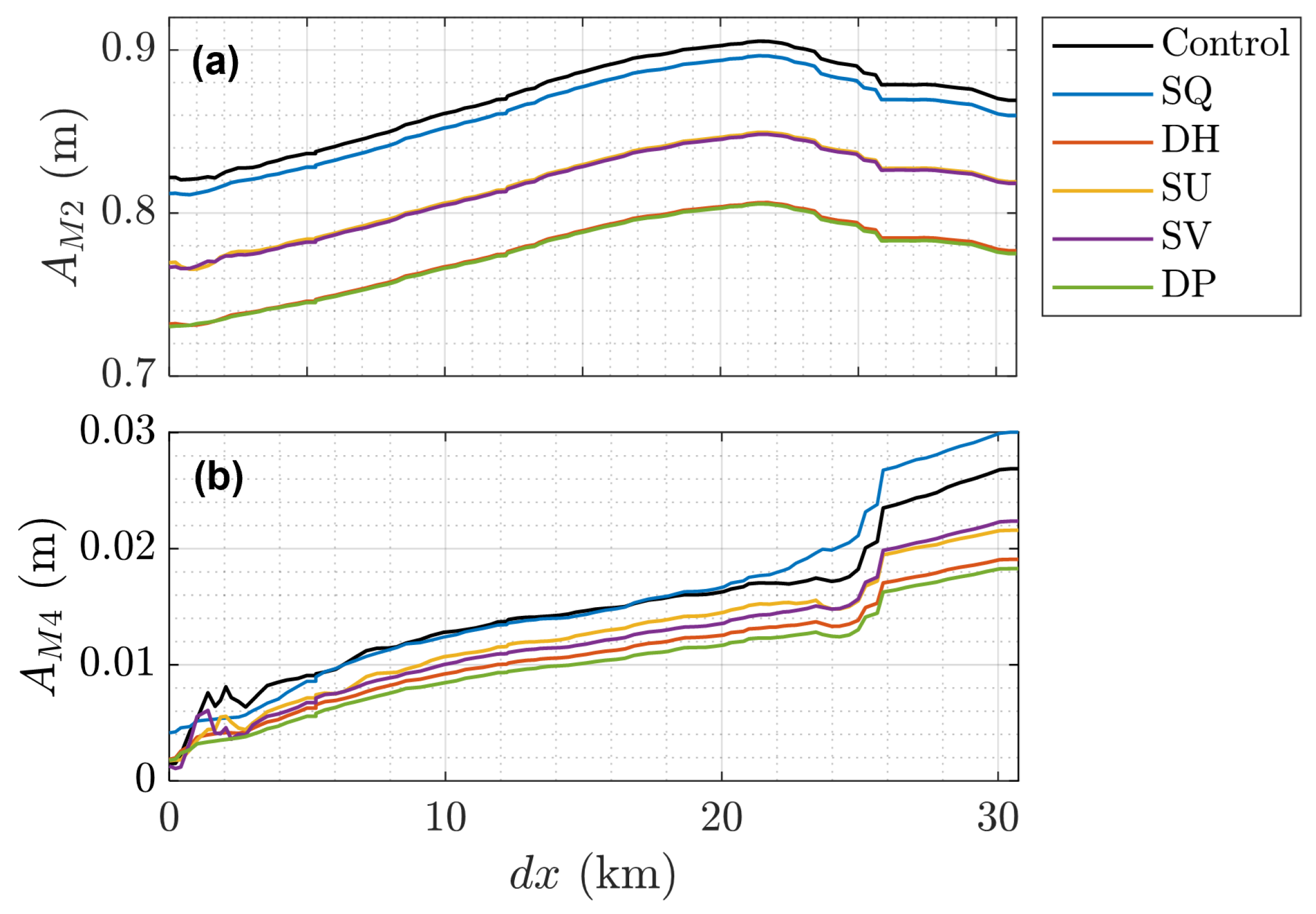
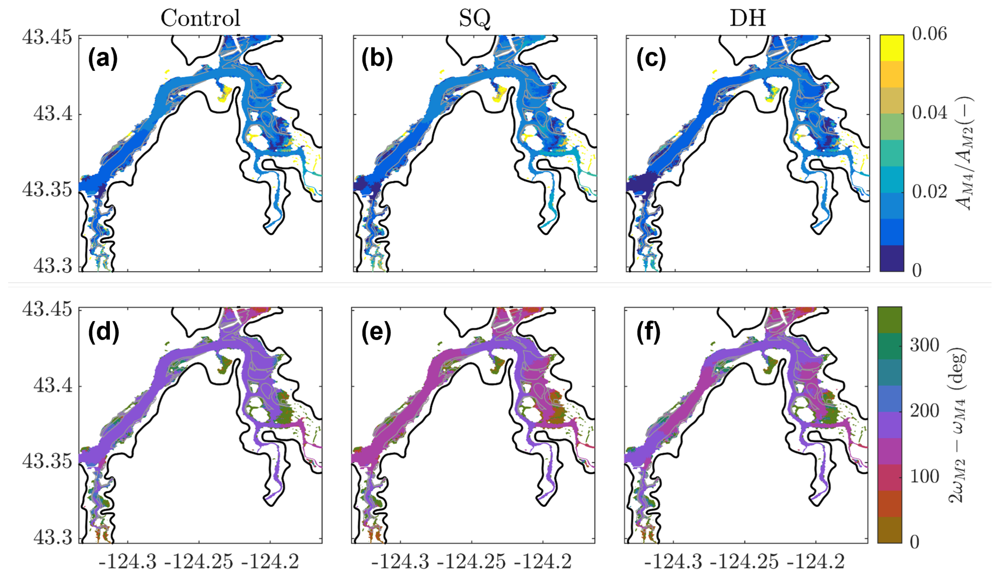
3.2.4. SAV Modification of Tidal Dynamics

The presence of SAV was shown to decrease the amplitude of the dominant tidal constituent $A_{M2}$ and its overtide $A_{M4}$ (Figure 7), for all SAV treatments excluding the SQ treatment. As shown in Figure 7a, the amplitude of the M2 constituent $A_{M2}$ was reduced by approximately the same amount for all along-channel distances $dx$; the DH and DP treatments reduced $A_{M2}$ by approximately 10 cm, while the reduction by the SV and SU treatments was slightly less at approximately 6 cm. Dissipation of the overtide M4 due to the presence of SAV increased with increasing $dx$ (Figure 7b). As with $A_{M2}$, the DH and DP treatments led to a larger reduction in $A_{M4}$ from the control. The SV and SU treatments also reduced $A_{M4}$ along the main channel. In contrast, the SQ case led to an increase in $A_{M4}$ for $dx$ greater than 20 km. Outside the main channel, reduction in $A_{M4}$ is further enhanced within SAV habitats.

Contours quantifying the relationship between the M2 and the M4 overtide are shown in Figure 8. The spatial variation in $A_{M4}$ dissipation shown in Figure 7b leads to spatial variability in the nonlinearity factor $A_{M4}/A_{M2}$ (Figure 8a–c). The presence of SAV appears to reduce $A_{M4}/A_{M2}$ relative to the control, especially within the first 5 km of the mouth of the CBE and in some of the shallowest portions of SAV habitats. The presence of SAV also led to a shift in the M2 constituent phase ${\omega }_{M2}$ and the M4 constituent phase ${\omega }_{M4}$. As compared to ${\omega }_{M2}$ for the control, the M2 tide arrives 87${}^{\circ }$ earlier for the SQ treatment, roughly 45${}^{\circ }$ later for the DH and DP treatments, and 10${}^{\circ }$–20${}^{\circ }$ later for the SU and SV treatments. Shifts in ${\omega }_{M2}$ were nearly uniform over the CBE. In contrast, shifts in ${\omega }_{M4}$ vary spatially over the domain; greater lags in ${\omega }_{M4}$ due to the presence of SAV are observed outside of SAV patches. The spatial variability in ${\omega }_{M4}$ due to SAV leads to spatial variability in 2${\omega }_{M2}-{\omega }_{M4}$ (Figure 8d–f). As with the $A_{M4}/A_{M2}$, the phase lag 2${\omega }_{M2}-{\omega }_{M4}$ is shown to decrease slightly within the first 5 km, indicating a slight potential for flood dominance within the first third of the main channel, as well as for the SAV-inhabited tidal flats on the eastern side of the main channel.

Following Eidam et al. [55], tidal ebb-flood dominance can also be determined by the cubed ratio of the average peak ebb velocity $U_{ebb}$ to the average peak flood velocity $U_{flood}$, where values greater than 1 indicate ebb dominance and values less than 1 indicate flood dominance. Values of $U_{ebb}^3/U_{flood}^3$ in Figure 9c are shown for nodes within the main channel with increasing distance $dx$ from the inlet. Although the presence of vegetation is shown to increase $U_{ebb}$ and $U_{flood}$ approximately 5–20% as compared to the control between $dx=$ 20–25 km (a and b, respectively), no significant change in $U_{ebb}^3/U_{flood}^3$ is observed in this section of the main channel. Excluding the region of $dx=$ 20–25 km, the presence of SAV is shown to slightly decrease $U_{ebb}$ and $U_{flood}$ for all treatments but the SQ treatment. Again, these slight modifications do not lead to an appreciable change in $U_{ebb}^3/U_{flood}^3$.

4. Discussion

The following subsections are organized thematically to provide a holistic overview of the impact of SAV and the dynamic friction routine on estuarine processes. Flexible SAV is shown to influence hydrodynamics across a range of scales in the CBE. We also discuss the applicability and limitations of our findings, as well as ecological parameter uncertainty.

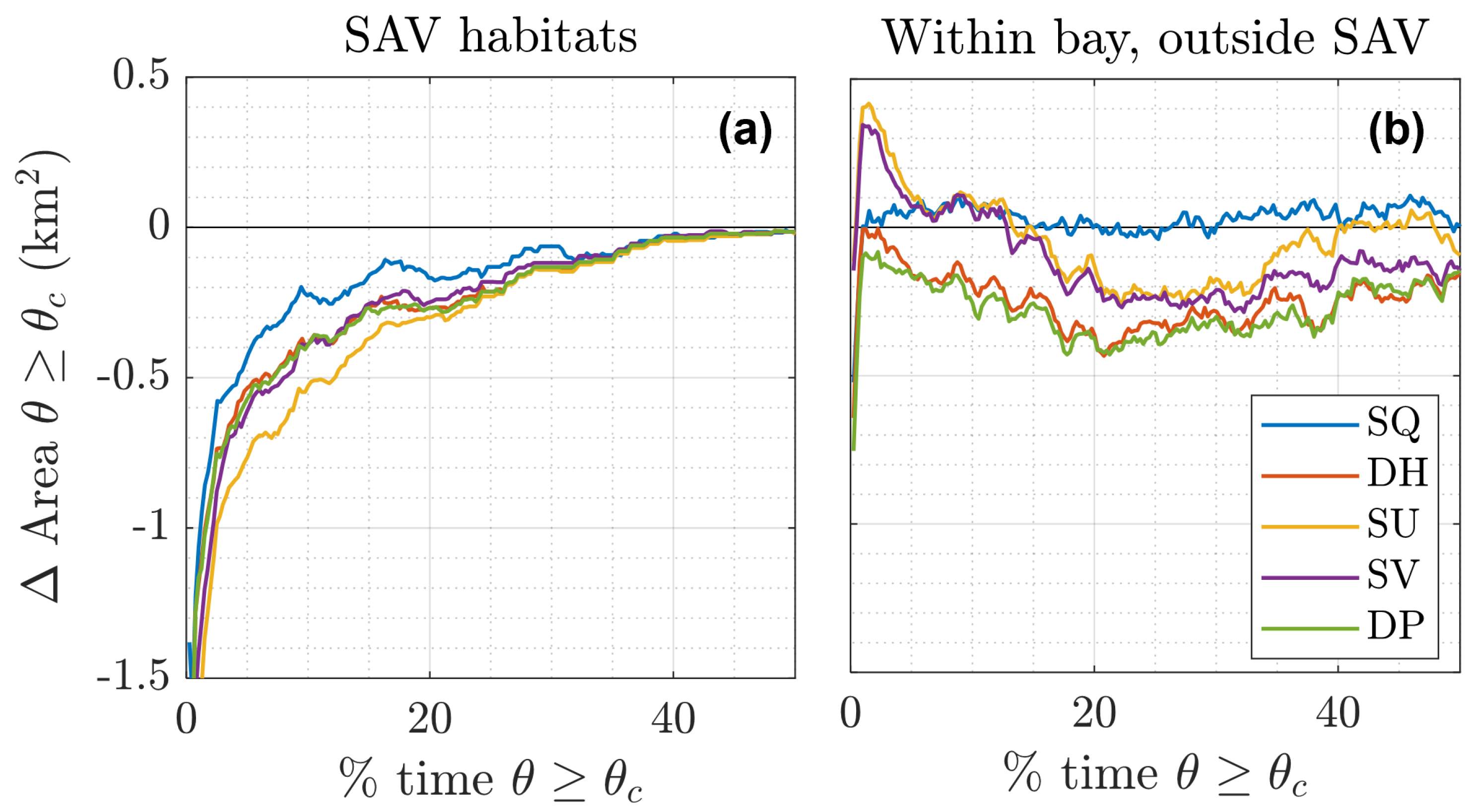
4.1. Spatial and Temporal Dependence of SAV Attenuation

Velocity reduction by SAV varies considerably throughout the CBE. Discontinuous SAV canopies significantly reduce combined wave-current velocities within the canopies themselves, but are shown to create a potential for flow acceleration and sediment mobility in bare areas neighboring and between canopies (Figure 4 and Figure 5). The variation in velocity attenuation is not only due to the discontinuity of SAV habitat, but also the spatial variability in hydrodynamics of the CBE. The horseshoe shape of the CBE, combined with strong riverine, wave, and wind forcing, results in a non-uniform distribution of $U_{wc,rms}$. The spatial and temporal variation in $U_{wc,rms}$ has important ramifications for accurate estimation of bottom friction by SAV because drag across flexible blades is limited by the intensity of local hydrodynamics. In areas where combined wave-current velocities are high, SAV deflection is also high, resulting in a reduction in $n_{SAV}$ (Figure 3c). Unlike static treatments, dynamic treatments of SAV bottom friction do not require a priori determination of $n_{SAV}$ for habitats across a spatially varying flow field. Furthermore, without including the influence of oceanic and wind waves on the total flow velocity, SAV deflection would be underestimated in unsheltered and near-mouth regions of the CBE (Figure 3d). Hydrodynamic patterns contribute to the spatial variability in velocity attenuation by SAV, and our results support the need for modeling both mean flow and wave statistics to accurately parameterize SAV-induced bottom friction in numerical models.

Because estuarine hydrodynamics additionally evolve on diurnal time scales, bottom friction by SAV also evolves temporally (Figure 3b). Time-varying SAV stem motion by naturally variable flow conditions necessitates the inclusion of dynamic deflection of SAV in numerical bottom friction routines. As shown in Figure 4, excluding SAV dynamics and assuming static behavior can overestimate flow dissipation within SAV canopies, increasing flow velocities adjacent to the canopies by as much as 5 cm/s. This overprediction of funneling around SAV habitats can overestimate the likelihood of sediment transport (Figure 5b). In compound estuaries like the CBE, variable streamflow rates, wave conditions, and wind fields additionally contribute to temporal variability in wave-current velocity fields. It is worth noting that there may be some contexts in which assuming temporal uniformity may be acceptable as long as the spatial variation remains. For example, flow attenuation and likelihood of sediment transport inside SAV canopies was shown to be nearly identical for the DH, DP, and SV treatments (Figure 5a).

4.2. Integrated Influence of SAV Attenuation

Particle tracking and tidal constituent analyses give an integrated view of flow attenuation by SAV across discontinuous habitats. As indicated in Figure 6, SAV meadows can lead to stalled flows outside the reach of the main channel. While not a precise metric of residence time, the apparent pooling of numerical drifters in sections of the CBE far from the main channel suggests that SAV can reduce flushing rates in already sheltered areas, which could be important for predicting system turbidity over time. More so than estuarine circulation, tidal amplitudes in particular were shown to be affected by both SAV presence and treatment type (Figure 7). Even in the main channel where depths and velocities are greatest, the M2 tidal constituent amplitude decreased by 8% for the SU and SV treatments and 11% for the DH and DP treatments; the same reduction in $A_{M2}$ by each treatment was observed uniformly across all areas of the CBE. Estuarine-scale changes in tidal constituent amplitudes decreased nonlinearity $A_{M4}/A_{M2}$ near the inlet and within SAV canopies, particularly so for the DH (and DP, not shown) treatments and less so for the SQ treatment (Figure 8). Interestingly, the SQ treatment led to the greatest increase in area where the phase relationship $2{\omega }_{M2}-{\omega }_{M4}$ decreased towards flood-dominant values. The ability of discontinuous SAV habitats to collectively shift tidal dynamics in the CBE towards flood dominance is consistent with findings by Donatelli et al. [22], meaning that time-averaged hydro- and sediment transport fluxes are directed into the estuary and potentially lead to increased sediment retention.

4.3. Relative Role of SAV in the CBE

While it has been shown that enhanced bottom friction dissipates ebb current velocities (enhanced by streamflow) more than flood current velocities (reduced by streamflow) [22], we note that this assumption does not necessarily hold for the case of flexible SAV that may deflect more under stronger ebb velocities than flood velocities. Furthermore, although SAV habitats across the CBE were shown to modify tidal constituents and peak current velocities (Figure 9a,b), the presence and treatment of SAV are not shown to definitively drive large changes in the ratio of modeled observations of ebb and flood velocities (Figure 9c). Thus, neither the presence nor the treatment of SAV appear to play a significant role in controlling ebb and flood dominance in the CBE. The minor role of SAV on the CBE’s peak current asymmetry contrasts with the strong influence by changes in estuarine bathymetry [55]. Eidam et al. [55] show that historical bathymetric changes (i.e., dredging of the main channel) have shifted the CBE from flood dominant to strongly ebb dominant. Finally, we note that the effect of SAV on the ratio of ebb and flood velocities is not expected to change under average seasonal streamflow variability. In JJA when streamflow is much lower, tidal duration asymmetry and peak velocity asymmetry are expected to be less [16]. If current velocities are less skewed, SAV deflection and, thus, SAV velocity attenuation, is likely to be fairly uniform under ebbing and flooding tidal periods. As under DJF streamflow conditions, dynamic treatments of SAV are likely to have a similar effect on peak current asymmetry as static treatments.

Despite the lack of significant change in peak current asymmetry by SAV, accretion of sediment within and on the shoreward edges of sheltered canopies (Figure 5 and Figure 6) may still result in net accumulation of material within the estuary even though sediment infilling by tides and mean currents is not expected. Treatment type (static vs. dynamic) may also influence the magnitude and spatial distribution of sediment retention, as static treatments are shown to enhance flow routing between canopies but more strongly reduce velocities within canopies (Figure 4).

4.4. Applicability to Other Systems

Seagrasses are found in sheltered, shallow coastal waters across the globe at all but polar latitudes [108,109]. Thus, our investigation into the large-scale control of SAV on hydrodynamics has widespread relevance for estuaries with similar levels of SAV coverage. In the CBE sensitivity study, each of our modeled canopies was between 0.1 and 1 km${}^2$, totaling nearly 8 km${}^2$ or 17% of the CBE’s total area below MSL. SAV presence may have a less significant influence on circulation and tidal dynamics in estuaries and embayments with less extensive coverage. From a management perspective, the restoration or loss of a singular canopy may not have significant impacts on regional dynamics, but large-scale die off events or habitat migration are more likely to impact tidal dynamics as well as the spatial distribution and frequency of sediment mobility. From a modeling perspective, a temporally varying dynamic friction routine may not be needed to capture the hydrodynamic impact of smaller habitats on large systems, such as in estuaries where total SAV habitat coverage is relatively small; values of $n_{SAV}$ may be nearly uniform across small, cohesive SAV canopies. However, a gradient in deflected stem height becomes more evident for larger SAV meadows due to the cascading effect of velocity and wave height attenuation with increasing distance into the meadow. Such spatial variation is also important to capture when modeling the localized hydrodynamics and sediment transport in and around vegetation canopies. As canopies and habitats become larger and/or increase in coverage over the hydrodynamic area of interest, the need for adaptive bottom friction treatments becomes greater.

Although not investigated in this study, variability in plant morphology should also be considered in site-specific parameterizations of bottom roughness by SAV, when known. In particular, SAV plant stem density has been shown to have the greatest control on its dissipative capacity [110]. Although variation in plant height $l_v$ for flexible species has little impact on its effective height $l_e$ and resulting dissipative capacity [110], increased plant stiffness (E and I) increases the sensitivity to $l_v$ uncertainty (Section 1.2). As E and I increase, the Cauchy number approaches zero, meaning plant deflection becomes negligible and stems remain static. In this study, modeled time-averaged values of $l_e$ are shown to be approximately half of $l_v$ throughout most of the estuary, excluding the near-inlet patches where time averaged $l_e/l_v$ is shown to be closer to 0.2 (co-located with $K{E}_w/K{E}_{wc}\sim 1$, Figure 3d). In very sheltered reaches of the estuary where $U_{wc,rms}\sim 0$ (Figure 3c), the friction routine is less sensitive to plant rigidity because $l_e$ is approximately equal to $l_v$ for the duration of the simulation. Using a bottom friction value representative of rigid vegetation would alter, but not eliminate, the time-varying nature of vegetation-induced bottom friction n because the formulation presented here is a function of plant submergence $l_e/h\left(t\right)$ [77]; for the same reason, values of n should also vary spatially for domains with spatially varying bathymetry. Thus, some form of adaptive friction routine should still be employed.

5. Conclusions

SAV species are ecologically valuable NNBFs in estuaries worldwide. Understanding how discontinuous SAV habitats control fluid and sediment transport pathways can be a critical component to planning and siting SAV restoration efforts. As numerical modelers move towards more physically representative parameterizations of SAV, we show that allowing for plant deflection is essential to realistically estimating the effect of flexible, buoyant SAV species on velocities within and adjacent to SAV habitats. Furthermore, estimating plant motion should account for wave-induced mean flow as well as tidally driven currents so as not to overestimate SAV drag forces during slack tide. In the Coos Bay Estuary investigated in this study, neglecting SAV deflection leads to over-attenuation of flow velocities within canopies and enhanced flow velocities in the unvegetated areas adjacent to the canopies. In the deep unvegetated main channel of the CBE, intertidal canopies of flexible SAV are also shown to dissipate tidal constituent energy more than, but reduce peak ebb and flood current velocities less than, static SAV treatments. This work demonstrates a valuable framework that can be utilized in any coupled wave-circulation numerical model to better account for sub-grid SAV canopy dynamics.

References

1. McLusky, D.; Elliott, M. The Estuarine Ecosystem: Ecology, Threats and Management; OUP Oxford: Oxford, UK, 2004. [Google Scholar]
2. Buschman, F.; Van Der Vegt, M.; Hoitink, A.; Hoekstra, P. Water and suspended sediment division at a stratified tidal junction. J. Geophys. Res. Ocean. 2013, 118, 1459–1472. [Google Scholar] [CrossRef] [Green Version]
3. Zhang, F.; Sun, J.; Lin, B.; Huang, G. Seasonal hydrodynamic interactions between tidal waves and river flows in the Yangtze Estuary. J. Mar. Syst. 2018, 186, 17–28. [Google Scholar] [CrossRef]
4. Bryan, K.R.; Nardin, W.; Mullarney, J.C.; Fagherazzi, S. The role of cross-shore tidal dynamics in controlling intertidal sediment exchange in mangroves in Cù Lao Dung, Vietnam. Cont. Shelf Res. 2017, 147, 128–143. [Google Scholar] [CrossRef]
5. Mazda, Y.; Wolanski, E.; King, B.; Sase, A.; Ohtsuka, D.; Magi, M. Drag force due to vegetation in mangrove swamps. Mangroves Salt Marshes 1997, 1, 193–199. [Google Scholar] [CrossRef]
6. Temmerman, S.; Bouma, T.J.; Govers, G.; Wang, Z.; De Vries, M.; Herman, P. Impact of vegetation on flow routing and sedimentation patterns: Three-dimensional modeling for a tidal marsh. J. Geophys. Res. Earth Surf. 2005, 110. [Google Scholar] [CrossRef]
7. Mazda, Y.; Kanazawa, N.; Wolanski, E. Tidal asymmetry in mangrove creeks. Hydrobiologia 1995, 295, 51–58. [Google Scholar] [CrossRef]
8. Nardin, W.; Larsen, L.; Fagherazzi, S.; Wiberg, P. Tradeoffs among hydrodynamics, sediment fluxes and vegetation community in the Virginia Coast Reserve, USA. Estuar. Coast. Shelf Sci. 2018, 210, 98–108. [Google Scholar] [CrossRef]
9. Savenije, H.H.; Toffolon, M.; Haas, J.; Veling, E.J. Analytical description of tidal dynamics in convergent estuaries. J. Geophys. Res. Ocean. 2008, 113, C10025. [Google Scholar] [CrossRef]
10. Cook, S.; Lippmann, T. Tidal Energy Dissipation in Three Estuarine Environments; Coastal Dynamics: San Juan, Trinidad and Tobago, 2017; pp. 346–355. [Google Scholar]
11. Du, J.; Shen, J.; Zhang, Y.J.; Ye, F.; Liu, Z.; Wang, Z.; Wang, Y.P.; Yu, X.; Sisson, M.; Wang, H.V. Tidal response to sea-level rise in different types of estuaries: The Importance of Length, Bathymetry, and Geometry. Geophys. Res. Lett. 2018, 45, 227–235. [Google Scholar] [CrossRef] [Green Version]
12. Speer, P.; Aubrey, D. A study of non-linear tidal propagation in shallow inlet/estuarine systems Part II: Theory. Estuar. Coast. Shelf Sci. 1985, 21, 207–224. [Google Scholar] [CrossRef]
13. Cook, S.E.; Lippmann, T.C.; Irish, J.D. Modeling nonlinear tidal evolution in an energetic estuary. Ocean Model. 2019, 136, 13–27. [Google Scholar] [CrossRef]
14. Nielsen, P. Coastal Bottom Boundary Layers and Sediment Transport; World Scientific: Singapore, 1992; Volume 4. [Google Scholar]
15. Wang, Z.; Jeuken, M.; Gerritsen, H.; De Vriend, H.; Kornman, B. Morphology and asymmetry of the vertical tide in the Westerschelde estuary. Cont. Shelf Res. 2002, 22, 2599–2609. [Google Scholar] [CrossRef]
16. Guo, L.; Wang, Z.B.; Townend, I.; He, Q. Quantification of tidal asymmetry and its nonstationary variations. J. Geophys. Res. Ocean. 2019, 124, 773–787. [Google Scholar] [CrossRef]
17. Ralston, D.K.; Talke, S.; Geyer, W.R.; Al-Zubaidi, H.A.; Sommerfield, C.K. Bigger tides, less flooding: Effects of dredging on barotropic dynamics in a highly modified estuary. J. Geophys. Res. Ocean. 2019, 124, 196–211. [Google Scholar] [CrossRef] [Green Version]
18. Horrevoets, A.; Savenije, H.; Schuurman, J.; Graas, S. The influence of river discharge on tidal damping in alluvial estuaries. J. Hydrol. 2004, 294, 213–228. [Google Scholar] [CrossRef]
19. Cai, H.; Savenije, H.; Toffolon, M. Linking the river to the estuary: Influence of river discharge on tidal damping. Hydrol. Earth Syst. Sci. 2014, 18, 287–304. [Google Scholar] [CrossRef] [Green Version]
20. Snyder, R.; Sidjabat, M.; Filloux, J. A study of tides, setup and bottom friction in a shallow semi-enclosed basin. Part II: Tidal model and comparison with data. J. Phys. Oceanogr. 1979, 9, 170–188. [Google Scholar] [CrossRef] [Green Version]
21. Georgas, N. Large seasonal modulation of tides due to ice cover friction in a midlatitude estuary. J. Phys. Oceanogr. 2012, 42, 352–369. [Google Scholar] [CrossRef] [Green Version]
22. Donatelli, C.; Ganju, N.K.; Kalra, T.S.; Fagherazzi, S.; Leonardi, N. Changes in hydrodynamics and wave energy as a result of seagrass decline along the shoreline of a microtidal back-barrier estuary. Adv. Water Resour. 2019, 128, 183–192. [Google Scholar] [CrossRef]
23. Bos, A.R.; Bouma, T.J.; de Kort, G.L.; van Katwijk, M.M. Ecosystem engineering by annual intertidal seagrass beds: Sediment accretion and modification. Estuar. Coast. Shelf Sci. 2007, 74, 344–348. [Google Scholar] [CrossRef]
24. Sherman, K.; DeBruyckere, L.A. Eelgrass Habitats on the U.S. West Coast: State of the Knowledge of Eelgrass Ecosystem Services and Eelgrass Extent; Technical Report; Pacific Marine and Estuarine Fish Habitat Partnership: Salem, OR, USA, 2018. [Google Scholar]
25. Thom, A. Momentum absorption by vegetation. Q. J. R. Meteorol. Soc. 1971, 97, 414–428. [Google Scholar] [CrossRef]
26. Luhar, M.; Nepf, H.M. From the blade scale to the reach scale: A characterization of aquatic vegetative drag. Adv. Water Resour. 2013, 51, 305–316. [Google Scholar] [CrossRef]
27. Beudin, A.; Kalra, T.S.; Ganju, N.K.; Warner, J.C. Development of a coupled wave-flow-vegetation interaction model. Comput. Geosci. 2017, 100, 76–86. [Google Scholar] [CrossRef]
28. Dalrymple, R.A.; Kirby, J.T.; Hwang, P.A. Wave diffraction due to areas of energy dissipation. J. Waterw. Port Coastal Ocean Eng. 1984, 110, 67–79. [Google Scholar] [CrossRef]
29. Mendez, F.J.; Losada, I.J. An empirical model to estimate the propagation of random breaking and nonbreaking waves over vegetation fields. Coast. Eng. 2004, 51, 103–118. [Google Scholar] [CrossRef]
30. Suzuki, T.; Zijlema, M.; Burger, B.; Meijer, M.C.; Narayan, S. Wave dissipation by vegetation with layer schematization in SWAN. Coast. Eng. 2012, 59, 64–71. [Google Scholar] [CrossRef]
31. Kobayashi, N.; Raichle, A.W.; Asano, T. Wave attenuation by vegetation. J. Waterw. Port Coast. Ocean Eng. 1993, 119, 30–48. [Google Scholar] [CrossRef]
32. Bradley, K.; Houser, C. Relative velocity of seagrass blades: Implications for wave attenuation in low-energy environments. J. Geophys. Res. Earth Surf. 2009, 114, F1. [Google Scholar] [CrossRef]
33. Anderson, M.; Smith, J. Wave attenuation by flexible, idealized salt marsh vegetation. Coast. Eng. 2014, 83, 82–92. [Google Scholar] [CrossRef]
34. Augustin, L.N.; Irish, J.L.; Lynett, P. Laboratory and numerical studies of wave damping by emergent and near-emergent wetland vegetation. Coast. Eng. 2009, 56, 332–340. [Google Scholar] [CrossRef]
35. Jadhav, R.S.; Chen, Q.; Smith, J.M. Spectral distribution of wave energy dissipation by salt marsh vegetation. Coast. Eng. 2013, 77, 99–107. [Google Scholar] [CrossRef] [Green Version]
36. Nepf, H.M. Drag, turbulence, and diffusion in flow through emergent vegetation. Water Resour. Res. 1999, 35, 479–489. [Google Scholar] [CrossRef]
37. Losada, I.J.; Maza, M.; Lara, J.L. A new formulation for vegetation-induced damping under combined waves and currents. Coast. Eng. 2016, 107, 1–13. [Google Scholar] [CrossRef]
38. Chen, H.; Ni, Y.; Li, Y.; Liu, F.; Ou, S.; Su, M.; Peng, Y.; Hu, Z.; Uijttewaal, W.; Suzuki, T. Deriving vegetation drag coefficients in combined wave-current flows by calibration and direct measurement methods. Adv. Water Resour. 2018, 122, 217–227. [Google Scholar] [CrossRef] [Green Version]
39. Wu, W.C.; Cox, D.T. Effects of wave steepness and relative water depth on wave attenuation by emergent vegetation. Estuar. Coast. Shelf Sci. 2015, 164, 443–450. [Google Scholar] [CrossRef]
40. Hu, K.; Chen, Q.; Wang, H. A numerical study of vegetation impact on reducing storm surge by wetlands in a semi-enclosed estuary. Coast. Eng. 2015, 95, 66–76. [Google Scholar] [CrossRef]
41. Bunya, S.; Dietrich, J.C.; Westerink, J.; Ebersole, B.; Smith, J.; Atkinson, J.; Jensen, R.; Resio, D.; Luettich, R.; Dawson, C.; et al. A high-resolution coupled riverine flow, tide, wind, wind wave, and storm surge model for southern Louisiana and Mississippi. Part I: Model development and validation. Mon. Weather Rev. 2010, 138, 345–377. [Google Scholar] [CrossRef] [Green Version]
42. Wiyono, R.U.A. Unstructured Mesh Tsunami Simulation Using FVCOM Considering the Fine Structure of Land Use. Ph.D. Thesis, Yokohama National University, Yokohama, Kanagawa, 2015. [Google Scholar]
43. Nardin, W.; Locatelli, S.; Pasquarella, V.; Rulli, M.C.; Woodcock, C.E.; Fagherazzi, S. Dynamics of a fringe mangrove forest detected by Landsat images in the Mekong River Delta, Vietnam. Earth Surf. Process. Landf. 2016, 41, 2024–2037. [Google Scholar] [CrossRef]
44. Nardin, W.; Lera, S.; Nienhuis, J. Effect of offshore waves and vegetation on the sediment budget in the Virginia Coast Reserve (VA). Earth Surf. Process. Landf. 2020, 45, 3055–3068. [Google Scholar] [CrossRef]
45. Bandhoe, S. Modelling Interspecific Competition between the Salicornia and Spartina Species and Its Effect on the Bio-Geomorphological Development of Salt Marshes. Master’s Thesis, University of Twente, Enschede, The Netherlands, 2020. [Google Scholar]
46. Medeiros, S.C.; Hagen, S.C.; Weishampel, J.F. Comparison of floodplain surface roughness parameters derived from land cover data and field measurements. J. Hydrol. 2012, 452, 139–149. [Google Scholar] [CrossRef]
47. Kerr, P.; Martyr, R.; Donahue, A.; Hope, M.; Westerink, J.; Luettich, R., Jr.; Kennedy, A.; Dietrich, J.; Dawson, C.; Westerink, H. US IOOS coastal and ocean modeling testbed: Evaluation of tide, wave, and hurricane surge response sensitivities to mesh resolution and friction in the Gulf of Mexico. J. Geophys. Res. Ocean. 2013, 118, 4633–4661. [Google Scholar] [CrossRef]
48. Passeri, D.; Hagen, S.C.; Smar, D.; Alimohammadi, N.; Risner, A.; White, R. Sensitivity of an ADCIRC tide and storm surge model to Manning’s n. Estuar. Coast. Model. 2011, 2013, 457–475. [Google Scholar]
49. Abdolahpour, M.; Hambleton, M.; Ghisalberti, M. The wave-driven current in coastal canopies. J. Geophys. Res. Ocean. 2017, 122, 3660–3674. [Google Scholar] [CrossRef]
50. Lei, J.; Nepf, H. Blade dynamics in combined waves and current. J. Fluids Struct. 2019, 87, 137–149. [Google Scholar] [CrossRef]
51. van Veelen, T.J.; Fairchild, T.P.; Reeve, D.E.; Karunarathna, H. Experimental study on vegetation flexibility as control parameter for wave damping and velocity structure. Coast. Eng. 2020, 157, 103648. [Google Scholar] [CrossRef]
52. Ashall, L.M.; Mulligan, R.P.; van Proosdij, D.; Poirier, E. Application and validation of a three-dimensional hydrodynamic model of a macrotidal salt marsh. Coast. Eng. 2016, 114, 35–46. [Google Scholar] [CrossRef]
53. Fringer, O.B.; Dawson, C.N.; He, R.; Ralston, D.K.; Zhang, Y.J. The future of coastal and estuarine modeling: Findings from a workshop. Ocean Model. 2019, 143, 101458. [Google Scholar] [CrossRef]
54. Rumrill, S. The Ecology of the South Slough Estuary: Site Profile of the South Slough National Estuarine Research Reserve; Technical Report; Oregon Department of State Lands: Salem, OR, USA, 2006.
55. Eidam, E.; Sutherland, D.; Ralston, D.; Dye, B.; Conroy, T.; Schmitt, J.; Ruggiero, P.; Wood, J. Impacts of 150 years of shoreline and bathymetric change in the Coos Estuary, Oregon, USA. Estuar. Coasts 2020, 1–19. [Google Scholar] [CrossRef]
56. Caldera, M. South Slough Adventures: Life on a Southern Oregon Estuary; South Coast Printing: Coos Bay, OR, USA, 1995. [Google Scholar]
57. Eidam, E.; Sutherland, D.; Ralston, D.; Conroy, T.; Dye, B. Shifting sediment dynamics in the Coos Bay Estuary in response to 150 years of modification. J. Geophys. Res. Ocean. 2021, 126, e2020JC016771. [Google Scholar] [CrossRef]
58. Hickey, B.M.; Banas, N.S. Oceanography of the US Pacific Northwest coastal ocean and estuaries with application to coastal ecology. Estuaries 2003, 26, 1010–1031. [Google Scholar] [CrossRef]
59. Engle, J.M.; Miller, K. Distribution and morphology of eelgrass (Zostera marina L.) at the California Channel Islands. In Proceedings of the Sixth California Islands Symposium, Arcata, CA, USA, 7–11 November 2005; pp. 405–414. [Google Scholar]
60. Parker, K.; Hill, D.; García-Medina, G.; Beamer, J. The effects of changing climate on estuarine water levels: A United States Pacific Northwest case study. Nat. Hazards Earth Syst. Sci. 2019, 19, 1601–1618. [Google Scholar] [CrossRef] [Green Version]
61. Henry Lee, I.; Brown, C.A. Classification of Regional Patterns of Environmental Drivers and Benthic Habitats in Pacific Northwest Estuaries; Technical Report; US Environmental Protection Agency: Washington, DC, USA, 2009.
62. Conroy, T.; Sutherland, D.A.; Ralston, D.K. Estuarine exchange flow variability in a seasonal, segmented estuary. J. Phys. Oceanogr. 2020, 50, 595–613. [Google Scholar] [CrossRef]
63. Risley, J.; Stonewall, A.; Haluska, T. Estimating Flow-Duration and Low-Flow Frequency Statistics for Unregulated Streams in Oregon; Technical Report; U.S. Geological Survey: Washington, DC, USA, 2008.
64. The StreamStats Program for Oregon. Available online: http://water.usgs.gov/osw/streamstats/colorado.html (accessed on 1 January 2020).
65. National Weather Service. U.S. States and Territories. Available online: http://www.nws.noaa.gov/geodata/catalog/national/html/us_state.htm (accessed on 1 January 2022).
66. Luettich, R.A.; Westerink, J.J.; Scheffner, N.W. ADCIRC: An Advanced Three-Dimensional Circulation Model for Shelves, Coasts, and Estuaries. Report 1, Theory and Methodology of ADCIRC-2DD1 and ADCIRC-3DL; Technical Report; US Army Engineer Waterways Experiment Station: Washington, DC, USA, 1992.
67. Dietrich, J.; Westerink, J.; Kennedy, A.; Smith, J.; Jensen, R.; Zijlema, M.; Holthuijsen, L.; Dawson, C.; Luettich, R.; Powell, M.; et al. Hurricane Gustav (2008) waves and storm surge: Hindcast, synoptic analysis, and validation in southern Louisiana. Mon. Weather Rev. 2011, 139, 2488–2522. [Google Scholar] [CrossRef]
68. Cheng, T.; Hill, D.; Read, W. The contributions to storm tides in Pacific northwest estuaries: Tillamook Bay, Oregon, and the December 2007 storm. J. Coast. Res. 2015, 31, 723–734. [Google Scholar] [CrossRef]
69. Graham, L.; Butler, T.; Walsh, S.; Dawson, C.; Westerink, J.J. A measure-theoretic algorithm for estimating bottom friction in a coastal inlet: Case study of bay St. Louis during hurricane Gustav (2008). Mon. Weather Rev. 2017, 145, 929–954. [Google Scholar] [CrossRef]
70. Garzon, J.L.; Ferreira, C.M. Storm surge modeling in large estuaries: Sensitivity analyses to parameters and physical processes in the Chesapeake Bay. J. Mar. Sci. Eng. 2016, 4, 45. [Google Scholar] [CrossRef] [Green Version]
71. Akbar, M.K.; Kanjanda, S.; Musinguzi, A. Effect of bottom friction, wind drag coefficient, and meteorological forcing in hindcast of Hurricane Rita storm surge using SWAN+ ADCIRC model. J. Mar. Sci. Eng. 2017, 5, 38. [Google Scholar] [CrossRef] [Green Version]
72. Egbert, G.D.; Erofeeva, S.Y. Efficient inverse modeling of barotropic ocean tides. J. Atmos. Ocean. Technol. 2002, 19, 183–204. [Google Scholar] [CrossRef] [Green Version]
73. Roberts, K.J.; Pringle, W.J.; Westerink, J.J. OceanMesh2D 1.0: MATLAB-based software for two-dimensional unstructured mesh generation in coastal ocean modeling. Geosci. Model Dev. 2019, 12, 1847–1868. [Google Scholar] [CrossRef] [Green Version]
74. Iowa State University Iowa Environmental Mesonet. Available online: https://mesonet.agron.iastate.edu/sites/site.php?station=OTH&network=OR_ASOS (accessed on 1 May 2021).
75. RAWS USA Climate Archive. Available online: https://raws.dri.edu/ (accessed on 1 May 2021).
76. Kalnay, E.; Kanamitsu, M.; Kistler, R.; Collins, W.; Deaven, D.; Gandin, L.; Iredell, M.; Saha, S.; White, G.; Woollen, J.; et al. The NCEP/NCAR 40-year reanalysis project. Bull. Am. Meteorol. Soc. 1996, 77, 437–472. [Google Scholar] [CrossRef] [Green Version]
77. Baptist, M.; Babovic, V.; Rodríguez Uthurburu, J.; Keijzer, M.; Uittenbogaard, R.; Mynett, A.; Verwey, A. On inducing equations for vegetation resistance. J. Hydraul. Res. 2007, 45, 435–450. [Google Scholar] [CrossRef]
78. Uittenbogaard, R. Modelling turbulence in vegetated aquatic flows. In Proceedings of the Riparian Forest Vegetated Channels Workshop, Trendo, Italy, 20–22 February 2003. [Google Scholar]
79. Luhar, M.; Nepf, H.M. Flow-induced reconfiguration of buoyant and flexible aquatic vegetation. Limnol. Oceanogr. 2011, 56, 2003–2017. [Google Scholar] [CrossRef] [Green Version]
80. Philips, R.C. The Ecology of Eelgrass Meadows in the Pacific Northwest: A Community Profile; Technical Report; US Fish and Wildflife Service: Washington, DC, USA, 1984.
81. Gambi, M.C.; Nowell, A.R.; Jumars, P.A. Flume observations on flow dynamics in Zostera marina (eelgrass) beds. Mar. Ecol. Prog. Ser. 1990, 61, 159–169. [Google Scholar] [CrossRef]
82. Thom, R.M.; Borde, A.B.; Rumrill, S.; Woodruff, D.L.; Williams, G.D.; Southard, J.A.; Sargeant, S.L. Factors influencing spatial and annual variability in eelgrass (Zostera marina L.) meadows in Willapa Bay, Washington, and Coos Bay, Oregon, estuaries. Estuaries 2003, 26, 1117–1129. [Google Scholar] [CrossRef]
83. Lefebvre, A.; Thompson, C.; Amos, C. Influence of Zostera marina canopies on unidirectional flow, hydraulic roughness and sediment movement. Cont. Shelf Res. 2010, 30, 1783–1794. [Google Scholar] [CrossRef]
84. Abdelrhman, M.A. Modeling coupling between eelgrass Zostera marina and water flow. Mar. Ecol. Prog. Ser. 2007, 338, 81–96. [Google Scholar] [CrossRef] [Green Version]
85. Ruessink, B.G.; Michallet, H.; Abreu, T.; Sancho, F.; Van Der A, D.A.; Van Der Werf, J.J.; Silva, P.A. Observations of velocities, sand concentrations, and fluxes under velocity-asymmetric oscillatory flows. J. Geophys. Res. Ocean. 2011, 116, C3. [Google Scholar] [CrossRef] [Green Version]
86. Hessing-Lewis, M.L.; Hacker, S.D.; Menge, B.A.; Rumrill, S.S. Context-dependent eelgrass–macroalgae interactions along an estuarine gradient in the Pacific Northwest, USA. Estuar. Coasts 2011, 34, 1169–1181. [Google Scholar] [CrossRef]
87. Lacy, J.R.; Rubin, D.M.; Ikeda, H.; Mokudai, K.; Hanes, D.M. Bed forms created by simulated waves and currents in a large flume. J. Geophys. Res. Ocean. 2007, 112, C10. [Google Scholar] [CrossRef] [Green Version]
88. Luhar, M.; Infantes, E.; Orfila, A.; Terrados, J.; Nepf, H.M. Field observations of wave-induced streaming through a submerged seagrass (Posidonia oceanica) meadow. J. Geophys. Res. Ocean. 2013, 118, 1955–1968. [Google Scholar] [CrossRef] [Green Version]
89. Chow, V.T. Open Channel Hydraulics; McGraw Hill: New York, NY, USA, 1959. [Google Scholar]
90. Bretschneider, C.L.; Agrawal, J.D.; Carmella, N.C.; Wohlmut, K.A. Hurricane Iniki, hindcast, winds, windwaves, swells, storm surge, and wave runup. In Proceedings of the American Society of Civil Engineers, Hurricanes of 1992 Technical Conference, Miami, FL, USA, 1–3 December 1993. [Google Scholar]
91. Madsen, O.S.; Poon, Y.K.; Graber, H.C. Spectral wave attenuation by bottom friction: Theory. In Proceedings of the 21st International Conference on Coastal Engineering, Costa del Sol-Malaga, Spain, 20–25 June 1988; pp. 492–504. [Google Scholar]
92. Baron-Hyppolite, C.; Lashley, C.H.; Garzon, J.; Miesse, T.; Ferreira, C.; Bricker, J.D. Comparison of Implicit and Explicit Vegetation Representations in SWAN Hindcasting Wave Dissipation by Coastal Wetlands in Chesapeake Bay. Geosciences 2019, 9, 8. [Google Scholar] [CrossRef] [Green Version]
93. Moki, H.; Taguchi, K.; Nakagawa, Y.; Montani, S.; Kuwae, T. Spatial and seasonal impacts of submerged aquatic vegetation (SAV) drag force on hydrodynamics in shallow waters. J. Mar. Syst. 2020, 209, 103373. [Google Scholar] [CrossRef]
94. Zhao, H.; Chen, Q. Modeling attenuation of storm surge over deformable vegetation: Parametric study. J. Eng. Mech. 2016, 142, 06016006. [Google Scholar] [CrossRef]
95. Zhao, H.; Chen, Q. Modeling attenuation of storm surge over deformable vegetation: Methodology and verification. J. Eng. Mech. 2014, 140, 04014090. [Google Scholar] [CrossRef]
96. Wickham, J.; Stehman, S.V.; Sorenson, D.G.; Gass, L.; Dewitz, J.A. Thematic accuracy assessment of the NLCD 2016 land cover for the conterminous United States. Remote Sens. Environ. 2021, 257, 112357. [Google Scholar] [CrossRef]
97. Stark, J.; Plancke, Y.; Ides, S.; Meire, P.; Temmerman, S. Coastal flood protection by a combined nature-based and engineering approach: Modeling the effects of marsh geometry and surrounding dikes. Estuar. Coast. Shelf Sci. 2016, 175, 34–45. [Google Scholar] [CrossRef]
98. Paquier, A.E.; Oudart, T.; Le Bouteiller, C.; Meulé, S.; Larroudé, P.; Dalrymple, R.A. 3D numerical simulation of seagrass movement under waves and currents with GPUSPH. Int. J. Sediment Res. 2020, 36, 711–722. [Google Scholar] [CrossRef]
99. Soulsby, R. Dynamics of Marine Sands; T. Telford: London, UK, 1997. [Google Scholar]
100. Masselink, G.H.M.; Knight, J. Introduction to Coastal Processes and Geomorphology; Taylor and Francis: London, UK, 2011. [Google Scholar]
101. Edinger, J.E.; Buchak, E.M.; Kollubru, V.S. Modeling flushing and mixing in a deep estuary. Water Air Soil Pollut. 1998, 102, 345–353. [Google Scholar] [CrossRef]
102. Wang, C.F.; Hsu, M.H.; Kuo, A.Y. Residence time of the Danshuei River estuary, Taiwan. Estuar. Coast. Shelf Sci. 2004, 60, 381–393. [Google Scholar] [CrossRef]
103. Xu, D.; Xue, H.; Greenberg, D.A. A numerical study of the circulation and drifter trajectories in Cobscook Bay. Estuar. Coast. Model. 2005, 2006, 176–195. [Google Scholar]
104. Hill, D.; Ciavola, S.; Etherington, L.; Klaar, M. Estimation of freshwater runoff into Glacier Bay, Alaska and incorporation into a tidal circulation model. Estuar. Coast. Shelf Sci. 2009, 82, 95–107. [Google Scholar] [CrossRef]
105. Haase, A.T.; Eggleston, D.B.; Luettich, R.A.; Weaver, R.J.; Puckett, B.J. Estuarine circulation and predicted oyster larval dispersal among a network of reserves. Estuar. Coast. Shelf Sci. 2012, 101, 33–43. [Google Scholar] [CrossRef]
106. Hofmann, E.E.; Hedström, K.S.; Moisan, J.R.; Haidvogel, D.B.; Mackas, D.L. Use of simulated drifter tracks to investigate general transport patterns and residence times in the Coastal Transition Zone. J. Geophys. Res. Ocean. 1991, 96, 15041–15052. [Google Scholar] [CrossRef]
107. Wengrove, M.E.; Foster, D.L.; Lippmann, T.C.; de Schipper, M.A.; Calantoni, J. Observations of Bedform Migration and Bedload Sediment Transport in Combined Wave-Current Flows. J. Geophys. Res. Ocean. 2019, 124, 4572–4590. [Google Scholar] [CrossRef] [Green Version]
108. Short, F.T.; Coles, R.G. (Eds.) Global Seagrass Research Methods; Elsevier: Amsterdam, The Netherlands, 2001. [Google Scholar]
109. Orth, R.J.; Carruthers, T.J.B.; Dennison, W.C.; Duarte, C.M.; Fourqurean, J.W.; Heck, K.L.; Hughes, A.R.; Kendrick, G.A.; Kenworthy, W.J.; Olyarnik, S.; et al. A Global Crisis for Seagrass Ecosystems. BioScience 2006, 56, 987–996. [Google Scholar] [CrossRef] [Green Version]
110. Kalra, T.S.; Aretxabaleta, A.; Seshadri, P.; Ganju, N.K.; Beudin, A. Sensitivity analysis of a coupled hydrodynamic-vegetation model using the effectively subsampled quadratures method (ESQM v5. 2). Geosci. Model Dev. 2017, 10, 4511–4523. [Google Scholar] [CrossRef] [Green Version]
Figure 2. Dynamic bottom friction routine embedded into both ADCIRC and SWAN to capture vegetation deflection.
Jmse 10 00554 g002
Figure 3. Characterization of the dynamic bottom roughness coefficient for SAV, n S A V . (a) Comparison in the temporal mean, minimum, and maximum values of n S A V taken across all of the vegetated nodes. (b) Phase-averaged n S A V as a function of tidal phase, compared to the phase-averaged η . (c) Average mean and standard deviation of n S A V for each dynamic SAV node as a function of r m s combined wave and current velocity ( U w c , r m s ) and wave kinetic energy fraction ( K E w / K E w c ). (d) Spatial distribution of average K E w / K E w c at SAV nodes. Contours correspond to an elevation of 0 m (thin grey line) and −10 m (thin black line).
Jmse 10 00554 g003
Figure 4. Change in combined wave-current velocity during peak ebb currents U w c , e b b by SAV parameterized as (a) SQ, (b) DH, (c) SU, and (d) SV, as compared to no-vegetation control. Horizontal and vertical axes correspond to longitude and latitude (degrees).
Jmse 10 00554 g004
Figure 5. Change in total area where erosion threshold exceeded due to the inclusion of SAV via the tested SAV treatment as compared to control; x-axis corresponds to frequency of threshold exceedance (percent of 40-day simulation). Total within-bay area examined separately as area (a) outside SAV patches and (b) within SAV patches.
Jmse 10 00554 g005
Figure 6. Discretized numerical drifter pathlines (blue transparent) for simulations in which SAV is parameterized as (a) absent for the Control, (b) DH, and (c) DP. Location of SAV computational nodes shown in magenta. Elevation contours correspond to 0 m (thing grey line) and −5 m (thin black line). Arrows used as reference points in text. Bold black line indicates model boundary. Horizontal and vertical axes correspond to longitude and latitude (degrees).
Jmse 10 00554 g006
Figure 7. Change in tidal constituent amplitude for (a) M2 and (b) M4 as a function of along-channel distance from inlet d x (see Figure 1) for distance markers.
Jmse 10 00554 g007
Figure 8. (ac) Tidal asymmetry A M 4 / A M 2 and (df) phase difference 2 θ M 2 θ M 4 across CBE, where values greater than 180 indicate ebb dominance and values less than 180 indicate flood dominance. Horizontal and vertical axes correspond to longitude and latitude (degrees).
Jmse 10 00554 g008
Figure 9. Percent increase in average streamwise velocity during (a) peak ebb tide U e b b and (b) peak flood tide U f l o o d from the control as a function of distance up the main channel from inlet d x (Figure 1). (c) Cubed ratio of U e b b / U f l o o d as a function of d x .
Jmse 10 00554 g009