Effects of the Parameter C_4ε in the Extended k-ε Turbulence Model for Wind Farm Wake Simulation Using an Actuator Disc

Abstract

The actuator disc model (ADM) incorporated into the k-ε turbulence model of EI Kasmi is able to simulate the wind farm wakes with high fidelity, which is essential for layout optimization and the evaluation of power production in modern wind farms. However, the effects of the parameter C_4ε in the k-ε model of EI Kasmi on turbulent kinetic energy (TKE) in the superposition areas and the recovery of wind farm wake velocity have rarely been studied. To this end, the k-ε model of EI Kasmi is coupled with the advanced ADM in PHOENICS to investigate the influence of the parameter C_4ε on the wake simulation of wind farms (e.g., two offshore wind farms, one onshore wind farm). It is concluded that a decreased parameter C_4ε makes the generation range of TKE in the vicinity of the rotor smaller, but the TKE near the rotor becomes larger, and the wake recovery rate of the downstream turbine is less affected by the near wake. As the interwind turbine spacing increases, the influence area of TKE in the wake region of each downstream machine gradually reduces, and atmospheric turbulence plays a dominant role in wake recovery. A decreased parameter C_4ε can effectively promote the inflow wind velocity and power output of downstream turbines. The power output simulated compares well with the measured power value when the parameter C_4ε = 0.15.

1. Introduction

For a modern wind farm, wind turbines operating downwind may be located in the interaction of multiple wakes, which can bring about annual power deficits of 10% to 20% [1]. In addition, the complex turbulence interaction from more than two turbines endangers the lifespan of wind turbines, due to the limited spacing between the adjacent rotors. Hence, research on wake prediction modeling of wind farms is critical in the design phase for layout optimization [2] and micro-siting [3] in wind farms.

Wind farm wake modeling methodologies are mainly divided into analytical wind farm models and computational fluid dynamic (CFD) methods, as shown in

Table 1. Main methodologies of wind farm wake modelling.

Approach Description	Analytical Wind Farm Model	LES + ADM	RANS + ADM
Brief introduction	Simple physical principles combined with experiments or high-fidelity CFD data	Directly resolving the large-scale turbulence well, and effects of the small-scale turbulence on large-scale turbulence solved by the filter eddy viscosity model	Using the filter approach of time-average to model turbulent flow based on the isotropic hypothesis
Accuracy	Not always guaranteed	High	Between the two methods mention above, but close to LES + ADM
Computational cost (the case of five inline WTs)	Very fast	Approximately 1000-fold higher than RANS simulations	2 h, two E5 2690 with 28 cores
Scope of engineering applications	Micro-sitting, layout optimization, power assessment and operation control	Great challenges to engineering applications	Micro-sitting optimization and power assessment
References	[3,6,7,8,9]	[1,5,10,11,12]	[13,14,15,16,17]

. To balance the calculation accuracy and efficiency, the high-level turbulence model within the RANS framework coupled with ADM is used, which is considered as a promising numerical simulation technology for wind farm wake effects. Previous works have demonstrated that the standard k-ε turbulence model within the RANS framework is widely utilized in several industrial flow issues [4]. However, the k-ε model overpredicts the turbulent eddy viscosity in the vicinity of the wind rotor [5] due to the isotropic assumption, which in turn leads to an underestimation of the velocity deficits in the wake region of wind farms.

Some researchers [18,19] added additional source terms to the k-ε model to indirectly limit the turbulent eddy viscosity, to improve the simulation accuracy of wind turbine wakes. Among them, an additional source term S_ε has been added into the ε equation to enhance the precision in wind turbine wake by EI Kasmi and Mason. The parameter C_4ε associated with the extra source term S_ε determines the predictive performance of the model.

However, the thorough calibration of parameter C_4ε did not appear in the work from EI Kasmi and Mason. In references [20,21], linear and parabolic equations were employed to parametrically model parameter C_4ε to investigate the wake distribution of a single wind turbine. However, there is a lack of detailed experimental measurements or numerical simulations in the above literature to address the problem of how to establish the parameterized equation C_4ε. In terms of wind farm modeling, scholars [22,23] adopted different C_4ε values to simulate the power output of downstream rotors in different wind directions. Their work indicated that the parameter C_4ε is not a general value and needs to be adjusted in combination with different cases. However, the reason for the above results may be that the choice of ADM is sensitive to the parameter C_4ε in the k-ε model of EI Kasmi during the flow field simulation. Therefore, the k-ε turbulence model of EI Kasmi still needs to be further validated in the wake simulation of wind farms. In addition, the variation of the TKE in the vicinity of the rotor is adjusted due to the additional source term involved in the parameter C_4ε. The TKE is of great concern for wake recovery. In previous studies, the effects of parameter C_4ε on the TKE in the multi-wake superposition region and the velocity recovery of wind farm wakes were not revealed.

Therefore, to address the issues in the above research, the ADM in commercial CFD software PHOENICS [24] incorporated into the k-ε model of EI Kasmi for the first time is applied to investigate the effects of parameter C_4ε on the wind farm wake simulation in this paper. PHOENICS is the kernel code deployed within the wind resource assessment software Windsim, where ADM has become the optimal choice to simulate wind turbine flow problems. The ADM in PHOENICS is enabled to accurately simulate the actual power and thrust outputs of eight different rotors [24]. In addition, it outperformed old ADM [25] for wind farm power production assessment [16].

The remainder of the paper is mainly structured as follows. The ADM in PHOENICS and flow governing equations are mainly introduced in Section 2. Subsequently, the k-ε model of EI Kasmi coupling with ADM in PHOENICS is used to investigate the effects of the parameter C_4ε on the wind farm wake simulation under different scenarios (e.g., two offshore wind farms, one onshore wind farm) in Section 3. Finally, the influence of the parameter C_4ε in the proposed coupling simulation model on wind farm wake simulation is summarized, as well as the advanced and superiority of the coupling model.

2. Numerical Simulation of Wind Farm Wakes

The numerical simulation methodology for wind farm wakes presented is mainly employed based on several cases from two offshore wind farms and an onshore wind farm. Initially, RANS-based flow governing equations are briefly introduced, followed by the k-ε model of EI Kasmi. After that, the principle of ADM in PHOENICS is described. Subsequently, the grid points and boundary condition settings in the computational domain are briefly explained using the measured power of Horns Rev offshore wind farm with a wind direction of 312 ± 1° as an example. Finally, the grids refinement study of the above case is verified, and the optimal number of grid points is selected for the subsequent cases.

2.1. RANS-Based Flow Governing Equations and Turbulence Model

In engineering, the steady-state incompressible N-S equations are applied in numerical solutions when simulating multi-wake inside wind farms. These equations principally include the mass conservation Equation (1) and the momentum conservation Equation (2).

$$\frac{\partial u_i}{\partial x_i}=0$$

(1)

$$\rho u_j\frac{\partial u_i}{\partial x_j}=-\frac{\partial P}{\partial x_i}+\frac{\partial }{\partial x_j}\left(\mu \frac{\partial u_i}{\partial x_j}-\rho \overline{u_i^{\prime }{u}_j^{\prime }}\right)+f$$

(2)

where $\rho \overline{u_i^{\prime }{u}_j^{\prime }}$ represents the Reynolds stress and $f$ represents the body force sink terms acting on the calculated area, which consists of the ADM source term of the simplified wind rotor.

The standard k-ε turbulence model, as empirical closure equations of Reynolds stress, is extensively applied in industrial numerical simulation [4]. However, it is argued that the standard k-ε model can easily overpredict turbulence viscosity near the rotor, resulting in the serious underestimation of wake deficits [11]. Hence, the k-ε model of EI Kasmi was proposed for the numerical modeling of wind turbine wake by EI Kasmi et al. [18], which achieved better results against those from the k-ε turbulence model. It was based on the energy transfer rate equation from large-scale turbulence to small-scale turbulence defined by Chen [26]. Equations (3)–(8) were utilized to construct the above modified k-ε turbulence model.

$$\rho u_i\frac{\partial k}{\partial x_i}=\frac{\partial }{\partial x_j}\left(\left(\mu +\frac{{\mu }_t}{{\sigma }_k}\right)\frac{\partial k}{\partial x_j}\right)+P_k-\rho \epsilon$$

(3)

$$\rho u_i\frac{\partial \epsilon }{\partial x_i}=\frac{\partial }{\partial x_j}\left(\left(\mu +\frac{{\mu }_t}{{\sigma }_{\epsilon }}\right)\frac{\partial \epsilon }{\partial x_j}\right)+C_{1\epsilon }\frac{\epsilon }{k}{P}_k-C_{2\epsilon }\frac{{\epsilon }^2}{k}+S_{\epsilon }$$

(4)

$$P_k=2{\mu }_t{S}_{ij}{S}_{ij}$$

(5)

$$S_{ij}=\frac{1}{2}\left(\frac{\partial u_i}{\partial x_j}+\frac{\partial u_j}{\partial x_i}\right)$$

(6)

$${\mu }_t=\rho C_{\mu }\frac{k^2}{\epsilon }$$

(7)

$$S_{\epsilon }=C_{4\epsilon }\frac{P_k^2}{\rho k}$$

(8)

where P_k is the production term of turbulent kinetic energy, S_ij indicates the mean rate-of-strain tensor, ε represents the term of turbulent energy dissipation rate, and C_4ε depicts the transfer rate coefficient of large-scale turbulence to small-scale turbulence. μ_t represents the turbulent eddy viscosity coefficient, and S_ε indicates the source term of the turbulent dissipation rate. For the neutral atmospheric boundary layer, the model parameters σ_k, σ_ε, C_μ, C_1ε, C_2ε, and C_4ε are all constants. The specific values [21] are shown in

Table 2. Turbulence model parameters.

σk	σε	Cμ	C1ε	C2ε	C4ε
1.0	1.3	0.033	1.176	1.92	0.37

.

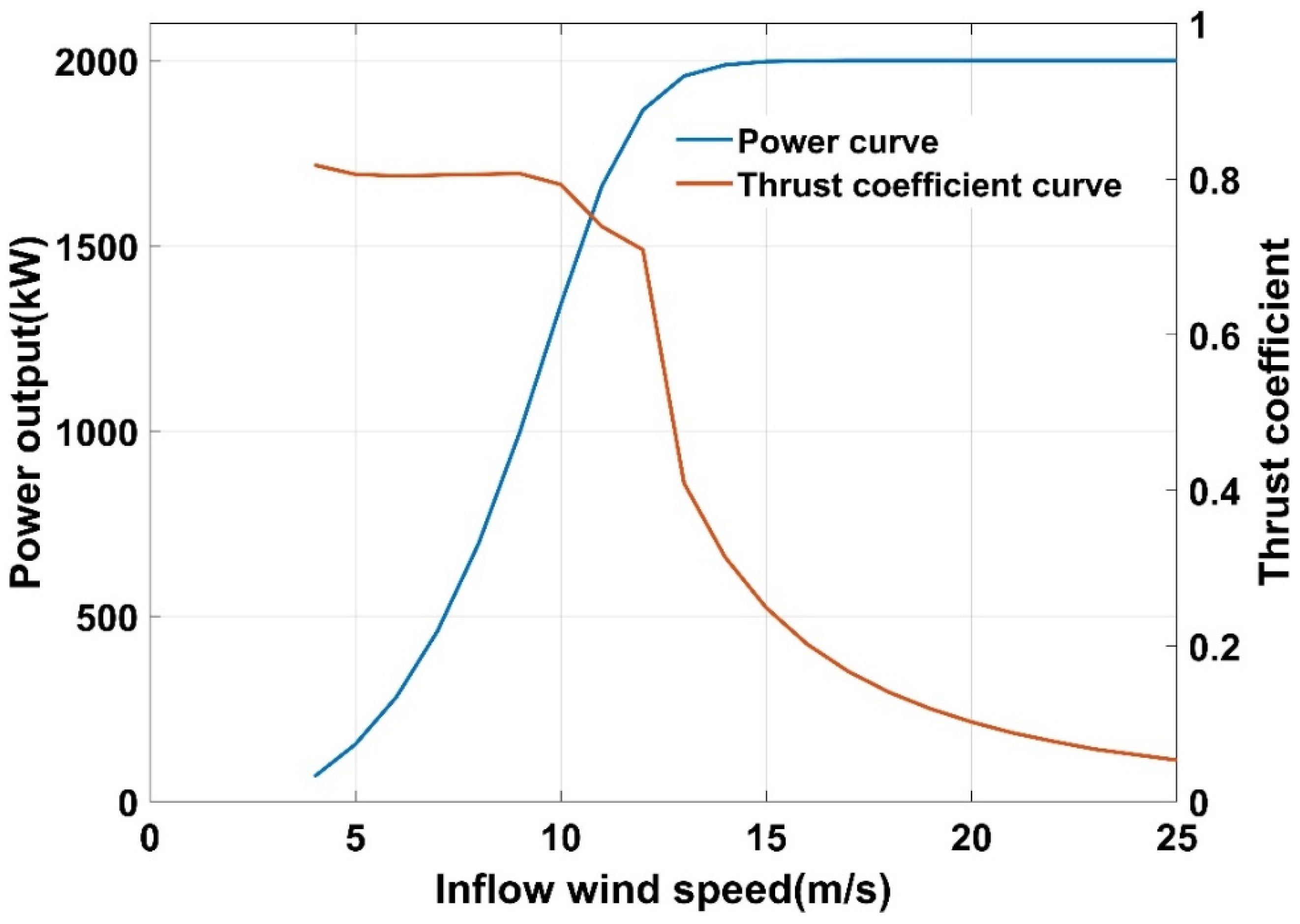
2.2. ADM in PHOENICS

ADM is a reduced-order wind turbine model to replace the actual geometry of a full-scale turbine. It does not need to consider the complicated mesh generation and more grid points, which saves computing resources to a large extent. ADM is derived from the one-dimensional momentum theory. It is assumed that the pressure drops acting on the disc are equivalent to the thrust acting on the rotor. In PHOENICS, the thrust coefficient determines the magnitude of the ADM body force and affects the variation of the flow field. The inflow wind velocity that determines the thrust coefficient is no longer the reference wind speed v_{ref_inflow,i} [22], but is replaced by the wind speed v_disc,i on the disc surface, during wind farm wake simulation. Hence, the ADM in PHOENICS is shown in Equations (9)–(11):

$$v_{ref\_\mathit{inf}low,i}=\frac{v_{disc,i}}{1-a_{x,i}}$$

(9)

$$C_t(v_{disc,i})=4a_{x,i}·\left(1-a_{x,i}\right)$$

(10)

$$S_{disc,i}=-\rho \frac{C_t(v_{disc,i})}{2\mathsf{\Delta }x}{v}_{ref\_\mathit{inf}low,i}^2=-\rho \frac{C_t(v_{disc,i})}{2\mathsf{\Delta }x·{(1-a_{x,i})}^2}{v}_{disc,i}^2$$

(11)

where v_disc,i denotes the AD wind velocity of downwind located rotor i, a_x,i denotes the axial induction factor at the downstream machine i, v_{ref_inflow,i} represents the reference inflow velocity of the machine located in the wake of another wind turbine, and C_t (v_{ref_inflow,i}) is the thrust coefficient based on the reference wind velocity of downstream different located turbine i. S_{disc_,i} is the body force sink acting on the rear rotor i and Δx indicates the thickness of AD, $\mathsf{\Delta }x=0.1D$ [27]—here, D indicates the diameter of AD.

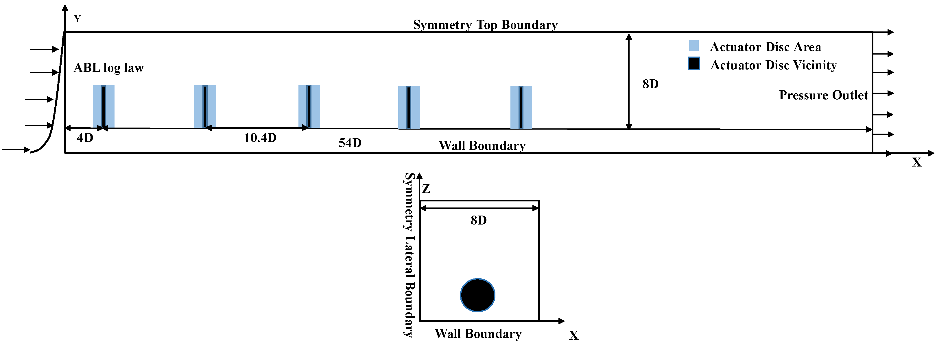
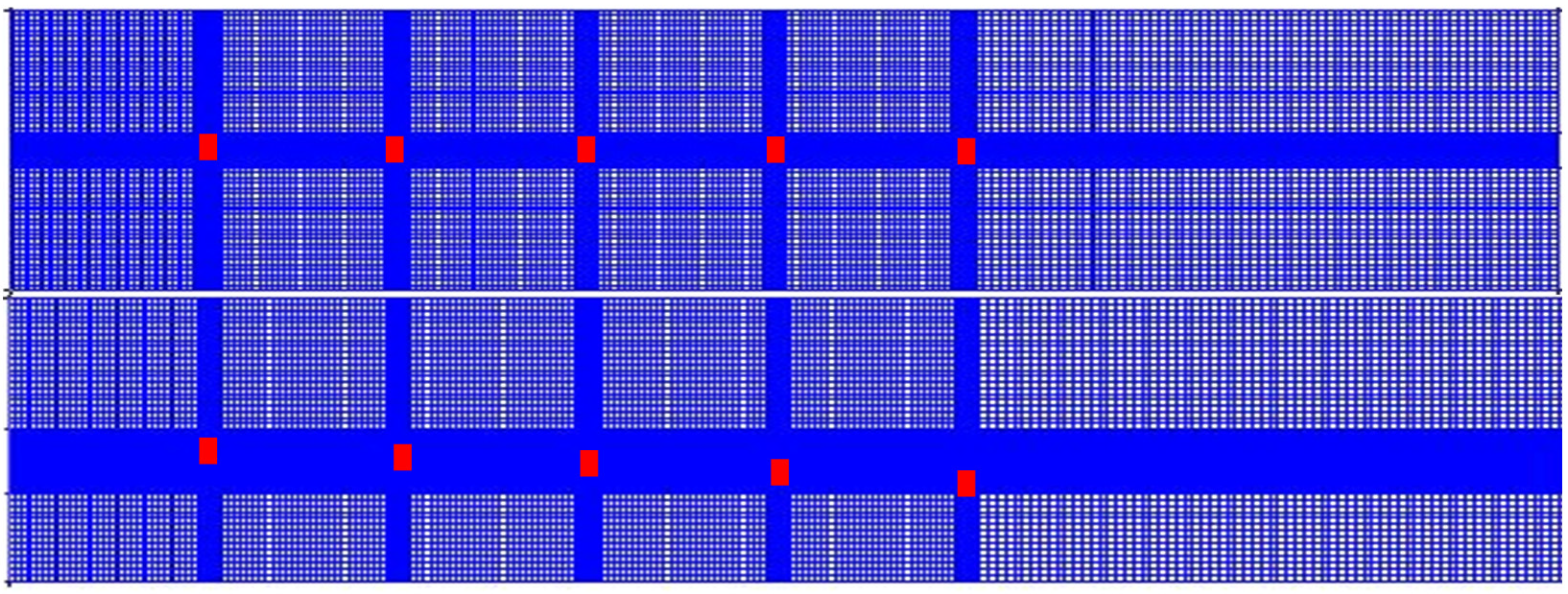
2.3. Computational Domain and Boundary Conditions Settings

With the increase in the number of wind turbines inside wind farms, the computational cost by CFD methods is continuing to grow with the huge grid points in the computational domain. Choosing an appropriate computational domain and boundary conditions is critical for the precision of simulated power production. The measured power output of wind direction (e.g., 312 ± 1°) [28,29] in Horns Rev offshore wind farm selected as a specific case is utilized to describe the computational domain and boundary conditions settings. The computational domain of an aligned case with a wind direction of 312° at Horns Rev offshore wind farm established is a cuboid with a length of 35$D$, a width of 8$D$ and a height of 8$D$, as shown in Figure 1. The spacing from the inlet to the center of upstream first AD is 4$D$. In addition, the distance from the hub center of AD to both lateral symmetry faces is 4$D$ and to the distance of the top boundary is more than 7$D$. The following computational domain and inflow boundary conditions are adopted as the prerequisites for simulations in this case and subsequent cases in this paper, as shown in Figure 1. The logarithmic shear wind profile in the neutral atmospheric turbulent boundary layer [30] can be used as the velocity inlet, as shown in Equation (12).

$$v_0=\frac{v_{*}}{\kappa }\ln \left(\frac{z}{z_0}\right)$$

(12)

where $v_{\ast }$ denotes the freedom inflow friction velocity of the wall surface, and $\kappa$ denotes the von Kármán constant, generally taken as 0.4187 [31]. $z$ is the height in the vertical direction and $z_0$ signifies the aerodynamic roughness length.

2.4. Grid Refinement Study

The coupling model, in which ADM is incorporated into the k-ε model of EI Kasmi, requires local mesh refinement near ADM when carrying out a numerical simulation of wind turbine wakes. According to the previous study on the grid independent of standalone turbine wakes [27], it was demonstrated that the rotor vicinity region of 0.5 $D$ needs 15–30 grid points to be arranged as a prerequisite to guarantee the simulation precision for individual wind turbine wakes. However, grid refinement study remains essential for the numerical simulation of multiple wind turbine wakes to save computational cost, especially for the number of cells in the flow domain. The grid distributions in the crosswind direction and streamwise plane are shown in Figure 2. Five cases are set out in this paper to determine the optimal distribution of grid points in the computational domain for multiple wakes, as shown in

Table 3. Grid refinement study.

Case Setting	Flow Domain Cells/Per Rotor Diameter	Total Number of Grid Points
Case 1	4	1,677,546
Case 2	6	2,414,160
Case 3	10	3,897,894
Case 4	16	5,687,682
Case 5	32	10,540,530

. Additionally, the corresponding power production simulated with the above five different distributed grid points is presented in Figure 3.

It can be found that the normalized power results simulated by the proposed method gradually stabilized with the increase in the number of cells in the flow domain. It is further demonstrated in Figure 3 that the normalized power results are not sensitive to the grid distributions from case 2 to case 5, combined with the local scaling results. Hence, to maximize the saving of computational cost, the settings related to the number of cells for multiple aligned wind turbines inside a wind farm can be referred to as case 2.

3. Test Cases

Five test cases from two offshore wind farms (e.g., Horns Rev offshore wind farm, Nysted offshore wind farm) and one case from Wieringermeer onshore wind farm are used to validate the performance of AD coupling numerical model in this paper. The six test cases used for numerical calculation and the corresponding inflow parameters are shown in

Table 4. Test cases and corresponding input operating parameters.

Case	Description	Measured Data	UH,ꝏ [m/s]	IH,ꝏ [%]	D [m]	z0 [m]	Spacing [m/D]
Offshore wind farm
1	Horns Rev	wd = 270 ± 1°	8	7.7	80	0.0002	7
2	Horns Rev	wd = 222 ± 1°	8	7.7	80	0.0002	9.4
3	Horns Rev	wd = 312 ± 1°	8	7.7	80	0.0002	10.4
4	Nysted	wd = 278°	8	6.3	82.4	0.0002	10.5
5	Nysted	wd = 278°	10	6.3	82.4	0.0002	10.5
Onshore wind farm
6	Wieringermeer	wd = 275 ± 3°	6.59	2.4	80	0.05	3.8

. The details of each case are described below.

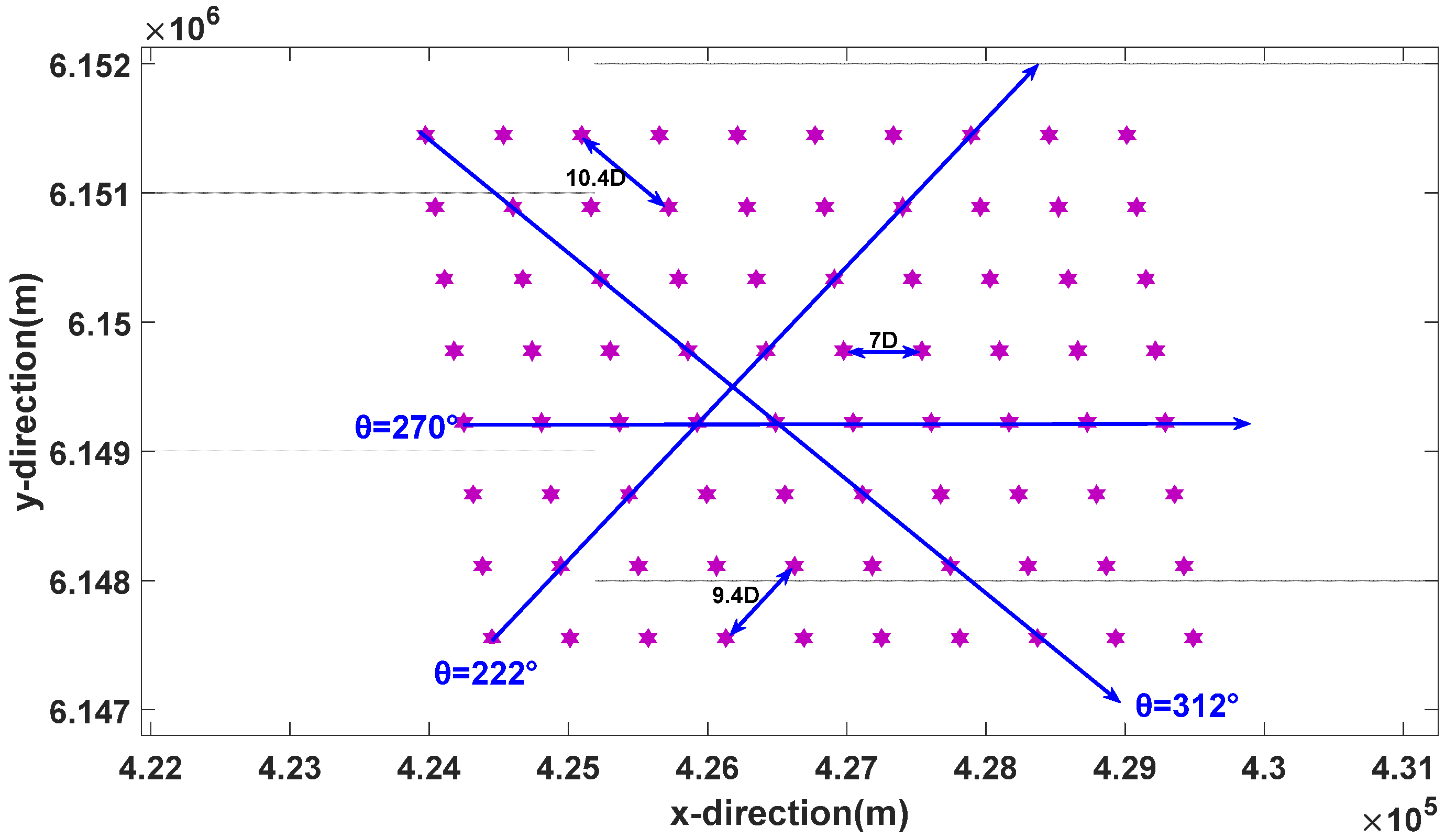
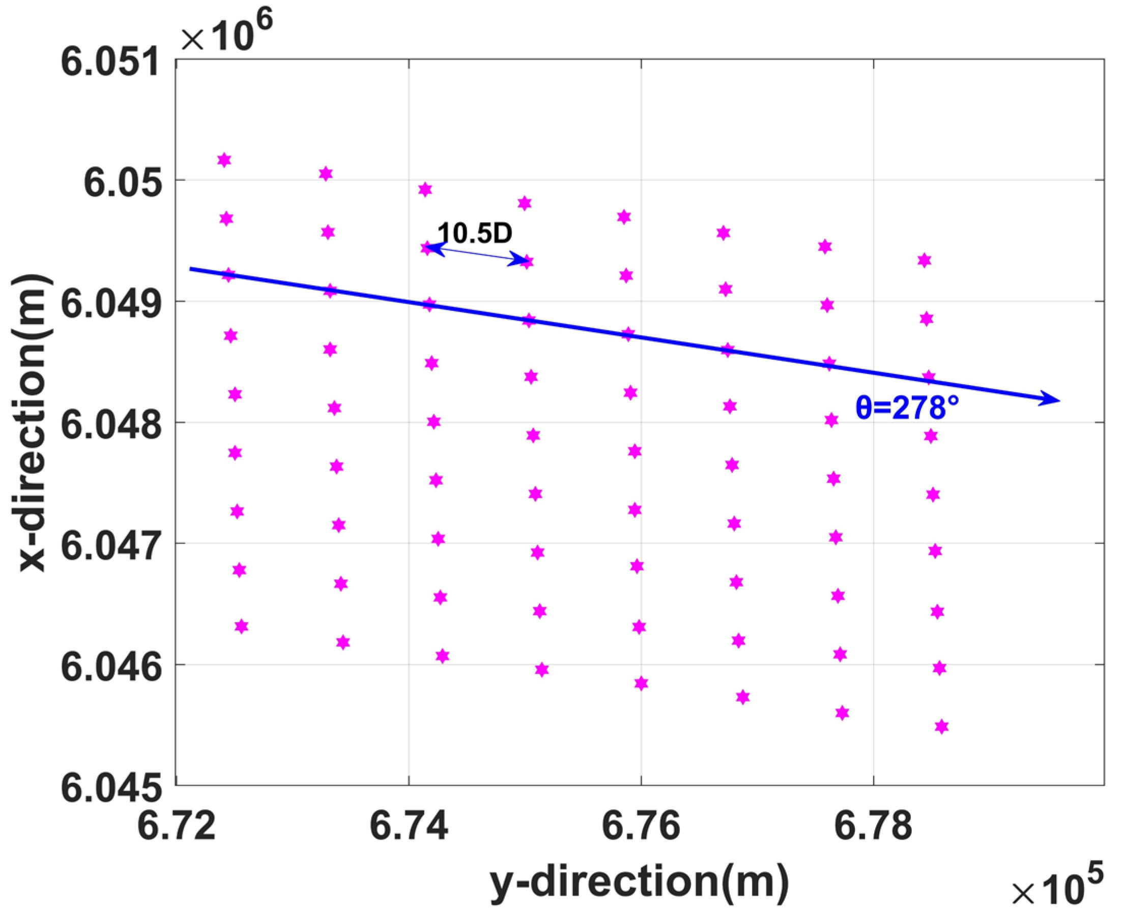
3.1. Horns Rev Offshore Wind Farm Case

The Horns Rev offshore wind farm, located in the Danish waters of the North Sea, is the world’s first large-scale offshore wind farm. It was built in 2002 and occupies an area of 20 square kilometers. The layout of the wind farm is shown in Figure 4. The wind farm has 80 2 MW wind turbines produced by Vestas. The diameter of the Vestas-V80 wind turbine is 80 m, and the hub height is 70 m. The power curve and thrust coefficient curve are shown in Figure 5. Three test cases [28,29] and corresponding input parameters [29,32] are shown in Table 4. It should be noted here that the data collected by the supervisory control and data acquisition (SCADA) system are processed after 10 min of time averaging. Variables such as wind speed and power output are finally sorted according to the data [28] measured by the surrounding meteorological masts.

3.2. Nysted Offshore Wind Farm Case

The Nysted offshore wind farm is a Danish offshore wind farm. It is located in the Baltic Sea, north of the German coastline and 10 km from the coastline of the island of Lolland in southeastern Denmark. It was built in 2003 and has a total installed capacity of 165.6 MW, consisting of 72 Bonus 2.3 MW wind turbines manufactured by Siemens Wind Power. The 72 wind turbines are arranged in a parallelogram grid with nine rows and eight columns, as shown in Figure 6. Each turbine is a Bonus 2.3 MW wind turbine, with the diameter of 82.4 m and a height of 68.8 m. The data of power and thrust coefficient are from reference [33], thus the power curve and thrust coefficient curve of the Bonus 2.3 MW wind turbine can be shown in Figure 7.

In this paper, two flow test cases with an inlet wind direction of 278° and two wind speeds (e.g., 8 m/s and 10 m/s) at the Nysted offshore wind farm [34] are available to carry out the wind farm wake simulation based on the proposed AD coupling numerical model. The two cases based on the two undisturbed inflow wind velocities and corresponding settings of input parameters are represented in Table 4.

To realize the numerical simulation of the wake flow field for the corresponding cases, the computational domain of the Nysted offshore wind farm with an inlet wind direction of 278° is carried out here in combination with the grid refinement study in Section 2.4. Grids of the computational domain is shown in Figure 8. The entire computational domain adopts hexahedral grid elements, and the total number of cells is about 5.4 million. Additionally, the number of cells in the streamwise direction is 708, 80 grid points are distributed along the vertical direction and spanwise direction, respectively.

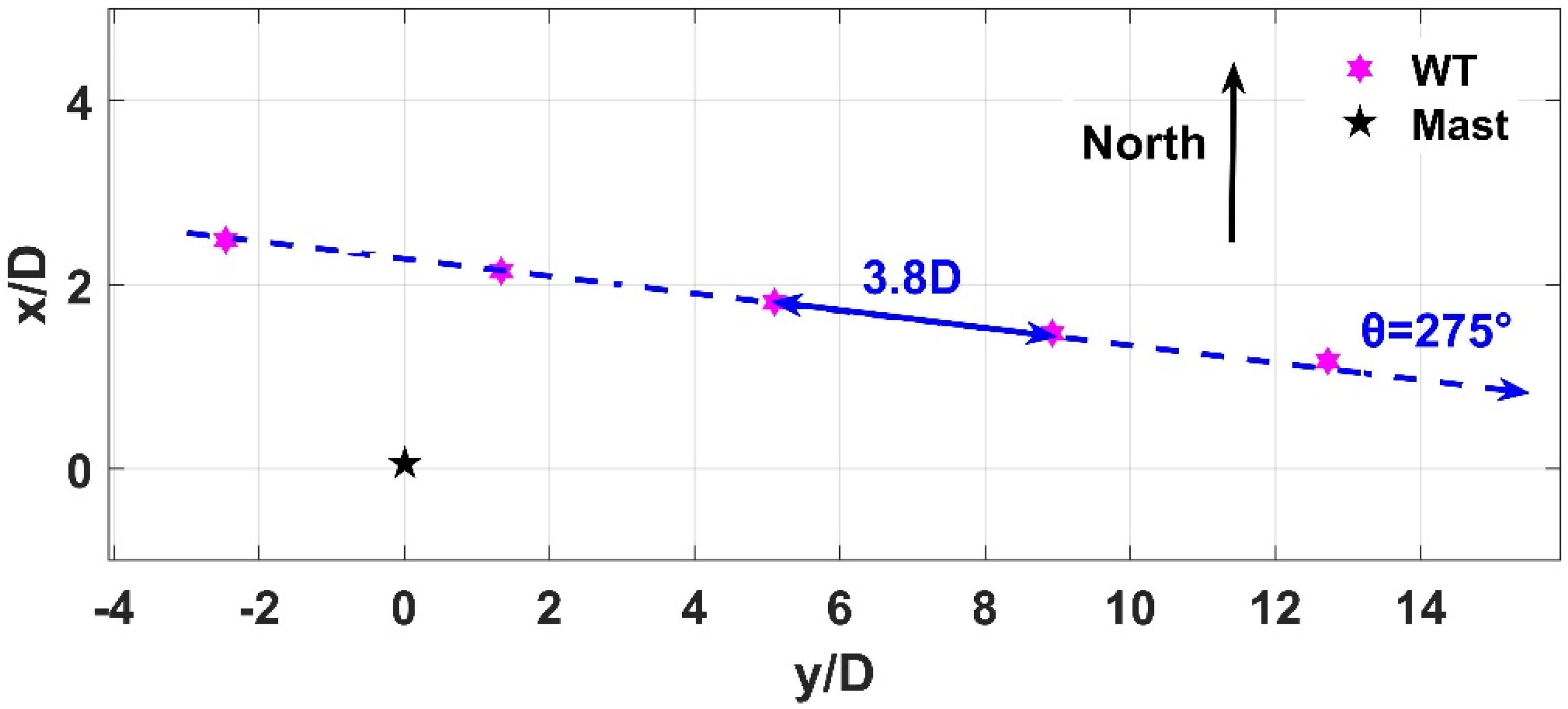
3.3. Wieringermeer Onshore Wind Farm Case

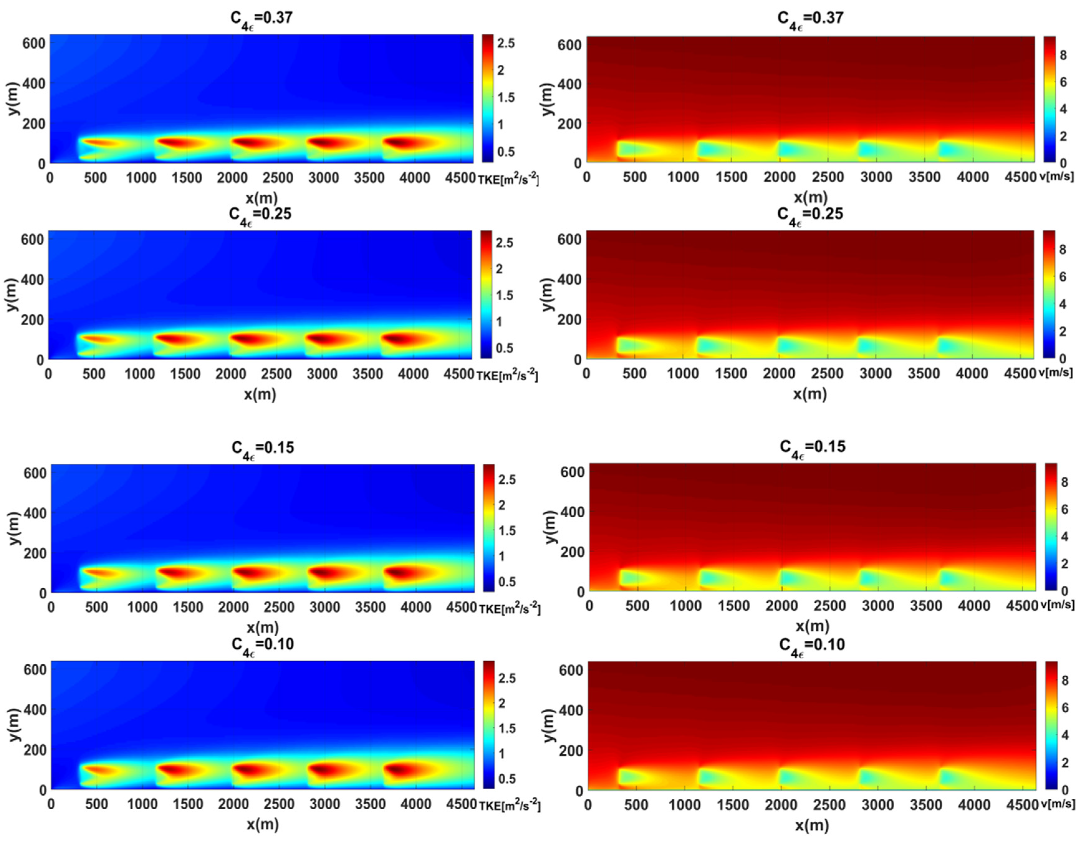
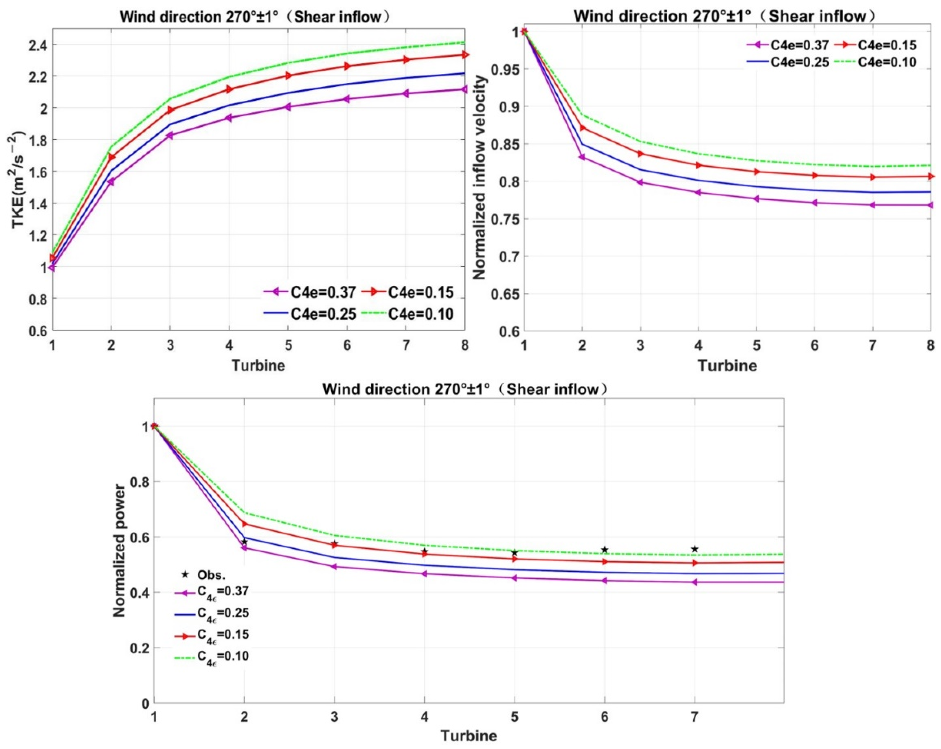
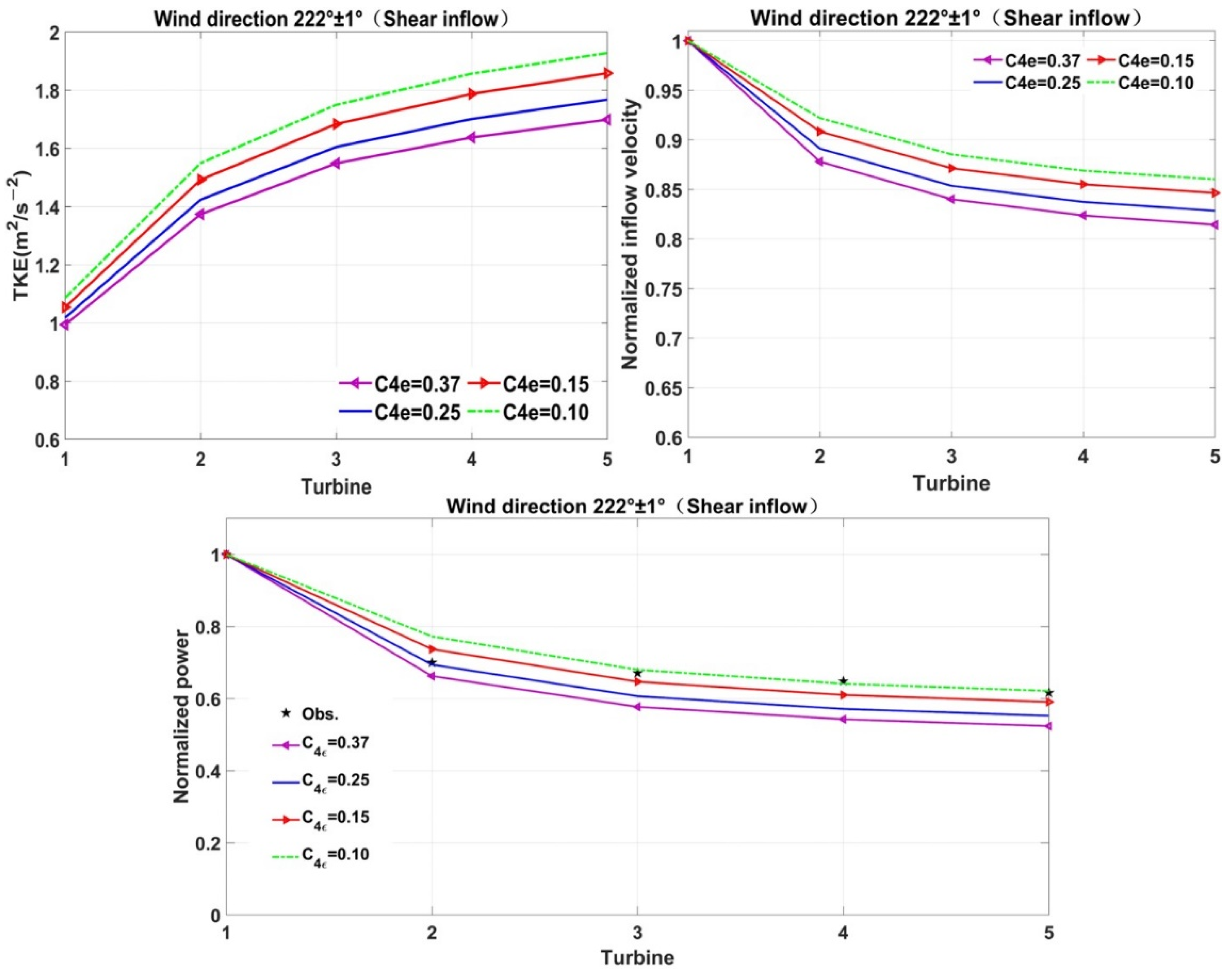
An experimental wind farm consisting of five Nordex 2.5 MW wind turbines is located in Wieringermeer. The wind farm is operated and maintained by the Energy Research Centre of the Netherlands (ECN). The wind farm is located on relatively flat farmland in the northwest of the Netherlands. The specific layout is shown in Figure 9. The diameter of the rotor and the hub height of the Nordex 2.5 MW wind turbine are both 80 m. The data of power output and thrust coefficient are from references [14,35], and thus the power curve and thrust coefficient curve can be presented in Figure 10. In this wind farm, the spacing between adjacent turbines in the prevailing wind direction, 275°, is 3.8 D. In addition, a met mast in Figure 9 can be utilized to measure undisturbed inflow wind conditions. Almost five years of measurements on the wind farm and the measurement power data after ten-minute averaging can be used for numerical model validation, according to the published results from Schepers et al. [36]. A power output case with a wind direction of 275 ± 3° is selected to simulate the wind farm wake using the proposed AD coupling numerical model in this paper.

Different from the layout types of the previous two wind farms, the ECN test wind farm is an onshore wind farm with a tight spacing arrangement. The downstream-located wind turbines are fully or partially covered by the wake of the upstream machines when the angle of the wind direction is measured within a deviation angle of ±3°. Hence, grids distribution of the computational domain with the inflow wind direction of 275 ± 3° (presented in Figure 11) can be divided into two grid distributions with a wind direction of 275° and 278°, based on the grid independence study in Section 2.4. Since the computational domain grid with the inflow wind direction of 272° is symmetrical to that with the wind direction of 278°, it is no longer shown here. The upper part is the grid of the computational domain with a wind direction of 275°, and the total number of cells is 2,150,148. The number of cells in the streamwise direction is 369; 80 nodes are distributed vertically, and the number of nodes in the spanwise direction is also 80. The lower part is the grid distribution of the computational domain with a wind direction of 278°. Its total number of cells is 2,443,584. The number of grid nodes in the flow direction is 363, the number of nodes in the vertical distribution is 80, and the number of cells in the spanwise direction is 92.

3.4. Effects of Parameter C_4ε on Wind Farm Wake Simulation Considering Six Test Cases

As mentioned above, few scholars have further studied how the parameter C_4ε in the k-ε turbulence model of Kasmi affects the turbulent kinetic energy (TKE) in the wake superposition areas, and the influence of TKE on the recovery of the wake velocity of wind farms. A reasonable calibration of the parameter C_4ε in the improved k-ε turbulence model is crucial to accurately simulate the power deficits caused by the effects of multiple wakes.

Hence, two offshore scenarios cases including Horns Rev and Nysted and an onshore wind farm case from Wieringermeer were adopted in Section 3, aiming to quantitatively investigate the effects of the parameter C_4ε on the power out loss of wind farms. The six test cases based on different parameters C_4ε and the corresponding inflow parameters are shown in

Table 5. Six case settings considering different parameter C_4ε values.

Case	Description	C4ε	UH,ꝏ [m/s]	IH,ꝏ [%]	D [m]	z0 [m]	Spacing [m/D]
1	Horns Rev (wd = 270 ± 1°)	0.37, 0.25, 0.15, 0.10	8	7.7	80	0.0002	7
2	Horns Rev (wd = 222 ± 1°)	0.37, 0.25, 0.15, 0.10	8	7.7	80	0.0002	9.4
3	Horns Rev (wd = 312 ± 1°)	0.37, 0.25, 0.15, 0.10	8	7.7	80	0.0002	10.4
4	Nysted (wd = 278°)	0.37, 0.25, 0.15, 0.10	8	6.3	82.4	0.0002	10.5
5	Nysted (wd = 278°)	0.37, 0.25, 0.15, 0.10	10	6.3	82.4	0.0002	10.5
6	Wieringermeer(wd = 275 ± 3°)	0.37, 0.25, 0.15, 0.10	6.59	2.4	80	0.05	3.8

. The wind farm power measurement values mentioned above are compared with the results of the proposed AD coupling numerical model, and the parameter C_4ε is calibrated. In addition, the mean absolute percentage error (MAPE) and root mean square error (RMSE) are used to quantify the prediction accuracy of power production and the deviation between the simulation results and the measured values, respectively.

$$e_{Power\_MAPE}=\frac{1}{M}{\displaystyle \sum _{i=1}^M\left|\frac{P_w(i)-\overline{P_w}(i)}{\overline{P_w}(i)}\right|}\times 100\%$$

(13)

$$e_{Power\_RMSE}=\sqrt{\frac{1}{M}{\displaystyle \sum _{i=1}^M{\left(P_w(i)-\overline{P_w}(i)\right)}^2}}\times 100\%$$

(14)

where $P_w(i)$ denotes the normalized power simulation values of downstream different located turbines and ${\overline{P}}_w(i)$ denotes observed power values.

Table 6. Error analysis of power simulation of six cases with different parameter C_4ε values.

	${\mathit{C}}_{4\mathit{\epsilon }}=0.37$	${\mathit{C}}_{4\mathit{\epsilon }}=0.25$	${\mathit{C}}_{4\mathit{\epsilon }}=0.15$	${\mathit{C}}_{4\mathit{\epsilon }}=0.10$
Case 1
$(e_{Power\_MAPE}/[\%])$	14.35	10.04	5.74	5.16
$(e_{Power\_RMSE}/[\%])$	9.16	6.54	3.58	4.25
Case 2
$(e_{Power\_MAPE}/[\%])$	10.11	6.51	3.77	2.73
$(e_{Power\_RMSE}/[\%])$	7.72	5.31	2.85	3.29
Case 3
$(e_{Power\_MAPE}/[\%])$	8.81	5.45	1.99	2.86
$(e_{Power\_RMSE}/[\%])$	7.88	5.40	2.73	3.43
Case 4
$(e_{Power\_MAPE}/[\%])$	8.69	5.77	4.59	8.11
$(e_{Power\_RMSE}/[\%])$	5.47	4.13	4.52	6.44
Case 5
$(e_{Power\_MAPE}/[\%])$	7.37	5.77	4.06	8.53
$(e_{Power\_RMSE}/[\%])$	4.86	3.41	4.18	6.36
Case 6
$(e_{Power\_MAPE}/[\%])$	15.37	12.70	10.27	16.89
$(e_{Power\_RMSE}/[\%])$	5.83	3.91	3.51	5.34
Average Error
$(e_{Power\_MAPE}/[\%])$	10.78	7.71	5.07	7.38
$(e_{Power\_RMSE}/[\%])$	6.82	4.78	3.56	4.85

shows the error effects of different parameter C_4ε values on the power output of wind turbines under six cases. It can be found that the average $e_{Power\_MAPE}$ of the proposed actuating disc coupling numerical model is only 5.07%, and the corresponding average $e_{Power\_RMSE}$ drops to 3.56% compared with the measured power output, when C_4ε is 0.15. As the parameter C_4ε reduces, the mean $e_{Power\_MAPE}$ and mean $e_{Power\_RMSE}$ show a decreasing and then upward tendency. In the first three cases of the Horns Rev offshore wind farm, the model corresponding to the reduced parameter C_4ε significantly improves the accuracy of the turbines’ power output simulation as the distance between adjacent rotors increases. Combining with the three wind direction cases, it can be seen that the average power prediction error $e_{Power\_MAPE}$ with the given wind directions is only 3.83%, and the mean $e_{Power\_RMSE}$ is only 2.73%, when C_4ε = 0.15. Similar to the Horns Rev offshore wind farm, the Nysted offshore wind farm also adopts a widely spaced wind farm layout, but the difference is that the Nysted wind farm uses a Bonus 2.3 MW wind turbine with a larger installed capacity. In cases 4 and 5, the simulation accuracy of power output corresponding to the parameter C_4ε is gradually improved with the increase in the inflow wind speed. As the parameter C_4ε changes from 0.37 to 0.15, the simulated results of the power output gradually approach the measured values. The simulated power outputs compare well with the measured results when C_4ε = 0.15, with an average $e_{Power\_MAPE}$ of only 4.33% and an average $e_{Power\_RMSE}$ of 4.35%. Differing from the above two cases of offshore wind farms, case 6 is an onshore wind farm case. The lower inflow turbulence intensity and the narrow spacing of rotors within the farm bring about serious power loss in the downwind machines. Nevertheless, the model built in this paper can still effectively simulate the measured power output of different turbines in a given wind direction. When the parameter C_4ε is 0.15, the numerical simulation result is the closest to the measured power value, the $e_{Power\_MAPE}$ is 10.27%, and the $e_{Power\_RMSE}$ is only 3.51%.

4. Results and Discussion

The results of six cases from two offshore wind farms and one onshore wind farm are discussed separately in the following sections. In addition, the influence of parameter C_4ε on the power output of wind turbines in all cases is discussed further.

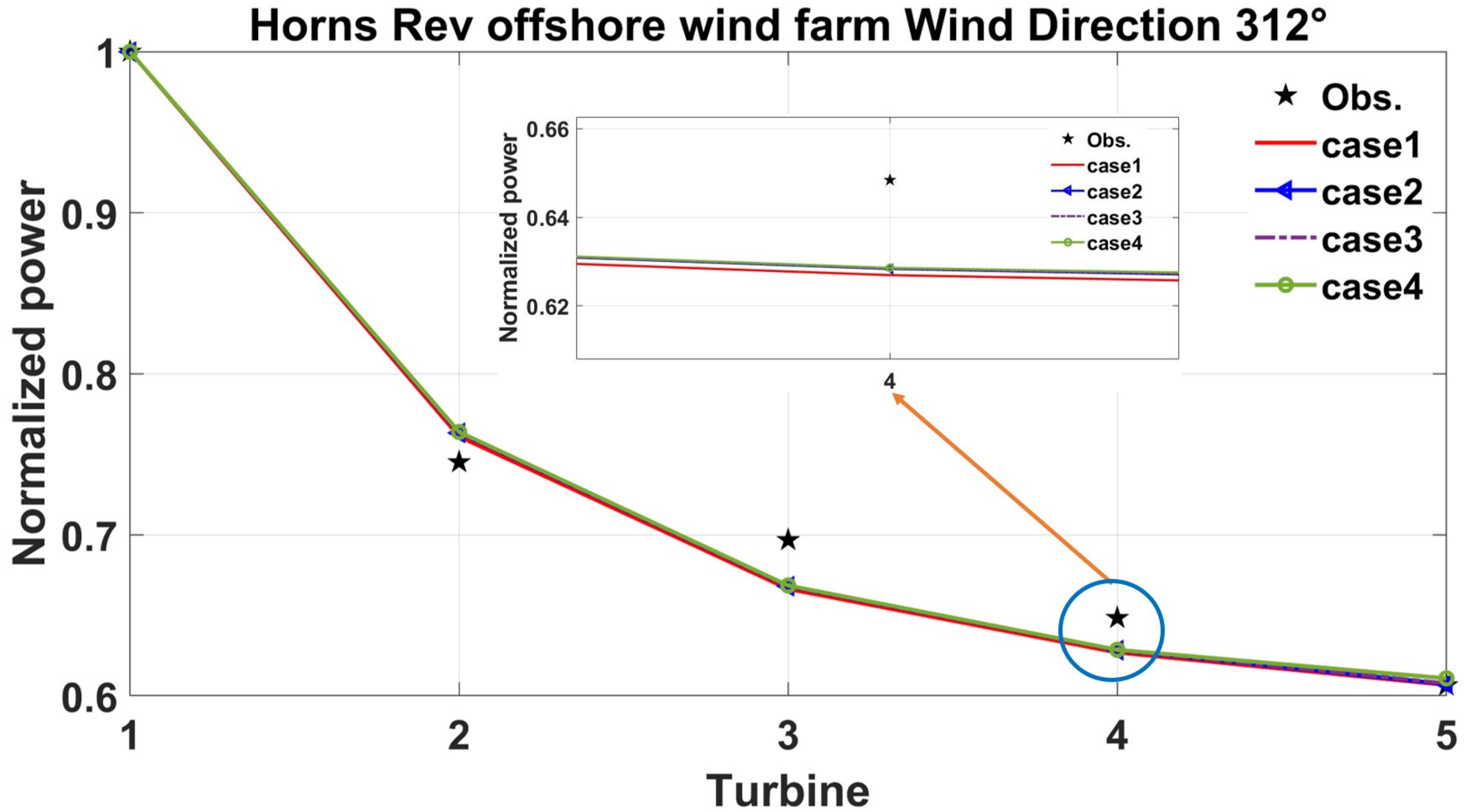
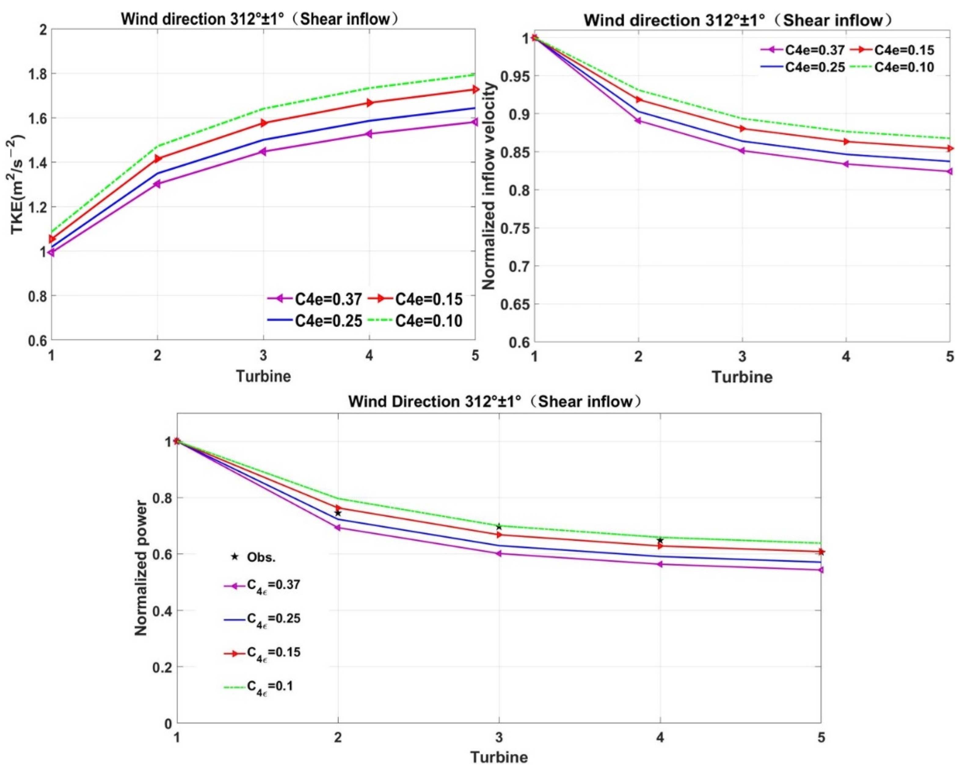
4.1. Horns Rev Offshore Wind Farm

Initially, we discuss the influence of parameters C_4ε on the turbulent kinetic energy and the wake velocity of the flow field under different wind directions from the perspective of numerical simulation contours. Subsequently, the inflow wind speed and power output of downstream-located rotors are calculated with the AD and curves of power and thrust coefficient. Finally, the power output simulation results of different parameters C_4ε are compared with the measured power values.

Contours of TKE and streamwise velocity in the vertical direction for different C_4ε values under shear inflow conditions when the wind direction is 270° are shown in Figure 12. As can be seen from Figure 12, the shear effect accelerates the wake turbulent dissipation of the first rotor, and the TKE on the lower parts of AD is lower than that generated on the upper part of AD. In addition, the TKE presents an obvious asymmetrical distribution at the near wake region of the first AD. The main reason for this is that the logarithmic shear inflow has a high-velocity gradient on the upper parts of the wind rotor. Furthermore, the generation of wake TKE on the upper parts of the rotor is further increased due to the blockage effects. The logarithmic shear induces a small velocity gradient on the lower parts of the turbine, where it makes a limited contribution to the wake TKE. As the turbulence develops downstream, the TKE from the environment and the wake region accelerates the mixing intensity, thereby causing the wake velocity deficits to gradually decrease with the downstream distance. Affected by the upstream rotor wake, the velocity loss in the wake region of the second turbine further increases. Additionally, the TKE shows an upward trend. The flow interaction between the adjacent turbines further increases the TKE in the near-wake region of the downwind machines located in the superposition area of two or more upstream rotors. The wake deficits further aggravate, resulting in a further decrease in the inflow wind speed from the downstream rotors. The additional source term (Equation (8)) in this paper is active in the vicinity of wind turbines. It can control the relationship between turbulence generation and dissipation when the multiple wind turbine wakes interact, thereby affecting the wake recovery degree of each downstream-located turbine. With the decrease in the parameter C_4ε in the source term, the impact range of TKE in the wake region of each rotor under a given wind direction gradually decreases. In addition, the extreme point of TKE is close to the rotor, and the wake recovery rate of the corresponding turbine is accelerated. This indicates that the reduction in parameter C_4ε in the dissipative source term contributes significantly to the generation of TKE caused by the interaction of multiple rotors.

Figure 13 presents the comparison of TKE and wake distribution in the vertical plane with different C_4ε under shear inflow conditions when the wind direction is 222°. As the spacing between adjacent rotors increases from 7 D to 9.4 D, the influence area of TKE in the wake region of each turbine gradually decreases, and atmospheric turbulence plays a dominant role in wake recovery. In addition to the first rotor, the TKE in the wake region of each downstream turbine still maintains a non-uniform distribution on the upper and lower part of the rotor. Furthermore, the TKE in the wake area upon the upper part of the rotor is relatively large. The main reason for this is that the larger the velocity gradient that appears over the upper part of the rotor, the more obvious the velocity loss is. The existence of the additional dissipative source term dominates the amount of TKE generated near each rotor for a given wind direction. With the decrease in the parameter C_4ε, the generation range of TKE in the vicinity of the control rotor becomes smaller, but the TKE near the rotor becomes larger, and the wake recovery rate of the downstream-located machines is less affected by the near-wake. In addition, the increased interwind turbine spacing can promote the wake recovery of each downstream rotor effectively.

Contours of TKE and wake distribution on the vertical plane with different parameters C_4ε under shear inflow conditions when the wind direction is 312° are presented in Figure 14. With the further increase in the spacing between adjacent turbines from 9.4 D to 10.4 D, the effects of atmospheric turbulence on wake recovery are further enhanced. Similar to Figure 13, the extreme point of TKE in the wake region of each downstream-located rotor goes up and the scope of influence gradually approaches the wind rotor, with the reduction in parameter C_4ε. The increased interwind turbine spacing can effectively slow down the generation of TKE from the wake of each downstream rotor and promote wake recovery.

To sum up, the values of the different parameters C_4ε for the above three inflow wind directions have obvious control effects on the generation of wake TKE and the recovery of wake velocity. The decrease in the parameter C_4ε is beneficial to the forward shift of the extreme value point and influences the range of TKE in the wake region of the wind rotor and gradually approaching the wind rotor. Additionally, the atmospheric turbulence gradually mixes into the wake region, which decelerates the generation rate of TKE in the wake region and accelerates the recovery degree of wind turbine wake, with the increase in the downstream distance.

Figure 15, Figure 16 and Figure 17 quantitatively present the effects of different parameter C_4ε values on TKE, inflow wind speed and power output under three wind directions (e.g., 270 ± 1°, 222 ± 1°, and 312 ± 1°), respectively. As can be seen from Figure 17, as the TKE at the hub height of each downwind-located turbine gradually increases, the inflow wind speed and power output tend to reduce and finally stabilize due to the turbulence interaction from adjacent turbines, when the wind direction is 270 ± 1°. With the decrease in the parameter C_4ε, the TKE at the hub height of other downstream rotors gradually descends, and the inflow wind speed and power output gradually go up. As mentioned above, the decrease in the parameter C_4ε can efficiently promote the increase in TKE in the vicinity of each downwind rotor and facilitate the rise in inflow wind speed and power generation. The final stabilization of the power output is attributed to the dominant role of ambient turbulence in the atmosphere, and the mixing of wake turbulence with ambient turbulence is no longer intense.

It can be concluded from the power simulation results that the second rotor is affected by the wake effect of the upstream machine, resulting in a serious deficit of power generation in Figure 15. The parameters C_4ε = 0.37 and C_4ε = 0.25 in the built model correspond to the power output calculated by the proposed AD coupling numerical model which is the closest to the measured power of the second turbine. However, the power output generated by the other rotors in the streamwise direction tends to be stable, due to the combined effect of wake superposition and atmospheric turbulence. The power output simulation results under the above two parameters (e.g., C_4ε = 0.37, C_4ε = 0.25) have a large deviation from the measured power. From the overall simulation effect of power output, the calculated power output based on the parameter C_4ε = 0.15 is in the best agreement with the measured power, except for the second rotor. However, it is undeniable that the power output simulation results of the second unit have a large deviation from the measured values when C_4ε is 0.15, and the $e_{Power\_MAPE}$ reaches 11.13%. The main reason for this is that the dissipation source term corresponding to the smaller parameter C_4ε leads to the accelerated dissipation of turbulent kinetic energy in the wake region, which in turn promotes the accelerated wake recovery. Due to the limited spacing between the second turbine located in the wake region and the upstream one, it is difficult for the first rotor to obtain enough energy from the atmospheric environment to promote its wake recovery, resulting in lower inflow wind velocity and reduced power generation at the second turbine. Eventually, the power simulation results corresponding to the smaller parameter C_4ε have a large deviation from the measured power.

As the interwind turbine spacing increases from 7 D to 9.4 D, the simulated values of TKE at hub height of each downwind rotor gradually decrease, the influence area of ambient turbulence increases, and the level of wake recovery is further improved. In addition, the power simulation results also increase. Combined with Table 6 and Figure 16, it can be found that as the distribution of parameter C_4ε decreases from 0.37 to 0.10, the $e_{Power\_MAPE}$ decreases gradually and the $e_{Power\_RMSE}$ reduces first and then ascends. The comprehensive analysis demonstrates that when C_4ε = 0.15, the power simulation results compare well with the actual measurement results, with prediction error $e_{Power\_MAPE}$ of only 3.77% and $e_{Power\_RMSE}$ of 2.85%. Of course, similar to the case with wind direction of 270 ± 1°, the simulated power corresponding to a C_4ε of 0.15 overpredicts the measured power of the second rotor, but the prediction error gradually decreases. It shows that the increased spacing causes the ambient turbulence play a role in promoting wake recovery.

The further increased spacing between adjacent turbines drives the ambient turbulence-dominated range to be further expanded and the vicinity range affected by parameter C_4ε is further compressed when the wind direction is 312 ± 1° and the spacing is 10.4 D. In addition, the value of TKE at hub height from each downstream machine is further reduced. In terms of power output verification, it can also be found that the power simulation results have the smallest deviation from the measured values when C_4ε = 0.15, the $e_{Power\_MAPE}$ is less than 2% and $e_{Power\_RMSE}$ is only 1.76%. The simulation results of the power output of the second machine corresponding to C_4ε of 0.15 gradually match with the measured power data as the spacing between the adjacent turbines increases in Figure 17. This indicates that the reduction in the parameter C_4ε can effectively control the mixing intensity of wake turbulence and ambient turbulence, and the accurate prediction effect of the power output from the rear row rotors is obvious.

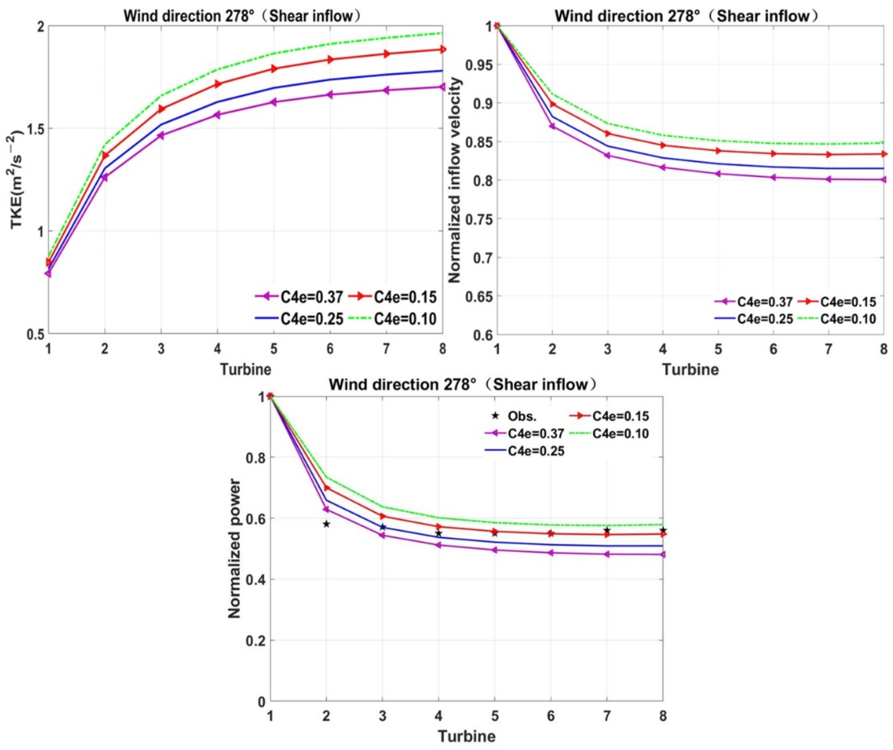
4.2. Nysted Offshore Wind Farm

Figure 18 reveals the effect of parameter C_4ε on TKE, inflow wind speed, and power output when the inflow wind direction is 278° and the undisturbed inflow wind speed is 8 m/s. The Nysted offshore wind farm is similar to the Horns Rev offshore wind farm in that it is a widely spaced, large-scale offshore wind farm. However, Nysted Offshore Wind Farm employs the Bonus 2.3 MW wind turbine with a larger installed capacity under similar input conditions to those of the Horns Rev Offshore Wind Farm. This results in a larger TKE and power deficits, and lower inflow wind speed at the hub height of the streamwise located rotors. However, the TKE, inflow velocity, and power output all increase at the hub height of the downstream-located machines, with the decrease in the parameter C_4ε. As the incoming wind speed increases from 8 m/s to 10 m/s, the TKE, inflow wind speed, and power generation at the hub height of the downwind turbines further increase, as presented in Figure 19.

In terms of the quantitative evaluation of power output, it can be seen in Table 6 and Figure 18 that when the parameter C_4ε is 0.15 in case 4, the simulation result of the generated power output is the closest to the measured power value, the $e_{Power\_MAPE}$ is 4.59%, and the $e_{Power\_RMSE}$ reaches 4.52%. Different from the Horns Rev offshore wind farm case, the power deficit of the second rotor affected by the wake increases significantly due to the lower ambient turbulence in the Nysted offshore wind farm test case. The power simulation results corresponding to the parameter C_4ε = 0.15 overestimate the actual power output results, and the $e_{Power\_MAPE}$ is as high as approximately 20%. However, the power simulation results calculated by other turbines in the downwind direction are in good agreement with the measured power values, and the $e_{Power\_MAPE}$ does not exceed 3%. As the inflow wind speed increases from 8 m/s to 10 m/s, the power simulation error of the power output from the second machine further decreases. In particular, when the parameter C_4ε is 0.15, the power prediction error $e_{Power\_MAPE}$ drops to about 17%. Combining cases 4 and 5, the reduction in the ambient turbulence intensity is likely to slow down the speed recovery of the far wake, resulting in an increase in the power loss of the downstream turbines. However, with the increase in the inflow wind speed, the environmental average velocity accelerates the recovery of the wake, and the power loss of the downstream rotors is further reduced, and the simulated result of the power output gradually approaches the measured value.

4.3. Wieringermeer Onshore Wind Farm

The effects of the parameter C_4ε on TKE, inflow wind speed and power output when the inflow wind direction of is 275 ± 3° at the ECN onshore wind farm are presented in Figure 20. The ECN onshore wind farm has a flat terrain and low inflow turbulence intensity, which makes it difficult to promote the upstream wind turbines to generate higher power output. The relatively narrow spacing between adjacent turbines results in a strong wake superposition effect on the downstream turbines. The power loss is even more serious.

In terms of power output evaluation, differing from the previous offshore wind power output cases, the actual power output of the second turbine is more serious due to the lower ambient inflow turbulence intensity and narrow spacing between adjacent turbines on the Wieringermeer onshore wind farm. The simulated power results corresponding to different parameter C_4ε values are compared with the measured power, and it is found that as the parameter C_4ε decreases, the corresponding simulated power shows an increasing trend. However, the simulated power value corresponding to a C_4ε of 0.15 significantly overestimates the measured power results of the second machine, and the prediction error $e_{Power\_MAPE}$ is as high as 41.27%. This shows that the decrease in the parameter C_4ε is not conducive to the accurate evaluation of the power output from the turbine that is in the wake region. Nevertheless, except for the second unit, the power output prediction error $e_{Power\_MAPE}$ corresponding to C_4ε = 0.15 is only 3.36%. In general, when C_4ε is 0.15, the model built in this paper can still precisely simulate the measured power of different units in given wind directions.

5. Conclusions

The k-ε turbulence model of EI Kasmi coupling with ADM within the RANS framework can be applied in layout optimization, micro-sitting, and power generation assessment during the design stage of modern wind farms. However, few researchers have further studied how the parameter C_4ε in the k-ε model of EI Kasmi affects TKE in the superposition areas and the recovery of wind farm wake velocity. To this end, this paper adopts advanced ADM in PHOENICS combined with the k-ε model of EI Kasmi to investigate the influence of parameter C_4ε on the wake simulation of wind farms under different scenarios (e.g., two offshore wind farms, one onshore wind farm). The following main conclusions are drawn:

(1)

The decreased parameter C_4ε makes the generation scope of TKE in the vicinity of the turbine smaller, but the TKE near the rotor becomes larger, and the wake recovery rate of the downstream turbine is less affected by the near wake. As the interwind turbine spacing increases, the influence area of TKE in the wake region of each downstream machine gradually reduces, and atmospheric turbulence plays a dominant role in wake recovery.

(2)

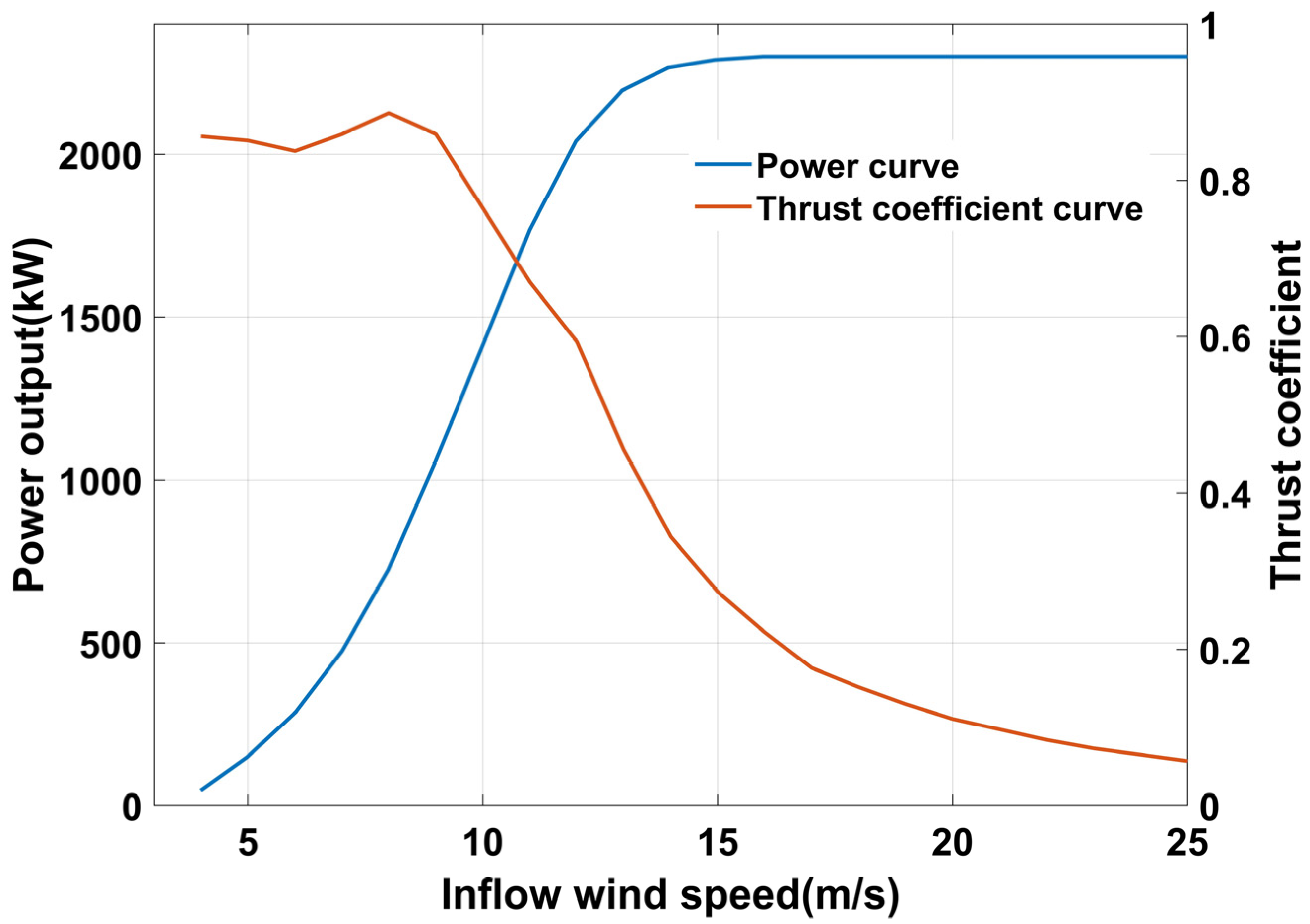
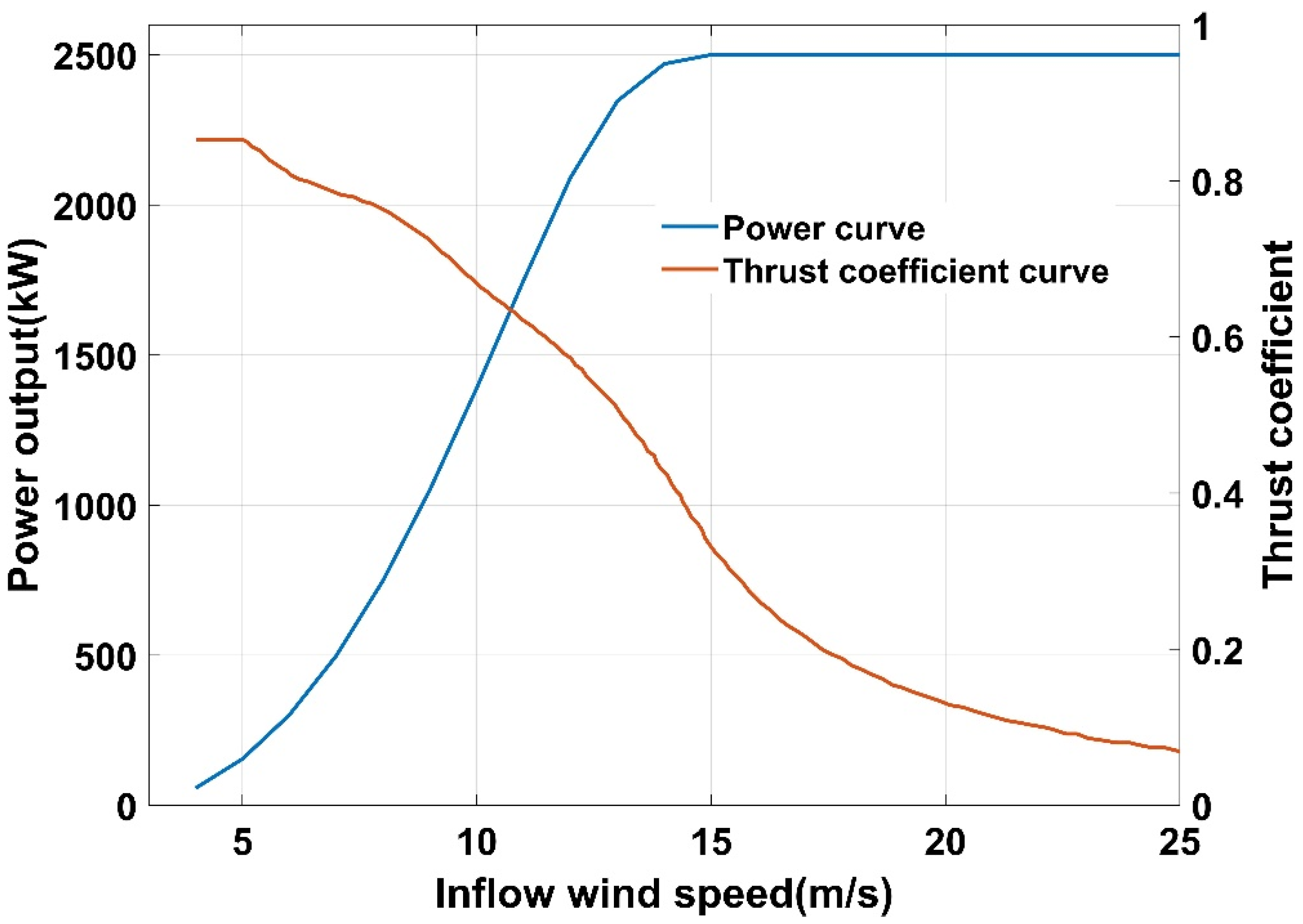
The decrease in parameter C_4ε can efficiently promote the increase in TKE in the vicinity of each downwind rotor and facilitate the rise of inflow wind speed and power generation. The final stabilization of the power output is attributed to the dominant role of ambient turbulence in the atmosphere, and the mixing of wake turbulence with ambient turbulence is no longer intense. In addition, the increase in the ambient undisturbed inflow wind velocity can promote the further improvement of TKE, inflow wind speed, and power generation at the hub height of downstream-located rotors. Furthermore, an increase in TKE at the hub height of downwind rotors thereby causes inflow wind speed reduction, and the power deficits increase when the ambient undisturbed inflow wind speed passes through a larger-scale wind turbine.

(3)

The coupling numerical model in this paper is validated by six sets of measured power data from three wind farms. It has been found that when the parameter C_4ε equals 0.15, the simulated power results are compared well with the measured power outputs. The proposed coupling numerical model and the further calibration of the parameter C_4ε can provide essential technical support for micro-siting, operation control, and power output prediction on wind farms.

References

1. Archer, C.L.; Vasel-Be-Hagh, A.; Yan, C.; Wu, S.; Pan, Y.; Brodie, J.F.; Maguire, A.E. Review and evaluation of wake loss models for wind energy applications. Appl. Energy 2018, 226, 1187–1207. [Google Scholar] [CrossRef]
2. Tian, J.; Zhou, D.; Su, C.; Soltani, M.; Chen, Z.; Blaabjerg, F. Wind turbine power curve design for optimal power generation in wind farms considering wake effect. Energies 2017, 10, 395. [Google Scholar] [CrossRef] [Green Version]
3. Herbert-Acero, J.F.; Probst, O.; Réthoré, P.E.; Larsen, G.C.; Castillo-Villar, K.K. A review of methodological approaches for the design and optimization of wind farms. Energies 2014, 7, 6930–7016. [Google Scholar] [CrossRef]
4. Mohammadi, B.; Pironneau, O. Analysis of the K-Epsilon Turbulence Model; MASSON: Paris, France, 1993. [Google Scholar]
5. Van Der Laan, M.P.; Sørensen, N.N.; Réthoré, P.E.; Mann, J.; Kelly, M.C.; Troldborg, N.; Machefaux, E. An improved k-ϵ model applied to a wind turbine wake in atmospheric turbulence. Wind Energy 2015, 18, 889–907. [Google Scholar] [CrossRef] [Green Version]
6. Chu, C.R.; Chiang, P.H. Turbulence effects on the wake flow and power production of a horizontal-axis wind turbine. J. Wind Eng. Ind. Aerodyn. 2014, 124, 82–89. [Google Scholar] [CrossRef]
7. Naderi, S.; Parvanehmasiha, S.; Torabi, F. Modeling of horizontal axis wind turbine wakes in Horns Rev offshore wind farm using an improved actuator disc model coupled with computational fluid dynamic. Energy Convers. Manag. 2018, 171, 953–968. [Google Scholar] [CrossRef]
8. Gao, X.; Yang, H.; Lu, L. Optimization of wind turbine layout position in a wind farm using a newly-developed two-dimensional wake model. Appl. Energy 2016, 174, 192–200. [Google Scholar] [CrossRef]
9. Qian, G.-W.; Ishihara, T. Wind farm power maximization through wake steering with a new multiple wake model for prediction of turbulence intensity. Energy 2021, 220, 119680. [Google Scholar] [CrossRef]
10. Sørensen, J.N.; Shen, W.Z. Numerical modeling of wind turbine wakes. J. Fluids Eng. 2002, 124, 393–399. [Google Scholar] [CrossRef]
11. Martínez-Tossas, L.A.; Churchfield, M.J.; Leonardi, S. Large eddy simulations of the flow past wind turbines: Actuator line and disk modeling. Wind Energy 2015, 18, 1047–1060. [Google Scholar] [CrossRef]
12. Stevens, R.J.A.M.; Martínez-Tossas, L.A.; Meneveau, C. Comparison of wind farm large eddy simulations using actuator disk and actuator line models with wind tunnel experiments. Renew. Energy 2018, 116, 470–478. [Google Scholar] [CrossRef]
13. Kuo, J.Y.; Romero, D.; Beck, J.C.; Amon, C.H. Wind farm layout optimization on complex terrains–Integrating a CFD wake model with mixed-integer programming. Appl. Energy 2016, 178, 404–414. [Google Scholar] [CrossRef]
14. Cruz, L.E.B.; Carmo, B.S. Wind farm layout optimization based on CFD simulations. J. Braz. Soc. Mech. Sci. Eng. 2020, 42, 433. [Google Scholar] [CrossRef]
15. Van der Laan, M.P.; Sørensen, N.N.; Réthoré, P.E.; Mann, J.; Kelly, M.C.; Troldborg, N.; Murcia, J.P. The k-ϵ-fP model applied to wind farms. Wind Energy 2015, 18, 2065–2084. [Google Scholar] [CrossRef] [Green Version]
16. Simisiroglou, N.; Polatidis, H.; Ivanell, S. Wind farm power production assessment: Introduction of a new actuator disc method and comparison with existing models in the context of a case study. Appl. Sci. 2019, 9, 431. [Google Scholar] [CrossRef] [Green Version]
17. Ali, B.; Darbandi, M. An improved actuator disc model for the numerical prediction of the far-wake region of a horizontal axis wind turbine and its performance. Energy Convers. Manag. 2019, 185, 482–495. [Google Scholar]
18. El Kasmi, A.; Masson, C. An extended k-ε model for turbulent flow through horizontal-axis wind turbines. J. Wind Eng. Ind. Aerodyn. 2008, 96, 103–122. [Google Scholar] [CrossRef]
19. Tian, L.L.; Zhu, W.J.; Shen, W.Z.; Sørensen, J.N.; Zhao, N. Investigation of modified AD/RANS models for wind turbine wake predictions in large wind farm. In Journal of Physics: Conference Series; IOP Publishing: Bristol, UK, 2014; Volume 524, p. 012151. [Google Scholar]
20. Xu, C.; Han, X.; Wang, X.; Liu, D.; Zheng, Y.; Shen, W.Z.; Zhang, M. Study of wind turbine wake modeling based on a modified actuator disk model and extended k-ε turbulence model. Proc. Chin. Soc. Electr. Eng. 2015, 35, 1954–1961. [Google Scholar]
21. Ren, H.; Zhang, X.; Kang, S.; Liang, S. Actuator disc approach of wind turbine wake simulation considering balance of turbulence kinetic energy. Energies 2019, 12, 16. [Google Scholar] [CrossRef] [Green Version]
22. Prospathopoulos, J.M.; Politis, E.S.; Rados, K.G.; Chaviaropoulos, P.K. Evaluation of the effects of turbulence model enhancements on wind turbine wake predictions. Wind Energy 2011, 14, 285–300. [Google Scholar] [CrossRef]
23. Prospathopoulos, J.M.; Politis, E.S.; Rados, K.G.; Chaviaropoulos, P.K. Actuator disk model of wind farms based on the rotor average wind speed. Chin. J. Eng. Thermophys. 2016, 37, 501–506. [Google Scholar]
24. Simisiroglou, N.; Karatsioris, M.; Nilsson, K.; Breton, S.; Ivanell, S. The actuator disc concept in PHOENICS. Energy Procedia 2016, 94, 269–277. [Google Scholar] [CrossRef]
25. Crasto, G.; Gravdahl, A.R. CFD wake modeling using a porous disc. In Proceedings of the European Wind Energy Conference & Exhibition 2008, Brussels, Belgium, 31 March–3 April 2008. [Google Scholar]
26. Chen, Y.S.; Kim, S.W. Computation of Turbulent Flows Using an Extended k-Epsilon Turbulence Closure Model. In NASA Contractor Report; NASA CR-179204; NASA: Huntsville, AL, USA, 1987. Available online: https://www.researchgate.net/publication/24319480_Computation_of_turbulent_flow_using_an_extended_turbulence_closure_model (accessed on 1 April 2022).
27. Li, N.; Liu, Y.; Li, L.; Chang, S.; Han, S.; Zhao, H.; Meng, H. Numerical simulation of wind turbine wake based on extended k-epsilon turbulence model coupling with actuator disc considering nacelle and tower. IET Renew. Power Gener. 2020, 14, 3834–3842. [Google Scholar] [CrossRef]
28. Barthelmie, R.J.; Hansen, K.; Frandsen, S.T.; Rathmann, O.; Schepers, J.G.; Schlez, W.; Chaviaropoulos, P.K. Modelling and measuring flow and wind turbine wakes in large wind farms offshore. Wind Energy Int. J. Prog. Appl. Wind Power Convers. Technol. 2009, 12, 431–444. [Google Scholar] [CrossRef]
29. Wu, Y.T.; Porté-Agel, F. Modeling turbine wakes and power losses within a wind farm using LES: An application to the Horns Rev offshore wind farm. Renew. Energy 2015, 75, 945–955. [Google Scholar] [CrossRef]
30. Richards, P.J.; Hoxey, R.P. Appropriate boundary conditions for computational wind engineering models using the k-ϵ turbulence model. J. Wind Eng. Ind. Aerodyn. 1993, 46, 145–153. [Google Scholar] [CrossRef]
31. Dai, Y.; Mak, C.M.; Ai, Z.; Hang, J. Evaluation of computational and physical parameters influencing CFD simulations of pollutant dispersion in building arrays. Build. Environ. 2018, 137, 90–107. [Google Scholar] [CrossRef]
32. Niayifar, A.; Porté-Agel, F. Analytical modeling of wind farms: A new approach for power prediction. Energies 2016, 9, 741. [Google Scholar] [CrossRef] [Green Version]
33. Stidworthy, A.; Carruthers, D. FLOWSTAR-Energy: A high resolution wind farm wake model. Wind Energy Sci. Discuss. 2016, 1–24. [Google Scholar] [CrossRef]
34. Risø, D.T.U. CERC Activities under the TOPFARM Project: Wind Turbine Wake Modelling Using ADMS. 2011. Available online: http://www.cerc.co.uk/environmental-research/assets/data/CERC_2011_TOPFARM_Wind_turbine_wake_modelline_using_ADMS.pdf (accessed on 1 April 2011).
35. Fossem, A.A. Wind Resource Assessment Using Weather Research and Forecasting Model. A Case Study of the Wind Resources at Havøygavlen Wind Farm. Master’s Thesis, UiT The Arctic University of Norway, Tromso, Norway, 2019. [Google Scholar]
36. Schepers, J.G.; Obdam, T.S.; Prospathopoulos, J. Analysis of wake measurements from the ECN wind turbine test site wieringermeer, EWTW. Wind Energy 2012, 15, 575–591. [Google Scholar] [CrossRef]
Figure 1. Computational domain and boundary conditions.
Jmse 10 00544 g001
Figure 2. View of grids on the spanwise plane and view in the streamwise direction.
Jmse 10 00544 g002
Figure 3. Grid refinement study of simulated power results with a wind direction of 312°.
Jmse 10 00544 g003
Figure 4. Layout of the Horns Rev wind farm.
Jmse 10 00544 g004
Figure 5. Power curve and thrust coefficient curve from Vestas V80 2 MW.
Jmse 10 00544 g005
Figure 6. Layout of the Nysted wind farm.
Jmse 10 00544 g006
Figure 7. Power curve and thrust coefficient curve from Bonus 2.3 MW.
Jmse 10 00544 g007
Figure 8. Grids distribution on the spanwise plane and streamwise plane under the incoming wind direction of 278°.
Jmse 10 00544 g008
Figure 9. Layout of the EWTW onshore wind farm.
Jmse 10 00544 g009
Figure 10. Power curve and thrust coefficient curve of Nordex 2.5 MW.
Jmse 10 00544 g010
Figure 11. Grid distribution of computational domain at the ECN test onshore wind farm.
Jmse 10 00544 g011
Figure 12. Comparison of contours involving TKE and streamwise wind speed for different C in the vertical direction when the incoming wind direction is 270°.
Jmse 10 00544 g012
Figure 13. Comparison of contours involving TKE and streamwise wind speed for different C in the vertical direction when the incoming wind direction is 222°.
Jmse 10 00544 g013
Figure 14. Comparison of contours involving TKE and streamwise wind speed for different C in the vertical direction when the incoming wind direction is 312°.
Jmse 10 00544 g014
Figure 15. Effects of different C4ε values on TKE, inflow wind speed and power output under shear inflow conditions when the incoming wind direction is 270 ± 1°.
Jmse 10 00544 g015
Figure 16. Effects of different C4ε values on TKE, inflow wind speed and power output under shear inflow conditions when the incoming wind direction is 222 ± 1°.
Jmse 10 00544 g016
Figure 17. Effects of different C4ε values on TKE, inflow wind speed and power output under shear inflow conditions when the incoming wind direction is 312 ± 1°.
Jmse 10 00544 g017
Figure 18. Effects of different C4ε values on TKE, inflow wind speed and power output under shear inflow conditions when the incoming wind direction is 278° and the undisturbed inlet velocity is 8 m/s.
Jmse 10 00544 g018
Figure 19. Effects of different C4ε values on TKE, inflow wind speed and power output under shear inflow conditions when the incoming wind direction is 278° and the undisturbed inlet velocity is 10 m/s.
Jmse 10 00544 g019
Figure 20. Effects of different C4ε values on TKE, inflow wind speed and power output under shear inflow conditions when the incoming wind direction is 275 ± 3°.
Jmse 10 00544 g020