Addressing the Directionality Challenge through RSSI-Based Multilateration Technique, to Localize Nodes in Underwater WSNs by Using Magneto-Inductive Communication

Abstract

The deployment and efficient use of wireless sensor networks (WSNs) in underwater and underground environments persists to be a difficult task. In addition, the localization of a sensor Rx node in WSNs is an important aspect for the successful communication with the aforementioned environments. To overcome the limitations of electromagnetic, acoustic, and optical communication in underwater and underground wireless sensor networks (UWSNs), magneto-inductive (MI) communication technology emerged as a promising alternative for usage in UWSNs with a wide range of applications. To make the magneto-inductive underwater wireless sensor networks (MI-UWSNs) more efficient, recently, various research studies focused on the optimization of the physical layer, MAC layer, and routing layer, but none of them has taken into account the effect of directionality. Despite the directionality issue posed by the physical nature of a magnetic field, the unique qualities of MI communication open up a gateway for several applications. The directionality issue of MI sensors is a critical challenge that must be taken into account while developing any WSN protocol or localization algorithm. This paper highlights and discusses the severity and impact of the directionality issue in designing a localization algorithm for magneto-inductive wireless sensor networks (MI-WSNs). A received signal strength indicator (RSSI)-based multilateration localization algorithm is presented in this paper, where a minimum of 2 and maximum of 10 anchor Tx nodes are used to estimate the position of the sensor Rx nodes, which are deployed randomly in a 15 m × 15 m simulation environment. This RSSI-based multilateration technique is the most suitable option that can be used to quantify the impact of directionality on the localization of a sensor Rx node.

1. Introduction

The magneto-inductive wireless sensor networks (MI-WSNs), which involve communication of any two nodes using magnetic fields, have recently emerged as an alternate option for medium-range communication in extreme environments, such as underwater, as shown in Figure 1a [1]. Subsequently, for the improvement in the efficiency of magneto-inductive underwater wireless sensor networks (MI-UWSNs), the recent literature focuses on localization, and the optimization of physical, MAC, and Network layers. Although magneto-inductive (MI) communication offers unique advantages for the underwater and underground applications, the nature of the magnetic field presents a unique directionality challenge that has an impact on the robustness of MI communication in an MI-UWSN. Therefore, it is really important to address and incorporate the impact of directionality while proposing and designing any localization algorithm for MI-UWSNs.

Node localization plays an important role in any WSN to realize the benefits of the network [2,3,4]. For the localization of a WSN, nodes are often classified into two types, i.e., anchor Tx nodes and sensor Rx nodes. Anchor nodes are those whose location is already known, whereas the location of sensor nodes is unknown. Hence, the scope of localization algorithm is to accurately locate the sensor Rx nodes with the help of the anchor Tx nodes. Figure 1b shows a general localization process flow, in which the distance estimation from the anchor Tx node (the input) is combined with the position estimate for the purpose of finding a sensor Rx node in MI-UWSNs. Hence, the important part of localization is thus an accurate range measurement, without which the localization schemes will be inaccurate. Accuracy in localization is extremely important, as the localization error from a single sensor Rx node can further be passed on in the overall network.

To estimate the distance of sensor Rx nodes, both range-free and range-based algorithms have been used by different research groups. The range-free algorithms consist of distance vector (DV)-hop, gradient algorithms, approximate point in triangulation (APIT), centroid systems, and hop terrain [5,6,7,8,9]. The range-free algorithms are cost efficient but less accurate; furthermore, and since hop count requires flooding of the network, they are generally not suited for UWSNs, as they can reduce the overall network’s efficiency. On the other hand, range-based algorithms are widely adopted for UWSN applications because of their improved accuracy [10,11,12,13]. The range-based algorithms are further classified into time of arrival (ToA), time difference of arrival (TDoA), angle of arrival (AoA), and received signal strength indicator (RSSI). Due to the unique physical nature of MI Communication, ToA, TDoA, and AoA cannot be used for node localization in MI-UWSNs, for the reasons described in

Table 1. Finding suitable localization process for MI communication.

S. No	Technology	Description	Limitation
1	TOA	This technique is based on the measurement of time of transmission and reception of signals between both Tx and Rx nodes.	Magnetic field lines cannot be measured in terms of time, because they do not propagate like electromagnetic, optical, and acoustic waves.
2	TDOA	This technique requires a minimum of two Tx signals to be received by Rx nodes. The difference between both the times of received signals is the estimated position.	Magnetic field lines cannot be measured in terms of time because, they do not propagate like electromagnetic, optical, and acoustic waves.
3	AOA	This technique requires a line of bearing for communication.	Magneto-inductive communication is in research phases to be able to have a line of bearing.
4	RSSI	RSSI measures the signal strength in dB at a given instant. Therefore, RSSI technique is the only candidate that can be used for localization in MI-UWSNs.	This technique provides no limitation for MI-UWSNs.

. Thus, the RSSI-based algorithm in the range-based category turns out to be the only option that can be utilized to localize sensor Rx nodes in MI-UWSNs, with anchor Tx nodes estimating the range on the basis of the strength of the received signal.

Once the sensor node’s distance is estimated, the next step is to estimate the exact position of the sensor node. The common methods used for the position estimation are the lateration methods, i.e., trilateration and multilateration. These methods can easily be applied in MI-UWSNs. Moreover, due to the importance of localization in a WSN, a few localization schemes have also been proposed and presented in [14,15,16,17,18,19] for MI-WSN-based applications. Majority of the proposed schemes utilize RSSI to measure the distance between anchor Tx nodes and sensor Rx nodes. However, it has been observed and identified that all these localization efforts assume the uniform strength of a magnetic field over the entire space around the MI Tx and Rx nodes. This assumption is not true, and therefore will lead to an inaccurate localization in practical scenarios, due to the directional nature of the magnetic field. In the case of a single-dimensional MI coil, the directivity pattern is highly directional, whereas in the case of the multidimensional MI coils [20,21,22], the directivity pattern is improved, but still not Omni directional.

To cater to all the aforementioned issues, this research: (a) highlights the inherited directivity challenge associated with MI-WSNs (which is commonly ignored) and (b) presents the impact of directivity on localization accuracy in practical scenarios by analyzing multiple possible scenarios.

The rest of the paper is structured as follows. In Section 2, you will find the related works. In Section 3, we have addressed the inaccuracies in localization, caused by the factor of directionality in MI communication. In addition, two possible cases of communication between Tx and Rx nodes are discussed in Section 3.3. Section 4 is a detailed evaluation of the localization scheme, where as a first step, the evaluation setup is described, than the localization process, and this section ends with a detailed analysis of blind area effects on the localization accuracy. Section 5 comprises of summary of the whole process. In Section 6, you will find the conclusion of the study, and also a discussion on the limitation/advantages/future of MI communication. At the end, you will find the acknowledgement and references in the remaining sections, respectively.

2. Related Works

The amplitude and direction of a magnetic field vary in space according to a variable function. Because of this predicted spatial variability, constructing the reverse issue and determining the location of a sensor Rx node should be possible. To do so, we must first comprehend the nonlinear functions, which connects positional data with the value obtained in the form of mutually coupled coils. To properly identify an entity in space, and characterize its orientations, six degrees of freedom is necessary, which are the coordinates (x, y, z), and angle of the orientations (α, β, γ). To generate these six variables from measured values, a specific number of nonlinear equations are required, with the exact number depending on the chosen methodology and the type of problem. Luckily, the magnetic field is appropriate in this regard, because each observation of the magnetic field B yields a system of equations that links the measuring area to the observed field components, which means we will be able to fully localize a sensor Rx node in MI-UWSNs with six degrees of freedom. To get enough observations and equations, the simplest technique is to assess the entire magnetic vector $B^i$ at an unknown point, r, which is formed by the numerous reference sources, i, positioned at known places. The magnetic fields are combined in time and frequency domains to identify the fields generated by reference sources, either by engaging only one resource at a time according to a predetermined sequence or by generating static magnetic fields at distinct frequencies.

A related approach is used in [23,24,25,26] to locate a magnetization source. For most applications, small orthogonal coils are used to assess these magnetic field elements, yielding an induced voltage that is roughly proportional to the magnetic flux. After obtaining sufficient measurements, one must analyze a system of nonlinear equations [27], whereas a study in [28], focused on the development of improved localization optimization techniques that take into account the possible nonconvexity of the problem. In other circumstances, the researchers are only interested in monitoring an item by tracing its trajectories originating from a specified initial state, which can help to reduce the dimensionality. This is because, under the hypothesis of smooth motion, the earlier estimation can provide some partial information about the position of sensor Rx nodes in MI-UWSNs [29,30].

The tracking program provided in [30] is more complicated than it seems to be, as it is dependent on feedback rather than simple measurements of field quantities. The basic aim of this study is to use three separate excitation states to excite the MI coils, each of which provides a linearly autonomous excitation vector. Each excitation state is basically the current provided to the MI coil, to generate a field that can be compared to a dipole of any polarity. For a 6D location and orientation prediction, the detected magnetic field component for every excitation vector provides sufficient degrees of freedom. The coupling equations can indeed be linearized when small changes in position and orientation are taken into account. As a result, the system is primarily a tracking system that can track the current position and orientation based on past locations and the latest information.

Utilizing orthogonal transmit coils supplied with low frequency AC currents in phase quadrature is a very distinct method for the 6D localization of sensor Rx nodes using MI coils [31]. The MI transmitter/anchor Tx coil that is parallel to the x-axis is fed with the excitation current $I_x=cos\omega t$, and the coil which is in parallel with the y-axis is fed with excitation current of $I_y=sin\omega t$. Whereas, the total magnetic field, which is produced in MI anchor Tx coils, is shown by the Equations (1)–(3).

$$H_x=H_{min}\left(3co{s}^2\psi -1\right)cos\omega t$$

(1)

$$H_y=H_{min}sin\omega t$$

(2)

$$H_z=H_{min}1.5sin2\psi cos\omega t$$

(3)

$$H_{min}=\frac{M}{4\pi r^3}$$

where M is the source-associated magnetization. The endpoints of $H_{min}$ and $H_{max}$, as well as the phases of the AC part of the overall field, is used to determine the position of the receiving coils [31]. The changing phase of the applied AC current $H_{ac}^2$ to the coil is used to calculate the azimuth $\varphi$, given by Equation (4), and $H_{min}$ is used to calculate the distance given by Equation (5). Whereas, the elevation azimuth $\varphi$ can be calculated by Equation (6). All of these equations lead to the determination of a sensor node orientation as a function of an angular quantity.

$$\varphi =\frac{d{H}_{ac}^2}{t}$$

(4)

$$r=\sqrt[3]{\frac{M}{4\pi H_{min}}}$$

(5)

$$\varphi =co{s}^{-1}\sqrt[3]{\frac{H_{max}^2}{3H_{min}}}$$

(6)

If only a 2D location estimation of a magnetic dipole emitter is required, a Fourier transform-based technique can be applied [31,32]. To understand this concept, imagine a magnetic dipole at a location $r_0=\left(a,b,0\right)$ and an arrangement of the sensor network on a circle with radius r at the origin; Equation (7) is used to estimate the magnetic field created by the dipole at location r. The displacement variable from the origin to the position where the field is to be calculated is $r_d=r-r_0$, and the normal vector $n=\left(m,n,p\right)$ is used to indicate the dipole’s orientation.

$$B=B_t\left(\frac{3\left(n·r_d\right)r_d}{\left|\left|r_d^5\right|\right|}-\frac{n}{\left|\left|r_d^3\right|\right|}\right)$$

(7)

$$B_t=\frac{{\mu }_r{\mu }_0{M}_T}{4_{\pi }}$$

(8)

where $M_T$ in Equation (8) is representing the magnetization factor of the dipole source. The dipole’s alignment is parallel to the z-axis, thus n = (0,0,1) just has one element in the z axis, which can be easily estimated using the Equation (9), which is given below.

$$B_z=B_t\frac{1}{|\left|D\right|{|}^3}$$

(9)

Fourier sine coefficients ratio towards the Fourier cosine coefficients anywhere along sensor circle can then be used to obtain the azimuth $\varnothing$ of the dipole point in polar coordinates [33]. The integrals can be directly measured from Equation (10) at the coils’ output, by constructing a properly circular sensor that can measure the flux as a function of position estimation.

$$\frac{{{\displaystyle \int }}_0^{2\pi }{B}_z\left(Rcos\varnothing ,Rsin\varnothing \right)sin\varnothing d\varnothing }{{{\displaystyle \int }}_0^{2\pi }{B}_z\left(Rcos\varnothing ,Rsin\varnothing \right)cos\varnothing d\varnothing }=\frac{a}{b}=tan{\varnothing }_0$$

(10)

The weighing element construction described in [34] has a fundamental fault in the design of the coils, which implies that reducing the coil’s size will affect the coil’s sensitivity. A second type of sensor in [33] is proposed to tackle this problem, which estimates the functions with a discrete transform by utilizing coils that are coupled in series, with a configurable number of turns representing the factor of transform functions. Caffey and Romero et al. in [35] and Hui et al. in [25] show that by employing at least five, three-axis magnetic sensors, 6D localization estimation of a permanent magnet is attainable. Another proposed approach for locating a permanent magnet is presented in [36], which only requires a single three-axis sensor, but it does not enable orientation identification. Furthermore, a strong magnetic force is used to establish the magnetic moment of the permanent magnet in a precise sequence, making the process increasingly difficult to execute on limited scale. The hall sensors are segregated into two groups in [26], where they employed a unique way for localizing a permanent magnet through an array of magnetic sensors that monitors the x and y components of the magnetic field on a plane. The Levinson-Marquardt approach is used to solve a sequence of nonlinear equations that links the dipole field constituents to their location. An array of coils is used as an alternate location estimation approach in [37], where the induced voltage is proportional to the field projected on the surface, under the supposition of a homogenous field over the communicating coils. Instead of a magnet indicator, which cannot be localized unless it moves because it does not create any voltage, an LC circuit is employed, which is activated by an external current source and resonates at its resonance frequency, generating an AC magnetic field. In response to the ac magnetic field, an emf is induced in the coils, which is used to estimate the position and orientation using a set of nonlinear equations.

After reviewing the findings of many research groups, we discovered that they all assumed an omnidirectional magnetic field around the Tx and Rx coils, which is not the case in reality. Our research is the first of its kind, where we considered the possibility of blind areas caused by a directionality problem in MI communication. We incorporate the inaccuracies caused by the blind areas into our localization algorithm, and we do our best to present some realistic results for those readers who will attempt to apply MI communication in real-life circumstances in UWSNs.

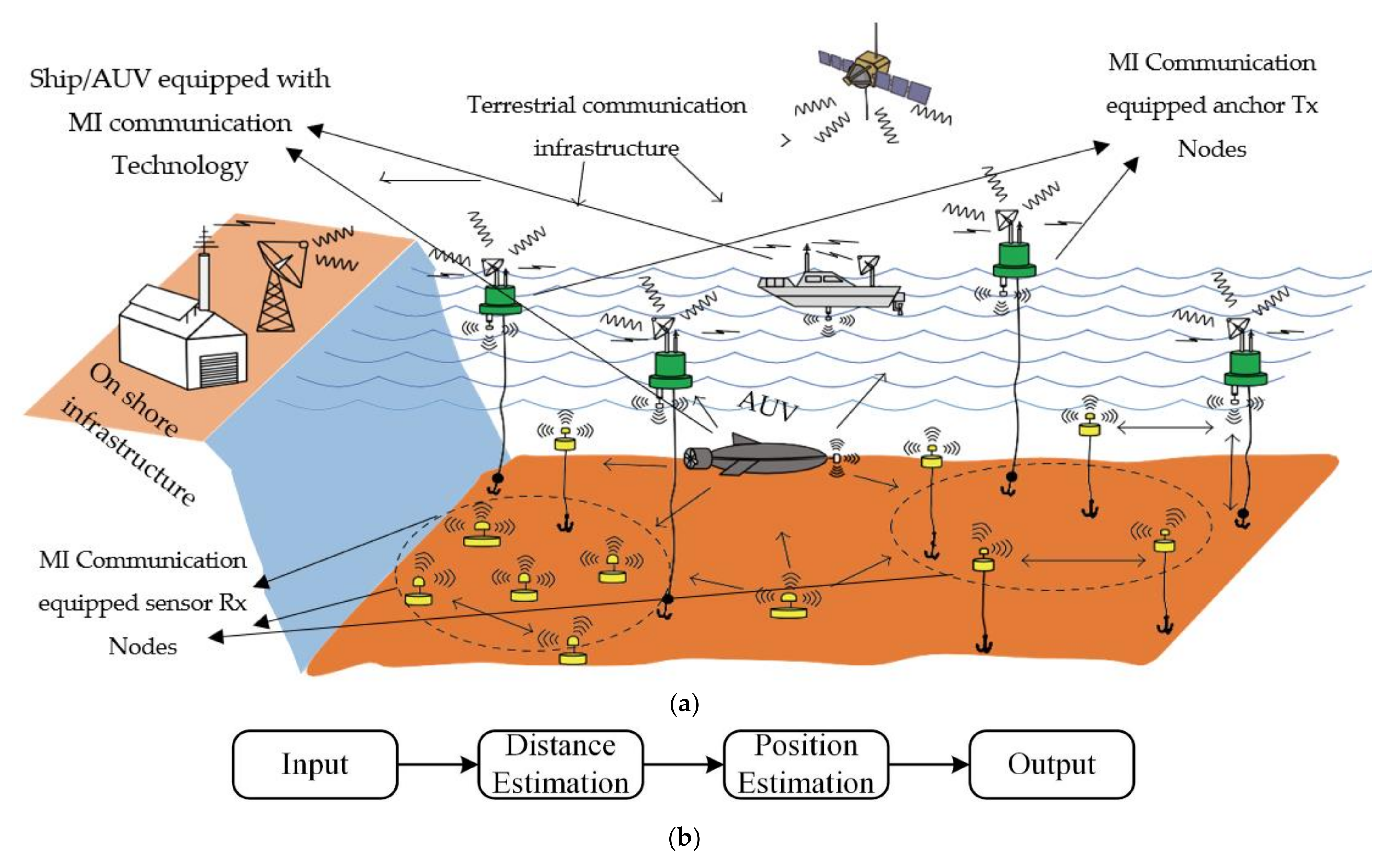
3. Localization and Challenges in MI-UWSNs

In this section, we first briefly present the basic fundamentals of the MI communication, followed by highlighting the directionality challenge in MI communication. This directionality challenge has a significant impact on the range of communication, which directly affects sensor Rx node localization estimation in MI-UWSNs.

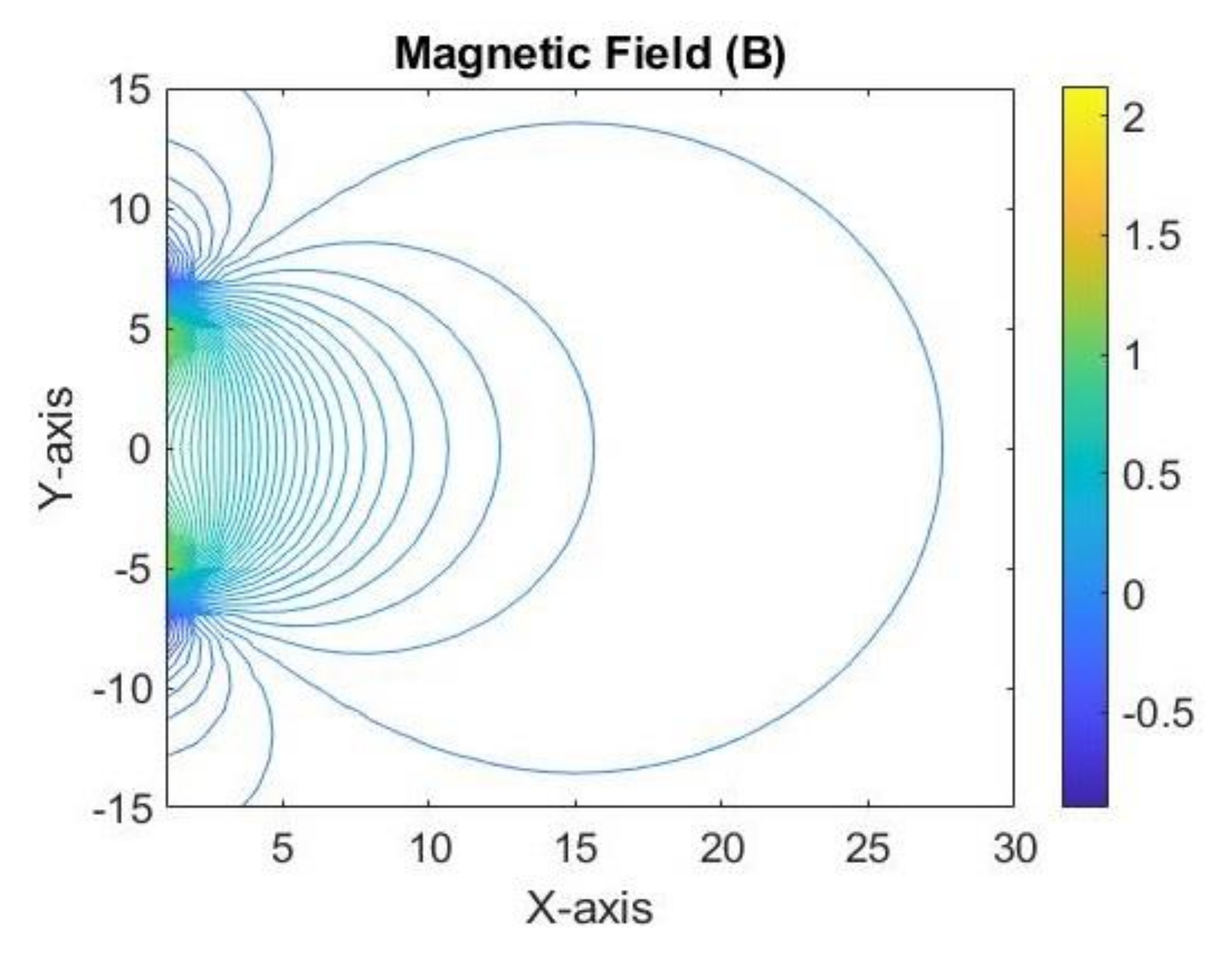
3.1. Physical Nature of Magnetic Fields

To accomplish a point to point MI communication, the MI transmitter (Tx) generates a time-varying magnetic field. The magnetic field produced at the Tx side is given by Equation (11), in which B is the flux along the axis of the current carrying loop $I_t$, ${\mu }_0$ is the permeability of the material, which in our case is the vacuum and has a value of 1, N is the number of turns and is kept the same for both anchor Tx and sensor Rx coils, R is the radius of the current carrying coil, and x is the distance between anchor Tx and sensor Rx coils.

$$B={\mu }_{0}N{I}_t{R}^2/2{\left(x^2+R^2\right)}^{\left(3/2\right)}$$

(11)

The directional magnetic field lines in the xy plane are shown in Figure 2. This magnetic field is quasi-static and therefore behaves differently from a radiative magnetic far-field. Thus, to communicate with the anchor Tx node, the sensor Rx node has to lie inside the magnetic field created by the Tx node. The amount of voltage induced in the Rx node indicates a successful MI communication, and is given by Equation (12).

$$V_{ind}=-\frac{d{\theta }_B}{dt}=2\pi fNBAcos\theta$$

(12)

where ${\theta }_B$ is the magnetic flux density and is calculated by ${\theta }_B$ = BA cos (θ), f is the operating frequency of the applied sinusoidal current, N denotes the number of turns of Tx and Rx coils, A represents the area of the coils, and θ is the angle between the anchor and sensor nodes. Depending on the value of $V_{ind}$, a relation between the Tx and Rx nodes’ distance can be achieved. It can be observed that this relation is strictly dependent on the angle between the communicating nodes, i.e., cos (θ). This relationship highly impacts the robustness of MI communication in UWSNs and hence is very important.

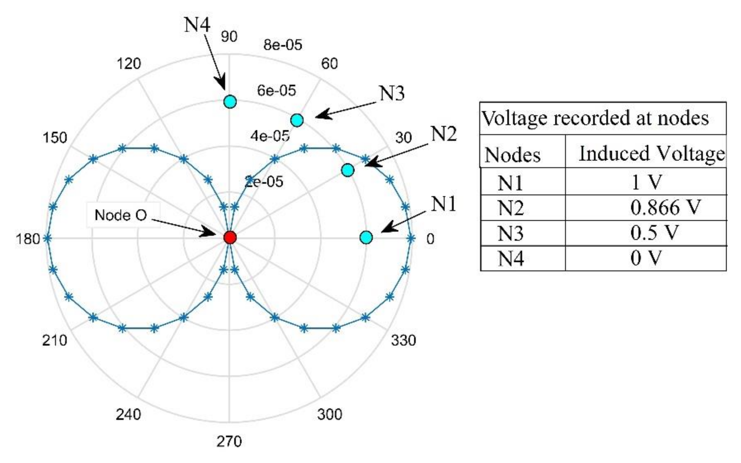
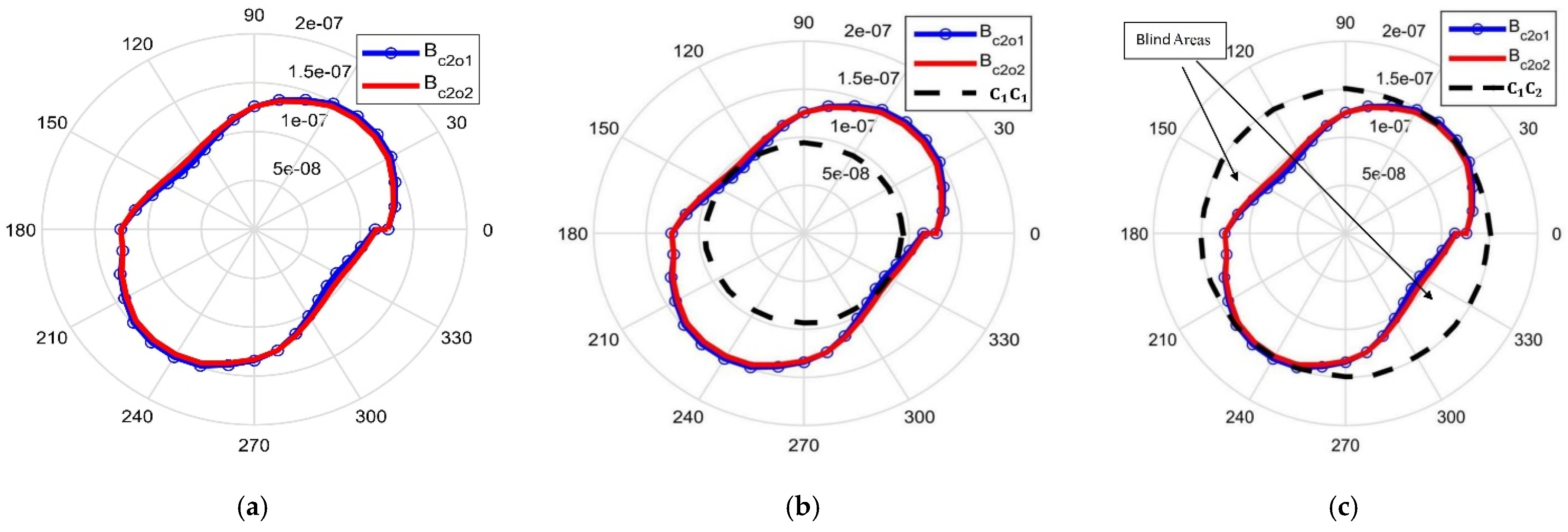
3.2. Highlighting the Directionalilty Problem

The directivity/orientation issue is elaborately in Figure 3, in which four different sensor Rx nodes, i.e., N1, N2, N3, and N4 are placed at a distance of 15 m from the anchor Tx node N0 at an angle of $\theta =0^{°}$, $\theta ={30}^{°}$, $\theta ={60}^{°}$, and $\theta ={90}^{°}$, respectively. It can be observed in Figure 3 that although all Rx nodes are at an equal distance from Tx node, they have different voltages. It can be observed that the maximum voltage is induced when N1 is at $\theta =0^{°}$ with respect to the Tx Node N0, whereas no voltage is induced when N4 is placed at θ = ${90}^{°}$ with respect to the Tx Node. Therefore, the directionality issue poses a significant challenge in designing the RSSI-based localization algorithm to locate any unknown sensor Rx node in MI-UWSNs.

In recent literature, various studies have been reported on the design of multi-dimensional coils (tri-directional (TD) coils and meta-material-based coils) for the Tx and Rx nodes to overcome the directionality challenge posed by the single-dimensional Tx and Rx coils [38,39]. The meta-material-based coils are hard to practically design/implement and therefore these coils are less preferred, whereas TD coils are more preferred because they happen to be low cost, simple, and can easily be re-designed and used. The TD coils can be used in two possible configurations given in Figure 4. We normally have to trade-off between range and power consumption while selecting each configuration.

(1)

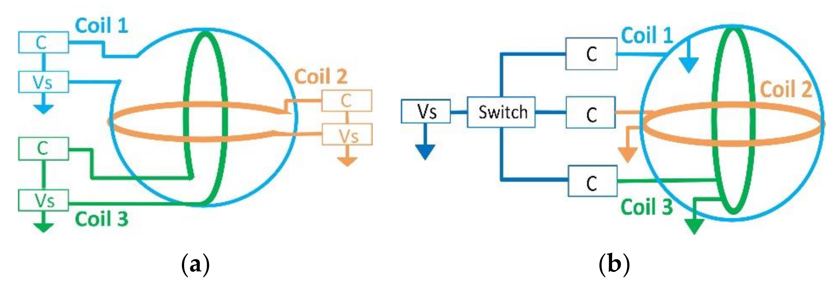
Configuration 1 is a TD coil design, in which each of the three coils are coupled to an independent current source, as shown in Figure 4a. Furthermore, each of the three coils is transmitting a distinct signal in the form of magnetic flux. This configuration offers large-range communication, but at the expense of higher energy consumption [4,20]. In this configuration, two possible patterns of magnetic flux are generated, i.e., $B_{c201}$ and $B_{c202}$, which are shown in Figure 5a. The pattern $B_{c201}$ is generated when an in-phase current passes through the TD coil, on the other hand, the pattern $B_{c202}$ is generated when an out-of-phase current flows through the TD coil.

(2)

The configuration 2 is a TD coil design, in which a switch connects each of the three coils to a single source as shown in Figure 4b, allowing just one coil (along its dimension) to be used at a time. The configuration 2 uses less energy but takes three times longer to transfer data [4,20]. The magnetic flux produced by configuration 2, i.e., $B_{c3}$ is given in Figure 6. The $B_{c3}$ is the combination of the magnetic flux produced by each of the three coils, which is represented by $B_1, B_2,$ and $B_3$, respectively. But here, as the data are presented in an xy plane, therefore, only $B_1 \mathrm{and} B_2$ are shown in Figure 6.

Both these configurations significantly improve the directivity patterns. However, the generated patterns are not completely omnidirectional and have some blind areas, which can be observed in Figure 5c and Figure 6c. Thus, this leads to two further cases for each configuration, which are explained next, in Section 3.3.

3.3. Impact of Directionality on Communication Distance

For robust communication between the Tx and Rx nodes, each of the two configurations described in the previous section can be used independently in any application related to MI-UWSNs. Moreover, in this paper, each configuration has further been divided into two possible cases to investigate the aforementioned configurations in detail. The possible cases that have been investigated for configuration 1 and 2 are shown in Figure 5 and Figure 6, respectively.

3.3.1. Possible Cases of Configuration 1

The two possible cases for configuration 1, i.e., $C_1{C}_1$ and $C_1{C}_2$, are shown in Figure 5b,c, respectively. In configuration 1 case 1 ($C_1{C}_1$) shown in Figure 5b, it can be observed that a 360° communication is achieved but with an obvious decrease in the communication radius. If this region is used for communication, an increased number of Tx nodes will be required to locate a Rx node in the given area. Similarly, in the case of Figure 5c, i.e., the configuration 1 case 2 ($C_1{C}_2)$, a larger area can be localized, but with blind areas from ${80}^{°}$ to ${200}^{°}$ and ${270}^{°}$ to ${20}^{°}$, which in total combine to form ${120}^{°}$ + ${110}^{°}$ = ${230}^{°}$ of blind areas. If the $C_1{C}_2$ case is utilized, there will be no communication in these 230° s of blind areas, which are mentioned in Figure 5c. Hence, in the $C_1{C}_2$ case, there will be a high probability of localization inaccuracy that must be assessed in order to determine its impact on the localization estimation of a node in MI-UWSNs.

3.3.2. Possible Cases of Configuration 2

The two possible cases for configuration 2, i.e., $C_2{C}_1$ and $C_2{C}_2$ are shown in Figure 6b,c, respectively. In configuration 2 case 1 ($C_2{C}_1$), as shown in Figure 6b, it can be observed that a 360° communication is achieved but with an obvious decrease in communication radius. If this region is used for communication, an increased number of Tx nodes will be required to locate a Rx node in the given area. Similarly, in case of Figure 6c, i.e., the configuration 2 case 2 ($C_2{C}_2)$, a larger area can be localized, but with blind areas from ${110}^{°}$ to ${160}^{°}$, ${210}^{°}$ to ${260}^{°}$, ${290}^{°}$ to ${350}^{°}$, and ${20}^{°}$ to ${70}^{°}$, which in total combines to form ${200}^{°}$ s of blind areas. If the $C_2{C}_2$ case is utilized, there will be no communication in these 200° s of blind areas, which are mentioned in Figure 6c. Hence, in the $C_2{C}_2$ case, there will be a high probability of localization inaccuracy that must be assessed in order to determine its impact on the localization estimation of a node in MI-UWSNs.

From the possible cases of configuration 1 and 2 described above, it can be inferred that the range of MI communication can be increased by increasing the power provided to the Tx node. However, the power should only be increased to a limit where it would not drain the power source of the Tx node. Furthermore, the increase in current could also lead to the melting of the lamination around the inductor, which in turn can short-circuit the entire coil. This short circuit would draw an additional current from the system and can damage the fuse or the coil itself. In addition, a damaged coil will result in the loss of a node in a cooperative MI-UWSN, which could delay the data to be received at the Rx end. For these aforementioned reasons, the two possible configurations have been taken into account. If we require fast data transmission and there is no cap on the energy requirement, then the configuration 1 is most suitable. On the other hand, if the requirement focuses on low energy consumption and the speed of data transmission can be compromised, then configuration 2 is the most suitable option.

4. Evaluation of Localization Scheme

4.1. Evaluation Setup

Keeping in mind the impact of blind areas in MI communication between Tx and Rx nodes, a simulation environment of 15 m × 15 m has been created, in which a minimum of two and a maximum of eight Tx nodes have been utilized to initiate the process of the localization of nodes in a MI-UWSN. The localization process was initiated by localizing one Rx node with two Tx nodes, gradually increasing the number of Tx nodes to eight. To evaluate the accuracy of our localization algorithm, the number of Rx nodes were gradually increased from one to eight after establishing a stable environment.

4.1.1. The Localization Process

To elaborate upon the localization estimation results for the Rx nodes in a 15 m × 15 m realm, a simulation environment was generated on MATLAB, in which Tx node positions were set at locations A(0, 0), B(15, 15), C(0, 15), D(15, 0) and E(15, 7.5), F (7.5, 15), G(0, 7.5), and H(7.5, 0). Furthermore, to measure the localization error, the Rx nodes are plotted randomly each time the simulation is run. Before calculating the location of the Rx nodes, we incorporated the errors in the localization algorithm, induced by the blind areas discussed in Section 3.3.1 and Section 3.3.2. This is performed to estimate the amount of localization estimation errors faced when the system is implemented in a real-world scenario. The Euclidean distances between the Tx and Rx nodes were then calculated using Equation (13). Finally, the Gauss–Newton method was used to find the minimum of the Euclidean distances by using Equation (14), which represents our localization estimation.

$$d\left(x,y\right)=\sqrt{{\displaystyle \sum }_{i=1}^n{\left(x_i+y_i\right)}^2}$$

(13)

$$\left|\right|f_x|{|}_2^2={\displaystyle \sum }_{i=1}^{m}fi{(x)}^2$$

(14)

The process of localization, as shown in Figure 7, starts with the known locations of Tx nodes; the next step is to localize the unknown Rx nodes. The current provided to the Tx nodes results in the generation of magnetic flux, which in turn induces a voltage in the Rx nodes. This induced voltage represents the distance between the Rx and Tx nodes. A threshold value has been set in the algorithm for this induced voltage. When the value of induced voltage is above this threshold point, the algorithm confirms that the Rx node is in the communication range, which is depicted in Figure 5c and Figure 6c. In addition, if the Rx and Tx nodes are communicating as shown in Figure 5b and Figure 6b, a high localization accuracy is obtained. On the other hand, if Rx nodes are on the boundary of the communication radius mentioned in Figure 5c and Figure 6c, a low localization accuracy is obtained. This localization estimation analysis furthers the underwater-communication field by helping the researchers to implement the real-life/practical prototypes of MI-UWSNs.

To understand and reproduce the results analyzed in this study, a pseudo code of the opted algorithm is given below in Section 4.1.2.

4.1.2. Pseudo Code of the Proposed Methodology

For the ease of the readers who want to reproduce the results that are addressed in this study, a pseudo code as Algorithm 1 is provided in this section. As a first step, we provided the number of anchor Tx nodes that are used for the localization estimation at known positions, and the number of sensor Rx nodes that are to be localized. Rx nodes are deployed randomly in a 15 m × 15 m simulation environment in MATLAB for every iteration. Once the environment was set up for localization, the distance between the Tx and Rx node is calculated. The loop will be executed until all the iterations are completed and once we get all the Euclidian distances between Tx and Rx nodes. In the next step we had to add the inaccuracies caused by the directionality factor explained in detail in Section 3. Then, we applied the Gauss–Newton method to find the minimum of all the obtained functions from the calculation of Euclidean distances. At the end, a mean square error is calculated, which is basically the difference between the Rx node location estimation and its original location.

Algorithm 1: A Pseudo Code of the Proposed Methodology

Start

:  N = number of anchor Tx nodes

:  M = number of sensor Rx nodes

:  Error due to directionality = %

:  Network size = 15 m × 15 m

:  Computing the Euclidian distance b/w nodes

:  for m = 1:M

:  :  for n = 1:N

:  :  :  distance(n,m) = sqrt(anchor(n,1)-sensor(m,1))^2

:  :  end

:  end

::  Noise calculation = distance + distance. × Error due to directionality

::  Location Estimation = network Size × rand(M,2)

:  for m = 1:M

:  :     for i = 1:number of Iteration

:  :     end

:  end

:  $\mathrm{Err}=\mathrm{mean}(\sqrt{\left(\mathrm{sum}\left(\left(\mathrm{mobileLocationEstimation}-\mathrm{mobileLocation}\right).^2\right)\right)}$)

End

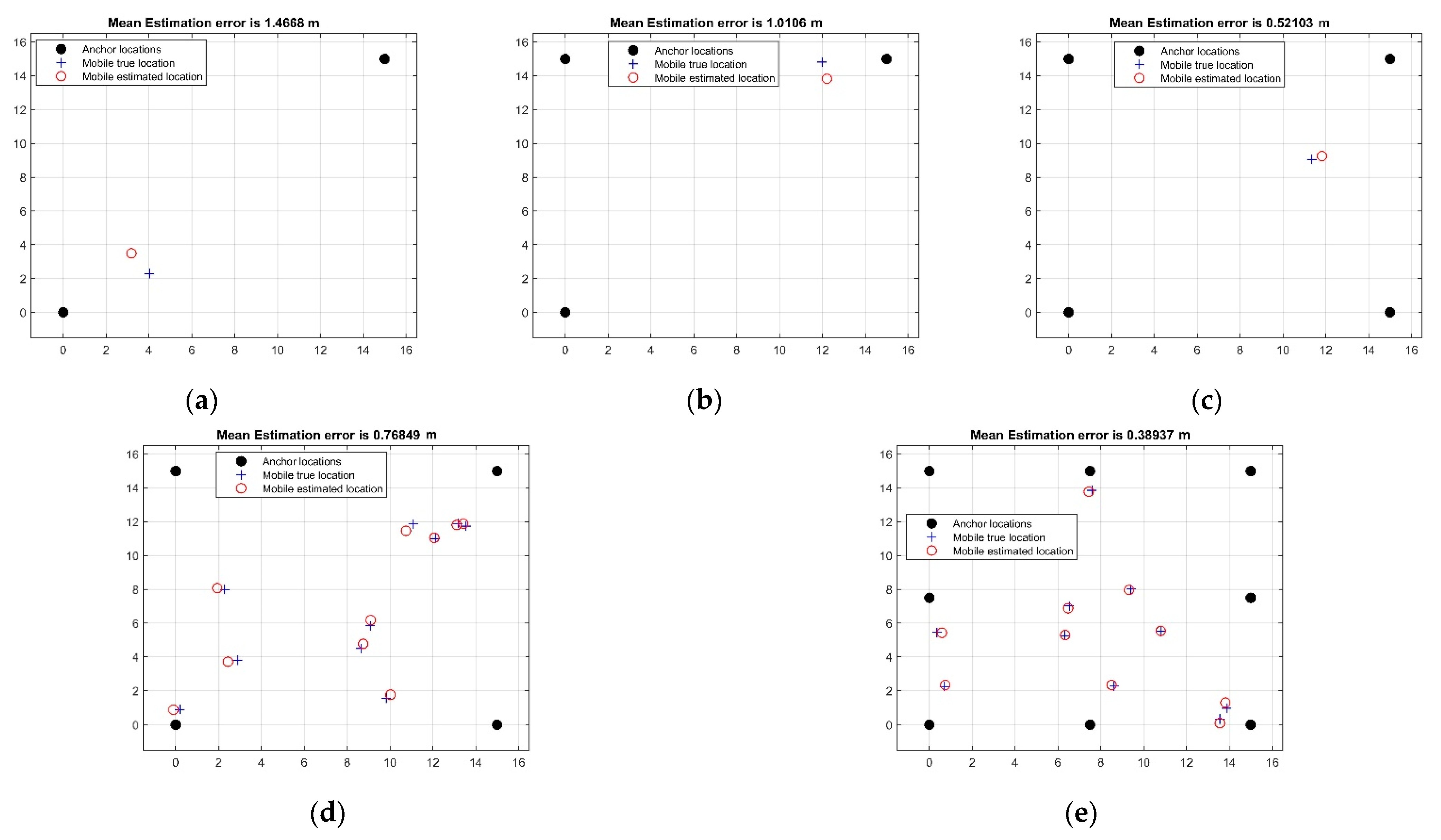
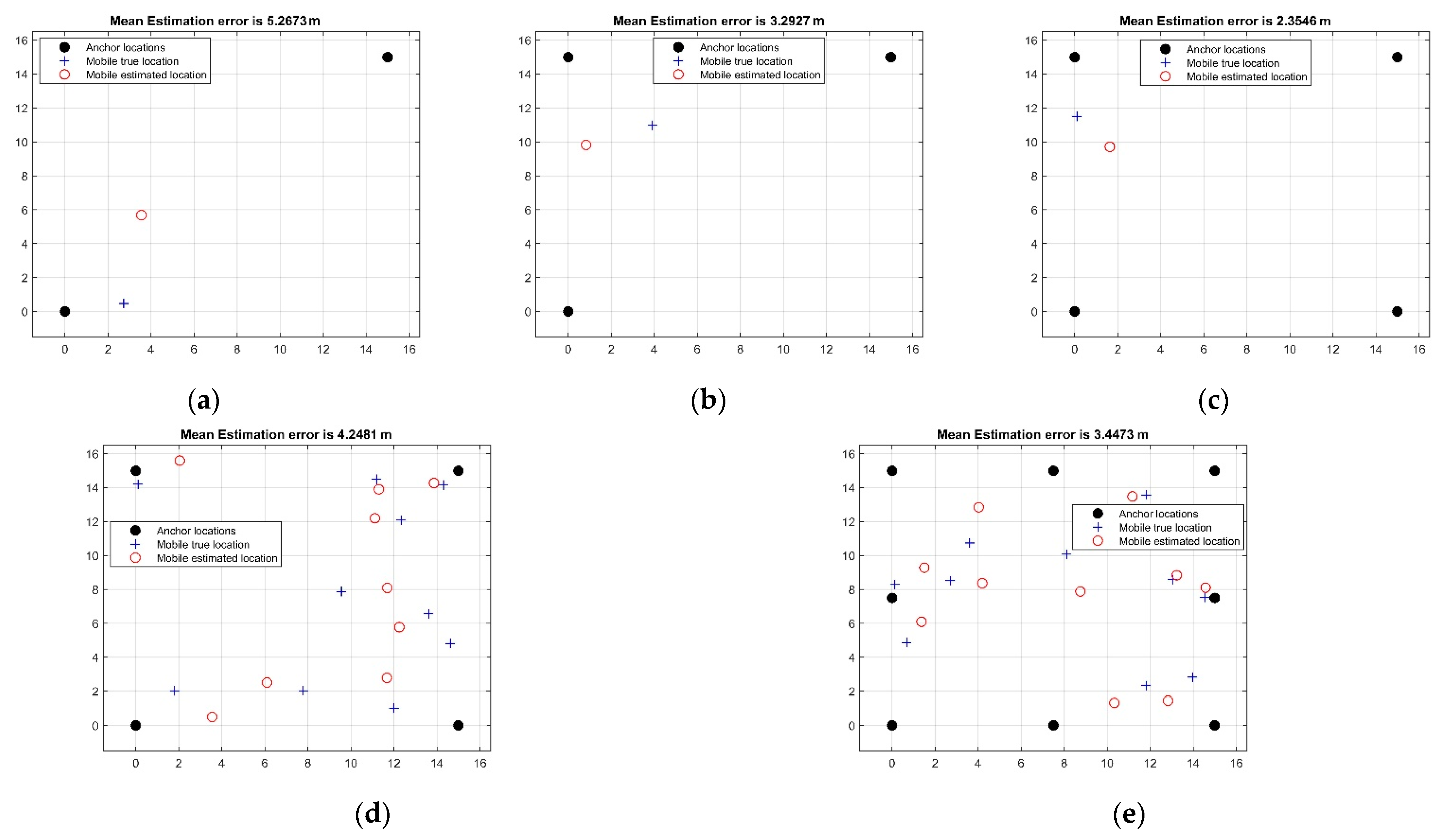
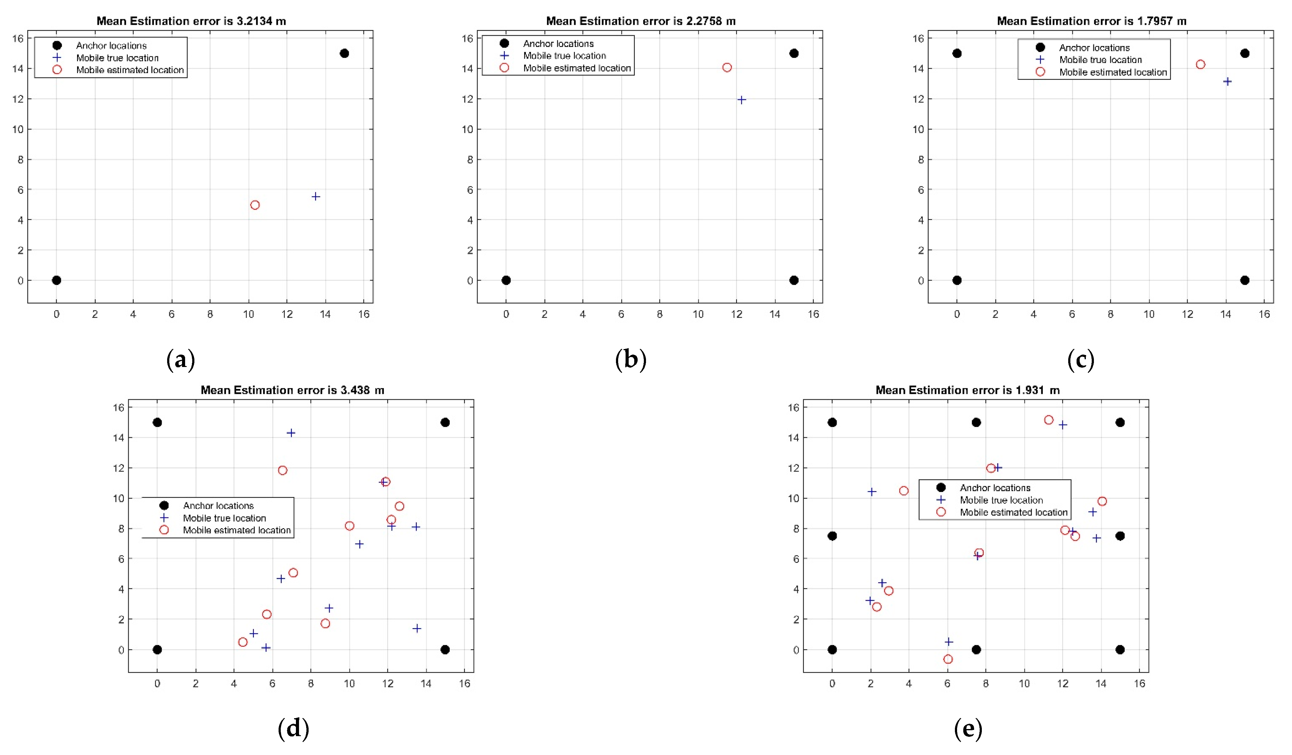
4.2. Results of Localization Estimation

4.2.1. Effect of Blind Areas with Configuration 1 Case 1

Presently, taking into consideration the communication of configuration 1 case 1 ($C_1{C}_1$) depicted in Figure 5b, the localization estimation results are obtained for an omni-directional scenario in a 15 m × 15 m simulation environment using the MI communication. It can be observed in Figure 8a that the two Tx nodes at location A(0, 0) and B(15, 15) are used to localize a single Rx node, which give an estimation accuracy of 90.26%. In addition, in Figure 8b, three Tx nodes at location A(0, 0), B(15, 15), and C(0, 15) are used, which give an estimation accuracy of 93.26%. Similarly, in Figure 8c, four Tx nodes at location A(0, 0), B(15, 15), C(0, 15), and D(15, 0) are used, which give an estimation accuracy of 96.53%. It is evident from Figure 8a–c that as the number of Tx nodes increase, the estimation accuracy is improved. This dependency of the improvement in the estimation accuracy on the number of Tx nodes is shown in Figure 8d,e. It can be observed in Figure 8d that for only four Tx nodes, when the number of Rx nodes is increased to 10, the estimation accuracy drops to 94.93%. However, in Figure 8e, when the number of Tx nodes is increased to eight (at location A(0, 0), B(15, 15), C(0, 15), D(15, 0) and E(15, 7.5), F(7.5, 15), G(0, 7.5), H(7.5, 0)), the estimation accuracy improves to 97.46%.

4.2.2. Effect of Blind Areas with Configuration 1 Case 2

Taking into consideration the configuration 1 case 2 ($C_1{C}_2$) presented in Figure 5c, the localization radius of sensor Rx nodes denoted by $C_1{C}_2$ is increased, but the RSSI denoted by $B_{C201}$ and $B_{C202}$ has been kept same. The directivity of MI communication plays an important role in this case. Figure 5c shows the blind areas from ${80}^{°}$ to ${200}^{°}$ and ${270}^{°}$ to ${20}^{°}$, which in total combine to form ${120}^{°}$ + ${110}^{°}$ = ${230}^{°}$. These ${230}^{°}$ s out of ${360}^{°}$ s in total are the directional point where no MI communication is taking place. Therefore, it can be concluded from Equation (15) that 63.8% of the total communication radius, which is formed by the combination of $B_{C202}$ and $B_{C201}$, represents the localization estimation error. Hence, we only have 36.2% accuracy while localizing a sensor Rx node using MI communication in a UWSN.

$$\frac{{230}^{°}\times 100}{{360}^{°}}=63.8\%$$

(15)

To cater the directionality factor in MI communication, the accuracy obtained from Equation (15) is incorporated in the localization algorithm and the localization estimation results shown in Figure 9a–e are obtained. In Figure 9a, two anchor nodes at location A(0, 0) and B(15, 15) are used to localize one Rx node, for which we obtained the localization estimation accuracy of 65.3%. In addition, in Figure 9b, three Tx nodes at location A(0, 0), B(15, 15), and C(0, 15) are used, which give an estimation accuracy of 78.06%. Similarly, in Figure 9c, 4 Tx nodes at location A(0, 0), B(15, 15), C(0, 15), and D(15, 0) are used, which give an estimation accuracy of 84.3%. It is evident from Figure 9a–c that as the number of Tx nodes increases, the estimation accuracy is improved. This dependency of the improvement in the estimation accuracy on the number of Tx nodes is shown in Figure 9d,e. It can be observed in Figure 9d that for only four Tx nodes, when the number of Rx nodes is increased to 10, the estimation accuracy drops to 71.46%. However, in Figure 9e, when the number of Tx nodes is increased to eight (at location A(0, 0), B(15, 15), C(0, 15), D(15, 0) and E(15, 7.5), F(7.5, 15), G(0, 7.5), and H(7.5, 0)), the estimation accuracy improves to 77.06%.

4.2.3. Effect of Blind Areas with Configuration 2 Case 1

Now taking into consideration the communication configuration 2 case 1 ($C_2{C}_1$) depicted in Figure 6b, the localization estimation results are obtained for an omni-directional scenario in a 15 m × 15 m simulation environment using the MI communication. It can be observed in Figure 8a that the two Tx nodes at location A(0, 0) and B(15, 15) are used to localize a single Rx node, which gives an estimation accuracy of 90.26%. In addition, in Figure 8b, three Tx nodes at location A(0, 0), B(15, 15), and C(0, 15) are used, which give an estimation accuracy of 93.26%. Similarly, in Figure 8c, four Tx nodes at location A(0, 0), B(15, 15), C(0, 15), and D(15, 0) are used, which give an estimation accuracy of 96.53%. It is evident from Figure 8a–c that as the number of Tx nodes is increased, the estimation accuracy is improved. This dependency of the improvement in the estimation accuracy on the number of Tx nodes is shown in Figure 8d,e. It can be observed in Figure 8d that for only four Tx nodes, when the number of Rx nodes is increased to 10, the estimation accuracy drops to 94.93%. However, in Figure 8e, when the number of Tx nodes is increased to eight (at location A(0, 0), B(15, 15), C(0, 15), D(15, 0) and E(15, 7.5), F(7.5, 15), G(0, 7.5), and H(7.5, 0)), the estimation accuracy improves to 97.46%.

4.2.4. Effect of Blind Areas with Configuration 2 Case 2

Taking into consideration the configuration 2 case 2 ($C_2{C}_2$) presented in Figure 6c, there are blind areas for MI communication from ${110}^{°}$ to ${160}^0$, ${210}^{°}$ to ${260}^{°}$, ${290}^{°}$ to ${350}^{°},$ and ${20}^{°}$ to ${70}^{°},$ summing up to ${200}^{°}$ s. These ${200}^{°}$ s out of ${360}^{°}$ s in total are the directional points on the communication radius $C_2{C}_2$, where no MI communication takes place. From Equation (16), it can be concluded that 55.5% of the total communication radius in Figure 6c is the estimation error in localization while considering $C_2{C}_2$, which means that we are left with only 44.5% accuracy while localizing a sensor node using MI communication. This is an increase in the localization estimation accuracy in comparison with the configuration, as discussed earlier in Section 4.2.2

$$\frac{{200}^{°}\times 100}{{360}^{\mathrm{°}}} = 55.5\%$$

(16)

To cater the directionality factor in MI communication, the accuracy obtained from Equation (16) is incorporated in the localization algorithm, and the localization estimation results shown in Figure 10a–e are obtained. In Figure 10a, two anchor nodes at location A(0, 0) and B(15, 15) are used to localize one Rx node, for which we obtained the localization estimation accuracy of 78.6%. In addition, in Figure 10b, three Tx nodes at location A(0, 0), B(15, 15), and C(0, 15) are used, which give an estimation accuracy of 84.86%. Similarly, in Figure 10c, four Tx nodes at location A(0, 0), B(15, 15), C(0, 15), and D(15, 0) are used, which give an estimation accuracy of 88.06%. It is evident from Figure 10a–c that as the number of Tx nodes is increased, the estimation accuracy is improved. This dependency of the improvement in the estimation accuracy on the number of Tx nodes is shown in Figure 10d,e. It can be observed in Figure 10d that for only four Tx nodes, when the number of Rx nodes is increased to 10, the estimation accuracy drops to 77.13%. However, in Figure 10e, when the number of Tx nodes is increased to eight (at location A(0, 0), B(15, 15), C(0, 15), D(15, 0) and E(15, 7.5), F(7.5, 15), G(0, 7.5), and H(7.5, 0)), the estimation accuracy improves to 87.13%.

5. Comparison and Summary

It is possible to display all results of localization estimation graphically; however, it will be quite difficult for readers to go through 210 graphs simultaneously. Hence, all results have been quantified and summarized in

Table 2. Comparative analysis of localization estimation results.

S. No	Number of Tx Nodes	1 Rx Node	2 Rx Node	3 Rx Node	4 Rx Node	5 Rx Node	6 Rx Node	7 Rx Node	8 Rx Node	9 Rx Node	10 Rx Node
1	2Tx nodes ((C_1C_1)(C_2C_1))	90.26%	89.4%	88.2%	86.8%	83.33%	81.66%	80.13%	79.2%	77.3%	76.86%
2	2Tx nodes (C_1C_2)	65.3%	64.6%	61.67%	60.73%	59%	56.26%	53.66%	52.86%	52.2%	51.6%
3	2Tx nodes (C_2C_2)	78.6%	77.6%	76.26%	75%	73.73%	72.46%	70.93%	72.2%	66.6%	64.86%
4	3Tx nodes ((C_1C_1)(C_2C_1))	93.26%	91.8%	91%	90.73%	90.06%	88.3%	87.4%	87%	86.53%	85.8%
5	3Tx nodes (C_1C_2)	78.6%	77.5%	76.86%	76.06%	75%	74.2%	71.6%	69.6%	68.13%	66.8%
6	3Tx nodes (C_2C_2)	82%	84.73%	83.6%	83.26%	82.46%	81.6%	80.73%	80.26%	79.93%	79.13%
7	4Tx nodes ((C_1C_1)(C_2C_1))	96.53%	96.26%	96.06%	95.8%	95.6%	95.4%	95.26%	95.2%	95.06%	94.93%
8	4Tx nodes (C_1C_2)	84.6%	84.2%	83.6%	80.46%	79.13%	76.26%	74.73%	73.53%	72.6%	71.73%
9	4Tx nodes (C_2C_2)	88.6%	87.26%	86%	84%	82%	8.53%	79.13%	78.26%	77.53%	77.3%
10	8Tx nodes ((C_1C_1)(C_2C_1))	99.2%	98.86%	98.6%	98.26%	98.06%	97.93%	97.73%	97.6%	97.53%	97.46%
11	8Tx nodes (C_1C_2)	89.53%	89.13%	88.6%	87.86%	84.86%	82.93%	80.93%	80.06%	78.46%	77.06%
12	8Tx nodes (C_2C_2)	90.04%	89.93%	89.53%	89.2%	88.6%	88.06%	87.86%	87.46%	87.26%	87.13%

, where the results of $C_1{C}_1$ and $C_2{C}_1$ have been combined because they both depict omni-directionality as explained earlier in Section 4.2.1 and Section 4.2.3. It can be observed that as we increase the number of anchor Tx nodes to localize sensor Rx nodes, the estimation results for localization improve gradually. Similarly, the same incremental process in anchor Tx nodes is opted for $C_1{C}_2$ and $C_2{C}_2$. However, the results will change depending on the amount of area in which communication cannot be performed, which is referred to as blind areas in MI-UWSNs.

6. Conclusions

In this paper, the directionality issue in MI-UWSNs while localizing the sensor Rx nodes has been addressed. For this purpose, a RSSI-based multilateration localization algorithm has been proposed and evaluated. Furthermore, this paper highlights and presents the role of blind areas in the accurate localization of Rx nodes. For the accurate estimation of the sensor nodes’ location, the blind areas in the tri-dimensional coil designs have also been calculated and incorporated in the proposed algorithm. For the two presented cases of blind areas, i.e., $C_1{C}_2$, and $C_2{C}_2$, an estimation accuracy of 77.06%, and 87.13% is achieved, respectively. To the authors’ knowledge, the impact of blind areas on the localization accuracy has never been considered and evaluated before. Furthermore, from the localization estimation analysis, it is concluded that an increase in the number of Tx nodes results in improved localization estimation accuracy; on the other hand, an increase in the Rx nodes results in the reduction of estimation accuracy. The results indicate that for an increase in the anchor Tx nodes from two to eight, the localization estimation accuracy increased from 65.3% to 89.53% for case $C_1{C}_2$, and from 78.6% to 90.04% for case $C_2{C}_2$. On the other hand, for an increase in the sensor Rx nodes from 1 to 10, the localization estimation accuracy dropped from 89.53% to 77.06% for case $C_1{C}_2$, and from 90.04% to 87.13% for case $C_2{C}_2$.

There are some limitations of the MI technology that need to be addressed before deploying such a system in UWSNs: (1) It is a near field of communication, thus long-distance communication is not possible. (2) The presence of ferromagnetic materials in the environment will affect the MI communication, which in turn will lower the accuracy of estimating the position of sensor Rx nodes. Phenomenon such as refraction, scattering, and multi-paths attributed to the prevalence of unforeseen challenges and limited visibility, which make it difficult to communicate in UWSNs. It is an advantage in MI communication that it is not affected by the aforementioned phenomenon. For future work, our research team is trying to build a machine learning-based linear regression model to predict the location of a sensor Rx node in MI-UWSNs.

References

1. Felemban, E.; Shaikh, F.K.; Qureshi, U.M.; Sheikh, A.A.; Qaisar, S.B. Underwater sensor network applications: A comprehensive survey. Int. J. Distrib. Sens. Netw. 2015, 11, 896832. [Google Scholar] [CrossRef] [Green Version]
2. Alrajeh, N.A.; Bashir, M.; Shams, B.J. Localization techniques in wireless sensor networks. Int. J. Distrib. Sens. Netw. 2013, 9, 304628. [Google Scholar] [CrossRef] [Green Version]
3. Raghavendra, C.S.; Sivalingam, K.M.; Znati, T. Wireless Sensor Networks; Springer: Berlin/Heidelberg, Germany, 2006. [Google Scholar]
4. Muzzammil, M.; Ahmed, N.; Qiao, G.; Ullah, I.; Wan, L. Fundamentals and advancements of magnetic-field communication for underwater wireless sensor networks. IEEE Trans. Antennas Propag. 2020, 68, 7555–7570. [Google Scholar] [CrossRef]
5. Singh, S.P.; Sharma, S.C. Range free localization techniques in wireless sensor networks: A review. Procedia Comput. Sci. 2015, 57, 7–16. [Google Scholar] [CrossRef] [Green Version]
6. He, T.; Huang, C.; Blum, B.M.; Stankovic, J.A.; Abdelzaher, T. Range-free localization schemes for large scale sensor networks. In Proceedings of the 9th Annual International Conference on Mobile Computing and Networking, Diego, CA, USA, 14–19 September 2003; pp. 81–95. [Google Scholar]
7. He, T.; Huang, C.; Blum, B.; Stankovic, J.; Abdelzaher, T. Range-free localization and its impact on large scale sensor networks. ACM Trans. Embed. Comput. Syst. 2005, 4, 877–906. [Google Scholar] [CrossRef]
8. Manzoor, R. Energy efficient localization in wireless sensor networks using noisy measurements. Record 2010, 2010, 827–831. [Google Scholar]
9. Stoleru, R.; He, T.; Stankovic, S. Secure Localization and Time Synchronization for Wireless Sensor and Ad Hoc Networks; Range-Free Localization Advance Information Security Series; Springer Science & Business Media: Berlin/Heidelberg, Germany, 2007; Volume 30. [Google Scholar]
10. Zhang, Y.; Wu, W.; Chen, Y. A range-based localization algorithm for wireless sensor networks. J. Commun. Netw. 2005, 7, 429–437. [Google Scholar] [CrossRef]
11. Almuzaini, K.K.; Gulliver, A. Range-based localization in wireless networks using density-based outlier detection. Wirel. Sens. Netw. 2010, 2, 807. [Google Scholar] [CrossRef] [Green Version]
12. Mekelleche, F.; Haffaf, H. Classification and Comparison of Range-Based Localization Techniques in Wireless Sensor Networks. J. Commun. 2017, 12, 221–227. [Google Scholar] [CrossRef] [Green Version]
13. Zanca, G.; Zorzi, F.; Zanella, A.; Zorzi, M. Experimental comparison of RSSI-based localization algorithms for indoor wireless sensor networks. In Proceedings of the Workshop on Real-World Wireless Sensor Networks, Glasgow, Scotland, 1 April 2008; pp. 1–5. [Google Scholar]
14. Abrudan, T.E.; Xiao, Z.; Markham, A.; Trigoni, N.; Sensing, R. Underground incrementally deployed magneto-inductive 3-D positioning network. IEEE Trans. Geosci. 2016, 54, 4376–4391. [Google Scholar] [CrossRef]
15. Markham, A.; Trigoni, N.; Macdonald, D.W.; Ellwood, S.A. Underground localization in 3-D using magneto-inductive tracking. IEEE Sens. J. 2011, 12, 1809–1816. [Google Scholar] [CrossRef] [Green Version]
16. Huang, H.; Zheng, Y.R. Node localization in 3-D by magnetic-induction communications in wireless sensor networks. In Proceedings of the OCEANS 2017-Anchorage, Anchorage, AK, USA, 18–21 September 2017; pp. 1–6. [Google Scholar]
17. Wahlström, J.; Kok, M.; de Gusmao, P.P.B.; Abrudan, T.E.; Trigoni, N.; Markham, A. Sensor fusion for magneto-inductive navigation. IEEE Sens. J. 2019, 20, 386–396. [Google Scholar] [CrossRef] [Green Version]
18. Baffelli, S. Localization of Low Complexity Communication Devices Based on Mutual Inductive Coupling. Master’s Thesis, Communication Technology Laboratory Wireless Communications Group, Swiss Fedral Institute of Technology, Zurich, Switzerland, 2013. [Google Scholar]
19. Tan, X.; Sun, Z.; Wang, P.; Sun, Y. Environment-aware localization for wireless sensor networks using magnetic induction. Ad Hoc Netw. 2020, 98, 102030. [Google Scholar] [CrossRef]
20. Ahmed, N.; Radchenko, A.; Pommerenke, D.; Zheng, Y.R. Design and evaluation of low-cost and energy-efficient magneto-inductive sensor nodes for wireless sensor networks. IEEE Syst. J. 2018, 13, 1135–1144. [Google Scholar] [CrossRef]
21. Gaoding, N.; Bousquet, J.-F. A compact magneto-inductive coil antenna design for underwater communications. In Proceedings of the International Conference on Underwater Networks & Systems, Halifax, NS, Canada, 6–8 November 2017; pp. 1–5. [Google Scholar]
22. Huang, H.; Zheng, Y.R. 3-D localization of wireless sensor nodes using near-field magnetic-induction communications. Phys. Commun. 2018, 30, 97–106. [Google Scholar] [CrossRef]
23. Yabukami, S.; Kikuchi, H.; Yamaguchi, M.; Arai, K.; Takahashi, K.; Itagaki, A.; Wako, N. Motion capture system of magnetic markers using three-axial magnetic field sensor. IEEE Trans. Magn. 2000, 36, 3646–3648. [Google Scholar] [CrossRef]
24. Hu, C.; Meng, M.Q.-H.; Mandal, M. The calibration of 3-axis magnetic sensor array system for tracking wireless capsule endoscope. In Proceedings of the 2006 IEEE/RSJ International Conference on Intelligent Robots and Systems, Beijing, China, 9–15 October 2006; pp. 162–167. [Google Scholar]
25. Hu, C.; Meng, M.Q.-H.; Mandal, M. A linear algorithm for tracing magnet position and orientation by using three-axis magnetic sensors. IEEE Trans. Magn. 2007, 43, 4096–4101. [Google Scholar]
26. Schlageter, V.; Besse, P.-A.; Popovic, R.; Kucera, P. Tracking system with five degrees of freedom using a 2D-array of Hall sensors and a permanent magnet. Sens. Actuators A Phys. 2001, 92, 37–42. [Google Scholar] [CrossRef]
27. Hu, C.; Song, S.; Wang, X.; Meng, M.Q.-H.; Li, B. A novel positioning and orientation system based on three-axis magnetic coils. IEEE Trans. Magn. 2012, 48, 2211–2219. [Google Scholar] [CrossRef]
28. Hu, C.; Meng, M.Q.-H.; Song, S.; Dai, H. A six-dimensional magnetic localization algorithm for a rectangular magnet objective based on a particle swarm optimizer. IEEE Trans. Magn. 2009, 45, 3092–3099. [Google Scholar]
29. Song, S.; Hu, C.; Li, M.; Yang, W.; Meng, M.Q.-H. Real time algorithm for magnet’s localization in capsule endoscope. In Proceedings of the 2009 IEEE International Conference on Automation and Logistics, Shenyang, China, 5–7 August 2009; pp. 2030–2035. [Google Scholar]
30. Raab, F.H.; Blood, E.B.; Steiner, T.O.; Jones, H.R. Magnetic position and orientation tracking system. IEEE Trans. Aerosp. Electron. Syst. 1979, 5, 709–718. [Google Scholar] [CrossRef]
31. Paperno, E.; Sasada, I.; Leonovich, E. A new method for magnetic position and orientation tracking. IEEE Trans. Magn. 2001, 37, 1938–1940. [Google Scholar] [CrossRef]
32. Fujieda, M.; Tateno, H.; Nara, T.; Hashimoto, M. Discrete Fourier coil for localization of a magnetic dipole. In Proceedings of the SICE Annual Conference, Tokyo, Japan, 13–18 September 2011; pp. 2345–2349. [Google Scholar]
33. Nara, T.; Takanashi, Y.; Watanabe, H. Two-dimensional localization of a magnetic dipole from its first order Fourier coefficients of the magnetic flux density. In Proceedings of the SICE Annual Conference, Taipei, Taiwan, 18–21 August 2010; pp. 3219–3222. [Google Scholar]
34. Nara, T.; Takanashi, Y.; Mizuide, M. A sensor measuring the Fourier coefficients of the magnetic flux density for pipe crack detection using the magnetic flux leakage method. J. Appl. Phys. 2011, 109, 07E305. [Google Scholar] [CrossRef]
35. Caffey, T.W.; Romero, L. Locating a buried magnetic dipole. IEEE Trans. Geosci. Remote Sens. 1982, 2, 188–192. [Google Scholar] [CrossRef]
36. Andrä, W.; Danan, H.; Kirmße, W.; Kramer, H.-H.; Saupe, P.; Schmieg, R.; Bellemann, M.E. A novel method for real-time magnetic marker monitoring in the gastrointestinal tract. Phys. Med. Biol. 2000, 45, 3081–3093. [Google Scholar] [CrossRef] [PubMed]
37. Hashi, S.; Yabukami, S.; Kanetaka, H.; Ishiyama, K.; Arai, K.I. Wireless magnetic position-sensing system using optimized pickup coils for higher accuracy. IEEE Trans. Magn. 2011, 47, 3542–3545. [Google Scholar] [CrossRef]
38. Guo, H.; Sun, Z. M2I communication: From theoretical modeling to practical design. In Proceedings of the 2016 IEEE International Conference on Communications (ICC), Kuala, Lumpur, 23–27 May 2016; pp. 1–6. [Google Scholar]
39. Guo, H.; Sun, Z.; Zhou, C. Practical design and implementation of metamaterial-enhanced magnetic induction communication. IEEE Access 2017, 5, 17213–17229. [Google Scholar] [CrossRef]
Figure 1. (a) Showing a basic scenario of MI-UWSNs. (b) Localization process flow diagram.
Jmse 10 00530 g001
Figure 2. Flux lines density of the magnetic field calculated at xy plane, coil radius of Transmitter Tx and Receiver Rx = 6 m, Turns of the coil are N = 25, Current I = 10 A.
Jmse 10 00530 g002
Figure 3. Identification of directionality issue in single-dimensional MI coil.
Jmse 10 00530 g003
Figure 4. Multicoil anchor Tx and sensor Rx node configuration setups. (a): TD coil design, in which each of the three coil is coupled to an independent current source. (b): TD coil design, in which a switch connects each of the three coil to a single current source.
Jmse 10 00530 g004
Figure 5. Max flux density of the magnetic fields and its directivity pattern calculated at xy plane, and keeping the z = 1 m, coil radius of transmitter Tx and receiver Rx = 0.104 m; turns of the coil are N = 28, current I = 1.62 × 10 7 , and frequency f = 125 KHZ. (a) Configuration 1. (b) Configuration 1 Case 1. (c) Configuration 1 Case 2.
Jmse 10 00530 g005
Figure 6. Max flux density of the magnetic fields and its directivity pattern calculated at xy plane, and keeping the z = 1 m, coil radius of transmitter Tx and receiver Rx = 0.104 m; turns of the coil are N = 28, current I = 1.62 × 10 7 , and frequency f = 125 KHZ. (a) Configuration 2. (b) Configuration 2 case 1. (c) Configuration 2 case 2.
Jmse 10 00530 g006
Figure 7. Flow chart describing the algorithm used for localization estimation of sensor Rx nodes.
Jmse 10 00530 g007
Figure 8. Localization results for C 1 C 1 and C 2 C 1 . (a) Localization estimation of one sensor node with two anchor nodes. (b) Localization estimation of one sensor node through trilateration. (c) Localization estimation of one sensor node through four anchor nodes (Multilateration). (d) Localization estimation of ten sensor nodes through four anchor nodes (Multilateration). (e) Localization estimation of ten sensor nodes through eight anchor nodes (Multilateration).
Jmse 10 00530 g008
Figure 9. Localization results for C 1 C 2 . (a) Localization estimation of one sensor node with two anchor nodes. (b) Localization estimation of one sensor node through trilateration. (c) Localization estimation of one sensor node through four anchor nodes (Multilateration). (d) Localization estimation of ten sensor nodes through four anchor nodes (Multilateration). (e) Localization estimation of ten sensor nodes through eight anchor nodes (Multilateration).
Jmse 10 00530 g009
Figure 10. Localization results for C 2 C 2 . (a) Localization estimation of one sensor node with two anchor nodes. (b) Localization estimation of one sensor node through trilateration. (c) Localization estimation of one sensor node through four anchor nodes (Multilateration). (d) Localization estimation of ten sensor nodes through four anchor nodes (Multilateration). (e) Localization estimation of ten sensor nodes through eight anchor nodes (Multilateration).
Jmse 10 00530 g010