Effects of Different Slope Limiters on Stratified Shear Flow Simulation in a Non-hydrostatic Model

Abstract

To simulate the dynamical structures of stratified shear flows, the high-resolution Total Variation Diminishing (TVD) method is necessary and widely-used due to its high-order spatial accuracy, oscillation control, and ability to capture the well-defined structures of vortices. Lack of understanding the TVD slope limiters usually results in inaccurate numerical simulation on stratified shear flows in terms of shear instability and spatiotemporal variations of mixing. In this study, the performances of four typical TVD slope limiters, namely the minmod, van Leer, Monotonized Central (MC), and superbee limiters, were investigated on modelling stratified shear flows based on the open-source non-hydrostatic model, NHWAVE. The four slope limiters are all commonly-used and have the typical numerical characteristics. All the limiters were respectively applied in two classical test cases, namely, shear instability and lock-exchange problem. The simulation results showed that the effects of slope limiters were correlated with their characteristics of numerical dissipation (or anti-dissipation), which can influence notably the model predictions of the generation of shear instability, the development of interfacial structures, and the mixing process. In the test cases, MC limiter’s performance was the best, because it could simulate the well-defined structures of instability while not introducing noticeable error. Minmod has an excessively large dissipation, which introduced noticeable numerical errors that can influence the model accuracy and can even suppress or omit the generation of interfacial vortices. Superbee limiter, the most anti-dissipative one, usually over-predicted the instability and mixing effects in time and space domain, and was likely to cause computational instability in some cases. The performances of van Leer and MC were similar, but their predictions of the evolutions of interfacial structures and mixing could be significantly different. Besides, the co-effects of grid resolution and slope limiters were also investigated; it was found that the refinement of grids may not help to reproduce a higher-quality result with a specific slope limiter.

1. Introduction

Density stratification can be observed commonly in natural environments, such as in the atmosphere, estuaries, lakes, and reservoirs, while the widely existing shear effects give rise to interfacial instability and exchange flows across isopycnal interfaces. The shear instability, also called Kelvin-Helmholtz (K-H) instability (see Figure 1b), can develop into an eddy-like structure with complex dynamics, and is the dominant mechanism for converting fluid motion to mixing in natural, stratified environments [1]. Nowadays, numerical modelling has been an efficient way to provide details of stratified shear flows because it has the advantages of quantitative descriptions [2] and capturing the evolution history of developing currents [3]. Correspondingly, various modelling studies have been conducted to study the dynamics of natural stratified flows. While, most of the widely-used models are hydrostatic models so far. Hydrostatic models are based on hydrostatic pressure assumption and neglect the vertical acceleration, and are not feasible for density-stratified or rapidly changing flows. In contrast, non-hydrostatic models are valid to simulate the strongly stratified flows and provide more accurate simulated results, which can help us comprehensively understand the evolutions or mechanisms of shear instability and mixing process. Besides, non-hydrostatic models are able to achieve a great computational efficiency compared with traditional Navier-Stokes solvers using surface tracking methods [4]. In the past years, non-hydrostatic models have been tested in various modelling of stratified flows, including the K-H instability in internal waves [5] and in saltwater wedges [4,6], the mixing of river plumes [7,8], and K-H instability generated by bottom gravity currents [9,10].

In general, the stratified shear flows have highly complex flow structures, e.g., interfacial vortices (see Figure 1). These roll-up vortices have small-scale dynamical structures (Figure 1b). These small-scale structures at the interface possibly involve strong vortex motions, which require high spatial resolution to reproduce accurately [8,11]. Several previous studies, especially successful attempts with the non-hydrostatic models, demonstrated the importance of high-resolution in the reproduction of detailed structures of stratified flows [8,11,12,13], and low-resolution can make the simulated flow structures less pronounced [11]. Besides, the occurrence of interfacial roll-up vortices can often lead to large velocity gradients where the model stability [14] and accuracy [15] can be influenced if an inapplicable numerical scheme is applied. Hence, it is key to use a proper numerical approach for the implementation of high-resolution simulation and controlling numerical oscillation. As a result, the Total Variation Diminishing (TVD) method is commonly adopted in hydrodynamic models, including shallow-water models [16,17], Navier-Stokes-based models [18,19], and magnetohydrodynamics models [20]. The TVD method is feasible for high-order spatial accuracy (generally the second-order accuracy in applications) and can effectively control oscillations near the discontinuities by steep gradients.

A central work for the high-resolution TVD scheme is to reconstruct the flow field data by the slope limiter (details are discussed in Section 2.3). In numerical calculation, the main function of slope limiter is to limit the slope near the large gradients or discontinuous with a value that is smaller in magnitude, which can avoid divergent overshoot and control oscillations [15]. Hence, the effects of the slope limiter are particularly noticeable in the portion with large gradients of velocity, where dynamic characteristics are complex and K-H instability takes place often. On the other hand, the slope limiter provides reconstructed distributions of physical quantities by discrete flow data in the model, thereby taking control of the fluxes on the interface between neighbouring cells. In this way, the slope limiter makes an impact on the flow process in the model.

During the process of numerical calculation, the TVD limiter can inevitably introduce numerical dissipation. The dissipation, as well as the oscillations, will influence the simulation accuracy in turn. Ideally, we want to apply the limiters in such a way that the discontinuous portion of the solution remains nonoscillatory while the smooth portion remains high-order accurate [15]. That is to say, a good slope limiter is required to keep the balance between oscillation control and numerical dissipation. The early contributions from van Leer [21,22,23], Sweby [24], and many other researchers provided the mathematically rigorous theories for the TVD method, and numerous slope limiters have been put forward on the basis of their theories. However, for nonlinear or multidimensional conservation systems (e.g., flow system), there is still a lack of strict theoretical proofs of the applicability of the TVD methods with slope limiters [17]. Thus, the effectiveness of slope limiters needs to be verified through numerical experiments.

In previous literature, many researchers discussed the effects of slope limiters on unstratified flows modelling, including the modelling of propaganda of shallow water waves [16,25], wave breaking [14], and wet and dry bed cases [17]. Some studies also emphasized the role of slope limiters in the modelling, and there was even an understanding that the numerical dissipation introduced by slope limiters could be an important part of the total dissipation in model [26]. However, most studies emphasized the effects of limiters from the aspects of energy dissipation; there is still an acute lack of study of limiters’ role in the simulation on hydrodynamical structures. Actually, the predictions of key processes of stratified flow, including interfacial instability, mixing, and entrainment, all highly depend on capturing the precise dynamical structures near the interface. Additionally, these dynamical structures usually involve large gradients and discontinuities, so underestimating limiters’ effects may impede accurate modelling and even make a decisive impact on our understandings of stratified flow. Besides, in applications, most researchers tended not to note the exact limiter they used or just listed the limiter functions without rationality analysis on their effects and performances.

This paper aimed to investigate how different slope limiters influence stratified shear flow simulations by an open-source non-hydrostatic NHWAVE model, which is based on the Godunov-type finite volume method and can provide high-resolution details of flows. In the past years, the NHWAVE model has been tested for a diversity of stratified flow modelling, from the laboratory scale [27,28] to field scale [4,6,8]. In the NHWAVE model, the fluxes at cell faces are calculated by the Riemann approximate solver, and the velocities are defined at the cell centres. For the Riemann solver, the cell-face values of velocities are required, which are calculated by the piecewise linear reconstruction and slope limiters. In this study, four typical and commonly-used slope limiters, minmod, van Leer, monotonized central (MC), and superbee were employed in the classical test cases (shear instability and lock-exchange problem), which are both widely investigated for the research of stratified flows. In mathematics, these limiters cover the bounds of feasible region of TVD conditions, and each of them has its marked features. In addition, the influence of grid resolution on limiters’ performance has been recognized by some researchers in unstratified flows [14,25]. Thus, we also took the grid resolution into consideration in the present study.

This paper is organized as follows. Section 2 presents a brief introduction of NHWAVE model and slope limiters. In Section 3, the numerical experiments of shear instability and lock-exchange problem are carried out. The analysis of the effects of different limiters in simulations is presented in Section 4. The conclusions and final remarks are given in Section 5.

2. Non-Hydrostatic Model (NHWAVE) and Slope Limiter

The hydrodynamic model used in this research is based on the Non-Hydrostatic WAVE (NHWAVE) model, which was originally developed by Ma et al. [18,27]. For easy reference and completeness, below, we summarize its governing equations, numerical schemes, and parameters that are related to the simulations in this paper. The details of complete governing equations and boundary conditions can be found in [27,29]; the details of numerical methods can be found in [18,29]. The details of slope limiters are presented in the final part of this section.

2.1. Governing Equations

The governing equations of NHWAVE are the incompressible Navier-Stokes equations satisfying Boussinesq assumption in the terrain-following σ-coordinate. The generalized conservative form of mass and momentum equations can be written as:

$$\frac{\partial \mathsf{\Psi }}{\partial t}+\nabla \cdot \mathsf{\Theta }\left(\mathsf{\Psi }\right)=\mathit{S}$$

(1)

where $\nabla =\left(\frac{\partial }{\partial x},\frac{\partial }{\partial y},\frac{\partial }{\partial \sigma }\right)$, Ψ and Θ(Ψ) are the vector of conserved variables and fluxes terms respectively.

$$\begin{array}{cc}\mathsf{\Psi }=\left(\begin{array}{c}D\\ Du\\ Dv\\ Dw\end{array}\right)& \mathsf{\Theta }\left(\mathsf{\Psi }\right)=\end{array}\left(\begin{array}{c}Du\mathit{i}+Dv\mathit{j}+\omega \mathit{k}\\ \left(Duu+\left(\frac{1}{2}g{\eta }^2+gh\eta \right)\right)\mathit{i}+Duv\mathit{j}+u\omega \mathit{k}\\ Duv\mathit{i}+\left(Dvv+\left(\frac{1}{2}g{\eta }^2+gh\eta \right)\right)\mathit{j}+v\omega \mathit{k}\\ Duw\mathit{i}+Dvw\mathit{j}+\omega w\mathit{k}\end{array}\right)$$

(2)

where D = h + η, h is water depth and η is surface elevation; (u, v, w) represent the velocity components in Cartesian coordinate system (x*, y*, z*) and ω is the velocity normal to the σ levels. In the NHWAVE model, a σ-coordinate developed by [30] is adopted, which can transform the Cartesian coordinate system (x*, y*, z*) into (x, y, σ):

$$\begin{array}{ccc}x=x^{\ast }& y=y^{\ast }& z=\frac{z^{\ast }+h}{D}\end{array}.$$

(3)

More details about transform of coordinate systems can be found in [18].

The source term S in Equation (1) includes the following components:

$$\mathit{S}={\mathit{S}}_h+{\mathit{S}}_p+{\mathit{S}}_{\rho }+{\mathit{S}}_{\tau }.$$

(4)

where S_h, S_p, S_ρ and S_τ represent the bottom slope term, dynamic pressure gradient, baroclinic forcing, and diffusion term respectively. These terms are expressed as below.

$${\mathit{S}}_h=\left(\begin{array}{c}0\\ g\eta \frac{\partial h}{\partial x}\\ g\eta \frac{\partial h}{\partial y}\\ 0\end{array}\right),{\mathit{S}}_p=\left(\begin{array}{c}0\\ -\frac{D}{\rho }\left(\frac{\partial p}{\partial x}+\frac{\partial p}{\partial \sigma }\frac{\partial \sigma }{\partial x*}\right)\\ -\frac{D}{\rho }\left(\frac{\partial p}{\partial y}+\frac{\partial p}{\partial \sigma }\frac{\partial \sigma }{\partial y*}\right)\\ -\frac{1}{\rho }\frac{\partial p}{\partial \sigma }\end{array}\right),{\mathit{S}}_{\rho }=\left(\begin{array}{c}0\\ -gD\left(\frac{\partial r}{\partial x}+\frac{\partial r}{\partial \sigma }\frac{\partial \sigma }{\partial x\ast }\right)\\ -gD\left(\frac{\partial r}{\partial y}+\frac{\partial r}{\partial \sigma }\frac{\partial \sigma }{\partial y\ast }\right)\\ -g\frac{\partial r}{\partial \sigma }\end{array}\right),S_{\tau }=\left(\begin{array}{c}0\\ D{S}_{\tau x}\\ D{S}_{\tau y}\\ D{\mathit{S}}_{\tau z}\end{array}\right).$$

(5)

where p represents the dynamic pressure and r represents the baroclinic term that can be expressed as:

$$r=\frac{1}{{\rho }_0}{\displaystyle {\int }_{\sigma }^1\left(\rho -{\rho }_0\right)}d\sigma ,$$

(6)

where ρ₀ is the constant reference density and ρ represents the situ density. The diffusion terms S_τx, S_τy, and S_τz are given by

$$\{\begin{array}{c}{S}_{\tau x}=\frac{\partial {\tau }_{xx}}{\partial x}+\frac{\partial {\tau }_{xx}}{\partial \sigma }\frac{\partial \sigma }{\partial x^{\ast }}+\frac{\partial {\tau }_{xy}}{\partial y}+\frac{\partial {\tau }_{xy}}{\partial \sigma }\frac{\partial \sigma }{\partial y^{\ast }}+\frac{\partial {\tau }_{xz}}{\partial \sigma }\frac{\partial \sigma }{\partial z^{\ast }}\\ S_{\tau y}=\frac{\partial {\tau }_{yx}}{\partial x}+\frac{\partial {\tau }_{yx}}{\partial \sigma }\frac{\partial \sigma }{\partial x^{\ast }}+\frac{\partial {\tau }_{yy}}{\partial y}+\frac{\partial {\tau }_{yy}}{\partial \sigma }\frac{\partial \sigma }{\partial y^{\ast }}+\frac{\partial {\tau }_{yz}}{\partial \sigma }\frac{\partial \sigma }{\partial z^{\ast }}\\ S_{\tau z}=\frac{\partial {\tau }_{zx}}{\partial x}+\frac{\partial {\tau }_{zx}}{\partial \sigma }\frac{\partial \sigma }{\partial x^{\ast }}+\frac{\partial {\tau }_{zy}}{\partial y}+\frac{\partial {\tau }_{zy}}{\partial \sigma }\frac{\partial \sigma }{\partial y^{\ast }}+\frac{\partial {\tau }_{zz}}{\partial \sigma }\frac{\partial \sigma }{\partial z^{\ast }}\end{array},$$

(7)

and the stress terms (τ) are expressed as

$$\begin{array}{c}\begin{array}{ccc}{\tau }_{xx}=2\nu \left(\frac{\partial u}{\partial x}+\frac{\partial u}{\partial \sigma }\frac{\partial \sigma }{\partial x^{\ast }}\right)& {\tau }_{yy}=2\nu \left(\frac{\partial v}{\partial y}+\frac{\partial v}{\partial \sigma }\frac{\partial \sigma }{\partial y^{\ast }}\right)& {\tau }_{zz}=2\nu \left(\frac{\partial w}{\partial \sigma }\frac{\partial \sigma }{\partial z^{\ast }}\right)\end{array}\\ \begin{array}{c}{\tau }_{xy}={\tau }_{yx}=\nu \left(\frac{\partial u}{\partial y}+\frac{\partial u}{\partial \sigma }\frac{\partial \sigma }{\partial y^{\ast }}+\frac{\partial v}{\partial x}+\frac{\partial v}{\partial \sigma }\frac{\partial \sigma }{\partial x^{\ast }}\right)\\ {\tau }_{xz}={\tau }_{zx}=\nu \left(\frac{\partial u}{\partial \sigma }\frac{\partial \sigma }{\partial z^{\ast }}+\frac{\partial w}{\partial x}+\frac{\partial w}{\partial \sigma }\frac{\partial \sigma }{\partial x^{\ast }}\right)\\ {\tau }_{yz}={\tau }_{zy}=\nu \left(\frac{\partial v}{\partial \sigma }\frac{\partial \sigma }{\partial z^{\ast }}+\frac{\partial w}{\partial y}+\frac{\partial w}{\partial \sigma }\frac{\partial \sigma }{\partial y^{\ast }}\right)\end{array}\end{array},$$

(8)

where ν represents the kinematic viscosity, including molecular viscosity ν₀ and turbulent viscosity ν_t. Moreover, it can be seen from Equation (1) that the water depth D and free surface elevation η are both the single-valued function of horizontal space position (x, y) and time t, i.e., D(x, y, t) = η(x,y,t) + h(x,y). The governing equation of water depth can be expressed as

$$\frac{\partial D}{\partial t}+\frac{\partial }{\partial x}\left(D{\displaystyle {\int }_0^{1}ud\sigma }\right)+\frac{\partial }{\partial y}\left(D{\displaystyle {\int }_0^{1}vd\sigma }\right)=0.$$

(9)

The advection and diffusion equations governing the motion of salinity can be expressed in the conservative form as Equation (1),

$$\frac{\partial {\mathsf{\Psi }}_c}{\partial t}+\nabla \mathrm{\cdot }\mathsf{\Theta }\left({\mathsf{\Psi }}_c\right)={\mathit{S}}_c,$$

(10)

where Ψ_c represents a passive tracer scaler in water, such as salinity, temperature, and turbulent kinetic energy, etc., and S_c is the source term. In this research, Ψ_c represents the concentration of salinity C, and the advection vector is given by:

$$\mathsf{\Theta }\left({\mathsf{\Psi }}_c\right)=\left(DuC\mathit{i}+DvC\mathit{j}+\omega C\mathit{k}\right).$$

(11)

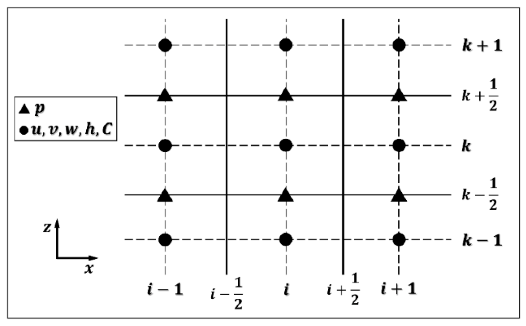
2.2. Numerical Methods

The above equations are discretized by a combined finite-volume and finite-difference scheme with a Godunov-type method for the spatial discretization and a two-stage (second-order) SSP Runge–Kutta (R-K) scheme [31] for time stepping. Compared with the standard R-K scheme, SSP R-K scheme has TVD properties and stronger nonlinear stability to deal with discontinuities in the solution [31]. Every R-K stage can be split into a hydrostatic predictor phase and the non-hydrostatic corrector phase. Here, we only illustrate the first stage of R-K scheme. In the hydrostatic predictor phase, an intermediate quantity U*, where U = (Du, Dv, Dw)^T, is calculated using momentum equations with the dynamic pressure term neglected,

$$\frac{{\mathit{U}}^{\ast }-{\mathit{U}}^n}{\mathrm{\Delta }t}=-\nabla \mathsf{\Theta }\left({\mathit{U}}^n\right)+{\mathit{S}}_h+{\mathit{S}}_{\rho }+{\mathit{S}}_{\tau },$$

(12)

where Uⁿ represents the U at time step n. In the non-hydrostatic phase, the velocity field is corrected by the dynamic pressure term:

$$\frac{{\mathit{U}}^{\left(1\right)}-{\mathit{U}}^{\ast }}{\mathrm{\Delta }t}={\mathit{S}}_p,$$

(13)

where the superscription (·)⁽¹⁾ represents the first stage for the R-K scheme. Substituting Equation (13) into the continuity equation, which is

$$\frac{\partial u}{\partial x}+\frac{\partial u}{\partial \sigma }\frac{\partial \sigma }{\partial x^{\ast }}+\frac{\partial v}{\partial y}+\frac{\partial v}{\partial \sigma }\frac{\partial \sigma }{\partial y^{\ast }}+\frac{1}{D}\frac{\partial w}{\partial \sigma }=0,$$

(14)

yields the Poisson equation of the dynamic pressure:

$$\begin{array}{l}\frac{\partial }{\partial x}\left(\frac{\partial p}{\partial x}+\frac{\partial p}{\partial \sigma }\frac{\partial \sigma }{\partial x^{\ast }}\right)+\frac{\partial }{\partial y}\left(\frac{\partial p}{\partial y}+\frac{\partial p}{\partial \sigma }\frac{\partial \sigma }{\partial y^{\ast }}\right)+\frac{\partial }{\partial \sigma }\left(\frac{\partial p}{\partial x}\right)\frac{\partial \sigma }{\partial x^{\ast }}\\ +\frac{\partial }{\partial \sigma }\left(\frac{\partial p}{\partial y}\right)\frac{\partial \sigma }{\partial y^{\ast }}+\left[{\left(\frac{\partial \sigma }{\partial x^{\ast }}\right)}^2+{\left(\frac{\partial \sigma }{\partial y^{\ast }}\right)}^2+\frac{1}{D^2}\right]\frac{\partial }{\partial \sigma }\left(\frac{\partial p}{\partial \sigma }\right)\\ =\frac{\rho }{\mathrm{\Delta }t}\left(\frac{\partial u^{\ast }}{\partial x}+\frac{\partial u^{\ast }}{\partial \sigma }\frac{\partial \sigma }{\partial x^{\ast }}+\frac{\partial v^{\ast }}{\partial y}+\frac{\partial v^{\ast }}{\partial \sigma }\frac{\partial \sigma }{\partial y^{\ast }}+\frac{1}{D}\frac{\partial w^{\ast }}{\partial \sigma }\right)\end{array}.$$

(15)

Equation (15) is discretized by the second-order central difference scheme and solved through iteration. The same procedure of above two phases is used for the second stage of the R-K scheme. The transport of a passive tracer is calculated using Equation (10) with the velocity field corrected in the non-hydrostatic phase. Besides, the time step is adaptive during the simulation and determined by the Courant–Friedrichs–Lewy (CFL) criterion with the Courant number. The Courant number was set to be 0.5 in this study.

In order to apply the Godunov-type method, all the variables are defined at the cell centers, except that dynamic pressure p is defined at the vertically-facing cell faces (Keller-Box scheme, Figure 2). For solving Equation (12), fluxes at cell faces are required. To reduce the numerical diffusion and simulating interfacial instability better, the HLLC approximate Riemann solver [32] is used to estimate the fluxes, which has widely been proved to be robust and efficient [27]. In this HLLC Riemann solver, the left and right velocities of U at cell face (i + 1/2) need to be calculated in a piecewise linear reconstruction method [33], which can be expressed as

$$\{\begin{array}{c}{\mathit{U}}_{i+\frac{1}{2}}^L={\mathit{U}}_i+\frac{1}{2}\left({\mathit{x}}_{i+\frac{1}{2}}-{\mathit{x}}_i\right)\mathrm{\cdot }\mathrm{\Delta }{\mathit{U}}_i\\ {\mathit{U}}_{i+\frac{1}{2}}^R={\mathit{U}}_{i+1}-\frac{1}{2}\left({\mathit{x}}_{i+1}-{\mathit{x}}_{i+\frac{1}{2}}\right)\mathrm{\cdot }\mathrm{\Delta }{\mathit{U}}_{i+1}\end{array},$$

(16)

where x represents the spatial coordinate value; ∆U_i represents the gradient of velocity at point x_i and needs to be reconstructed by slope limiters. The locations of variables in Equation (16) on the grid are illustrated in Figure 3.

In the advection and diffusion equations, the convective fluxes are determined using the hybrid linear/parabolic approximation (HLPA) scheme [34], which is a low-diffusive and oscillation-free convection scheme and has an approximately second-order accuracy in space.

The solution procedure is illustrated in Figure 4.

2.3. Slope Limiter

The slope limiter is the central part of the piecewise linear reconstruction, which limits the values range of the slope ∆U_i (see Figure 3) in order to control numerical oscillations. In this model, the slope limiter is defined as a two-variable function:

$$\mathrm{\Delta }{\mathit{U}}_i=Lim\left(\frac{{\mathit{U}}_i-{\mathit{U}}_{i-1}}{{\mathit{x}}_i-{\mathit{x}}_{i-1}},\frac{{\mathit{U}}_{i+1}-{\mathit{U}}_i}{{\mathit{x}}_{i+1}-{\mathit{x}}_i}\right),$$

(17)

where Lim represents the slope limiter. In this paper, the performances of minmod [15], van Leer [22], Monotonized Central (MC) [23], and superbee [35] limiters were compared by simulations. These above-mentioned limiters can be expressed as:

$$\mathrm{minmod} \mathrm{limiter}: Lim\left(a,b\right)=\min \mathrm{mod}\left(a,b\right),$$

(18)

$$\mathrm{van} \mathrm{Leer} \mathrm{limiter}: Lim\left(a,b\right)=\left(a\left|b\right|+\left|a\right|b\right)/\left(\left|a\right|+\left|b\right|\right),$$

(19)

$$\mathrm{MC} \mathrm{limiter}: Lim\left(a,b\right)=\mathrm{minmod}\left(2a,\left(a+b\right)/2,2b\right),$$

(20)

$$\mathrm{superbee} \mathrm{limiter}: Lim\left(a,b\right)=\mathrm{maxmod}\left(\mathrm{minmod}\left(2a,b\right),\mathrm{minmod}\left(a,2b\right)\right),$$

(21)

where the minmod function (maxmod function) is identically equal to zero if all of its arguments do not have the same sign, and otherwise it returns the argument with a minimal (maximal) absolute value.

In order to facilitate the analysis of the numerical characteristics of slope limiters, we rewrote the limiters as one-variate functions ϕ based on the on the ratio of the successive step. Assuming an equidistant computational mesh, we defined the successive steps R = (U_i+1 − U_i)/(U_i − U_i−1) = b/a. Then, by some algebraic transformations (details can be found in [36]), the slope limiters (18)~(21) were rewritten in an equivalent form ϕ(R).For all limiters, ϕ(R) = 0 when R ≤ 0; and for R > 0, the functions ϕ of the above-mentioned limiters can be written as:

$$\mathrm{minmod} \mathrm{limiter}: \varphi \left(R\right)=\min \left(\frac{2}{1+R},\frac{2R}{1+R}\right),$$

(22)

$$\mathrm{van} \mathrm{Leer} \mathrm{limiter}: \varphi \left(R\right)=\frac{4R}{{\left(1+R\right)}^2},$$

(23)

$$\mathrm{MC} \mathrm{limiter}: \varphi \left(R\right)=\min \left(1,\frac{4}{1+R},\frac{4R}{1+R}\right),$$

(24)

$$\mathrm{superbee} \mathrm{limiter}: \varphi \left(R\right)=\max \left[\min \left(\frac{4R}{1+R},\frac{2}{1+R}\right),\min \left(\frac{4}{1+R},\frac{2R}{1+R}\right)\right],$$

(25)

The graph of these limiters (22)~(25) are all plotted in Figure 5. The shaded region is the second-order TVD region, and choosing a limiter function within this region is necessary for second-order accuracy. The minmod and superbee limiter follow the lowest and highest boundary of the shaded region respectively; the van Leer and MC are both defined in the internal domain of the TVD region. As for ϕ(R) = 0, there is no dissipation; for ϕ(R) < 1, it means the limiter is dissipative; for ϕ(R) > 1, the limiter is anti-dissipative or compressive, which can steepen the gradient.

For a fixed R, the minmod limiter always takes the smallest slope value and the value is always less than 1, which means that it is the most dissipative limiter. While, the superbee limiter has a value over ϕ(R) = 1, so that it is the only one that has anti-dissipation here. As for MC limiter, it avoids the anti-dissipation compared with the superbee limiter. The van Leer limiter is the only one whose function is smooth when R > 0 among these four limiters involved.

3. Numerical Experiments

In this section, performances of the above-mentioned four slope limiters are examined in two case studies. The first case is the simulation of shear instability in the two-layer water environment, which aimed to verify the model’s capabilities of shear instability simulation and demonstrate the effects of different limiters. In this case, we mainly concentrated on the generation of K-H instability and the spatiotemporal features of mixing. The second case is the lock-exchange problem, which has been extensively used to study the dynamics and mixing mechanism of stratified flows. As a prototype problem, the lock-exchange flow, to some extent, can reflect the shear instability caused by gravity flow, which widely exists in natural fluids. For this case, we focused more on the model accuracy and the interfacial structures of vortices.

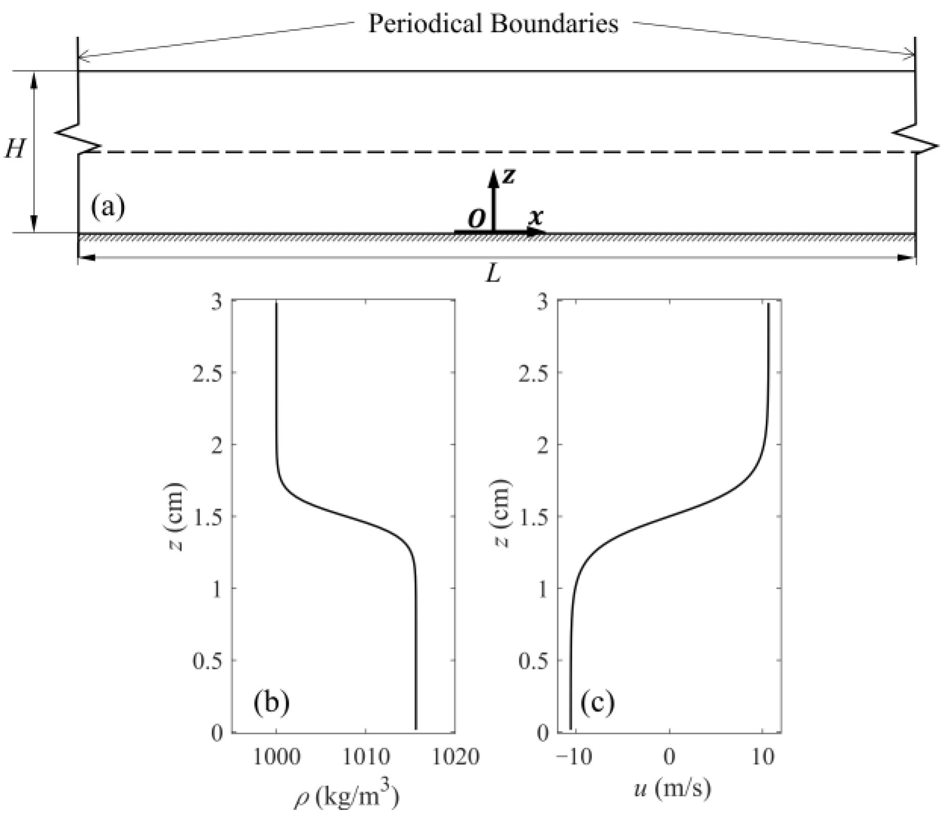
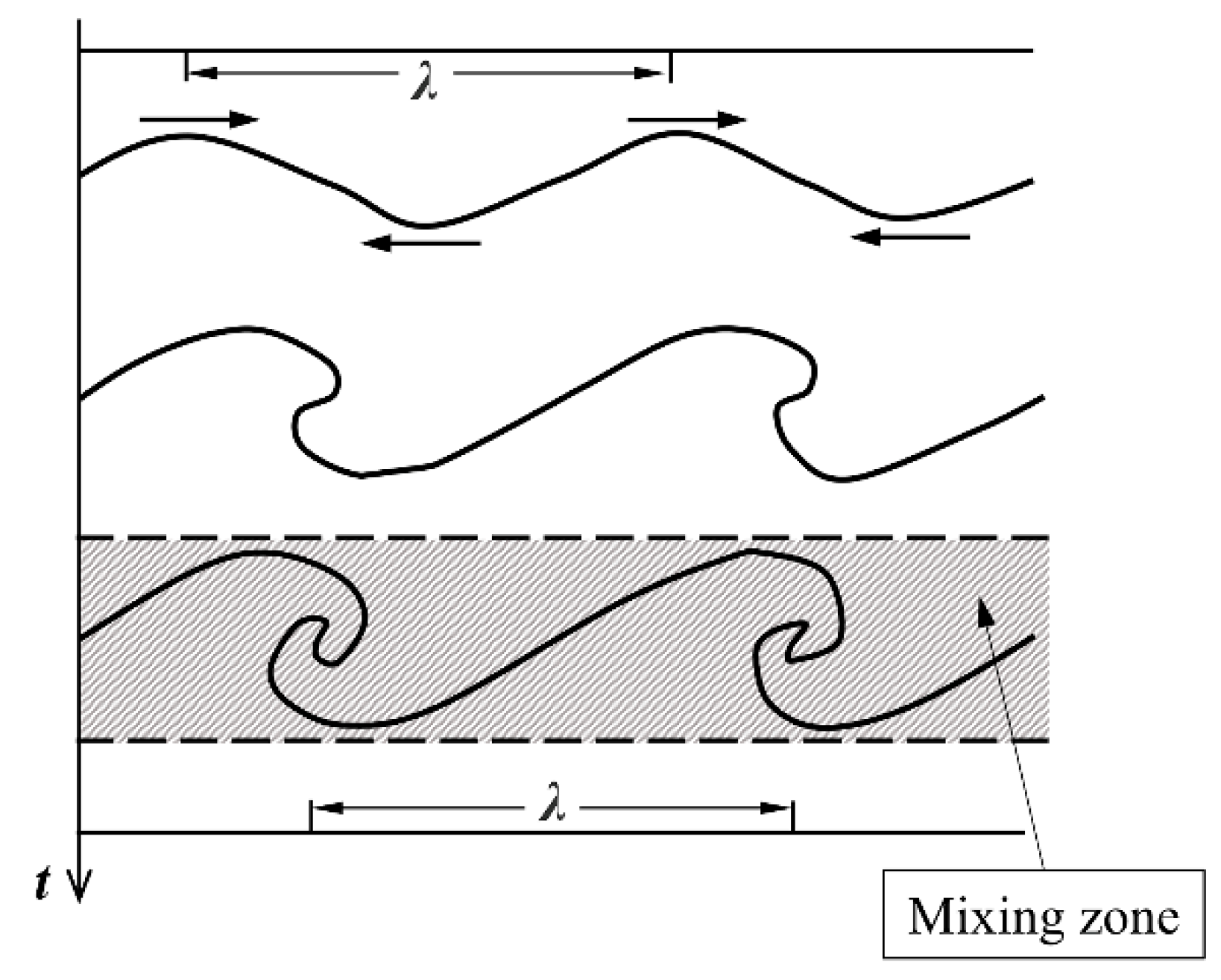
3.1. Shear Instability

To test the ability of the model to simulate the shear instability, we started with a simple test with the similar setups to the non-hydrostatic study by Bourgault and Kelley [19]. We established a two-dimension vertical numerical tank (See Figure 6a). The no-slip boundary condition was applied at the bottom, and periodic boundary conditions were imposed both at the left and right ends. In order to obtain enough interfacial K-H vortices in the computational domain and compare with the results of laboratory experiment by Thorpe [37], the length of the computational domain was set to L = 0.512 m, which is roughly equivalent to the measured area in Thorpe’s experiment [37]. In this test case, the total simulation time was 3.0 s, which is sufficient for the developments of interfacial billows. Considering the influence of the grid resolution on limiters’ performances, a set of different grid sizes (see

Table 1. A summary of grid settings in the shear instability case.

Case No.	Nx × Nz *	Δx (m)	Δσ
1	128 × 100	0.004	0.010
2	256 × 100	0.002	0.010	baseline case
3	512 × 100	0.001	0.010
4	256 × 50	0.002	0.020
5	256 × 200	0.002	0.005

* In this table, N_x and N_z represent the numbers of the grid in the x and z directions respectively.

) were applied in simulations. In the horizontal and vertical direction, the uniform grids were adopted respectively. Besides, the coefficients of viscosity were set to ν = 1.0 × 10⁶ m²/s in the simulations.

Initially, the water depth H = 0.03 m. The density is longitudinally uniform and its vertical distribution is defined as

$$\rho \left(x,z\right)={\rho }_1+\frac{\mathrm{\Delta }\rho }{2}\left[1+\tanh \left(\frac{z-z_i}{\mathrm{\Delta }\delta }\right)\right],$$

(26)

where ρ₁ = 1000.0 kg/m³ is the density of the upper layer, Δρ = 15.6 kg/m³ is the difference of density between lower and upper layer, ρ₂ = ρ₁ + Δρ is the density of the lower layer, Δδ = 0.15 cm is the density interface thickness and z_i = 0.5H. The initial vertical velocity was set to be zero. The initial horizontal velocity u was set to be longitudinally uniform and its vertical distribution is prescribed by the specifying Richardson number Ri, which is given by

$$Ri=\frac{g}{\rho }\frac{\partial \rho /\partial z}{{\left(\partial u/\partial z\right)}^2}.$$

(27)

According to the theory by Taylor-Goldstein Equation, the necessary condition of shear instability is Ri < 0.25 [38]. While, in some previous laboratory experiments [39] and numerical simulations [40,41], the K-H billows were observed if Ri fell below 0.1. For simulations in this test case, we used Ri = 0.025, which determines the vertical distribution of horizontal velocity (see Figure 6b,c).

To trigger the instability, a white noise of the amplitude 10⁻⁵ m/s was added into the horizontal velocity fields before simulating. For all cases with a fixed grid resolution, we applied the same white noise to velocity u. After a period of simulation time, some unstable waves appeared at the pycnocline layer, and then would develop to the rolled-up vortices, as shown in Figure 7. In terms of the spatial variation, the distance between consecutive local peaks or rolls is the significant feature, which is called the wavelength of the unstable wave. In most laboratory observations and numerical simulations, the wavelength is not usually constant. In this section, we measured the λ of the simulation results (see Figure 8).

For the simulation with a fixed grid size, the wavelength of unstable instability obtained by minmod limiter was largest, which means that the number of the K-H vortices captured by the minmod limiter was smallest. The superbee could capture the most numerous interfacial vortices here. The results with van Leer and MC limiters tended to be similar. Besides, the grid resolution, especially the horizontal resolution, had a noticeable influence on the generation of the instability. Refining the horizontal grids can decrease the wavelengths λ, so that the more small-scale K-H vortices can be captured. As for minmod limiter, the effects of grid resolution were most significant. Moreover, for van Leer and MC limiters, the results of λ were comparable to the laboratory observations of [37], except for the results with the coarsest mesh (N_x × N_z = 128 × 100). For the superbee limtier, the wavelengths would be slightly smaller than the observations with the continuous increase in horzontal grid number.

Apart from the differences in spatial domain, there were still temporal differences between the simulations with different slope limiters. Figure 9 presents the horizontal mean density ⟨ρ⟩ at t = 2.4 s, where $\langle \rho \rangle ={\displaystyle {\int }_{-L/2}^{L/2}\left(\rho -{\rho }_1\right)/\left({\rho }_2-{\rho }_1\right)}$. The ⟨ρ⟩ profiles in Figure 9 illustrates the progress of mixing, which also reveals the developments of the interfacial instability. After the appearance of noticeable vortices in the interface, a mixing zone is generated, and its thickness will expand as the K-H vortices grow (see Figure 7). As for the minmod limiter, the density layering was still notable at t = 2.4 s with any grid resolutions. While, at the same time, the superbee limiter made the mixing zone expand to around 2H/3 in the vertical length, which was larger than any results of the other limiters. These profiles illustrate that in the case of the superbee limiter, the K-H instability and vortices developed fastest, while the minmod limiter slowed down the developments significantly. The van Leer and MC limiters led to medium effects, and the effects by them could be notably influenced by grid resolutions. Horizontal resolution had a marked impact on the van Leer and MC limiters. In the coarse mesh, the effects of these two limiters were very similar to the minmod limiter (see Figure 9a); with the grid resolution increasing horizontally, the effects of the van Leer and MC limiters tended to get close to the effects of the superbee limiter (see Figure 9b,c). Using the finer vertical grids had no significant influence on the performance of the van Leer and MC limiters. Besides, in general, the results of employing the MC limiter showed a faster development rate of instability and mixing than that of the van Leer limiter.

In addition, we compared the simulation results with the laboratory observations by Thorpe [37]. We found that the results of the van Leer or MC limiters with N_x = 256 were comparable to the observations in terms of wavelength, growth rate, amplitude, and shape. Although, in the results of the superbee limiter with the resolution N_x × N_z = 128 × 100, the instability wavelengths observed were close to laboratory observations (Figure 8), the growth rate of K-H vortices were obviously higher than laboratory results. Figure 10 shows the comparison of developments of the unstable wave between simulation results of baseline cases (Figure 10a,b) and laboratory results (Figure 10c). Qualitatively, these simulations can reproduce the development of shear instabilities.

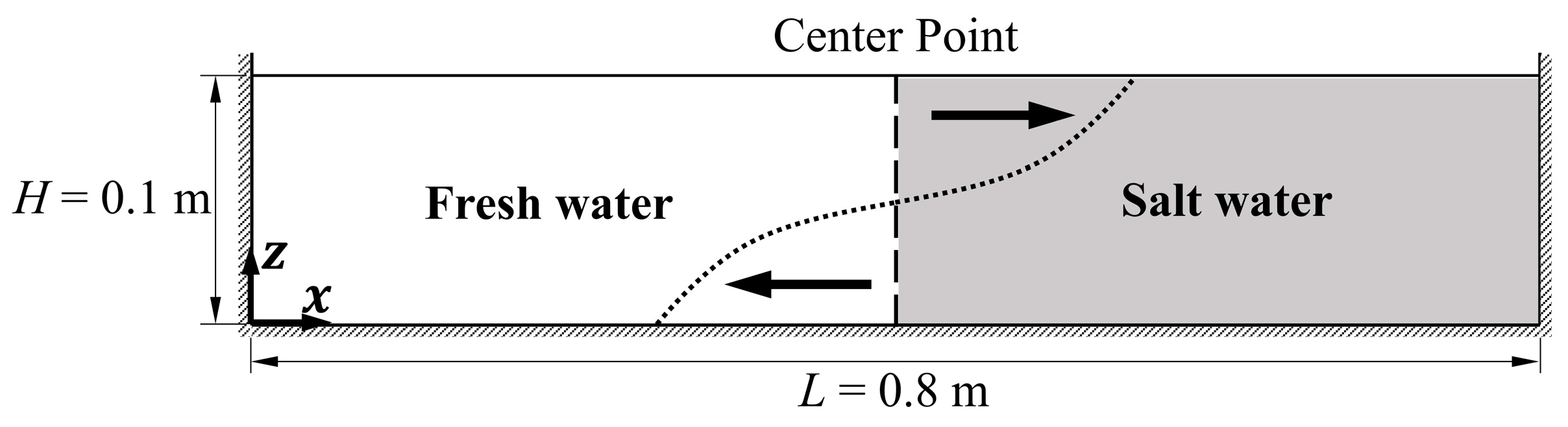
3.2. Lock-Exchange Problem

Lock-Exchange is the gravitational adjustment of two fluids of different density initially separated by a vertical gate [28], which involves some complex and typical physical phenomena, such as frontal movements and the mixing by interfacial instability. As a result, the lock-exchange problem is an important case that is of great significance for understanding the space-time features of stratified flows or gravity flows in natural fluids.

In this section, a full-depth lock-exchange flow simulation is conducted with the similar parameters of a direct numerical simulation (DNS) by Härtel et al. [42] and several non-hydrostatic studies [28,43,44]. The computation domain was a two-dimension vertical rectangular tank filled with two fluids of different density that were separated initially by a vertical gate at the center point. The tank had a length L = 0.8 m, and an initial water depth H = 0.1 m. In this study, the light fluid was set to be fresh water (zero salinity) and the heavy water was set to be salt water (Figure 11). At the initial moment, the salinity (S) distribution is defined as

$$S\left(x,z\right)=\{\begin{array}{cc}1.3592& x\ge 0.4m\\ 0& x<0.4m\end{array}.$$

(28)

The density ρ is assumed to be expressed as

$$\rho =999.972\times \left(1+0.75\times {10}^{-3}S\right).$$

(29)

Then, in this tank, the density of fresh water and salt water are ρ₁ = 999.972 kg/m³ and ρ₂ = 1000.991 kg/m³ respectively. Thereby, the reduced gravity g_0′ = g∆ρ⁄ρ₀ = 0.01 m/s², where ρ₀ is the reference density specified as 1000 kg/m³ and g is the gravitational acceleration constant with a value of 9.81 m/s².

In this test, the computational grids were uniform in the x- and z-direction, respectively. To examine the influence by grid resolution, a set of different grid sizes (see

Table 2. A summary of grid settings in the lock-exchange case.

Case No.	Nx × Nz *	Δx (m)	Δσ
1	200 × 100	0.004	0.010
2	400 × 100	0.002	0.010	baseline case
3	800 × 100	0.001	0.010
4	400 × 50	0.002	0.020
5	400 × 200	0.002	0.005

* In this table, N_x and N_z represent the numbers of the grid in the x and z direction, respectively.

) were used in simulations. In order to test the conservation and compare the results of this study with DNS results by Härtel et al. [42], the model ran on inviscid and constant viscous conditions respectively, and the model was integrated for 30 s.

After the center gate was removed at t = 0 s, the process of density current began with the initial state. The salt water flowed underneath the lighter fresh water and the velocities of two fluids were of opposite sign (see Figure 11). In general, with the increasing of the velocity shear, the K-H instability appeared, and a chain of well-defined billows could be seen along the interface of two fluids.

3.2.1. Inviscid Cases

Figure 12 compares the density fields at 15.0 s between the cases with different slope limiters and different grid resolutions in inviscid simulations. As we can see, no K-H instability could be observed in the simulations with the minmod limiter in any grid resolutions, which means that the interfacial mixing effects were omitted when minmod limiter was used. As for the superbee limiter, the model failed to capture the well-defined structures of the front and K-H billows, and a great number of non-physical small-scale vortices appeared at the interface. The results of van Leer and MC limiters were similar, and they could both capture the well-defined interfacial structures except in the simulations with excessively coarse mesh (N_x × N_z = 200 × 100). As for van Leer and MC limiters, the horizontal resolution had a more significant influence on simulating performance compared with vertical resolution.

Besides, for the results of the superbee limiter, the growing fluctuations of free surface could be detected, which is a sign of numerical oscillation. Figure 13 shows the free surface elevations of the simulations with the superbee limiter at t = 18.0 s, which indicates that the oscillation amplitude in the case with the N_x × N_z = 800 × 100 was several orders of magnitude greater than that in other cases. Additionally, the notable oscillation significantly influenced computational instability, which caused the model to not survive the long simulation.

In order to further investigate the limiters’ influence on model accuracy quantitatively, the energy conservation was tested. We define the total energy (TE) of the system:

$$\mathrm{TE}=\mathrm{PE}+\mathrm{KE}={\displaystyle {\int }_0^L{\displaystyle {\int }_0^H\rho gzdxdz}}+{\displaystyle {\int }_0^L{\displaystyle {\int }_0^H\frac{1}{2}\rho (u^2+w^2)dxdz}}.$$

(30)

where PE and KE are the potential and kinetic energies respectively. With no viscosity, the TE is supposed to remain unchanged. When t = 0, the initial KE₀ = 0 and the initial TE₀ can be calculated by Equation (30) as TE₀ = PE₀. If TE remains conservative, TE/TE₀ is always equal to 1.0, and we can estimate the energy conservation by the difference values between TE/TE₀ and 1.0 (i.e., |TE/TE₀ − 1.0|). Take the case of the resolution N_x × N_z = 400 × 100 for example; the time series of normalized dimensionless KE, PE, and KE are shown in the Figure 14. For the van Leer and MC limiters, the values of |TE/TE₀ − 1.0| were O (10⁻⁴) or less, which indicates that they just had minor influences on the accuracy in terms of energy conservation. In contrast, the minmod limiter introduced a notable error that led to the noticeable loss of the TE of the system. For the superbee limiter, the TE increased rapidly after around t = 10.0 s. Then, the superbee limiter caused calculating divergence, which influences computational stability.

For the simulations with the other grid sizes, we can also obtain results similar to Figure 14. In sum, van Leer and MC limiters both performed well in controlling dissipation and oscillation, while the minmod and superbee limiters were not feasible for simulation of this case because of the notable dissipation and overshooting respectively.

3.2.2. Constant Viscosity Cases

In order to compare with the DNS results of [42], we conducted the simulations with the same setup with the Grashof number $Gr=(\sqrt{g{\prime }_{0}H/2}H/(2\nu ){)}^2$=1.25 × 10⁶ (where ν is the molecular diffusivity that is specified as 10⁻⁶ m²/s) here. The front velocities and interfacial structures were investigated in this comparison, which are the key features of lock-exchange flows. To characterize the motion of intrusion front, a Froude number (Fr) was adopted where $Fr=u_f/\sqrt{{g^{\prime }}_{0}H/2}$ and u_f is the speed of the propagation of intrusion front in the stage of uniform motion.

Figure 15 depicts the density distributions for the simulations in this study and the DNS results by Härtel et al. [42] at t = 10T, where $T=\sqrt{H/2{g^{\prime }}_0}$. Similar to the results of inviscid simulations, the minmod limiter could not capture the interfacial instability, and the superbee limiter also failed to reproduce the well-defined K-H vortex structures and over-predicted the mixing. Most results of the minmod and superbee limiters illustrate that the front velocities were below the value of the DNS result. While, the front values of velocity obtained by the results with van Leer and MC limiters were very close to but slightly higher than the value of the DNS result. Considering the shapes of the intrusion fronts and structures interfacial vortices, only one case with the resolution N_x × N_z = 800 × 100 and MC limiter reproduced a comparable result to the DNS simulation, which depicted the heads intersecting with the bottom surfaces at an angle of around 60° and five noticeable and developed K-H vortices along the interface. Although the model with the van Leer limiter could reproduce the well-defined interfacial structures, the simulated results of the van Leer limiter did not demonstrate some key features, such as the K-H vortex in the center of the computational domain (see Figure 15b).

Different interfacial structures indicate distinct-different evolutions of the K-H instability and mixing features. Herein, we quantify the spatial features of mixing based on the height given by the following equations.

$$\begin{array}{cc}\overline{h\left(x,t\right)}=\frac{\overline{g^{\prime }h\left(x,t\right)}}{{g^{\prime }}_0},& \overline{g\prime h\left(x,t\right)}=g{\displaystyle {\int }_0^H\frac{\rho \left(x,z,t\right)-{\rho }_1}{{\rho }_2}}dz\end{array},$$

(31)

where $\overline{g^{\prime }h}$ represents the buoyancy effects. If the interface between two fluids was sharp and there had been no mixing, then $\overline{h\left(x,t\right)}$ would be the height of the interface at each horizontal location [45]. The mixing effects lead to reducing the local $\overline{h\left(x,t\right)}$ and smearing out the interface, so that $\overline{h\left(x,t\right)}$ will be noticeably smaller than the maximum height of the dense water mass (h_d). Taking the results with the resolution N_x × N_z = 800 × 100 as an example, $\overline{h}$ and the difference $\overline{h}-h_d$ at t = 10T are plotted in Figure 16, where h_d is defined as the maximum level of iso-density (ρ₁ + 0.02 ∆ρ). For the minmod limiter, $\overline{h}$ and h_d were almost equal, which means there was little mixing effect in the simulation. In the results of the van Leer and MC limiters, the relatively large difference $\overline{h}-h_d$ could be observed, which corresponds to the regions where the interfacial vortices developed. The superbee limiter predicted a mixing region in a wide range, but the flow structures were completely disordered and non-physical.

By the graphs of $\overline{h}-h_d$, the primary mixing regions of lock-exchange flow can be identified. In terms of mixing regions, the van Leer and MC limiters varied significantly in the simulation. The van Leer limiter tended to obtain a pair of the primary mixing regions behind the fronts, in contrast to the mixing region of the MC limiter close to the center. This difference can exert an influence on the simulation of the subsequent evolution of mixing, which can affect our understanding about stratified flows or gravity flows when we apply the hydrodynamic modelling in study.

4. Discussion

4.1. Numerical Dissipation

In general, the performances of slope limiters are associated with their different characteristics of numerical dissipation. In the present study, simulation results illustrated that the increasing dissipation of slope limiter could make the mixing process slow down (Figure 9) and even decrease the total energy of an inviscid system (Figure 13). In previous studies, similar effects by limiters have been recognized that were called the damping effects of numerical dissipation of limiters. For instance, in the research on surface wave modelling, the dissipation can decrease the wave amplitude (wave energy) and slow down the wave propagation [25]. It can be seen, for the cases of K-H instability and surface wave, that the damping effects of dissipation both influence the energy conservation and transformation.

While, more performances of the limiters’ dissipation can be found in K-H instability modellings, which has not been emphasized and fully discussed before. The increasing dissipation can reduce the numbers of simulated K-H vortices (Figure 8), and overmuch numerical dissipation, such as the dissipation introduced by minmod limiter, can even totally suppress the generation of K-H instability. Besides, by comparing the lock-exchange simulations with MC and superbee limiters (Figure 12 and Figure 15), we found anti-dissipation can make the model fail to control oscillation because the significant difference between MC and superbee limiters is that MC avoids the anti-dissipation that superbee has. Mathematically, the anti-dissipation can actually steepen the gradient [46]. The previous studies show that the process of steepening gradient can lead to staircasing of discontinuities in multi-dimensional cases [46], and even may not guarantee the non-oscillatory property of the TVD scheme [47]. Although there have been numerous robust implementations with the anti-dissipative limiters in hydrodynamic modelling (such as the shear instability case in this study), their practicability still needs attention and test verification.

From the perspective of numerical computation, the numerical dissipation can be produced during the discrete calculation of advection terms of momentum equation. In this study, the calculation of advection terms required the estimation of fluxes at cell faces, which are directly influenced by the slope limiter. It is regarded that the numerical dissipation can enhance or weaken the effects of diffusion term [48], which also explains the damping effects and numerical oscillations we found. On the one hand, increasing dissipation enhances the effects of diffusion term, so that it improves the model stability but can lead to excessive energy dissipation in simulations. On the other hand, the anti-dissipation of the superbee limiter weakened the effects of diffusion term, so the model stability could be influenced.

A further remark on the numerical dissipation is that the effects caused by different dissipations may not be demonstrated in terms of the noticeable introduced error or the influence on oscillation control. The van Leer and MC limiters were both medium-dissipation limiters, which can simulate the well-defined interfacial structures and did not introduce noticeable errors (Figure 14). However, the difference between these two limiters could lead to distinct differences on the evolution of K-H instability and mixing features in space (Figure 16), which can significantly affect our understanding about stratified flows or gravity flows when we apply the hydrodynamic modelling in research.

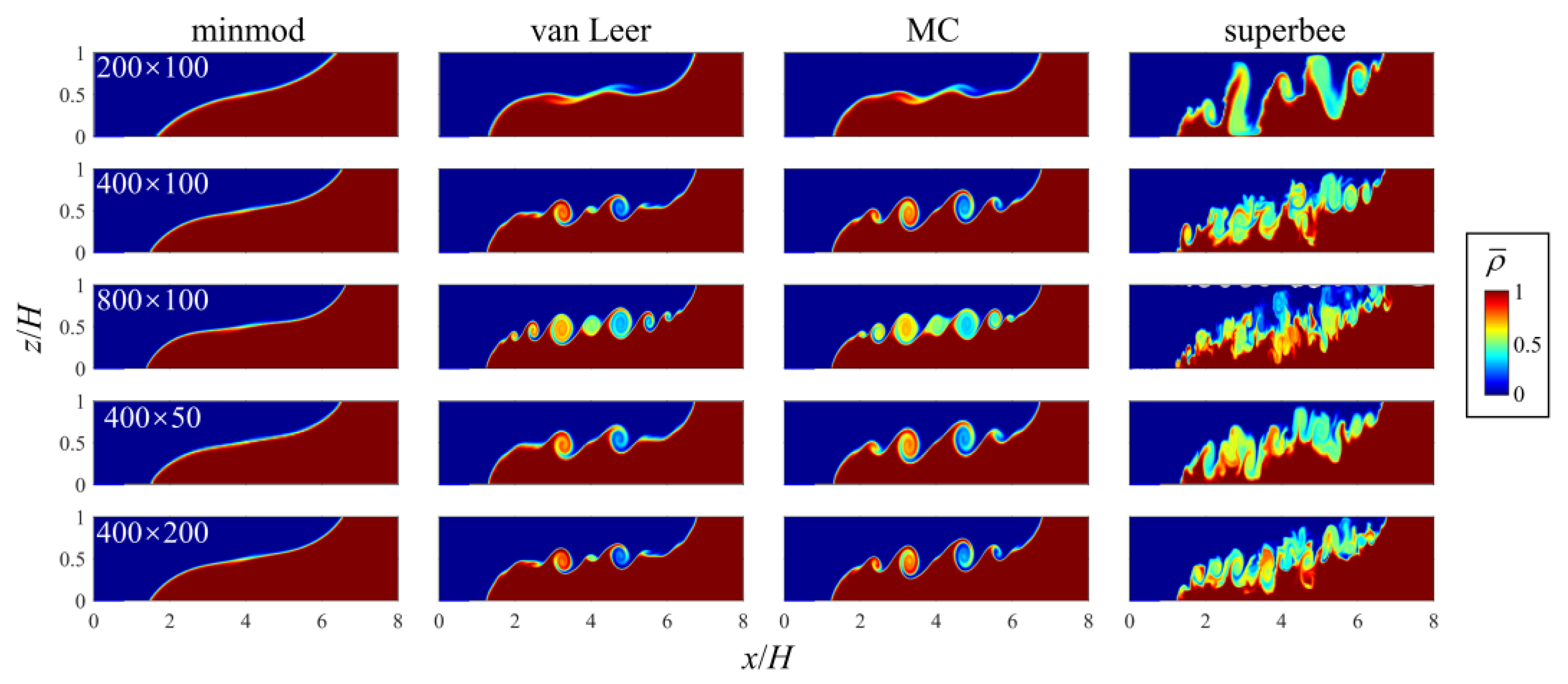
4.2. The Influence of Grid Resolution

From the perspective of the hydrodynamic model, grid resolution is an important influence factor of numerical dissipation, which attributes to the truncation errors in the discretized momentum equations [49]. In general, refiner grids can lead to less truncation errors so that the model with higher resolution experiences less numerical dissipation in simulation. For dissipative limiters (minmod, van Leer, and MC), refinement of girds weakens the damping effects of the slope limiter so that the development of interfacial instability (Figure 8, Figure 12 and Figure 15) and the process of mixing (Figure 9, Figure 12 and Figure 15) both become faster. In addition, less dissipation is helpful for the capture of refined dynamical structures. On the other hand, the decrease of dissipation of grid can make the anti-dissipation of limiter more prominent; as shown in the results of the lock-exchange cases with the superbee limiter (Figure 13), the finer grid can even bring more notable oscillations.

Furthermore, from a mathematical viewpoint, it also can be found from Equations (16) and (17) that there is a correlation between the limiters’ effects and the grid resolution. If refining the grid resolution, most the successive steps R in the field will move to the value of one, which makes the function values of four limiters closer. As shown in Figure 8 and Figure 9, the refinement of mesh can make the results with different limiters become more similar. Especially, for van Leer and MC limiters, these two limiters’ results in the coarse mesh were similar to minmod’s results, and they will be close to superbee’s results when refining the grids (Figure 9).

In this research, it also can be noticed that the influences of horizontal and vertical grid resolution were different in degree, and horizontal resolution had a more notable influence on the limiters’ performance. From a perspective of numerical dissipation, this difference may result from the horizontal flow playing a dominant role in flow fields of our test cases. For the K-H instability simulated in this study, the length scale in horizontal was larger than that in vertical, and the horizontal flow velocities were comparatively larger than vertical velocities on the whole. The dominant horizontal flows can result in the horizontal spatial truncation error dominating the vertical spatial truncation error [50]. In this regard, changing the horizontal resolution has a more notable influence on numerical dissipation so that it has a more significant impact on the limiters’ performance. Additionally, a similar feature of grid resolution can also be found in a stratified flows study based on the NHWAVE model [49]; they concluded that the vertical gird resolution has little influence on the numerical dissipation. Hence, the numerical dissipation and simulating performances were similar with different vertical grid resolutions, which is consistent with the results in this study. Although these results are only applicable to the present simulations, we expect very similar results from other stratified flow modellings because horizontal flow usually plays a leading role in natural stratified flows. Thus, our tests can provide information for other studies and possible issues in modellings of geophysical-scale flows.

Furthermore, it still needs attention that refining or coarsening the grids cannot help to eliminate the under- or over-prediction of mixing effects respectively. Although it is commonly agreed that refining the grid is helpful for improving simulation accuracy, the refinement of mesh may not help the model to reproduce a better result in some conditions, as shown in the results of lock-exchange simulations with the superbee limiter. Thus, compared to the grid resolution, the effects of the slope limiter should not be ignored even more. Apart from the method of refining mesh of all domain that we use, the Adaptive Mesh Refinement (AMR) seems to be a more efficient way to improve spatial accuracy. A recent study of hydrodynamic modelling [36] suggests that, in the framework of TVD method, the significance of limiter should not be ignored either for AMR scheme, because AMR actually leads to a stricter condition for slope limiting. While the influence of AMR on slope limiters was not studied here, it needs to be carried on in future research.

4.3. The Validity and Limitation of the Present Method of Slope Limiting

For the model applied in the present study, the slope limiters and the reconstruction method were developed based on the mathematical analysis of one-dimensional problems, which has many fundamental difficulties in multi-dimensional modelling. In some previous literature, the slope-limiting method applied in this study can be called ‘one-dimensional limiting’ [51,52]. Nonetheless, the one-dimensional limiting process has been widely applied in the great mass of hydrodynamic models so far [18,20,25]. The results represented in Section 3 showed that the model with some slope limiters (including van Leer and MC limiter) can reproduce the hydrodynamics processes that are comparable to laboratory observations or DNS results.

However, it is important to note that the noticeable introduced errors, staircasing of discontinuities, and computational instability also could be observed in the present simulations. An inappropriate method or slope limiter, such as the minmod and superbee limiters, may badly influence the accuracy, robustness, and convergence of numerical solutions for multi-dimensional modelling [51]. Some researchers noticed the effects of one-dimensional slope limiting in multi-dimensional hydrodynamic modelling [14,17,53], but few studies have discussed the problem in depth.

Additionally, as an alternative framework to extend the TVD slope-limiting method to multi-dimensional problems, the Multi-dimensional Limiting Process (MLP) has been devised and tested in several applications [51,54,55], especially in gas-dynamics modelling. However, some studies have shown that the MLP may decrease the simulation accuracy in continuous regions and in the case of steady problems [51]. Consequently, the MLP’s performance in the hydrodynamic modelling remains to be widely evaluated. Moreover, the slope limiter functions (18)~(21) are still applied in MLP methods, and this study can provide information for the studies of limiters’ effects in MLP methods.

5. Conclusions

An evaluating study on the effects of four slope limiters (minmod, van Leer, MC, and superbee) was conducted in the context of density stratified flows simulation. In this study, the numerical simulations based on a Godunov-type non-hydrostatic model, NHWAVE, were carried out to demonstrate the influences by different limiters on the predictions of shear instability and lock-exchange flow. The numerical results were carefully compared between one another and with the laboratory observations or DNS results.

Major conclusions of the present study can be drawn as follows:

• The performances of slope limiters were associated with their different dissipation characteristics. The dissipation can be regarded as ‘damping effects’ in simulation, which can suppress the generation of K-H instability and slow down the development of mixing. Anti-dissipation easily led to over-prediction of mixing and sometimes introduced numerical oscillation to trigger the calculating instability.
• Grid resolution can influence the limiters’ performances. Specifically, the horizontal resolution had a notable influence on simulations with different slope limiters in stratified shear flow simulations. Refining the grids can make the results of different limiters become more similar, but it may not work to reproduce a result in higher quality. Additionally, in application, an effective and suitable limiter ought to be prioritized over further refining the computational mesh.
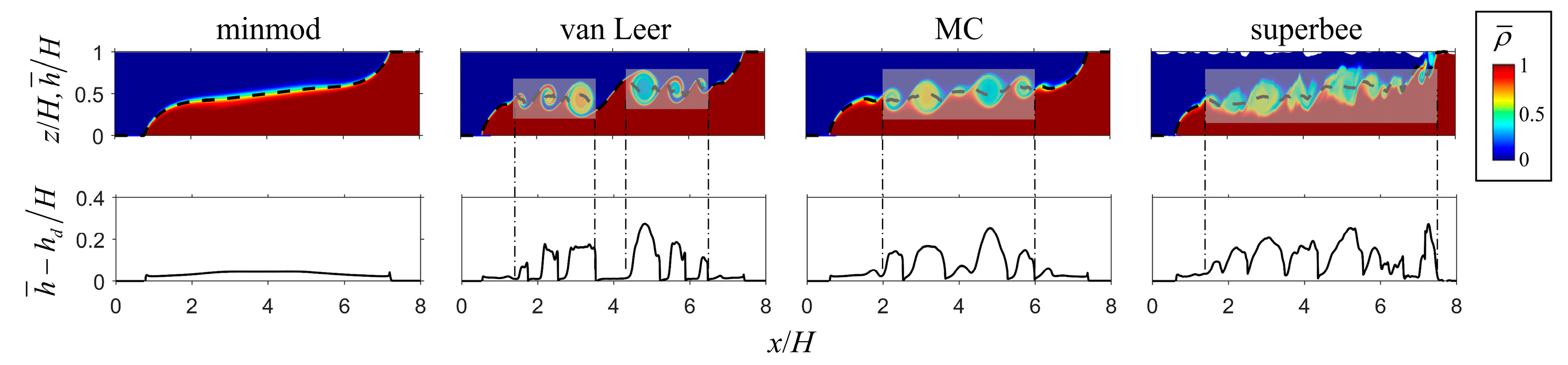
• In these two tests, the MC limiter had the best performance in simulating the well-defined structures of K-H vortex and did not introduce noticeable numerical errors in terms of energy conservation. Apart from that, the minmod limiter suppressed the generation of K-H instability and development of mixing noticeably because of its significant numerical dissipation; the superbee limiter could lead to non-physical vortices and over-predict mixing effects, and sometimes failed to control oscillation; the performance of the van Leer limiter was similar to that of the MC limiter, while in terms of the capture of interfacial structures, the MC limiter obtained a result that was much closer to DNS’s results in the case of the lock-exchange problem.
• Although the van Leer and MC limiters were similar on robust implementation and model accuracy, their different characteristics could lead to distinct-different simulated results in terms of the mixing features even in a very fine mesh. Their differences in the simulation can affect our understanding about the generation of shear instability and mixing and the hydrodynamical structures stratified flows.

The present results and analysis can provide information for choosing proper slope limiter and designing new slope-limiting methods in future hydrodynamic modelling. In addition, this study only provides the investigations on stratified shear flows on a laboratory scale and in relatively ideal conditions. A promising topic on large-scale and complex mixing processes deserves further study.

References

1. Geyer, W.R.; Lavery, A.; Scully, M.E.; Trowbridge, J.H. Mixing by shear instability at high Reynolds number. Geophys. Res. Lett. 2010, 37, L22607. [Google Scholar] [CrossRef] [Green Version]
2. Ivey, G.N.; Winters, K.B.; Koseff, J.R. Density Stratification, Turbulence, but How Much Mixing? Annu. Rev. Fluid Mech. 2008, 40, 169–184. [Google Scholar] [CrossRef]
3. Huang, H.; Imran, J.; Pirmez, C. Numerical Model of Turbidity Currents with a Deforming Bottom Boundary. J. Hydraul. Eng. 2005, 131, 283–293. [Google Scholar] [CrossRef]
4. Shi, J. Non-Hydrostatic Modelling of Vertical Mxing in Estuaries. Ph.D. Thesis, Hohai University, Nanjing, China, 2016. [Google Scholar]
5. Vlasenko, V.; Stashchuk, N.; McEwan, R. High-resolution modelling of a large-scale river plume. Ocean Dyn. 2013, 63, 1307–1320. [Google Scholar] [CrossRef]
6. Shi, J.; Tong, C.; Zheng, J.; Zhang, C.; Gao, X. Kelvin-Helmholtz Billows Induced by Shear Instability along the North Passage of the Yangtze River Estuary, China. J. Mar. Sci. Eng. 2019, 7, 92. [Google Scholar] [CrossRef] [Green Version]
7. Özgökmen, T.M.; Johns, W.E.; Peters, H.; Matt, S. Turbulent Mixing in the Red Sea Outflow Plume from a High-Resolution Nonhydrostatic Model. J. Phys. Oceanogr. 2003, 33, 1846–1869. [Google Scholar] [CrossRef] [Green Version]
8. Zhou, Z.; Yu, X.; Hsu, T.; Shi, F.; Geyer, W.R.; Kirby, J.T. On nonhydrostatic coastal model simulations of shear instabilities in a stratified shear flow at high R eynolds number. J. Geophys. Res. Oceans 2017, 122, 3081–3105. [Google Scholar] [CrossRef]
9. Özgökmen, T.M.; Fischer, P.F.; Duan, J.; Iliescu, T. Three-Dimensional Turbulent Bottom Density Currents from a High-Order Nonhydrostatic Spectral Element Model. J. Phys. Oceanogr. 2004, 34, 2006–2026. [Google Scholar] [CrossRef]
10. Özgökmen, T.M.; Fischer, P.F.; Duan, J.; Iliescu, T. Entrainment in bottom gravity currents over complex topography from three-dimensional nonhydrostatic simulations. Geophys. Res. Lett. 2004, 31, L13212. [Google Scholar] [CrossRef] [Green Version]
11. Shi, F.; Chickadel, C.C.; Hsu, T.-J.; Kirby, J.T.; Farquharson, G.; Ma, G. High-Resolution Non-Hydrostatic Modeling of Frontal Features in the Mouth of the Columbia River. Estuaries Coasts 2016, 40, 296–309. [Google Scholar] [CrossRef]
12. Stashchuk, N.; Vlasenko, V. Generation of internal waves by a supercritical stratified plume. J. Geophys. Res. Earth Surf. 2009, 114, C01004. [Google Scholar] [CrossRef] [Green Version]
13. Vlasenko, V.; Stashchuk, N.; Inall, M.E.; Hopkins, J.E. Tidal energy conversion in a global hot spot: On the 3-D dynamics of baroclinic tides at the Celtic Sea shelf break. J. Geophys. Res. Oceans 2014, 119, 3249–3265. [Google Scholar] [CrossRef] [Green Version]
14. Cao, X.; Zheng, J.; Shi, J.; Zhang, C.; Zhang, J. Evaluating the influence of slope limiters on nearshore wave simulation in a non-hydrostatic model. Appl. Ocean Res. 2021, 112, 102683. [Google Scholar] [CrossRef]
15. LeVeque, R.J. Finite Volume Methods for Hyperbolic Problems; Cambridge University Press: Cambridge, UK, 2002; Volume 31. [Google Scholar]
16. Erduran, K.S.; Kutija, V.; Hewett, C.J.M. Performance of finite volume solutions to the shallow water equations with shock-capturing schemes. Int. J. Numer. Methods Fluids 2002, 40, 1237–1273. [Google Scholar] [CrossRef]
17. Bai, F.-P.; Yang, Z.-H.; Zhou, W.-G. Study of total variation diminishing (TVD) slope limiters in dam-break flow simulation. Water Sci. Eng. 2018, 11, 68–74. [Google Scholar] [CrossRef]
18. Ma, G.; Shi, F.; Kirby, J.T. Shock-capturing non-hydrostatic model for fully dispersive surface wave processes. Ocean Model. 2012, 43–44, 22–35. [Google Scholar] [CrossRef]
19. Bourgault, D.; Kelley, D.E. A Laterally Averaged Nonhydrostatic Ocean Model. J. Atmospheric Ocean. Technol. 2004, 21, 1910–1924. [Google Scholar] [CrossRef] [Green Version]
20. González-Avilés, J.J.; Cruz-Osorio, A.; Lora-Clavijo, F.D.; Guzmán, F.S. Newtonian cafe: A new ideal MHD code to study the solar atmosphere. Mon. Not. R. Astron. Soc. 2015, 454, 1871–1885. [Google Scholar] [CrossRef] [Green Version]
21. Van Leer, B. Towards the ultimate conservative difference scheme. V. A second-order sequel to Godunov′s method. J. Comput. Phys. 1979, 32, 101–136. [Google Scholar] [CrossRef]
22. van Leer, B. Towards the ultimate conservative difference scheme. II. Monotonicity and conservation combined in a second-order scheme. J. Comput. Phys. 1974, 14, 361–370. [Google Scholar] [CrossRef]
23. Van Leer, B. Towards the ultimate conservative difference scheme. IV. A new approach to numerical convection. J. Comput. Phys. 1977, 23, 276–299. [Google Scholar] [CrossRef]
24. Sweby, P.K. High Resolution Schemes Using Flux Limiters for Hyperbolic Conservation Laws. SIAM J. Numer. Anal. 1984, 21, 995–1011. [Google Scholar] [CrossRef]
25. Choi, Y.-K.; Shi, F.; Malej, M.; Smith, J.M. Performance of various shock-capturing-type reconstruction schemes in the Boussinesq wave model, FUNWAVE-TVD. Ocean Model. 2018, 131, 86–100. [Google Scholar] [CrossRef]
26. Kirby, J.T. Boussinesq Models and Their Application to Coastal Processes across a Wide Range of Scales. J. Waterw. Port Coastal Ocean Eng. 2016, 142, 03116005. [Google Scholar] [CrossRef]
27. Ma, G.; Kirby, J.T.; Shi, F. Numerical simulation of tsunami waves generated by deformable submarine landslides. Ocean Model. 2013, 69, 146–165. [Google Scholar] [CrossRef]
28. Shi, J.; Shi, F.; Kirby, J.T.; Ma, G.; Wu, G.; Tong, C.; Zheng, J. Pressure Decimation and Interpolation (PDI) method for a baroclinic non-hydrostatic model. Ocean Model. 2015, 96, 265–279. [Google Scholar] [CrossRef] [Green Version]
29. Derakhti, M.; Kirby, J.T.; Shi, F.; Ma, G. NHWAVE: Model Revisions and Tests of Wave Breaking in Shallow and Deep Water; University of Delaware: Newark, DE, USA, 2015. [Google Scholar]
30. Phillips, N.A. A Coordinate System having Some Special Advantages for Numerical Forecasting. J. Meteorol. 1957, 14, 184–185. [Google Scholar] [CrossRef] [Green Version]
31. Gottlieb, S.; Shu, C.-W.; Tadmor, E. Strong Stability-Preserving High-Order Time Discretization Methods. SIAM Rev. 2001, 43, 89–112. [Google Scholar] [CrossRef]
32. Toro, E.F.; Spruce, M.; Speares, W. Restoration of the contact surface in the HLL-Riemann solver. Shock Waves 1994, 4, 25–34. [Google Scholar] [CrossRef]
33. Zhou, J.; Causon, D.; Mingham, C.; Ingram, D. The Surface Gradient Method for the Treatment of Source Terms in the Shallow-Water Equations. J. Comput. Phys. 2001, 168, 1–25. [Google Scholar] [CrossRef]
34. Zhu, J. A low-diffusive and oscillation-free convection scheme. Commun. Appl. Numer. Methods 1991, 7, 225–232. [Google Scholar] [CrossRef]
35. Roe, P.L. Some Contributions to the Modeling of Discontinuous Flows. Lect. Appl. Math. 1985, 22, 163–193. [Google Scholar]
36. Velechovsky, J.; Francois, M.; Masser, T. Direction-aware slope limiter for three-dimensional cubic grids with adaptive mesh refinement. Comput. Math. Appl. 2019, 78, 670–687. [Google Scholar] [CrossRef]
37. Thorpe, S.A. A method of producing a shear flow in a stratified fluid. J. Fluid Mech. 1968, 32, 693–704. [Google Scholar] [CrossRef]
38. Miles, J.W. On the stability of heterogeneous shear flows. J. Fluid Mech. 1961, 10, 496–508. [Google Scholar] [CrossRef] [Green Version]
39. Fructus, D.; Carr, M.; Grue, J.; Jensen, A.; Davies, P.A. Shear-induced breaking of large internal solitary waves. J. Fluid Mech. 2009, 620, 1–29. [Google Scholar] [CrossRef] [Green Version]
40. Barad, M.F.; Fringer, O.B. Simulations of shear instabilities in interfacial gravity waves. J. Fluid Mech. 2010, 644, 61–95. [Google Scholar] [CrossRef] [Green Version]
41. Lamb, K.G.; Farmer, D. Instabilities in an Internal Solitary-like Wave on the Oregon Shelf. J. Phys. Oceanogr. 2011, 41, 67–87. [Google Scholar] [CrossRef]
42. Härtel, C.; Meiburg, E.; Necker, F. Analysis and direct numerical simulation of the flow at a gravity-current head. Part 1. Flow topology and front speed for slip and no-slip boundaries. J. Fluid Mech. 2000, 418, 189–212. [Google Scholar] [CrossRef] [Green Version]
43. Fringer, O.; Gerritsen, M.; Street, R. An unstructured-grid, finite-volume, nonhydrostatic, parallel coastal ocean simulator. Ocean Model. 2006, 14, 139–173. [Google Scholar] [CrossRef]
44. Lai, Z.; Chen, C.; Cowles, G.W.; Beardsley, R.C. A nonhydrostatic version of FVCOM: 1. Validation experiments. J. Geophys. Res. Earth Surf. 2010, 115, C11010. [Google Scholar] [CrossRef] [Green Version]
45. Shin, J.O.; Dalziel, S.B.; Linden, P.F. Gravity currents produced by lock exchange. J. Fluid Mech. 2004, 521, 1–34. [Google Scholar] [CrossRef] [Green Version]
46. Berger, M.; Aftosmis, M.; Muman, S. Analysis of Slope Limiters on Irregular Grids; American Institute of Aeronautics and Astronautics: Reno, NV, USA, 2005. [Google Scholar] [CrossRef] [Green Version]
47. Lin, L.; Liu, Z. TVDal: Total variation diminishing scheme with alternating limiters to balance numerical compression and diffusion. Ocean Model. 2019, 134, 42–50. [Google Scholar] [CrossRef]
48. Patankar, S.V. Numerical Heat Transfer and Fluid Flow, 1st ed.; CRC Press: Boca Raton, FL, USA, 1980; ISBN 9781315275130. [Google Scholar]
49. Shi, J.; Shi, F.; Zheng, J.; Zhang, C.; Malej, M.; Wu, G. Interplay between grid resolution and pressure decimation in non-hydrostatic modeling of internal waves. Ocean Eng. 2019, 186, 106110. [Google Scholar] [CrossRef]
50. Wadzuk, B.M.; Hodges, B.R. Hydrostatic versus Nonhydrostatic Euler-Equation Modeling of Nonlinear Internal Waves. J. Eng. Mech. 2009, 135, 1069–1080. [Google Scholar] [CrossRef]
51. Kim, K.H.; Kim, C. Accurate, efficient and monotonic numerical methods for multi-dimensional compressible flows: Part II: Multi-dimensional limiting process. J. Comput. Phys. 2005, 208, 570–615. [Google Scholar] [CrossRef]
52. Yoon, S.-H.; Kim, C.; Kim, K.-H. Multi-dimensional limiting process for three-dimensional flow physics analyses. J. Comput. Phys. 2008, 227, 6001–6043. [Google Scholar] [CrossRef]
53. An, H.; Yu, S. An accurate multidimensional limiter on quadtree grids for shallow water flow simulation. J. Hydraul. Res. 2014, 52, 565–574. [Google Scholar] [CrossRef]
54. Kang, H.-M.; Kim, K.H.; Lee, D.-H. A new approach of a limiting process for multi-dimensional flows. J. Comput. Phys. 2010, 229, 7102–7128. [Google Scholar] [CrossRef]
55. Zhang, S.-T.; Chen, F.; Liu, H. Assessment of Limiting Processes of Numerical Schemes on Hypersonic Aeroheating Predictions. J. Thermophys. Heat Transf. 2016, 30, 754–769. [Google Scholar] [CrossRef]
Figure 1. (a) Schematic of stratified shear flows in the density stratification water; there are many small-scale structures of K-H instability at the interface. (b) Schematic of K-H vortices (by Geyer et al. [1]).
Jmse 10 00489 g001
Figure 2. Keller-Box layout of computational variables. Velocities (u, v, w), water depth (h), and passive tracer scaler (C) are all placed at cell center and dynamic pressure (p) is placed at vertical cell face.
Jmse 10 00489 g002
Figure 3. Schematic sketch of the locations of variables in Equation (16).
Jmse 10 00489 g003
Figure 4. Flow chart of the solution procedure of the NHWAVE model.
Jmse 10 00489 g004
Figure 5. Diagram of slope limiters in this study. The shaded region represents the second-order TVD region.
Jmse 10 00489 g005
Figure 6. (a) Schematic of the domain and the boundary condition, (b) initial density profile, and (c) horizontal velocity profile for the shear instability case.
Jmse 10 00489 g006
Figure 7. Schematic of the evolution of a K-H vortex at the interface.
Jmse 10 00489 g007
Figure 8. The wavelengths λ of the unstable wave obtained by simulation results. The shade zone represents the range of the wavelength data from the laboratory observation [37].
Jmse 10 00489 g008
Figure 9. Comparison of horizontal mean density profiles for the shear instability problem with the different slope limiters and different grid resolutions (left to right) at t = 2.4 s. The grid resolutions (Nx × Nz) of the subfigures (ae) are labeled at the top of these subfigures, respectively.
Jmse 10 00489 g009
Figure 10. Three sequences of snapshots taken at half-second intervals showing the growth of instability, obtained by simulation results with (a) van Leer and (b) MC limiters in the grid resolution Nx × Nz = 256 × 100 and the (c) laboratory observations of [37]. Subfigure (a,b) show the results of density distribution ( ρ ¯ = ρ ρ 1 / ρ 2 ρ 1 ).
Jmse 10 00489 g010
Figure 11. Schematic of lock-exchange domain and the initial condition of simulation. The arrows present the directions of the currents; the black dashed line indicates the gate between light and heavy fluid; the dotted line shows a diagrammatic view of the interface between the two fluids after the release.
Jmse 10 00489 g011
Figure 12. Comparison of density ( ρ ¯ = ρ ρ 1 / ρ 2 ρ 1 ) distributions for inviscid lock-exchange flows at t = 15.0 s with the different grid resolutions (top to bottom) and different slope limiters (left to right).
Jmse 10 00489 g012
Figure 13. The elevations η of surface at t = 18.0 s for the simulations of lock-exchange problem with the superbee limiter.
Jmse 10 00489 g013
Figure 14. Time series of TE/TE0, PE, and KE for the inviscid case of the lock-exchange problem with the grid resolution Nx × Nz = 400 × 100.
Jmse 10 00489 g014
Figure 15. (a) Comparison of the simulated density ( ρ ¯ = ρ ρ 1 / ρ 2 ρ 1 ) distributions for constant viscosity lock-exchange flow simulations with different slope limiters (left to right) and different grid resolutions (top to bottom) at t = 10T; (b) the simulated results by Härtel et al. [42]. The Fr represents the Froude number in that case.
Jmse 10 00489 g015
Figure 16. The horizontal distribution of h ¯ / H (the dashed lines in upper panels) and the difference ( h ¯ h d ) / H (lower panels) at t = 10T for the constant-viscosity cases of the lock-exchange problem with the grid resolution Nx × Nz = 800 × 100. The background images in the upper panels are the density distributions. The shaded areas represent the mixing regions.
Jmse 10 00489 g016