PDE Formation and Iterative Docking Control of USVs for the Straight-Line-Shaped Mission

Abstract

In this paper, an intelligent control scheme of formation collision avoidance and iterative docking is proposed for full-actuated unmanned surface vehicles (USVs). The artificial potential field method is integrated into the partial differential equation (PDE) formation control approach, which can improve the collision-avoidance performance of the formation. During the docking process of the straight-line formation, the USV agent is expected to track the desired commands accurately. Considering the possibility of docking failure, an iterative learning model predictive control (ILMPC) scheme is introduced. Once the moving USV fails in docking on the stationary USV, the moving agent can return to the origin to re-execute the docking process. The ILMPC method has the advantages of model predictive control and the iterative learning, so it can consider the future process dynamics in the time domain and overcome periodic disturbances. Simulation results show that USVs can avoid collisions with each other in the straight-line-formation mission. Furthermore, the USV agent can dock one-by-one successfully when interference exists.

1. Introduction

In recent years, with the development of intelligent technology and the growth of market demand, USV, as an intelligent mobile platform for navigating on water, lake, and sea surfaces, has been increasingly used in different fields such as military patrols, environmental monitoring, and maritime search and rescue [1]. As a result, the functions of transportation, recycling, and power supply are also expected to appear in USVs. In addition, USVs can also form one straight-line unit through connection between individuals to build a dynamic floating infrastructure [2]. In order to realize the successful docking of multi-USVs, a reliable docking method should be investigated.

The straight-line-formation mission of multiple USVs can be mainly divided into two parts: formation control and the docking of USVs. There have been numerous literature studies on the cooperative control of robots. Among them, research methods such as graph theory, topology, and matrices have made great advances in the formation control of multi-agents [3,4,5,6,7,8]. In recent years, the PDE has been proposed to address the formation control problem, which is inspired by viewing the distributed agent system as the discrete approximation of a PDE [9]. QI Jie et al. proposed a method of PDE that enables agents to track and maintain the desired formation via using low-cost agents with limited sensing range and limited computing power [10]. Hao Chen et al. proposed a distributed formation control method for ground mobile robots based on partial differential equations of reaction–convection–diffusion partial differential equations [11]. Furthermore, Thomas Meurer proposed the nonlinear PDE–based motion planning approach for the formation control of mobile agents [12]. Gerhard Freudenthaler designed a PDE-based multi-agent formation control strategy based on the planarity and backstepping techniques [13]. However, the size of the agent is mostly not considered in the PDE formation control algorithm, which may lead to the problem of agents colliding with each other during the formation movement. Thus, the PDE formation control approach should be enhanced in future studies.

During the docking process of USV, Morten Breivik et al. proposed a safe docking method for small USVs and large ships at sea [14]. The mother ship passively moves forward in a straight line, while the USV uses constant azimuth guidance to actively track the target point. The whole process is divided into two stages. In the first stage, the small USV moves to the target point of the mother ship’s safe positioning zone. In the second stage, the distance between the USV and the docking point is reduced until the position and speed of the USV meets the docking requirements of the target point. Wenyong Yu et al. proposed a tracking control algorithm based on the line-of-sight observation method to guarantee the command tracking quality [15]. Because a monocular vision system that can recognize the light source is installed on the USV, the docking target position can be obtained accurately. The USV is designed to near the mother ship gradually, and finally it can enter the stern ramp to complete the recovery. In addition to USVs, Tianqi Xie et al. employed the line-of-sight guidance law that provides outputs for the under-actuated underwater vehicle, so it can assist the vehicle in docking at the desired position efficiently [16].

Similar to the docking of USVs, the autonomous berthing of USVs also adjusts the position and attitude of the hull when arriving at the target point. Yulei Liao et al. introduced an improved adaptive fuzzy PID control approach to improve the USV trajectory-tracking performance [17]. Andreas B. Martinsen et al. proposed a method to realize the autonomous docking of ships utilizing the numerical optimal control strategy [18].

Whether it is the docking or the parking of USVs, the target point can be reached by tracking the setting trajectory precisely. There are several methods of trajectory tracking that work well. Tao Jiang et al. introduced an adaptive sliding mode control method based on the generalized predictive control (GPC) algorithm [19]. Zaopeng Dong et al. presented a backstepping control algorithm based on state feedback to solve the trajectory-tracking problem of under-actuated USVs on the horizontal plane [20]. Yixin Su et al. put forward an improved adaptive integral line-of-sight guidance law to track the planned path for USVs with uncertainties [21].

However, one of the main disadvantages of the above work is that the input or state constraints are not explicitly considered, which may lead to poor control performance and even damage to the actuator during implementation. Model predictive control (MPC) is a potential method to overcome these shortcomings because it employs the optimal control architechture [22]. MPC has obtained extensive attention in the field of trajectory control. Aiming at the position- and velocity-tracking problems of underactuated USVs, Mohamed Abdelaal et al. proposed the nonlinear model predictive control (NMPC) to address the collision avoidance of static and dynamic targets via introducing the sideslip angle compensation term and decreasing the environmental interference effects [23]. Ali Haseltalab et al. put forward a ship-trajectory-tracking MPC approach that considers the thrust distribution of the rotating propellers [24]. Aiming at the two-dimensional trajectory-tracking problem of autonomous surface vehicles, Huarong Zheng et al. presented NMPC and MPC linearization approaches, and proved their effectiveness [25]. Mohamed Abdelaal et al. used the NMPC to improve the collision-avoidance performance via adjusting the under-actuated elliptical surface ship position and speed [26].

Although MPC has a good control effect on the trajectory tracking of USVs, it is highly dependent on the dynamic model of the vessel. If the model is less accurate, it will have a great impact on the trajectory tracking of the USVs. Iterative learning control (ILC) can deal with the uncertainty of the actual system model as it is data-driven. In comparison, it requires less prior knowledge of the system and does not rely on a very accurate system model. It can be used to handle complex control problems such as the unknown parameters and model uncertainty. According to the dynamic characteristics of USVs, Yang Yang et al. proposed an adaptive iterative learning algorithm to optimize parameters [27]. In view of the model uncertainty and the external disturbance in the path-tracking process of USVs, Changkui Xu et al. presented an iterative learning observer to estimate the system state in the output feedback control design [28]. Lu Liu et al. proposed an adaptive controller design method for combining the dynamic surface controller design technique with iterative learning method, which can enable ships in formation to reach a reference position under the continuous disturbance of wind, waves and ocean currents [29].

On the basis of the above references, this paper investigates the iterative docking control of USV under the straight line formation task. The main work includes:

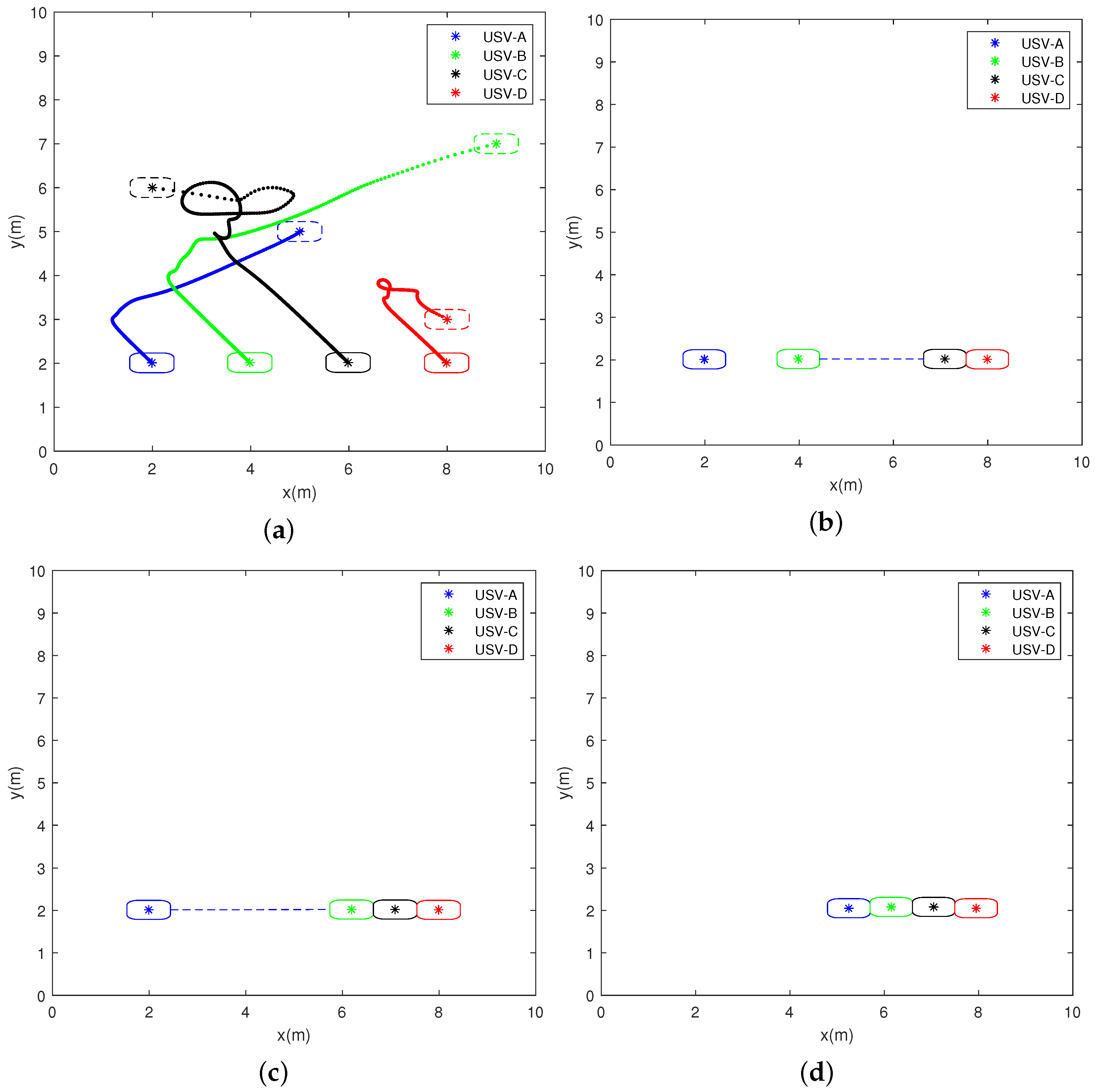
• In order to complete the formation task of USVs, this paper introduces the PDE as the control algorithm of the formation, and it uses the artificial potential field method to improve the effect of collision during the formation process.
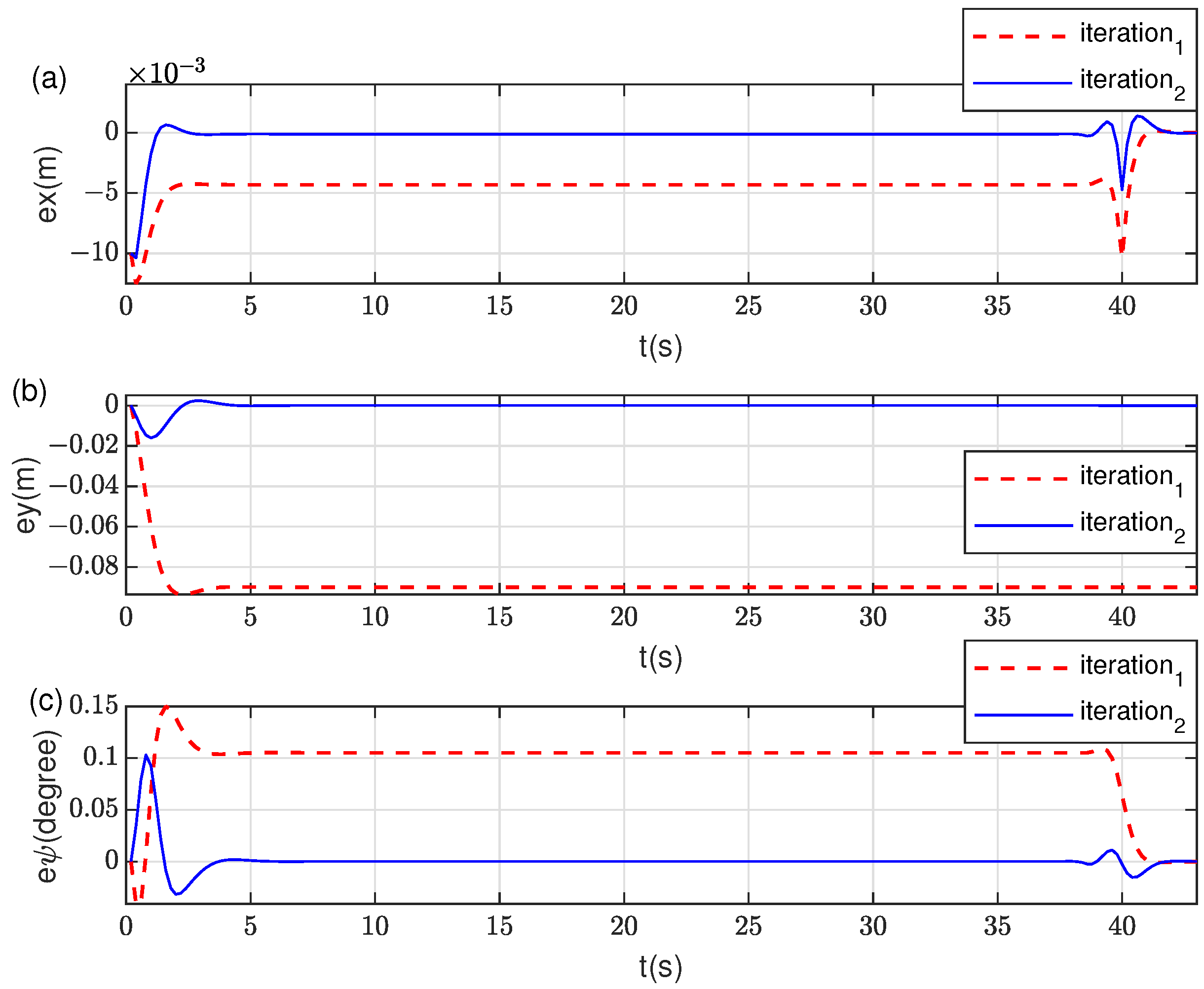
• Aiming at the requirement that USVs can go back to the original location and repeat the docking once the first docking fails, an ILMPC method is proposed that combines the advantages of iterative learning and model prediction control. Repetitive errors can be exploited by iterative learning to obtain precise results, while MPC can overcome environment disturbances via considering the future process costs.

The rest of the paper is organized as follows. Section 2 introduces the dynamics model of USV. In Section 3, an artificial potential field collision-avoidance algorithm based on PDE is proposed. Section 4 presents the ILMPC control algorithm. In Section 5, numerical simulation tests are carried out according to the proposed method. Section 6 summarizes the full paper.

2. Model

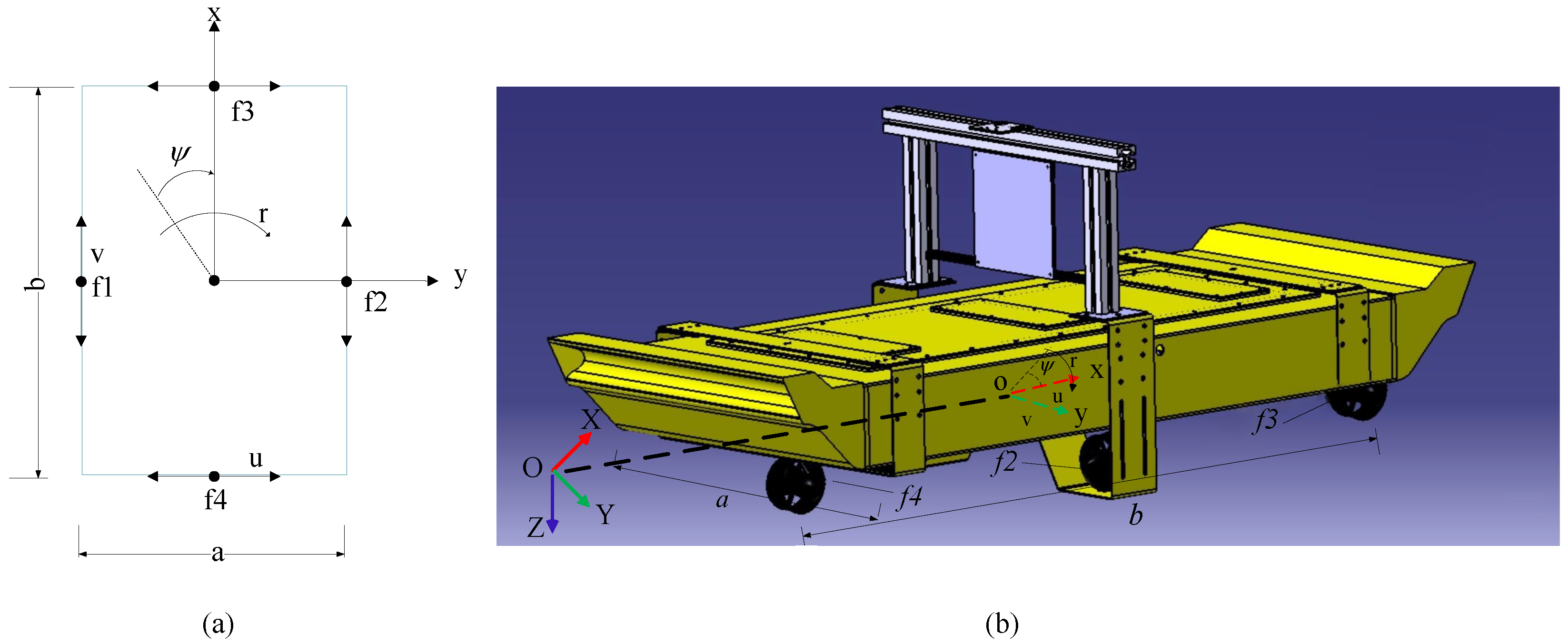
2.1. Design

In order to achieve high-efficiency propulsion for the USVs, the “+” shaped actuator configuration is adopted [30], as shown in Figure 1.

The shape of the USV is designed as a rectangle for easier docking, and its length and width are b and a, respectively. There are four propellers on the USV, namely $f1$, $f2$, $f3$, and $f4$, and they are fixed symmetrically. Among them, the direction of the thrusters’ force of $f1$ and $f2$ is along the x axis direction in the figure, and the direction of the thrusters’ force of $f3$ and $f4$ is depicted in the figure. The rear thruster and right thruster in Figure 1b correspond to $f4$ and $f2$ in Figure 1a, respectively.

2.2. Dynamics Model

The dynamics of our USV is described by the following nonlinear differential equation [31]:

$$\dot{\eta }=T\left(\eta \right)\nu$$

(1)

$$\dot{\nu }=M^{-1}BF-M^{-1}(C\left(\nu \right)+D\left(\nu \right))\nu$$

(2)

where $\eta ={[x,y,\psi ]}^T\in {\mathbb{R}}^{3\times 1}$, represents the longitudinal position, horizontal position, and the deflection angle of the USV in the inertial coordinate system. $\nu ={[u,v,r]}^T\in {\mathbb{R}}^{3\times 1}$ represents the velocity components of the three degrees of freedom of the USV, as shown in Figure 1. v represents the lateral speed of the USV, and u is the forward speed of the unmanned vessel. r is the yaw rate of the USV. $T\left(\eta \right)$ is the transformation matrix converting a state vector from the body frame to the inertial frame, which is described as

$$T\left(\eta \right)=\left[\begin{array}{ccc}cos\psi & -sin\psi & 0\\ sin\psi & cos\psi & 0\\ 0& 0& 1\end{array}\right]$$

(3)

$M\in {\mathbb{R}}^{3\times 3}$ is the positive definite symmetric mass inertia matrix, $C\left(\nu \right)\in {\mathbb{R}}^{3\times 3}$ is the centrifugal force matrix due to the rotation of the attached coordinate system. $D\left(\nu \right)\in {\mathbb{R}}^{3\times 3}$ is the positive semi-definite damping matrix. $M, C\left(\nu \right), D\left(\nu \right)$ are defined as

$$M=diag(m_{11},m_{22},m_{33})$$

(4)

$$C\left(\nu \right)=\left[\begin{array}{ccc}0& 0& -m_{22}v\\ 0& 0& m_{11}u\\ m_{22}v& -m_{11}u& -0\end{array}\right]$$

(5)

$$D=diag(X_u,Y_v,N_r)$$

(6)

where $m_{ii}(i=1,2,3)$ is the inertial mass with the additional mass and $X_u,Y_v,N_r$ are the hydrodynamic drag coefficients.

F$={[f1,f2,f3,f4]}^T$ represents the input control value of the entire dynamic model. Four of the forces represent the input of the left, right, front and rear thrusters, respectively, as shown in Figure 1. B is the control matrix describing the control sum of the thrusters, which is defined as

$$B=\left[\begin{array}{cccc}1& 1& 0& 0\\ 0& 0& 1& 1\\ {\displaystyle \frac{a}{2}}& {\displaystyle -\frac{a}{2}}& {\displaystyle \frac{b}{2}}& {\displaystyle -\frac{b}{2}}\end{array}\right]$$

(7)

where a is the distance of the transverse propeller, and b is the distance of the longitudinal propeller. Then, the three-degrees-of-freedom moment vector $\tau$ is finally defined as

$$\tau =B·F$$

(8)

According to Equations (1) and (2), it can be transformed into a non-linear state space expression, which is expressed as

$$\left\{\begin{array}{c}\dot{X}=f(X,F)\\ Y=g\left(X\right)\end{array}\right.$$

(9)

where $X={[x,y,\psi ,u,v,r]}^T$ is the state quantity of the system, and u is the force of the thrusters, which is the input of the system. $f:({\mathbb{R}}^6\times {\mathbb{R}}^4\to {\mathbb{R}}^6)$ is a nonlinear smooth function. The actual output positions of the USVs is given as follows

$$g\left(X\right)=\left[\begin{array}{cccccc}1& 0& 0& 0& 0& 0\\ 0& 1& 0& 0& 0& 0\\ 0& 0& 1& 0& 0& 0\end{array}\right]·X$$

(10)

3. Swarm Formation Control

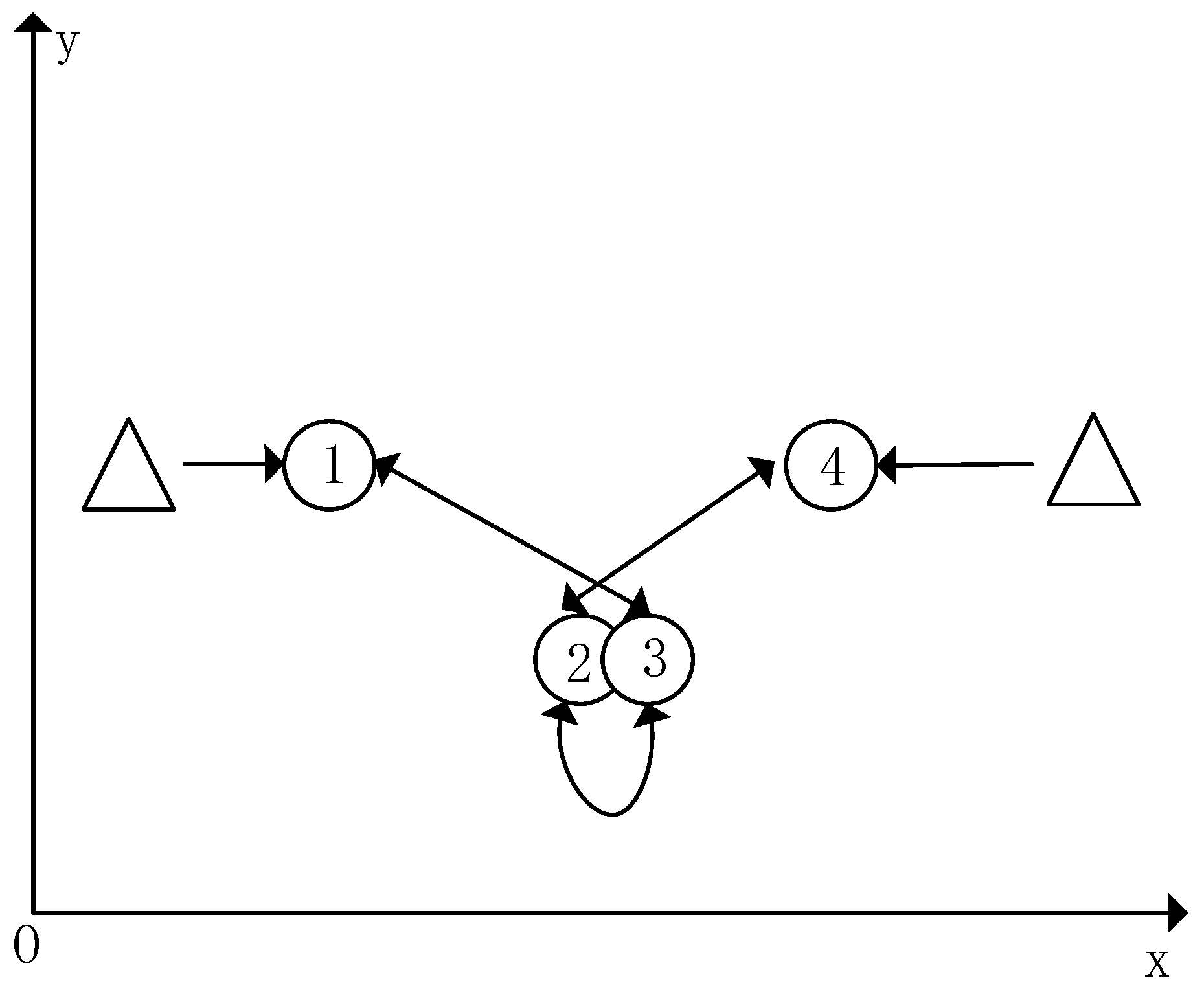
3.1. Formation Control Based on PDE

The purpose of this section is to accomplish the docking of multiple USVs in a line shape. Therefore, this paper adopts the complex-valued PDE method to model the dynamics of USVs. For a unit cell on a one-dimensional structure, $x(\alpha ,t)$ can be used to represent its position state, where $\alpha$ is the cell feature and t is the time. Therefore $x(\alpha ,t)$ represents the position of the unit cell $\alpha$ at time t. Based on formation control of multiple USVs in a 2D plane, the states of USVs can be given as follows

$$w(\alpha ,t)=x(\alpha ,t)+jy(\alpha ,t)$$

(11)

where w represents the position of the agent $\alpha$ at time t in two-dimensional space and $\alpha \in [0,1]$. If the USV in a multi-USVs system with $n+1$ agents are numbered, the i-th agent is expressed as

$$\alpha =\frac{i}{n}$$

(12)

where $i=0,1,2\cdots n$. The PDE-based kinetic model is shown as follows

$$w_t(\alpha ,t)=k(w_{\alpha \alpha }(\alpha ,t)-w_{\alpha \alpha }^d\left(\alpha \right))$$

(13)

$$w(0,t)=w^d\left(0\right)$$

(14)

$$w(1,t)=w^d\left(1\right)$$

(15)

where $w_t(\alpha ,t)$ indicates the first derivative of w with respect to t, and $w_{\alpha \alpha }(\alpha ,t)$ defines the second derivative of w with respect to $\alpha$. k is the gain constant. It is consistent with the law of the heat equation. $w^d\left(\alpha \right)$ is the position after the formation is completed, representing the desired shape that the agents would like to form. It can be seen from Equations (14) and (15) that $a_0$ and ${\alpha }_n$ are the boundaries of the reference formation trajectory and the leaders of the formation. The other agents are followers.

In order to apply the control rate to the limited USVs, the three-point central difference approximation method is selected to discretize the PDE model. As shown in Equation (12), a can be divided into $n+1$ points $\left\{0,1/n,2/n,\cdots ,1\right\}$. The interval step between points is $h=1/n$. The USVs on the boundary are the leaders indexed by $i=0$ and $i=n$, which set the position of the formation. The control laws for the leader are defined as follows

$$w_0\left(t\right)=w^d\left(0\right)$$

(16)

$$w_n\left(t\right)=w^d\left(1\right)$$

(17)

As is listed in Equations (16) and (17), the positioning of the formation is represented by $w_0$ and $w_n$. The control rate of the i-th USV as a follower is determined according to Equation (13) under the three-point central difference. The control rate of the i-th USV as a follower is

$$\begin{array}{c}\hfill {\dot{w}}_i=k\frac{w_{i+1}-w_i-(w_i-w_{i-1})}{h^2}-k\frac{w_{i+1}^d-w_i^d-(w_i^d-w_{i-1}^d)}{h^2}\end{array}$$

(18)

where $w_i=x_i\left(t\right)+j{y}_i\left(t\right)$ for the USV, and $i=1,2,3,\cdots ,n-1$. By using the control rate and anchor points, the USV follower can move once obtaining the relative position of its left neighbor and the relative position of its right neighbor i.e., $w_i-w_{i-1}$, $w_i^d-w_{i-1}^d$ and $w_{i+1}-w_i$, $w_{i+1}^d-w_i^d$. In the control rate, each follower should obtain the relative coordinates with its neighbors, and does not need the global coordinates and the specific positioning of the formation, so that the complex formation process can be completed at a relatively low cost.

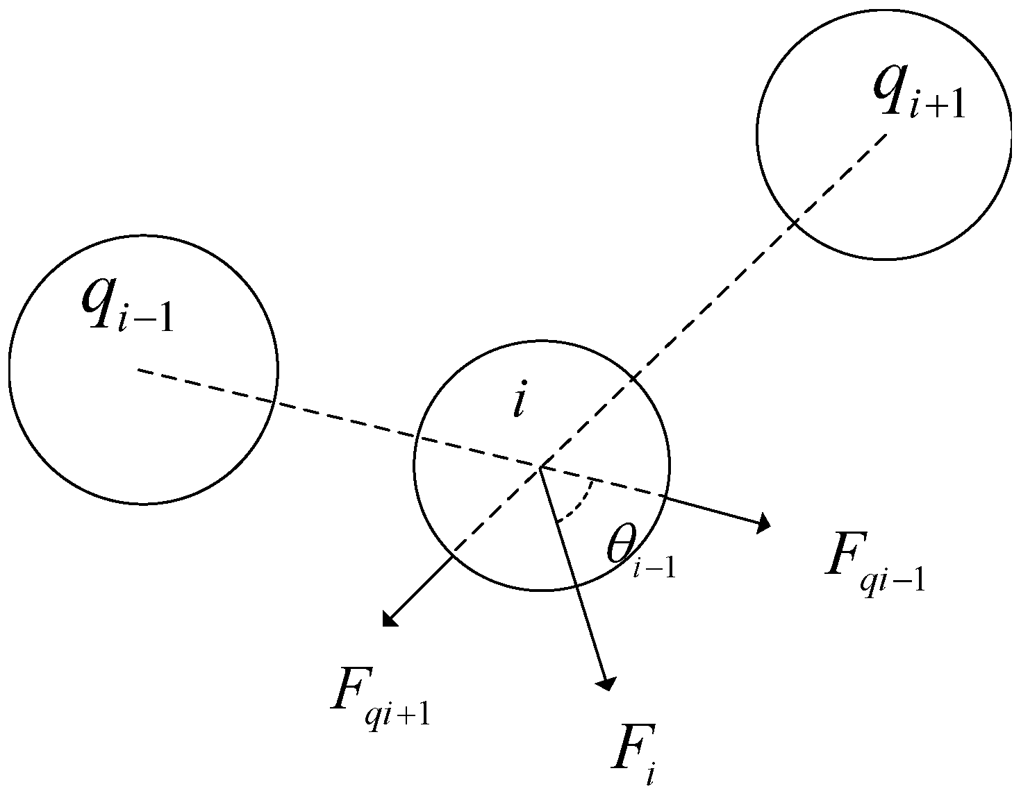
3.2. Formation Collision-Avoidance Control Based on Artificial Potential Field Method

According to Equation (18), the research object of the PDE method is the particle. However, the USV has a volume size in the real world. Regardless of the size of the USVs, collisions may occur as they are sailing in cross formation, as shown in Figure 2.

In Figure 2, the leader locates the position of the formation in the global domain, and the follower completes the line-formation movement according to the relative position information of the left and right neighbors in the PDE mode according to the number sequence. In order to avoid too complicated a single operation, independent modules and algorithms are employed to complete the collision-avoidance action.

The artificial potential field method is a planning algorithm that simulates the real physical field, and it is widely used in collision avoidance, path planning and other fields. It can convert the elements that affect the path planning into a simulated physical field. The controlled individual performs motion control by simulating the force of the entity in the physical field, so as to achieve the purpose of finding the optimal path. In the collision-avoidance algorithm, other robots are usually regarded as obstacles and simulated as repulsion field sources. The controlled individual can generate reverse acceleration through the appropriate repulsion function, when approaching other robots. In the collision-avoidance strategy, when the distance between the controlled individual and other robots is less than a certain distance, a high repulsion is generated. However, it has no effect on the USV outside the safe distance. The general repulsion function is shown as follows

$$U_q=\left\{\begin{array}{cccc}\frac{1}{2}\delta {(\frac{1}{D\left(q\right)}-\frac{1}{Q^{*}})}^2& ,D_q\le Q^{*}& & \\ \\ 0& ,D_q>Q^{*}& \end{array}\right.$$

(19)

$$F_q=-▿U_q=\left\{\begin{array}{cccc}\delta (\frac{1}{D\left(q\right)}-\frac{1}{Q^{*}})\frac{1}{D^2\left(q\right)}(▿D\left(q\right))& ,D_q\le Q^{*}& & \\ 0,& D_q>Q^{*}& \end{array}\right.$$

(20)

where q is the obstacle mark, and $\delta$ indicates the repulsion gain constant. $D\left(q\right)$ defines the distance between the controlled individual and the obstacle q. $Q^{*}$ represents the threshold of the repulsion action range. $U_q$ is the repulsion field received by the individual. The effect of the repulsion field can be adjusted by the value of $\delta$. Assuming that the controlled individual is the follower i, the repulsion exerted by the obstacle $q_{i-1}$ is $F_{q_{i-1}}$, and the relative angle is ${\theta }_{i-1}$. The resultant force of all obstacles on the controlled individual is denoted as $F_i$, which is shown in Figure 3.

Equation (21) represents the resultant force experienced by each USV in the formation.

$$\begin{array}{c}\hfill F_i=\left\{\begin{array}{cccc}{\displaystyle \sum _{m=1,m\ne i}^{n-1}}\delta (\frac{1}{D\left(q_m\right)}-\frac{1}{Q^{*}})\frac{1}{D^2\left(q_m\right)}(▿D\left(q_m\right))& ,D_{q_m}\le Q^{*}& & \\ \\ 0& ,D_{q_m}>Q^{*}& \end{array}\right.\end{array}$$

(21)

When multi-USVs choose the artificial potential field method to avoid collisions or obstacles in the formation control, the USVs and the obstacles may fall into a local minimum point, resulting in the agents being unable to fulfill the formation control. Thus, it will fall into a false equilibrium state. In order to avoid this situation, this paper adopts the additional rotating electric potential field force to release the false equilibrium state. As shown in Figure 4, the additional electric field force is

$$F_{di}=k_d\tau n$$

(22)

where $k_d$ is the gain of the additional rotating electric field force, ${\theta }_d\in (0,90)$ indicates the deflection angle of the additional rotating electric field force. $\tau =\left[\begin{array}{cc}cos{\theta }_d& -sin{\theta }_d\\ sin{\theta }_d& cos{\theta }_d\end{array}\right]$. n gives the direction in which the repulsion is pointing to.

The PDE formation collision-avoidance control rate based on artificial potential field method is shown below

$${\dot{w}}_i=k\frac{w_{i+1}-w_i-(w_i-w_{i-1})}{h^2}-k\frac{w_{i+1}^d-w_i^d-(w_i^d-w_{i-1}^d)}{h^2}+\beta F_i+\gamma F_{di}$$

(23)

where $\beta$ and $\gamma$ are the velocity gains of artificial repulsion and the additional rotational potential force, respectively.

4. Controller Design

In order to accomplish the USV docking, the controller should guide the vessel to a target point with the desired heading angle at a specific moment. Therefore, the reference trajectory is defined as the following

$$Y_r=g_r\left(X_r\right)$$

(24)

Subtracting Equation (24) from Equation (10), the system error can be defined as

$$E=[x_e,y_e,{\psi }_e]$$

(25)

Equation (25) is the difference between the planned position and the actual position of the USV at time t. In order to track the reference trajectory precisely, the following requirement should be met, ${\displaystyle \underset{t\to \infty }{lim}E=0}$.

4.1. Nonlinear Model Predictive Control

In the numerical simulation, Equation (9) is a continuous differential model, which cannot be directly used in the MPC controller to predict the state model. Considering that NMPC is applied in the actual situation, Equation (9) should be discretized, which is defined as follows

$$\left\{\begin{array}{c}x(n+1)=f_d(x\left(n\right),u\left(n\right))\\ \\ y\left(n\right)=g_d\left(x\left(n\right)\right)\end{array}\right.$$

(26)

where $f_d$ and $g_d$ are the discretized function. For the trajectory-tracking problem in the docking process of USVs, it is transformed into a constrained finite horizon nonlinear programming problem. At each simulation step length n, the trajectory-tracking error and the control effort should be close to optimal. In order to ensure that the USV can track the desired path accurately, the optimal control problem can be formulated as follows

$$\begin{array}{cc}\hfill minJ& {\displaystyle =\sum _{i=1}^{N_p}{∥(\widehat{y}(n+i)-y^{ref}(n+i))∥}_Q^2+\sum _{i=0}^{N_c}{∥\left(\widehat{u}(n+i)\right)∥}_R^2}\hfill \\ \hfill & s.t.\hfill \\ \hfill & y_{min}\le \widehat{y}(n+i)\le y_{max}\hfill \\ \hfill & u_{min}\le \widehat{u}(n+i)\le u_{max}\hfill \end{array}$$

(27)

where $N_p$ is the prediction horizon, and $N_c$ defines the control horizon. $y_{ref}\left(n\right)$ is the reference trajectory at the n-th step. $y_{ref}(n+i)$ is the reference trajectory at the $(n+i)$-th step. $\widehat{y}\left(n\right)$ gives the output result at the n-th time. $\widehat{y}(n+i)$ stands for the i-th prediction step at the n-th time. $\widehat{u}\left(n\right)$ is the input at time n-th and $\widehat{u}(n+i)$ denotes the prediction input of the i-th step at the n-th time. $y_{min}$ and $u_{min}$ represent the lower limit of output and control input, respectively. $y_{max},u_{max}$ represent the upper limit of output and control input, respectively. Q and R are the weighting matrices. Since $f_d$ is a non-linear function, the non-linear optimal solver is used to solve the optimization problem at the n-th time. In order to find the nonlinear optimal solution quickly [32], the non-linear solver of CasADi [33] is selected, and the multiple shooting method is used to speed up the solution process [34,35].

4.2. Iterative Learning-Based Model Predictive Control

Accurate and complete models are necessary in model predictive control. However, there exist external disturbances in the process of modeling and measurement, which make it difficult to establish an accurate model. When the USV is navigating on a water surface, it may be affected by the current and wind speed, where the dynamic model of the USV evolves. The dynamic equation is as defined as follow

$$\dot{\nu }=M^{-1}({\tau }_u+{\tau }_d)-M^{-1}(C\left(\nu \right)+D\left(\nu \right))\nu$$

(28)

where ${\tau }_u=B·F$ is the combined force of the USV controller, while ${\tau }_d$ is the combined force of wind and water.

When the USV is docking for the first time, the docking may fail due to the influence of the trajectory error. The USV then returns to the original origin for the second docking, and iterative learning is used to reduce docking errors. Iterative learning control is a data-driven method. The accurate mathematical model is not always necessary. It can adjust the control law parameters based on the previous control experience, so that the output result of the controlled object gradually approaches the expected value. After multiple iterations, the output tracks the setting value accurately. However, iterative learning control is not applicable to the common constraint problems of multivariable systems. The model predictive control can address the multivariate and constraint requirements of intermittent processes, and iterative learning control show good effects in repetitive control process. Thus, it is possible to combine the model predictive control with the iterative learning control during USV docking.

As is mentioned earlier, the goal of ILC is to design a learning algorithm to achieve high-quality tracking of trajectories, which enables the tracked trajectories to converge asymptotically along the batch iteration axis. In addition, the MPC strategy on the time axis is used to achieve better tracking performance and robustness against disturbances and uncertainties. The objective function of IMPC can be defined as follows

$$\begin{array}{cc}\hfill min{J}_k& {\displaystyle =\sum _{i=1}^{N_p}{∥({\widehat{y}}_k(n+i)-y^{ref}(n+i)+e_k(n+i))∥}_Q^2+\sum _{i=0}^{N_c}{∥\left({\widehat{u}}_k(n+i)\right)∥}_R^2}\hfill \\ \hfill & s.t.\hfill \\ \hfill & e_k\left(n\right)=\sum _{m=1}^{k-1}({\widehat{y}}_m\left(n\right)-y^{ref}\left(n\right))\hfill \\ \hfill & y_{min}\le \widehat{y}(n+i)\le y_{max}\hfill \\ \hfill & u_{min}\le \widehat{u}(n+i)\le u_{max}\hfill \end{array}$$

(29)

where $e_k\left(n\right)$ represents the error from the expected trajectory during the last iteration at the n-th time, and k represents the k-th iteration. In the first iteration step, there is no reference to the previous iteration process, so the error of the iteration batch is recorded starting from $k=2$. ${\widehat{y}}_k(n+i)$ represents the predicted output value in the k-th iteration. ${\widehat{u}}_k(n+i)$ represents the predicted input value in the k-th iteration, containing two inputs, which can be expressed by the following equation

$${\widehat{u}}_k\left(t\right)=u_k^{mpc}+u_k^{ILC}$$

(30)

According to the above optimal objective function, the block diagram of the iterative learning model predictive control is shown as follow in Figure 5.

In Figure 5, the module of “ILC Memory” is a storage module in the iterative process, which records the observation data of each time in the last iteration process. In the next iteration, the difference between the obtained data from the previous iteration and the expected data is used to compensate for the subsequent iteration. $e_k\left(n\right)$ represents the sum of errors at each moment in the previous $k-1$ iteration. $u_k\left(n\right)$ represents the control input at moment n in the k-th iteration. ${\widehat{y}}_k\left(n\right)$ gives the output value at the n-th moment in the k-th iteration. $y^{ref}\left(n\right)$ defines the reference value of the trajectory at the n-th moment, and the reference trajectory is consistent during each iteration.

5. Numerical Simulation

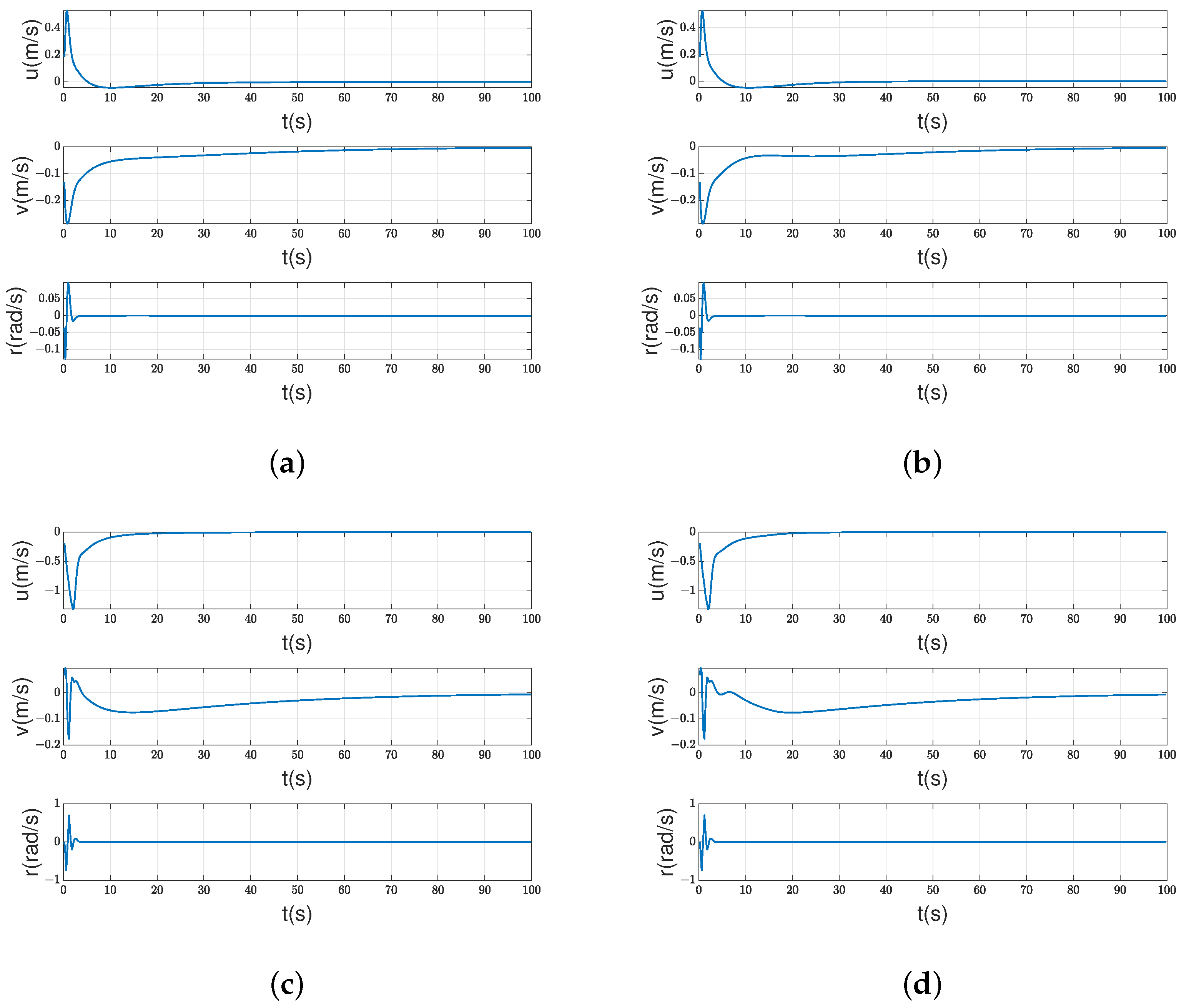
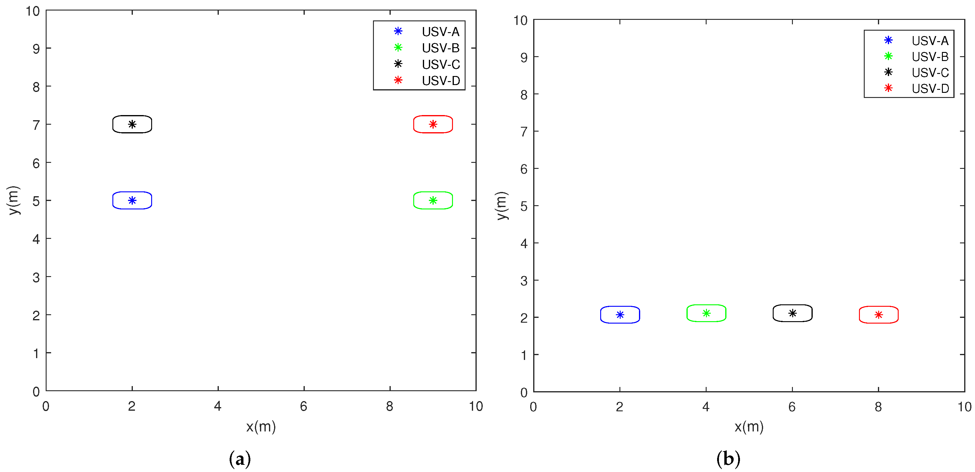
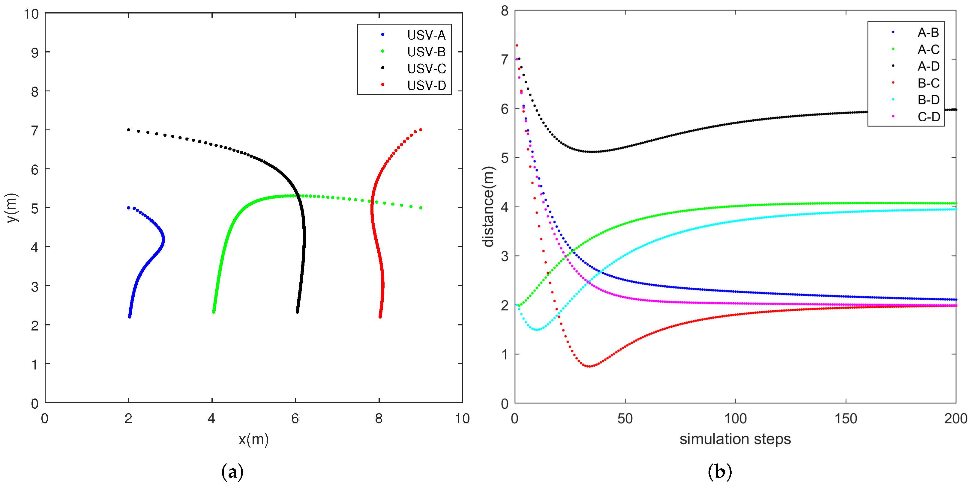
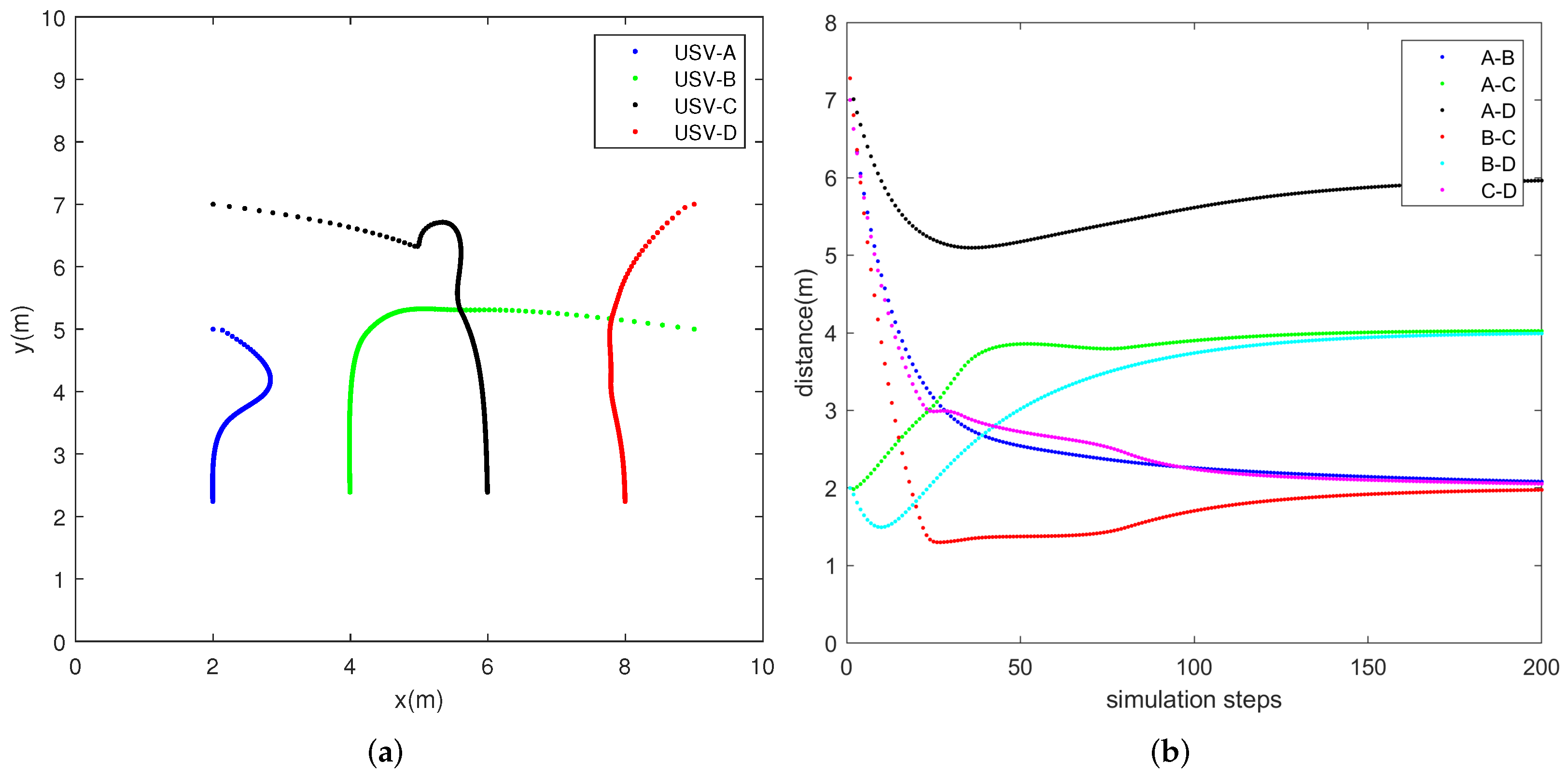
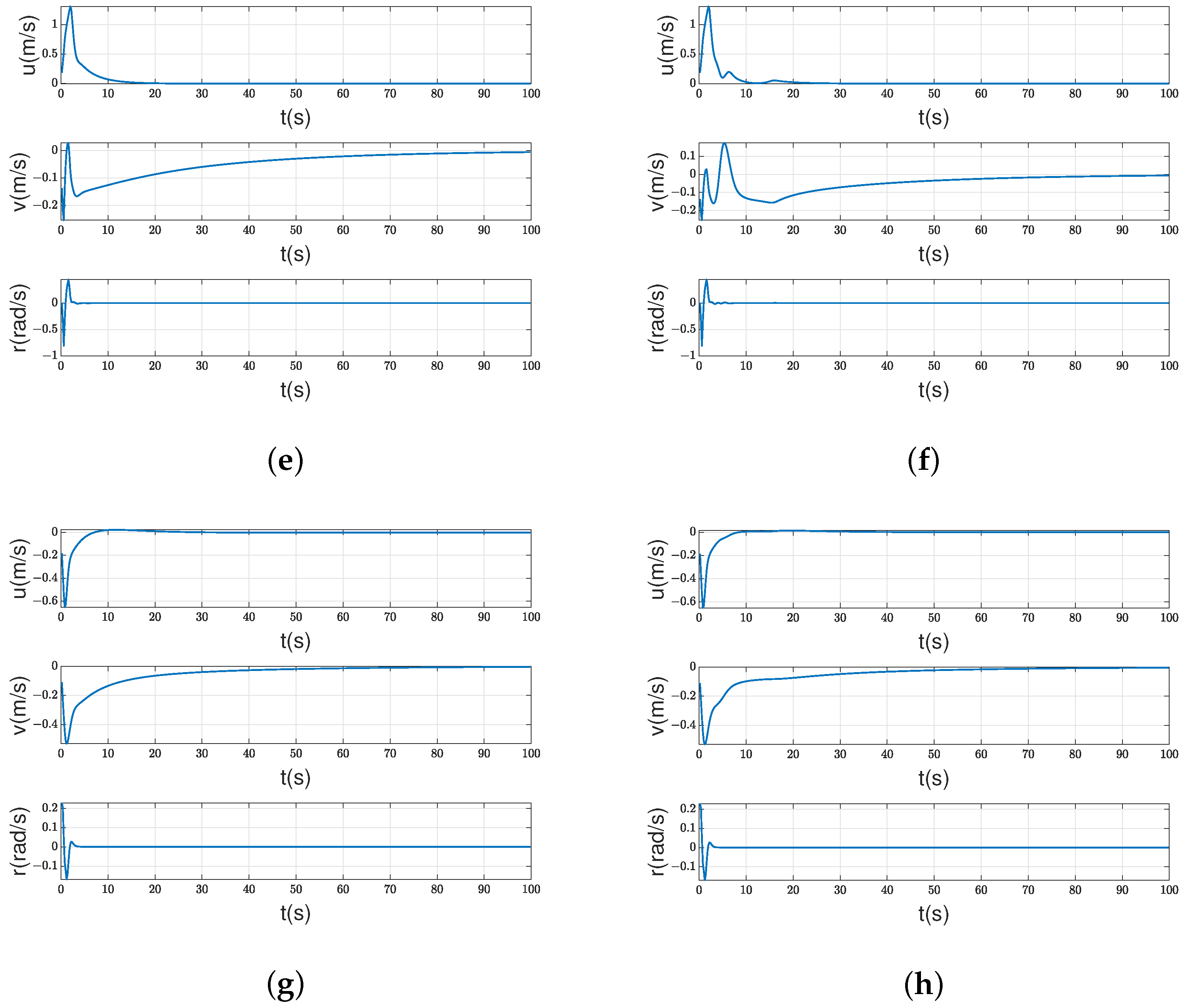
5.1. Formation Simulation

In this section, two simulation examples, i.e., clusters of USVs complete a line-shaped formation and the trajectory tracking of the USV docking process.

In order to evaluate the distributed control rate of formation tracking and obtain the line-shaped formation of USVs, the simulation is completed with four USVs. The control gain k of the formation is $0.07$. The expected formation curve is $u^d=10\ast \alpha +2\ast j$. The safe distance of the center of mass between USVs is set to 1 m. Repulsion influence radius $Q^{*}$ is 1.5 m. Repulsion gain constant $\delta$ is 1. The velocity gain $\beta$ of the repulsive force is 0.08. The velocity gain $\gamma$ of the additional rotating potential field force is 0.08. The initial and final positions of the USVs are shown in the Figure 6. Figure 7 describes the trajectories of USVs during the formation process, as well as the distance changes between USVs during the line-shaped formation process with the PDE formation control rate and without collision avoidance. When the artificial potential field method is not working, the formation movement process of USVs under the control rate of PDE can be treated as the movement of particles, but this does not consider the size of USV in the real world. When the number of iterations is from the 27-th to the 44-th step, the distance between USV-B and USV-C is less than 1 m, which is less than the safe distance. In order to address the collision problem in the process of USVs completing straight-line-shaped formations under the control rate of PDE in the real world, the superposition of the artificial potential field and PDE approach is proposed during formation of USVs. Figure 8 depicts the trajectory diagram of USVs during the formation process and the distance change diagram between individual USVs under the superposition of PDE control rate and artificial potential field. When USV-C detects that USV-B has entered the influence range of its own repulsion force, it will move in the opposite direction to USV-B under the action of the artificial repulsion force field.

In Figure 8, it can be clearly seen that USV-C has an obvious avoidance action at coordinate $(5,6)$, and the distance between USV-C and USV-B is always greater than 1 m. Figure 9 shows the velocity responses of the USVs under formation path planning in Figure 7 and Figure 8. Figure 9e,f demonstrates that the transverse velocity of USV-C has an obvious reverse change at $t=3$ s, which verifies that the avoidance is successful.

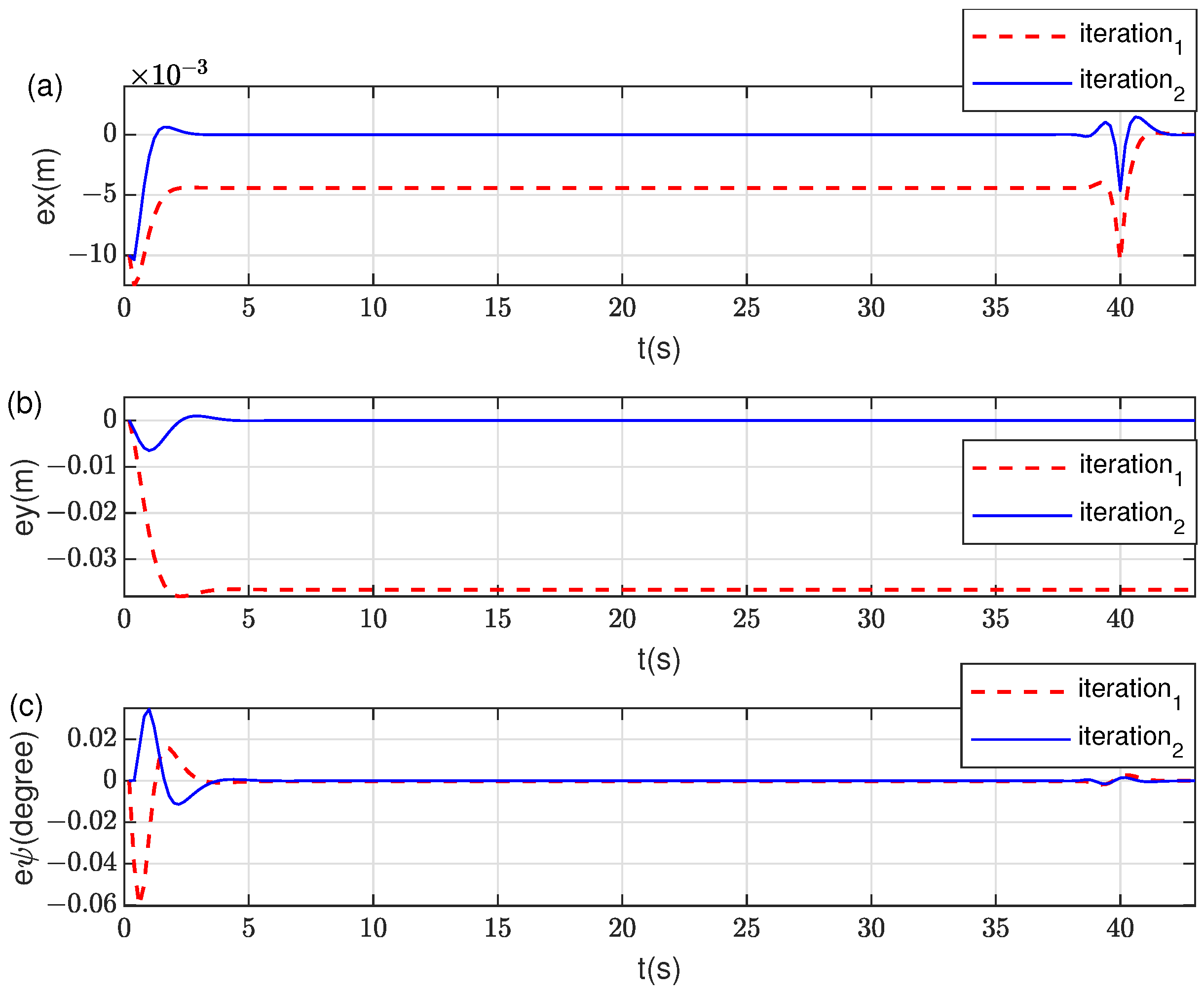
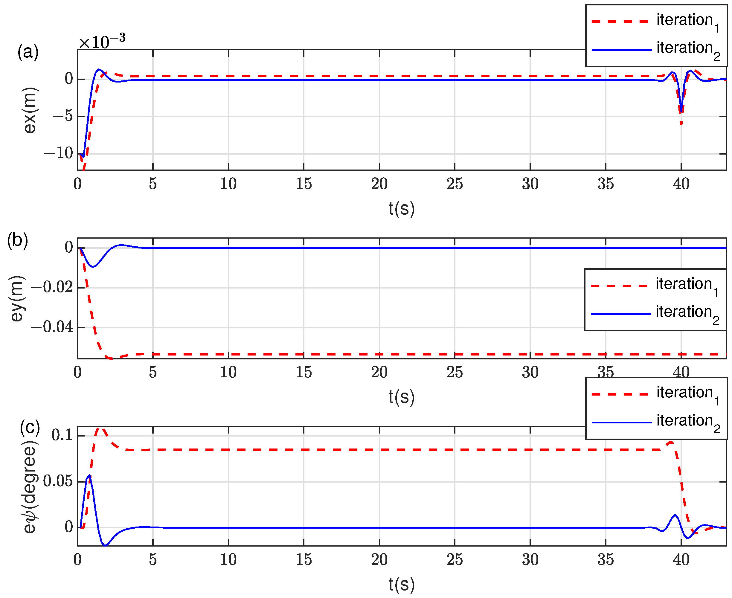
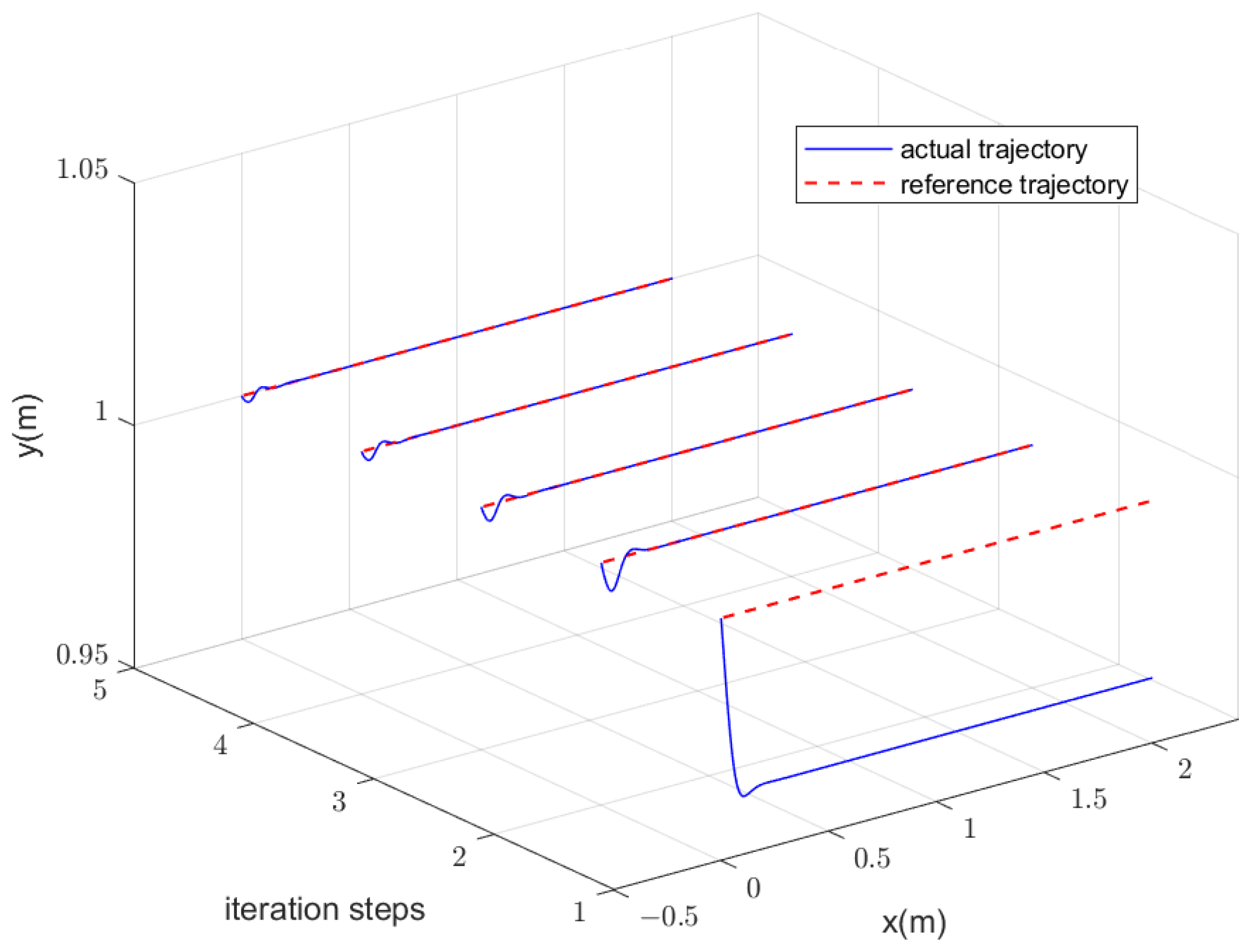
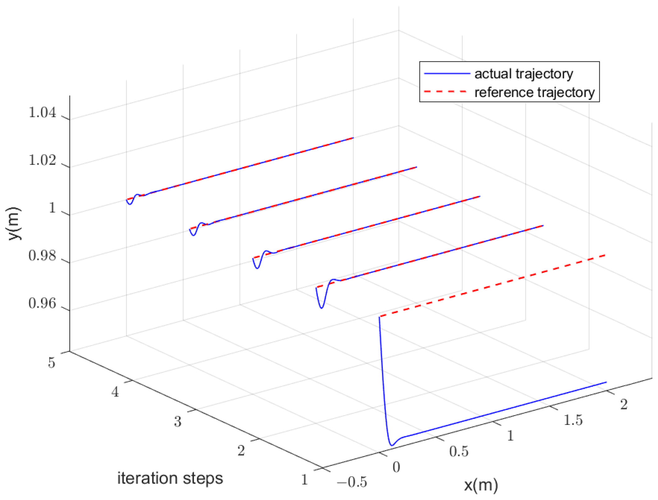
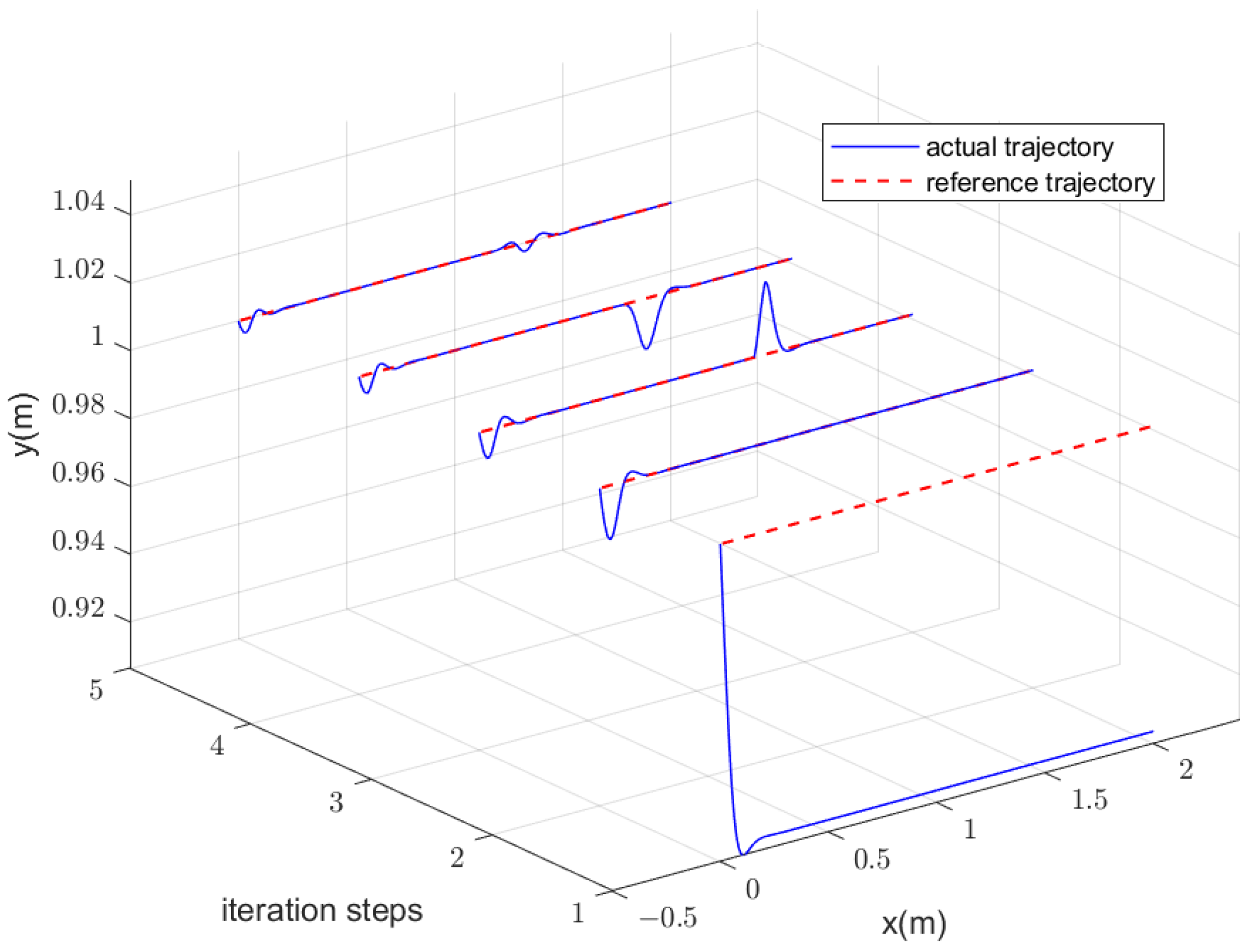
5.2. Iterative Docking Simulation

The parameters of the model are set as follows: $a=0.45$m, $b=0.9$m, $m_{11}=12.982$, $m_{22}=33.318$, $m_{33}=1.273$, $X_u=6.012$, $Y_v=7.112$, $N_r=0.771$. The weight parameter of the objective function is $Q=diag\left\{50,50,10\right\}$, $R=diag\left\{0.01,0.01,0.01,0.01\right\}$. The prediction interval $N_p$ is set to 10 and $N_c$ is set to 9. Sampling time T is $0.2$ s. The constraints of the thrusters are $-6N\le f_i\le 6N(i=1,2,3,4)$. The purpose of this paper is that USVs perform an autonomous docking process while completing a line-shaped formation. In an ideal straight-line-shaped formation, the trajectory of the docking is a point-to-point straight line. The initial and the final positions of the expected line are $(0,1)$, $(2,0)$, respectively.

Figure 10, Figure 11, Figure 12, Figure 13, Figure 14 and Figure 15 depict the comparative results of iterative tracking of USVs under various perturbations. The first iterations run under the MPC only, and subsequent iterations run under the ILMPC. In Figure 10, Figure 12 and Figure 14, the number of iterations increases sequentially from right to left. Figure 10 and Figure 11 are the tracking results and the error plots with model mismatch. To highlight the role of ILMPC, the model parameter $X_u$ is modified to $0.1$, and the lateral position deviation of the USV prediction model is set to 4 cm. At the first iteration, the trajectory-tracking steady-state error of USV in the longitudinal direction is about 5 mm, while the lateral position deviation is $3.6$ cm. When the USV unit reaches the target point at $t=40$ s, there is a little deviation in the longitudinal position of the USV due to the constraints of the control input. Under the action of ILMPC, in the second iteration, the USV can track the expected curve well. Figure 12 shows the iterative process of the USV under the disturbance of continuous wind speed and water flow, where the direction of wind speed and water flow is the direction of the transverse axis of the USV. The USV mostly deviates from the desired curve during the first iteration. In Figure 13, during the first iteration, the USV deviates from the desired lateral distance by $5.3$ cm, with a heading angle error of $0.085$ degrees. Under the action of iterative learning, the error is eliminated after the second iteration. In Figure 14 and Figure 15, it not only considers the disturbances such as model imbalance, continuous wind speed and water flow, but an instantaneous disturbance during the iteration is also added. During the first iteration, the USV had a longitudinal deviation of $4.3$ mm, a lateral deviation of $8.9$ cm, and a deviation of the heading angle of $0.1$ degrees. With the support of iterative learning, the expected curve can be tracked in the second iterative tracking process. The effects of random disturbances were not considered in the previous iterations. In order to test the ability of the algorithm to handle real-time disturbances, starting from the third iteration at $t=25$ s, a unit-step disturbance signal is applied to the lateral state output of the system. The simulation results show that the USV can quickly recover to the set value after the fluctuation with the real-time compensation of the MPC after the instantaneous disturbance during the movement.

Figure 16 describes the process of a line-shaped formation of four USVs at random positions and docking in sequence. In Figure 16a, the dotted rectangle is the initial position of the USVs. The line formation was completed in the PDE and the collision between USVs was avoided under the action of the artificial potential field method. Figure 16b–d shows the sequential docking processes of USV-C, USV-B, and USV-A, respectively.

6. Conclusions

In this paper, a control scheme based on PDE formation control and iterative learning model prediction is proposed for the straight-line automatic docking task of multiple USVs. For formation control of multiple USVs, this paper uses the artificial potential field method on the basis of PDE to solve the collision-avoidance problem due to ignoring the size of the control body in the process of PDE formation. In the process of USV docking, the classic MPC controller cannot overcome the issue of model mismatch and continuous disturbance of wind speed and water flow, but the docking process is actually a repeatable trajectory-tracking problem. Therefore, in view of this characteristic, this paper combines iterative learning with MPC. Once the first docking fails, a second iterative docking is performed. Thus, the uncertainty of the model system and the disturbance of the water environment can be effectively compensated. Finally, the overall effectiveness and superiority of the proposed control scheme are illustrated by two simulation examples, namely the formation-based simulation example and the docking simulation example. In follow-up work, practical tests will be performed with USVs.

References

- Du, Z.; Wen, Y.; Xiao, C.; Huang, L.; Zhou, C.; Zhang, F. Trajectory-cell based method for the unmanned surface vehicle motion planning. Appl. Ocean Res. 2019, 86, 207–221. [Google Scholar] [CrossRef]
- Wang, W.; Gheneti, B.; Mateos, L.A.; Duarte, F.; Ratti, C.; Rus, D. Roboat: An autonomous surface vehicle for urban waterways. In Proceedings of the 2019 IEEE/RSJ International Conference on Intelligent Robots and Systems (IROS), The Venetian Macao, Macau, China, 3–8 November 2019; pp. 6340–6347. [Google Scholar]
- Liu, H.; Lin, Z.; Cao, M.; Wang, X.; Lü, J. Coordinate-free formation control of multi-agent systems using rooted graphs. Syst. Control Lett. 2018, 119, 8–15. [Google Scholar] [CrossRef]
- Verginis, C.K.; Nikou, A.; Dimarogonas, D.V. Robust formation control in SE (3) for tree-graph structures with prescribed transient and steady state performance. Automatica 2019, 103, 538–548. [Google Scholar] [CrossRef] [Green Version]
- Ebel, H.; Eberhard, P. A comparative look at two formation control approaches based on optimization and algebraic graph theory. Robot. Auton. Syst. 2021, 136, 103686. [Google Scholar] [CrossRef]
- Ran, D.; Chen, X.; Misra, A.K. Finite time coordinated formation control for spacecraft formation flying under directed communication topology. Acta Astronaut. 2017, 136, 125–136. [Google Scholar] [CrossRef]
- Guo, F.; Zhang, T.; Zhang, F.; Gao, L.; Wang, Z.; Zhang, S. Event-triggered coordinated attitude control for satellite formation under switching topology. Adv. Control Appl. Eng. Ind. Syst. 2020, 2, 1–13. [Google Scholar] [CrossRef]
- Xu, Y.; Luo, D.; Zhou, L.; Shao, J.; You, Y. A gain matrix approach for robust distributed 3D formation control with second order swarm systems. Sci. Sin. Technol. 2020, 50, 461–474. [Google Scholar]
- Sarlette, A.; Sepulchre, R. A PDE viewpoint on basic properties of coordination algorithms with symmetries. In Proceedings of the 48h IEEE Conference on Decision and Control (CDC) Held Jointly with 2009 28th Chinese Control Conference, Shanghai, China, 15–18 December 2009; pp. 5139–5144. [Google Scholar]
- Qi, J.; Pan, F.; Qi, J. A PDE approach to formation tracking control for multi-agent systems. In Proceedings of the 2015 34th Chinese Control Conference (CCC), Hangzhou, China, 28–30 July 2015; pp. 7136–7141. [Google Scholar]
- Chen, H.; Qi, J.; Dong, Y.; Zhong, S. Multi-Robot Formation Control And Implementation. In Proceedings of the 2021 40th Chinese Control Conference (CCC), Shanghai, China, 26–28 July 2021; pp. 879–884. [Google Scholar]
- Meurer, T.; Krstic, M. Nonlinear PDE–based motion planning for the formation control of mobile agents. IFAC Proc. Vol. 2010, 43, 599–604. [Google Scholar] [CrossRef]
- Freudenthaler, G.; Meurer, T. PDE-based multi-agent formation control using flatness and backstepping: Analysis, design and robot experiments. Automatica 2020, 115, 108897. [Google Scholar] [CrossRef] [Green Version]
- Breivik, M.; Loberg, J.E. A virtual target-based underway docking procedure for unmanned surface vehicles. IFAC Proc. Vol. 2011, 44, 13630–13635. [Google Scholar] [CrossRef] [Green Version]
- Yu, W.; Wang, J.; Tang, G.; Li, M.; Qiao, Y. Dual-attention-based optical terminal guidance for the recovery of unmanned surface vehicles. Ocean Eng. 2021, 239, 109852. [Google Scholar] [CrossRef]
- Xie, T.; Li, Y.; Jiang, Y.; Pang, S.; Wu, H. Turning circle based trajectory planning method of an underactuated AUV for the mobile docking mission. Ocean Eng. 2021, 236, 109546. [Google Scholar] [CrossRef]
- Liao, Y.; Jia, Z.; Zhang, W.; Jia, Q.; Li, Y. Layered berthing method and experiment of unmanned surface vehicle based on multiple constraints analysis. Appl. Ocean Res. 2019, 86, 47–60. [Google Scholar] [CrossRef]
- Martinsen, A.B.; Lekkas, A.M.; Gros, S. Autonomous docking using direct optimal control. IFAC-PapersOnLine 2019, 52, 97–102. [Google Scholar] [CrossRef]
- Jiang, T.; Yang, Y.; Chen, H.; Wang, X.; Zhang, D. Way-point tracking control of underactuated USV based on GPC path planning. In Proceedings of the International Conference on Intelligent Robotics and Applications; Springer: Berlin/Heidelberg, Germany, 2019; pp. 393–406. [Google Scholar]
- Dong, Z.; Wan, L.; Li, Y.; Liu, T.; Zhang, G. Trajectory tracking control of underactuated USV based on modified backstepping approach. Int. J. Nav. Archit. Ocean Eng. 2015, 7, 817–832. [Google Scholar] [CrossRef] [Green Version]
- Su, Y.; Wan, L.; Zhang, D.; Huang, F. An improved adaptive integral line-of-sight guidance law for unmanned surface vehicles with uncertainties. Appl. Ocean Res. 2021, 108, 102488. [Google Scholar] [CrossRef]
- Kinjo, L.M.; Wirtensohn, S.; Reuter, J.; Menard, T.; Gehan, O. Trajectory tracking of a fully-actuated surface vessel using nonlinear model predictive control. IFAC-PapersOnLine 2021, 54, 51–56. [Google Scholar] [CrossRef]
- Abdelaal, M.; Fränzle, M.; Hahn, A. Nonlinear Model Predictive Control for trajectory tracking and collision avoidance of underactuated vessels with disturbances. Ocean Eng. 2018, 160, 168–180. [Google Scholar] [CrossRef]
- Haseltalab, A.; Garofano, V.; van Pampus, M.; Negenborn, R.R. Model Predictive Trajectory Tracking Control and Thrust Allocation for Autonomous Vessels. IFAC-PapersOnLine 2020, 53, 14532–14538. [Google Scholar] [CrossRef]
- Zheng, H.; Negenborn, R.R.; Lodewijks, G. Trajectory tracking of autonomous vessels using model predictive control. IFAC Proc. Vol. 2014, 47, 8812–8818. [Google Scholar] [CrossRef] [Green Version]
- Abdelaal, M.; Fränzle, M.; Hahn, A. NMPC-based trajectory tracking and collison avoidance of underactuated vessels with elliptical ship domain. IFAC-PapersOnLine 2016, 49, 22–27. [Google Scholar] [CrossRef]
- Yang, Y.; Li, Q.; Zhang, J.; Xie, Y. Iterative learning-based path and speed profile optimization for an unmanned surface vehicle. Sensors 2020, 20, 439. [Google Scholar] [CrossRef] [PubMed] [Green Version]
- Xu, C.; Wei, X.; Liu, L.; Zhang, L.; Liu, S. Iterative Learning Based Output Feedback Path Following Control for Marine Surface Vessels. In Proceedings of the 2019 Chinese Control Conference (CCC), Guangzhou, China, 27–30 July 2019; pp. 727–732. [Google Scholar]
- Liu, L.; Wang, D.; Peng, Z. Cooperative dynamic positioning of multiple offshore vessels with persistent ocean disturbances via iterative learning. In Proceedings of the 33rd Chinese Control Conference, Nanjing, China, 28–30 July 2014; pp. 8699–8704. [Google Scholar]
- Wang, W.; Mateos, L.A.; Park, S.; Leoni, P.; Gheneti, B.; Duarte, F.; Ratti, C.; Rus, D. Design, modeling, and nonlinear model predictive tracking control of a novel autonomous surface vehicle. In Proceedings of the 2018 IEEE International Conference on Robotics and Automation (ICRA), Brisbane, Australia, 21–25 May 2018; pp. 6189–6196. [Google Scholar]
- Wang, W.; Shan, T.; Leoni, P.; Fernández-Gutiérrez, D.; Meyers, D.; Ratti, C.; Rus, D. Roboat II: A Novel Autonomous Surface Vessel for Urban Environments. In Proceedings of the 2020 IEEE/RSJ International Conference on Intelligent Robots and Systems (IROS), Las Vegas, NV, USA, 24 October 2020–24 January 2021; pp. 1740–1747. [Google Scholar]
- Mehrez, M.W.; Mann, G.K.; Gosine, R.G. An optimization based approach for relative localization and relative tracking control in multi-robot systems. J. Intell. Robot. Syst. 2017, 85, 385–408. [Google Scholar] [CrossRef]
- Andersson, J.A.; Gillis, J.; Horn, G.; Rawlings, J.B.; Diehl, M. CasADi: A software framework for nonlinear optimization and optimal control. Math. Program. Comput. 2019, 11, 1–36. [Google Scholar] [CrossRef]
- Morrison, D.D.; Riley, J.D.; Zancanaro, J.F. Multiple shooting method for two-point boundary value problems. Commun. ACM 1962, 5, 613–614. [Google Scholar] [CrossRef]
- Bock, H.G.; Plitt, K.J. A multiple shooting algorithm for direct solution of optimal control problems. IFAC Proc. Vol. 1984, 17, 1603–1608. [Google Scholar] [CrossRef]
Publisher’s Note: MDPI stays neutral with regard to jurisdictional claims in published maps and institutional affiliations. |
© 2022 by the authors. Licensee MDPI, Basel, Switzerland. This article is an open access article distributed under the terms and conditions of the Creative Commons Attribution (CC BY) license (https://creativecommons.org/licenses/by/4.0/).
Share and Cite
Zhou, Y.; Wu, N.; Yuan, H.; Pan, F.; Shan, Z.; Wu, C. PDE Formation and Iterative Docking Control of USVs for the Straight-Line-Shaped Mission. J. Mar. Sci. Eng. 2022, 10, 478. https://doi.org/10.3390/jmse10040478
Zhou Y, Wu N, Yuan H, Pan F, Shan Z, Wu C. PDE Formation and Iterative Docking Control of USVs for the Straight-Line-Shaped Mission. Journal of Marine Science and Engineering. 2022; 10(4):478. https://doi.org/10.3390/jmse10040478
Chicago/Turabian StyleZhou, Yusi, Nailong Wu, Haodong Yuan, Feng Pan, Zhiyong Shan, and Chao Wu. 2022. "PDE Formation and Iterative Docking Control of USVs for the Straight-Line-Shaped Mission" Journal of Marine Science and Engineering 10, no. 4: 478. https://doi.org/10.3390/jmse10040478
APA StyleZhou, Y., Wu, N., Yuan, H., Pan, F., Shan, Z., & Wu, C. (2022). PDE Formation and Iterative Docking Control of USVs for the Straight-Line-Shaped Mission. Journal of Marine Science and Engineering, 10(4), 478. https://doi.org/10.3390/jmse10040478