Effects of Seawater Acidification on Echinoid Adult Stage: A Review

Asnicar, Davide; Marin, Maria Gabriella

doi:10.3390/jmse10040477

Open AccessReview

Effects of Seawater Acidification on Echinoid Adult Stage: A Review

by

Davide Asnicar

^*

and

Maria Gabriella Marin

Department of Biology, University of Padova, 35121 Padova, Italy

^*

Author to whom correspondence should be addressed.

J. Mar. Sci. Eng. 2022, 10(4), 477; https://doi.org/10.3390/jmse10040477

Submission received: 4 February 2022 / Revised: 23 March 2022 / Accepted: 24 March 2022 / Published: 29 March 2022

(This article belongs to the Special Issue Responses of Marine Invertebrates to Ocean Acidification: From Molecules to Organism)

Download

Browse Figures

Versions Notes

Abstract

:

The continuous release of CO₂ in the atmosphere is increasing the acidity of seawater worldwide, and the pH is predicted to be reduced by ~0.4 units by 2100. Ocean acidification (OA) is changing the carbonate chemistry, jeopardizing the life of marine organisms, and in particular calcifying organisms. Because of their calcareous skeleton and limited ability to regulate the acid–base balance, echinoids are among the organisms most threatened by OA. In this review, 50 articles assessing the effects of seawater acidification on the echinoid adult stage have been collected and summarized, in order to identify the most important aspects to consider for future experiments. Most of the endpoints considered (i.e., related to calcification, physiology, behaviour and reproduction) were altered, highlighting how various and subtle the effects of pH reduction can be. In general terms, more than 43% of the endpoints were modified by low pH compared with the control condition. However, animals exposed in long-term experiments or resident in CO₂-vent systems showed acclimation capability. Moreover, the latitudinal range of animals’ distribution might explain some of the differences found among species. Therefore, future experiments should consider local variability, long-term exposure and multigenerational approaches to better assess OA effects on echinoids.

Keywords:

ocean acidification; echinoids; sea urchin; physiology; behaviour; calcification; respiration

1. Introduction

The usage of fossil fuels and deforestation are constantly emitting carbon dioxide (CO₂) into the atmosphere, increasing its concentration [1]. This is recognized to be the most important factor causing climate change. Oceans play an important role in mitigating the greenhouse effect caused by CO₂ [2]. They have absorbed around 30–40% of the anthropogenic carbon dioxide [3,4], making the effects on land and the atmosphere milder but threatening marine organisms. Higher temperature and deoxygenation are causing the migration of animals towards other, more suitable environments, causing disruptions at the community level. Other climate change drivers are sneakier, and harder for animals to avoid. The increase in CO₂ absorbed by the ocean, due to the disruption of the carbonate system and the increase in H⁺ in seawater [5], is slowly but steadily lowering the pH of the marine environment worldwide, causing ocean acidification (OA), which represents a problem to the marine biota [1,6,7]. Models (Intergovernmental Panel on Climate Change—IPCC, Representative Concentration Pathway RCP8.5) predict that the pH value of surface seawater will decrease by ~0.4 units by the end of this century if the CO₂ emissions continue in a “business-as-usual” scenario [1,8].

OA effects on marine biota have been studied broadly in the past decade, highlighting interspecific variability in the response to this stressor [9,10,11,12,13]. Different animals have different sensitivities towards stressors due to physiological, behavioural and reproductive differences, even within closely related groups [14,15]. For example, gut pH regulation was shown to differ in six Ambulacraria species and was correlated with different sensitivity to OA. In particular, the species with the best ability to regulate pH were the most sensitive towards acidification conditions in terms of both survival and growth [9].

Calcifying organisms are especially threatened by acidification, due to the reduction in calcium carbonate (CaCO₃) saturation and, therefore, bioavailability [7]. For example, the mortality rate of oceanic copepods increased by 50% when animals were exposed to a reduction of 0.2 pH units [16]. However, the range of tolerance to pH variations and calcium carbonate bioavailability can vary among calcifers. Echinoderms have a calcareous skeleton mainly constituted of aragonite and calcite (CaCO₃ crystal forms) with a high magnesium calcite (MgCO₃) content [17]. MgCO₃ solubility is higher than CaCO₃, resulting in increased vulnerability of echinoderms to OA [18,19]. This is particularly evident in the Echinoidea class since sea urchins are highly calcified.

Because of their important role as a keystone species and their high sensitivity and rapid response to environmental changes, echinoids have been extensively used as model species in ecology and ecotoxicology studies to assess the effects of different stressors in the context of climate change and pollution [20,21,22]. If we consider their anatomy, physiology and life cycle, they represent an ideal bioindicator for the ongoing OA [23].

In past decades, much effort was devoted to understanding the potential effects of OA on echinoids by experimentally lowering the seawater pH to one or multiple high pCO₂ scenarios. However, most of the studies did not consider the extent of pH variability experienced in the field by the studied animals. Coastal environments, differently from the open ocean, are subject to high physico-chemical variability, which can promote adaptive responses and different sensitivity to OA [24,25,26,27]. Overlooking the local variability may lead to misleading and contrasting results which are not useful to predict animal responses to future OA scenarios [24,27].

Since most of the articles considered in this review did not take into account local adaptation and local natural pH data on a long timescale, we will refer to the pH reduction as seawater acidification (SWA) instead of OA, as a more comprehensive term.

Here, we summarized the findings of laboratory and field experiments that considered the maintenance of adult sea urchins at low pH conditions or comparisons of sea urchin specimens collected outside and within CO₂ volcanic vent systems (i.e., naturally acidified environments). The aim of the present article is not only to update the findings reported in previous papers (e.g., [23]), but also to provide a particular focus on key aspects of the echinoid adult stage to be considered in more depth in future studies. The articles collected assess the effects of SWA on the traits of adults’ biology, such as calcification, physiology, behaviour and reproduction, without examining the gamete, larval and juvenile stages. Most studies on the SWA effect on sea urchins have been carried out using gametes and larvae, fewer have considered the juvenile stage, while a few dozen have focused on the effects on the adult stage.

To search for papers on the focal topics, a systematic literature research was carried out using Web of Science and Google Scholar databases, and the following keywords: “ocean acidification”, “seawater acidification”, “reduced pH”, “sea urchin”, “echinoid”, “adult”, “physiology”, “calcification”, “behaviour”, and “reproduction”, and their combinations. Studies where the OA conditions were achieved with other methods than CO₂ insufflation were excluded from the review.

From the survey of the literature, 50 papers (62 experiments in total; experiments within a paper are defined as exposures carried out with different species or different duration) were included in this review. In tables reported below, studies about calcification, physiology, behaviour and reproduction are listed. Most of the experiments examined multiple effects of decreased pH on the adult sea urchin biology (on average, 3–4 endpoints per article). A total of 29 experiments used only one condition of reduced pH (plus the control), while 23 used two reduced pH values and 9 used three reduced pH values. Of all the experiments, nine were conducted using animals resident in vent systems. Of all the studies exposing animals in the laboratory, 33% considered the pH changes that are predicted for the end of the present century or sooner (from 0.1 to 0.4 units of pH reduction). In total, 44% of the articles considered both a pH reduction in the range of 0.1–0.4 and more severe scenarios that might be reached by the end of the 24th century [1]. Other works (23%) tested only a pH reduction greater than −0.4 or a too-severe scenario that is unlikely to be reached (e.g., the case of [28,29] where the highest pH reduction compared with the control was −1.3 and −1.8 pH units). Most of the negative effects were found in studies where ΔpH was higher than 0.4; for each endpoint analysed, 25% and 61% of the biological responses obtained were worsened by SWA if ΔpH in the experiment was ≤0.4 and >0.4 units, respectively.

Although most studies have been carried out using species from either the subtropical–temperate (43%; e.g., Paracentrotus lividus, Heliocidaris erythrogramma, Hemicentrotus pulcherrimus) or the equatorial area (36%; e.g., Salmacis virgulata, Lythechinus variegatus, Echinometra sp.), the latitudinal range covered the whole globe, including subpolar–polar species (e.g., Strongylocentrotus droebachiensis, Sterechinus neumayeri; 15%) and also deep-sea species (Strongylocentrotus fragilis, 6%).

Among the studies considered, the vast majority of the endpoints focused on the calcification and physiology of the animals exposed to reduced pH.

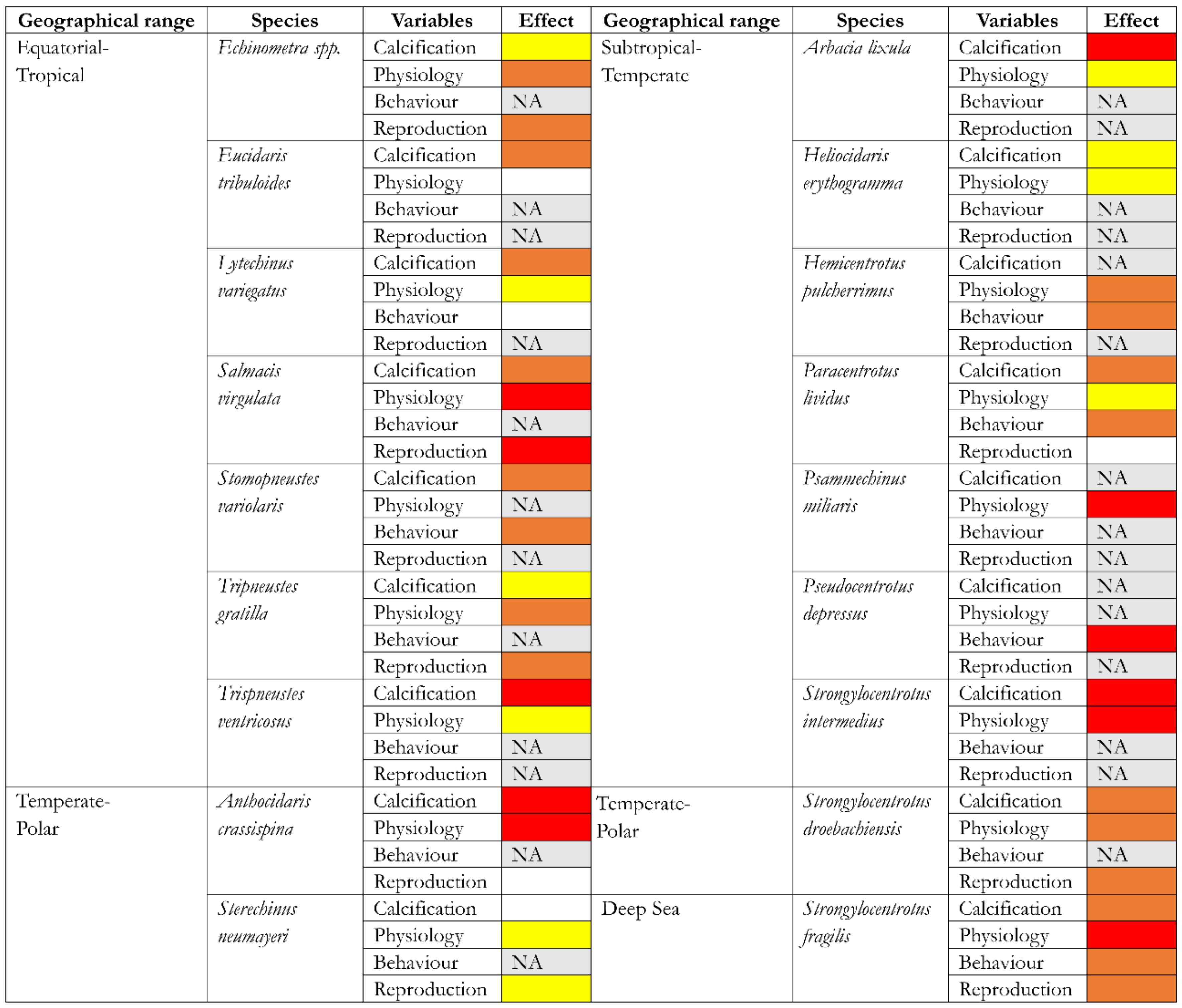
2. SWA Effects on Echinoid Calcification

The mineralogical composition of sea urchins varies greatly among species, but also among individuals and among different structures of each individual [30]. In most echinoids, approximately 4% calcite has magnesium ions that substitute calcium ions. Mg-calcite is more soluble than calcite and therefore, in relation to the high Mg content, the skeletal structures of echinoids are especially weakened in a more acidic environment [17,30,31,32,33]. The Mg-calcite content of sea urchin skeletal structures, and therefore their solubility in acidified conditions, vary with latitude, being higher in warmer waters [30]. In all the collected studies concerning test skeletal mineralogy and the related ability to tolerate mechanical stress (Table 1, line 39–69; 19 studies), 7 out of 12 species showed alterations due to low pH. Alterations were detected in both short-term and long-term exposure.

Table 1. List of studies performed on echinoid adult stage to investigate effects of SWA on calcification. “pH level” contains the value of all the conditions tested; the first value is the control. In the case that the same article tested both a realistic (ΔpH ≤ 0.4; based on IPCC RCP8.5) and unrealistic scenario (ΔpH > 0.4), the two conditions were split. Abbreviations: Eq.-Trop. = Equatorial–Tropical; Sub.-Temp. = Subtropical–Temperate; Temp.-Pol. = Temperate–Polar.

N	Response Detail	Species	Latitudinal Range	pH Level	ΔpH	Exposure Time (Days)	ΔpH Effect	Citation
1	Growth	Heliocidaris erythrogramma	Sub.-Temp.	8.1–7.8	0.3	14	=	[34]
2	Growth	Heliocidaris erythrogramma	Sub.-Temp.	8.1–7.6–7.4	0.5–0.7	14	=	[34]
3	Growth	Echinometra mathaei	Eq.-Trop.	8.04–7.69	0.35	49	=	[35]
4	Growth	Strongylocentrotus intermedius	Sub.-Temp.	8.10–7.82	0.28	60	Altered	[36]
5	Growth	Strongylocentrotus intermedius	Sub.-Temp.	8.10–7.68–7.55	0.42–0.55	60	Altered	[36]
6	Growth	Paracentrotus lividus	Sub.-Temp.	7.9–7.7	0.2	60	=	[37]
7	Growth	Paracentrotus lividus	Sub.-Temp.	7.9–7.4	0.5	60	Slower	[37]
8	Growth	Paracentrotus lividus	Sub.-Temp.	8.04–7.78	0.26	90	=	[38]
9	Growth	Strongylocentrotus fragilis	Deep Sea	7.92–7.64	0.28	140	=	[39]
10	Growth	Strongylocentrotus fragilis	Deep Sea	7.92–7.23–6.61	0.69–1.31	140	Altered	[39]
11	Growth	Anthocidaris crassispina	Temp.-Pol.	8.15–7.83	0.32	140	=	[40]
12	Growth	Anthocidaris crassispina	Temp.-Pol.	8.15–7.33	0.82	140	altered	[40]
13	Growth	Tripneustes gratilla	Eq.-Trop.	8.1–7.8	0.3	146	=	[41]
14	Growth	Tripneustes gratilla	Eq.-Trop.	8.1–7.6	0.5	146	Decreased	[41]
15	Growth	Echinometra mathaei	Eq.-Trop.	8.09–7.63	0.46	360	=	[42]
16	Growth	Echinometra sp.	Eq.-Trop.	8.06–7.89–7.79	0.17–0.27	600	=	[43]
17	Growth	Sterechinus neumayeri	Temp.-Pol.	7.98–7.72	0.26	1200	=	[44]
18	Growth	Sterechinus neumayeri	Temp.-Pol.	7.98–7.52	0.46	1200	=	[44]
19	Growth	Echinometra sp.	Eq.-Trop.	8.0–7.48	0.52	Resident	=	[45]
20	Growth	Echinometra sp.	Eq.-Trop.	8.0–7.48	0.52	Resident	Increase	[45]
21	Growth (jaw size)	Paracentrotus lividus	Sub.-Temp.	7.9–7.7	0.2	60	Decreased	[37]
22	Growth (jaw size)	Paracentrotus lividus	Sub.-Temp.	7.9–7.4	0.5	60	Decreased	[37]
23	Growth (ossicles)	Strongylocentrotus droebachiensis	Temp.-Pol.	8.00–7.66	0.34	42	Reduced	[46]
24	Growth (ossicles)	Strongylocentrotus droebachiensis	Temp.-Pol.	8.00–7.19	0.81	42	Reduced	[46]
25	Mineral ionic content	Paracentrotus lividus	Sub.-Temp.	8.06–7.69	0.37	1	Altered	[47]
26	Mineral ionic content	Arbacia lixula	Sub.-Temp.	8.06–7.69	0.37	1	Altered	[47]
27	Mineral ionic content	Paracentrotus lividus	Sub.-Temp.	8.05–7.73	0.32	4	Altered	[47]
28	Mineral ionic content	Arbacia lixula	Sub.-Temp.	8.05–7.73	0.32	4	=	[47]
29	Porosity	Heliocidaris erythogramma	Sub.-Temp.	8.01–7.6	0.39	210	=	[48]
30	Skeletal degradation	Eucidaris tribuloides	Eq.-Trop.	8.05–7.68	0.37	45	Higher (Spines)	[49]
31	Skeletal degradation	Eucidaris tribuloides	Eq.-Trop.	8.05–7.39	0.66	45	Higher (Spines)	[49]
32	Skeletal degradation	Tripneustes ventricosus	Eq.-Trop.	8.04–7.65	0.39	45	Higher (Spines)	[49]
33	Skeletal degradation	Tripneustes ventricosus	Eq.-Trop.	8.04–7.41	0.63	45	Higher (Spines)	[49]
34	Skeletal degradation	Paracentrotus lividus	Sub.-Temp.	8.11–7.75–7.50–7.48	0.36–0.61–0.63	Resident	Higher	[50]
35	Skeletal degradation	Arbacia lixula	Sub.-Temp.	8.11–7.75–7.50–7.48	0.36–0.61–0.63	Resident	Higher	[50]
36	Skeletal integrity	Echinometra sp.	Eq.-Trop.	8.1–7.7	0.4	330	=	[51]
37	Skeletal integrity	Paracentrotus lividus	Sub.-Temp.	7.93–7.63	0.3	Resident	=	[52]
38	Skeletal integrity	Arbacia lixula	Sub.-Temp.	7.93–7.63	0.3	Resident	Lowered	[52]
39	Skeletal mechanical properties	Paracentrotus lividus	Sub.-Temp.	8.0–7.8–7.7	0.2–0.3	30	=	[53]
40	Skeletal mechanical properties	Strongylocentrotus droebachiensis	Temp.-Pol.	8.00–7.66	0.34	42	=	[46]
41	Skeletal mechanical properties	Strongylocentrotus droebachiensis	Temp.-Pol.	8.00–7.19	0.81	42	Lower force and high dissolution	[46]
42	Skeletal mechanical properties	Tripneustes gratilla	Eq.-Trop.	8.1–7.8	0.3	146	=	[54]
43	Skeletal mechanical properties	Tripneustes gratilla	Eq.-Trop.	8.1–7.6	0.5	146	Decreased	[54]
44	Skeletal mechanical properties	Heliocidaris erythogramma	Sub.-Temp.	8.01–7.6	0.39	210	=	[48]
45	Skeletal mechanical properties	Echinometra mathaei	Eq.-Trop.	8.09–7.63	0.46	360	=	[42]
46	Skeletal mechanical properties	Paracentrotus lividus	Sub.-Temp.	8.0–7.9–7.8	0.1–0.2	360	=	[55]
47	Skeletal mechanical properties	Paracentrotus lividus	Sub.-Temp.	8.02–7.865–7.65	0.155–0.37	Resident	=	[55]
48	Skeletal mechanical properties	Paracentrotus lividus	Sub.-Temp.	8.1–7.8	0.3	Resident	=	[55]
49	Skeletal mechanical properties	Paracentrotus lividus	Sub.-Temp.	7.93–7.63	0.3	Resident	=	[52]
50	Skeletal mechanical properties	Arbacia lixula	Sub.-Temp.	7.93–7.63	0.3	Resident	Altered	[52]
51	Skeletal mechanical properties	Sterechinus neumayeri	Temp.-Pol.	8.1–7.8	0.3	Resident	=	[56]
52	Skeletal mineralogy	Strongylocentrotus droebachiensis	Temp.-Pol.	8.00–7.66	0.34	42	=	[46]
53	Skeletal mineralogy	Strongylocentrotus droebachiensis	Temp.-Pol.	8.00–7.19	0.81	42	Dissolution	[46]
54	Skeletal mineralogy	Echinometra sp.	Eq.-Trop.	8.1–7.9	0.2	70	=	[57]
55	Skeletal mineralogy	Tripneustes gratilla	Eq.-Trop.	8.1–7.8	0.3	146	=	[54]
56	Skeletal mineralogy	Tripneustes gratilla	Eq.-Trop.	8.1–7.6	0.5	146	=	[54]
57	Skeletal mineralogy	Paracentrotus lividus	Sub.-Temp.	8.02–7.8	0.18	Resident	=	[58]
58	Skeletal mineralogy (Aristotle’s lantern)	Anthocidaris crassispina	Temp.-Pol.	8.15–7.83	0.32	140	Thinner	[40]
59	Skeletal mineralogy (Aristotle’s lantern)	Anthocidaris crassispina	Temp.-Pol.	8.15–7.33	0.82	140	Thinner	[40]
60	Skeletal mineralogy (FTIR-TGA)	Salmacis virgulata	Eq.-Trop.	8.26–8.00	0.26	14	=	[59]
61	Skeletal mineralogy (FTIR-TGA)	Salmacis virgulata	Eq.-Trop.	8.26–7.81–7.63	0.45–0.63	14	Loss of weight, less calcite	[59]
62	Skeletal mineralogy (gene expr.)	Lytechinus variegatus	Eq.-Trop.	7.93–7.7	0.23	56	=	[60]
63	Skeletal mineralogy (gene expr.)	Lytechinus variegatus	Eq.-Trop.	7.93–7.47	0.46	56	Upregulated	[60]
64	Skeletal mineralogy (gene expr.)	Paracentrotus lividus	Sub.-Temp.	7.93–7.63	0.3	Resident	=	[52]
65	Skeletal mineralogy (gene expr.)	Arbacia lixula	Sub.-Temp.	7.93–7.63	0.3	Resident	Altered	[52]
66	Skeletal mineralogy (Mg, Sr, Ca)	Stomopneustes variolaris	Eq.-Trop.	7.96–7.76	0.2	210	=	[61]
67	Skeletal mineralogy (Mg, Sr, Ca)	Stomopneustes variolaris	Eq.-Trop.	7.96–7.46	0.5	210	Altered	[61]
68	Skeletal mineralogy (Mn, Sr, Zn)	Paracentrotus lividus	Sub.-Temp.	8.11–7.75–7.50–7.48	0.36–0.61–0.63	Resident	Altered	[50]
69	Skeletal mineralogy (Mn, Sr, Zn)	Arbacia lixula	Sub.-Temp.	8.11–7.75–7.50–7.48	0.36–0.61–0.63	Resident	Altered	[50]
70	Spine development	Heliocidaris erythrogramma	Sub.-Temp.	8.1–7.8	0.3	14	=	[34]
71	Spine development	Heliocidaris erythrogramma	Sub.-Temp.	8.1–7.6–7.4	0.5–0.7	14	Impaired	[34]
72	Spine development	Lytechinus variegatus	Eq.-Trop.	7.93–7.7	0.23	56	=	[60]
73	Spine development	Lytechinus variegatus	Eq.-Trop.	7.93–7.47	0.46	56	Impaired	[60]
74	Spine length	Paracentrotus lividus	Sub.-Temp.	8.04–7.78	0.26	90	Decreased	[38]
75	Spine mechanical strength	Eucidaris tribuloides	Eq.-Trop.	8.05–7.68	0.37	45	=	[49]
76	Spine mechanical strength	Eucidaris tribuloides	Eq.-Trop.	8.05–7.39	0.66	45	=	[49]
77	Spine mechanical strength	Tripneustes ventricosus	Eq.-Trop.	8.04–7.65	0.39	45	=	[49]
78	Spine mechanical strength	Tripneustes ventricosus	Eq.-Trop.	8.04–7.41	0.63	45	Decreased	[49]
79	Spine tips integrity	Heliocidaris erythrogramma	Sub.-Temp.	8.1–7.8	0.3	14	=	[34]
80	Spine tips integrity	Heliocidaris erythrogramma	Sub.-Temp.	8.1–7.6–7.4	0.5–0.7	14	Dissolved (7,4)	[34]
81	Spines integrity	Stomopneustes variolaris	Eq.-Trop.	7.96–7.76	0.2	210	=	[61]
82	Spines integrity	Stomopneustes variolaris	Eq.-Trop.	7.96–7.46	0.5	210	Reduced	[61]
83	Test robustness	Paracentrotus lividus	Sub.-Temp.	8.04–7.78	0.26	90	=	[38]
84	Test thickness	Paracentrotus lividus	Sub.-Temp.	8.04–7.78	0.26	90	Thinner	[38]
85	Test thickness	Tripneustes gratilla	Eq.-Trop.	8.1–7.8	0.3	146	=	[54]
86	Test thickness	Tripneustes gratilla	Eq.-Trop.	8.1–7.6	0.5	146	Decreased	[54]

S. virgulata, exposed at a pH reduced by 0.4 and 0.6 units [59], after 14 days had less calcite and lost weight. S. droebachiensis instead showed traces of carbonate dissolution after 42 days, but only at the greatest ΔpH (0.81 compared with control) [46]. In the other four species subjected to longer exposures (from 56 days up to being resident in vent systems), low pH conditions did not cause a variation in the calcification (Table 1). Only one case of long exposure (146 days) to reduced pH resulted in decreased mechanical properties of the T. gratilla skeleton. The force needed to break the sea urchin test was lower if animals were maintained at low pH compared with those at pH 8.1. However, the effect of SWA was significant only if the ΔpH was −0.5 units, and not in the case of 0.3 [54].

Alterations in calcification were present also in animals resident in CO₂ vents. Differences in the element composition were found in P. lividus and A. lixula specimens sampled in volcanic vent systems in the Mediterranean Sea. In particular, in the test of animals sampled in three acidified sites (ΔpH 0.36, 0.61 and 0.63 compared with the control site, pH 8.11), manganese and strontium contents were significantly higher, whereas zinc content was significantly lower [50]. Those specimens also suffered higher skeletal degradation with microfractures visible using scanning electron microscopy. Species-specific differences were found, with more severe effects in P. lividus than A. lixula [50]. However, the effect of local variability is a key point that must be considered in the response of calcification to SWA. Indeed, a similar study performed in another volcanic vent system in the Mediterranean Sea (local pH 7.63, reduced by 0.3 units compared with the control site) showed that A. lixula was more sensitive to SWA than P. lividus. Alterations in the gene expression were associated with decreased mechanical properties of the spines and test in A. lixula [52]. Nonetheless, in both studies, A. lixula maintained higher abundance in the vent sites compared with P. lividus [50,52]. This suggested that other factors were involved in the maintenance of the populations (e.g., larval plasticity influencing the settlement).

The duration of exposure to SWA has major relevance to the occurrence of skeletal mineralogy changes. This suggests that echinoids can maintain active calcification processes, making the carbonate bioavailability stable [57]. In addition, SWA effects are negligible in the case that the ΔpH is smaller than 0.4, and are usually more severe when ΔpH is greater than 0.4 units. For example, the sea urchin S. variolaris kept for 210 days at a pH reduced by 0.2 units did not show effects on the skeletal mineralogy and the spine integrity. However, if specimens were kept at a pH reduction of 0.5 units, the skeletal characteristics varied significantly compared with the control [61]. In the study of Dery and colleagues, traces of corrosion were highlighted in Eucidaris tribuloides exposed to pH 7.4 for 45 days, whereas no effects were observed at pH 7.7 [49]. Several experiments demonstrated that the prolongation of the exposure can lead to an improvement in the condition, resulting in a decreased acidification impact. The reduction in calcium carbonate saturation in seawater can be compensated for by modulating gene expression, as reported by Emerson and colleagues [60]. Indeed, Lytechinus variegatus exposed to pH 7.7 and 7.47 for 56 days showed impairment in the development of spines but the genes involved in the regeneration process were upregulated. This suggested that, with time, those animals would have been able to face SWA [60].

The difficulty of building calcareous structures in an acidified environment can lead to impairment in the growth of the skeletal parts of echinoids (test, jaws, and spines). This was the case for S. droebachiensis [46] and P. lividus [37] maintained at a pH reduced by 0.34–0.81 units for the former, and 0.2–0.5 units for the latter, for 42 and 60 days, respectively. An impairment of the growth was also found in a T. gratilla aquaculture system with a high density of individuals and a scarce seawater change [62]. Indeed, this led to a reduction in the pH in the tanks with an output similar to ocean acidification. The growth of H. erythrogramma and Echinometra spp., instead, was not impaired by low pH conditions, either in a laboratory exposure [34,35,42], or in animals collected in a vent system [45].

As seen above, echinoids can counteract the adverse effects of environmental acidification on calcification through compensatory mechanisms; however, the overall skeletal mechanical properties may be compromised. For example, in T. gratilla maintained for 146 days at pH 8.1–7.8–7.6, the mineralogy of the skeleton did not vary, but the force needed to break the skeleton was significantly lower [54], possibly due to alteration of the structure. On the other hand, P. lividus resident in a vent system had the same mineral composition as the outside-vent animals [58], and the force applied to break the skeleton was not significantly different in acidic and not-acidic conditions [55]. Similarly, the mechanical properties (i.e., resistance to perforation and compression, fracture force, and test stiffness) of P. lividus exposed to pH 7.9 and 7.8 for 360 days were not different from those of the control at pH 8.1 [55]. The last two examples, in contrast with that found by Byrne and colleagues [54], suggest again that the longer the exposure, the better the response of sea urchins to reduced pH. However, T. gratilla and P. lividus have different growth rates, being faster in the former species. This condition can make T. gratilla more susceptible to SWA, as it needs to deposit more calcium carbonate in less time, with negative consequences on the mechanical properties of calcareous structures. Moreover, the skeletal structure’s degradation has been correlated with changes in the accumulation of essential and non-essential metals in P. lividus and A. lixula resident in CO₂-vent systems [50].

Whether or not the echinoids are able to maintain the calcification rate, they may face a cost [63], as also seen for other calcifers [64]. Indeed, other physiological processes are impacted by SWA and these may be more relevant to study than the calcification processes. Increased CO₂ concentration in seawater is associated with hypercapnia (i.e., an abnormal increase in CO₂ partial pressure in organisms) and oxygen loss [1]. This condition may generate stress, suppressing organisms’ metabolism [65] and compromising processes such as behaviour and reproduction [66,67,68].

3. SWA Effects on Echinoid Physiology

The increase in CO₂ concentration can impair the ion exchange between extra- and intra-cellular environments, inducing acidosis [69], which, in cascade, can lead to metabolic alterations [70]. Most relevant effects associated with hypercapnia include (i) metabolism alteration, (ii) modification of the tissue acid–base regulation, (iii) reduced rates of protein synthesis, (iv) increase in oxygen consumption and ventilation rate, and (v) enhanced production of adenosine in nervous tissue, potentially inducing behavioural depression [68,71].

Echinoderms are considered hypometabolic, since they show low respiratory rates and are not efficient in balancing the concentration of ions in their extracellular fluids [65]. Their metabolism is influenced not only by the size and nutritional state but also by several environmental parameters, such as seasonality, oxygen tension, water temperature, salinity and pH [65,72,73]. Therefore, in sea urchins, the coelomic fluid pH might be strongly influenced by environmental pH, as they show a very low or partial compensation capability [72,74]. However, from the literature survey, the coelomic fluid of the Echinoidea seems to respond well to SWA. In 61% of the papers considered in this review where the coelomic fluid pH was assessed, no differences were found between animals maintained at low and natural pH (Table 2). The buffering capacity is maintained for animals from the equatorial to the temperate regions. Stumpp and colleagues [75] suggested that two strategies can be adopted against environmentally induced acidosis: HCO₃⁻ accumulation to compensate for acid–base disruption or proton extrusion mediated through NH₄⁺ excretion.

Table 2. List of studies performed on echinoid adult stage to investigate effects of SWA on physiology. “pH level” contains the value of all the conditions tested; the first value is the control. In the case that the same article tested both a realistic (ΔpH ≤ 0.4; based on IPCC RCP8.5) and unrealistic scenario (ΔpH > 0.4), the two conditions were split. Abbreviations: Eq.-Trop. = Equatorial–Tropical; Sub.-Temp. = Subtropical–Temperate; Temp.-Pol. = Temperate–Polar.

N	Response Detail	Species	Latitudinal Range	pH Level	ΔpH	Exposure Time (Days)	Specific Effect	Citation
1	Absorption efficiency	Sterechinus neumayeri	Temp.-Pol.	7.98–7.72	0.26	1200	=	[44]
2	Absorption efficiency	Sterechinus neumayeri	Temp.-Pol.	7.98–7.52	0.46	1200	=	[44]
3	Acid–base regulation	Paracentrotus lividus	Sub.-Temp.	8.06–7.69	0.37	1	Altered	[47]
4	Acid–base regulation	Arbacia lixula	Sub.-Temp.	8.06–7.69	0.37	1	=	[47]
5	Acid–base regulation	Paracentrotus lividus	Sub.-Temp.	8.05–7.73	0.32	4	Altered	[47]
6	Acid–base regulation	Arbacia lixula	Sub.-Temp.	8.05–7.73	0.32	4	Altered	[47]
7	Acid–base regulation	Arbacia lixula	Sub.-Temp.	8.04–7.72	0.32	4	=	[76]
8	Acid–base regulation	Paracentrotus lividus	Sub.-Temp.	8.04–7.72	0.32	4	Altered	[76]
9	Acid–base regulation	Psammechinus miliaris	Sub.-Temp.	7.96–7.44–6.63–6.16	0.52–1.33–1.8	7	Altered	[29]
10	Acid–base regulation	Paracentrotus lividus	Sub.-Temp.	8.14–7.68	0.46	14	Altered	[77]
11	Acid–base regulation	Strongylocentrotus fragilis	Deep Sea	7.98–7.51–7.11–6.65	0.47–0.87–1.33	31	Altered	[39]
12	Acid–base regulation	Eucidaris tribuloides	Eq.-Trop.	8.05–7.68	0.37	35	=	[78]
13	Acid–base regulation	Eucidaris tribuloides	Eq.-Trop.	8.05–7.39	0.66	35	=	[78]
14	Acid–base regulation	Tripneustes ventricosus	Eq.-Trop.	8.04–7.65	0.39	35	=	[78]
15	Acid–base regulation	Tripneustes ventricosus	Eq.-Trop.	8.04–7.41	0.63	35	Altered	[78]
16	Acid–base regulation	Paracentrotus lividus	Sub.-Temp.	7.98–7.66	0.22	35	Altered	[78]
17	Acid–base regulation	Paracentrotus lividus	Sub.-Temp.	7.98–7.47	0.51	35	Altered	[78]
18	Acid–base regulation	Paracentrotus lividus	Sub.-Temp.	7.9–7.7	0.2	60	=	[37]
19	Acid–base regulation	Paracentrotus lividus	Sub.-Temp.	7.9–7.4	0.5	60	=	[37]
20	Acid–base regulation	Echinometra mathaei	Eq.-Trop.	8.09–7.63	0.46	360	Higher	[42]
21	Acid–base regulation	Paracentrotus lividus	Sub.-Temp.	7.93–7.63	0.3	Resident	=	[52]
22	Acid–base regulation	Arbacia lixula	Sub.-Temp.	7.93–7.63	0.3	Resident	=	[52]
23	Ammonia excretion rate	Strongylocentrotus droebachiensis	Temp.-Pol.	8.01–7.60–7.16	0.41–0.85	45	Higher	[75]
24	Ammonia excretion rate	Paracentrotus lividus	Sub.-Temp.	8.0–7.7	0.3	60	=	[79]
25	Ammonia excretion rate	Paracentrotus lividus	Sub.-Temp.	8.0–7.4	0.6	60	=	[79]
26	Ammonia excretion rate	Echinometra sp.	Eq.-Trop.	8.1–7.9	0.2	70	=	[57]
27	Ammonia excretion rate	Heliocidaris erythogramma	Sub.-Temp.	8.0–7.6	0.4	84	=	[80]
28	Ammonia excretion rate	Paracentrotus lividus site 1	Sub.-Temp.	8.0–7.6	0.4	180	=	[25]
29	Ammonia excretion rate	Paracentrotus lividus site 2	Sub.-Temp.	8.0–7.6	0.4	180	Altered	[25]
30	Ammonia excretion rate	Echinometra sp.	Eq.-Trop.	8.06–7.89–7.79	0.17–0.27	600	=	[43]
31	Ammonia excretion rate	Sterechinus neumayeri	Temp.-Pol.	7.98–7.72	0.26	1200	=	[44]
32	Ammonia excretion rate	Sterechinus neumayeri	Temp.-Pol.	7.98–7.52	0.46	1200	=	[44]
33	Ammonia excretion rate	Paracentrotus lividus	Sub.-Temp.	8.02–7.8	0.18	Resident	=	[58]
34	Antioxidant capacity	Paracentrotus lividus	Sub.-Temp.	8.14–7.68	0.46	14	=	[77]
35	Antioxidant capacity	Salmacis virgulata	Eq.-Trop.	8.26–8.00	0.26	14	Oxidative stress induction	[59]
36	Antioxidant capacity	Salmacis virgulata	Eq.-Trop.	8.26–7.81–7.63	0.45–0.63	14	Oxidative stress induction	[59]
37	Antioxidant capacity	Paracentrotus lividus	Sub.-Temp.	8.0–7.7	0.3	60	=	[79]
38	Antioxidant capacity	Paracentrotus lividus	Sub.-Temp.	8.0–7.4	0.6	60	Slight induction	[79]
39	Antioxidant capacity	Paracentrotus lividus	Sub.-Temp.	8.02–7.8	0.18	Resident	Higher	[58]
40	Assimilation efficiency	Paracentrotus lividus	Sub.-Temp.	8.0–7.7	0.3	60	=	[79]
41	Assimilation efficiency	Paracentrotus lividus	Sub.-Temp.	8.0–7.4	0.6	60	=	[79]
42	Coelomic fluid ions concentration	Strongylocentrotus droebachiensis	Temp.-Pol.	7.89–7.44–7.16–6.78	0.45–0.73–1.11	5	Mostly =	[81]
43	Coelomic fluid ions concentration	Anthocidaris crassispina	Temp.-Pol.	8.15–7.83	0.32	140	Altered	[40]
44	Coelomic fluid ions concentration	Anthocidaris crassispina	Temp.-Pol.	8.15–7.33	0.82	140	Altered	[40]
45	Coelomic fluid pH	Paracentrotus lividus	Sub.-Temp.	8.06–7.69	0.37	1	Altered	[47]
46	Coelomic fluid pH	Arbacia lixula	Sub.-Temp.	8.06–7.69	0.37	1	=	[47]
47	Coelomic fluid pH	Paracentrotus lividus	Sub.-Temp.	8.05–7.73	0.32	4	=	[47]
48	Coelomic fluid pH	Arbacia lixula	Sub.-Temp.	8.05–7.73	0.32	4	=	[47]
49	Coelomic fluid pH	Arbacia lixula	Sub.-Temp.	8.04–7.72	0.32	4	=	[76]
50	Coelomic fluid pH	Paracentrotus lividus	Sub.-Temp.	8.04–7.72	0.32	4	Altered	[76]
51	Coelomic fluid pH	Strongylocentrotus droebachiensis	Temp.-Pol.	7.89–7.44–7.16–6.78	0.45–0.73–1.11	5	Decreased	[81]
52	Coelomic fluid pH	Lytechinus variegatus	Eq.-Trop.	8.0–7.6	0.4	5	Decreased	[82]
53	Coelomic fluid pH	Lytechinus variegatus	Eq.-Trop.	8.0–7.3	0.7	5	Decreased	[82]
54	Coelomic fluid pH	Echinometra lucunter	Eq.-Trop.	8.0–7.6	0.4	5	Decreased	[82]
55	Coelomic fluid pH	Echinometra lucunter	Eq.-Trop.	8.0–7.3	0.7	5	Decreased	[82]
56	Coelomic fluid pH	Strongylocentrotus droebachiensis	Temp.-Pol.	8.2–7.7	0.5	7	=	[83]
57	Coelomic fluid pH	Psammechinus miliaris	Sub.-Temp.	7.96–7.44–6.63–6.16	0.52–1.33–1.8	7	Altered	[29]
58	Coelomic fluid pH	Paracentrotus lividus	Sub.-Temp.	8.14–7.68	0.46	14	=	[77]
59	Coelomic fluid pH	Paracentrotus lividus	Sub.-Temp.	8.1–7.7	0.4	19	Decreased	[74]
60	Coelomic fluid pH	Paracentrotus lividus	Sub.-Temp.	8.1–7.4	0.7	19	Decreased	[74]
61	Coelomic fluid pH	Strongylocentrotus fragilis	Deep Sea	7.98–7.51–7.11–6.65	0.47–0.87–1.33	31	Altered	[39]
62	Coelomic fluid pH	Eucidaris tribuloides	Eq.-Trop.	8.05–7.68	0.37	35	=	[78]
63	Coelomic fluid pH	Eucidaris tribuloides	Eq.-Trop.	8.05–7.39	0.66	35	=	[78]
64	Coelomic fluid pH	Tripneustes ventricosus	Eq.-Trop.	8.04–7.65	0.39	35	=	[78]
65	Coelomic fluid pH	Tripneustes ventricosus	Eq.-Trop.	8.04–7.41	0.63	35	=	[78]
66	Coelomic fluid pH	Paracentrotus lividus	Sub.-Temp.	7.98–7.66	0.22	35	=	[78]
67	Coelomic fluid pH	Paracentrotus lividus	Sub.-Temp.	7.98–7.47	0.51	35	=	[78]
68	Coelomic fluid pH	Echinometra mathaei	Eq.-Trop.	8.04–7.69	0.35	49	=	[35]
69	Coelomic fluid pH	Paracentrotus lividus	Sub.-Temp.	7.9–7.7	0.2	60	=	[37]
70	Coelomic fluid pH	Paracentrotus lividus	Sub.-Temp.	7.9–7.4	0.5	60	=	[37]
71	Coelomic fluid pH	Echinometra sp.	Eq.-Trop.	8.1–7.9	0.2	70	=	[57]
72	Coelomic fluid pH	Tripneustes gratilla	Eq.-Trop.	8.1–7.8	0.3	146	=	[41]
73	Coelomic fluid pH	Tripneustes gratilla	Eq.-Trop.	8.1–7.6	0.5	146	Decreased	[41]
74	Coelomic fluid pH	Hemicentrotus pulcherrimus	Sub.-Temp.	8.1–7.83	0.27	270	Decreased	[84]
75	Coelomic fluid pH	Paracentrotus lividus	Sub.-Temp.	7.93–7.63	0.3	Resident	=	[52]
76	Coelomic fluid pH	Arbacia lixula	Sub.-Temp.	7.93–7.63	0.3	Resident	=	[52]
77	Coelomic fluid pH	Paracentrotus lividus	Sub.-Temp.	8.02–7.8	0.18	Resident	=	[58]
78	Energy consumed	Sterechinus neumayeri	Temp.-Pol.	7.98–7.72	0.26	1200	Decreased	[44]
79	Energy consumed	Sterechinus neumayeri	Temp.-Pol.	7.98–7.52	0.46	1200	Decreased	[44]
80	Faecal production	Anthocidaris crassispina	Temp.-Pol.	8.15–7.83	0.32	140	Decreased	[40]
81	Faecal production	Anthocidaris crassispina	Temp.-Pol.	8.15–7.33	0.82	140	Decreased	[40]
82	Food intake	Echinometra lucunter	Eq.-Trop.	8.23–7.75	0.48	21	Increased	[85]
83	Food intake	Eucidaris tribuloides	Eq.-Trop.	8.05–7.68	0.37	35	=	[78]
84	Food intake	Eucidaris tribuloides	Eq.-Trop.	8.05–7.39	0.66	35	=	[78]
85	Food intake	Tripneustes ventricosus	Eq.-Trop.	8.04–7.65	0.39	35	=	[78]
86	Food intake	Tripneustes ventricosus	Eq.-Trop.	8.04–7.41	0.63	35	=	[78]
87	Food intake	Paracentrotus lividus	Sub.-Temp.	7.98–7.66	0.22	35	=	[78]
88	Food intake	Paracentrotus lividus	Sub.-Temp.	7.98–7.47	0.51	35	=	[78]
89	Food intake	Lytechinus variegatus	Eq.-Trop.	7.87–7.57	0.3	42	=	[86]
90	Food intake	Lytechinus variegatus	Eq.-Trop.	7.97–7.60	0.37	42	=	[86]
91	Food intake	Heliocidaris erythrogramma	Sub.-Temp.	8.0–7.5	0.5	60	=	[72]
92	Food intake	Strongylocentrotus intermedius	Sub.-Temp.	8.10–7.82	0.28	60	=	[36]
93	Food intake	Strongylocentrotus intermedius	Sub.-Temp.	8.10–7.68–7.55	0.42–0.55	60	Decreased	[36]
94	Food intake	Heliocidaris erythogramma	Sub.-Temp.	8.0–7.6	0.4	84	=	[80]
95	Food intake	Strongylocentrotus fragilis	Deep Sea	7.92–7.64	0.28	140	=	[39]
96	Food intake	Strongylocentrotus fragilis	Deep Sea	7.92–7.23–6.61	0.69–1.31	140	Decreased	[39]
97	Food intake	Anthocidaris crassispina	Temp.-Pol.	8.15–7.83	0.32	140	Decreased	[40]
98	Food intake	Anthocidaris crassispina	Temp.-Pol.	8.15–7.33	0.82	140	Decreased	[40]
99	Food intake	Hemicentrotus pulcherrimus	Sub.-Temp.	8.1–7.83	0.27	270	Rate reduced	[84]
100	Immune system	Lytechinus variegatus	Eq.-Trop.	8.0–7.6	0.4	5	Altered	[82]
101	Immune system	Lytechinus variegatus	Eq.-Trop.	8.0–7.3	0.7	5	Altered	[82]
102	Immune system	Echinometra lucunter	Eq.-Trop.	8.0–7.6	0.4	5	Altered	[82]
103	Immune system	Echinometra lucunter	Eq.-Trop.	8.0–7.3	0.7	5	Altered	[82]
104	Immune system	Strongylocentrotus droebachiensis	Temp.-Pol.	8.2–7.7	0.5	7	=	[83]
105	Immune system	Lytechinus variegatus	Eq.-Trop.	7.93–7.7	0.23	56	=	[60]
106	Immune system	Lytechinus variegatus	Eq.-Trop.	7.93–7.47	0.46	56	=	[60]
107	Immune system	Paracentrotus lividus	Sub.-Temp.	8.02–7.8	0.18	Resident	Upregulated	[58]
108	Lactate concentration	Strongylocentrotus droebachiensis	Temp.-Pol.	7.89–7.44–7.16–6.78	0.45–0.73–1.11	5	Increased	[81]
109	Metabolism enzyme activity	Strongylocentrotus intermedius	Sub.-Temp.	8.10–7.82	0.28	60	Altered	[36]
110	Metabolism enzyme activity	Strongylocentrotus intermedius	Sub.-Temp.	8.10–7.68–7.55	0.42–0.55	60	Altered	[36]
111	Metabolism enzyme activity	Paracentrotus lividus	Sub.-Temp.	8.02–7.8	0.18	Resident	Upregulated	[58]
112	Oxidative damage	Paracentrotus lividus	Sub.-Temp.	8.02–7.8	0.18	Resident	=	[58]
113	Respiration rate	Paracentrotus lividus	Sub.-Temp.	8.1–7.7	0.4	19	=	[74]
114	Respiration rate	Paracentrotus lividus	Sub.-Temp.	8.1–7.4	0.7	19	Lower	[74]
115	Respiration rate	Echinometra lucunter	Eq.-Trop.	8.23–7.75	0.48	21	Higher	[85]
116	Respiration rate	Lytechinus variegatus	Eq.-Trop.	7.87–7.57	0.3	42	=	[86]
117	Respiration rate	Strongylocentrotus droebachiensis	Temp.-Pol.	8.01–7.60–7.16	0.41–0.85	45	=	[75]
118	Respiration rate	Echinometra mathaei	Eq.-Trop.	8.04–7.69	0.35	49	=	[35]
119	Respiration rate	Heliocidaris erythrogramma	Sub.-Temp.	8.0–7.5	0.5	60	Increased	[72]
120	Respiration rate	Paracentrotus lividus	Sub.-Temp.	7.9–7.7	0.2	60	=	[37]
121	Respiration rate	Paracentrotus lividus	Sub.-Temp.	7.9–7.4	0.5	60	=	[37]
122	Respiration rate	Paracentrotus lividus	Sub.-Temp.	8.0–7.7	0.3	60	=	[79]
123	Respiration rate	Paracentrotus lividus	Sub.-Temp.	8.0–7.4	0.6	60	=	[79]
124	Respiration rate	Echinometra sp.	Eq.-Trop.	8.1–7.9	0.2	70	=	[57]
125	Respiration rate	Heliocidaris erythogramma	Sub.-Temp.	8.0–7.6	0.4	84	Increased	[80]
126	Respiration rate	Anthocidaris crassispina	Temp.-Pol.	8.15–7.83	0.32	140	=	[40]
127	Respiration rate	Anthocidaris crassispina	Temp.-Pol.	8.15–7.33	0.82	140	Decreased	[40]
128	Respiration rate	Paracentrotus lividus site 1	Sub.-Temp.	8.0–7.6	0.4	180	=	[25]
129	Respiration rate	Paracentrotus lividus site 2	Sub.-Temp.	8.0–7.6	0.4	180	=	[25]
130	Respiration rate	Hemicentrotus pulcherrimus	Sub.-Temp.	8.1–7.83	0.27	270	=	[84]
131	Respiration rate	Echinometra mathaei	Eq.-Trop.	8.09–7.63	0.46	360	=	[42]
132	Respiration rate	Echinometra sp.	Eq.-Trop.	8.06–7.89–7.79	0.17–0.27	600	=	[43]
133	Respiration rate	Sterechinus neumayeri	Temp.-Pol.	7.98–7.72	0.26	1200	=	[44]
134	Respiration rate	Sterechinus neumayeri	Temp.-Pol.	7.98–7.52	0.46	1200	Increased	[44]
135	Respiration rate	Paracentrotus lividus	Sub.-Temp.	8.02–7.8	0.18	Resident	=	[58]
136	Respiration rate	Echinometra sp.	Eq.-Trop.	8.0–7.48	0.52	Resident	=	[45]
137	Scope for growth	Sterechinus neumayeri	Temp.-Pol.	7.98–7.72	0.26	1200	=	[44]
138	Scope for growth	Sterechinus neumayeri	Temp.-Pol.	7.98–7.52	0.46	1200	=	[44]
139	Weight gain	Lytechinus variegatus	Eq.-Trop.	7.97–7.60	0.37	42	=	[86]
140	Weight gain	Lytechinus variegatus	Eq.-Trop.	7.93–7.7	0.23	56	=	[60]
141	Weight gain	Lytechinus variegatus	Eq.-Trop.	7.93–7.47	0.46	56	=	[60]

Another effect of hypercapnia is the increase in the concentration of reactive oxygen species in animal tissues [87], thus inducing the organism to increase antioxidant defence mechanisms in order to diminish the oxidative damage. Both short- and long-term exposures showed the induction of stress-related enzymatic activities in the animal tissues [58,59,79] and no oxidative damage was observed (although oxidative damage was assessed only in animals resident in CO₂ vents [58]). Overall, from the articles collected, the antioxidant capacity seems to be efficient in maintaining the homeostasis of the animals, even though the effects of hypercapnia have been observed in the acid–base regulation.

The acid–base balance is, indeed, one of the endpoints that are the most influenced by the pH reduction (Table 2). The three sea urchin species P. lividus, T. ventricosus and E. mathaei showed the regulation of the dissolved inorganic carbon (DIC) and alkalinity to maintain the pH level in the coelomic fluid [42,77,78], even if exposure conditions were not the same (see Table 2 for details). In another experiment carried out with P. lividus by Cohen-Rengifo and colleagues [37], the exposure for 60 days at a pH reduction of 0.2 and 0.5 did not cause a modification in the acid–base regulation. In addition, the pH of the coelomic fluid and the respiration rate of those animals were not altered, suggesting the acclimation of P. lividus for those endpoints at least [37]. This was confirmed by the work of Marčeta and colleagues [79] where P. lividus maintained for 60 days at pH 8.1, 7.7 and 7.4 showed no significant variations in respiration, ammonia excretion rates and assimilation efficiency [79]. In a shorter-term experiment (19 days), at pH 8.1, 7.7 and 7.4, P. lividus showed evidence of stress resulting in a coelomic fluid pH reduction and a respiration rate increase [74]. In particular, the oxygen uptake of P. lividus maintained at 10 °C at seawater pH levels of 7.7 and 7.4 was significantly higher compared with the control [74]. However, differences were not present in the experimental groups maintained at 16 °C, suggesting that the response observed varies depending on the interaction of both pH and temperature. Indeed, it is known that respiration and metabolic rates can change with temperature as well as other biological aspects, such as feeding activities [85,88,89]. Other environmental stressors instead may exacerbate SWA negative effects. Indeed, antioxidant capacity alteration was found in P. lividus specimens maintained in copper-spiked (0.1 µM) water at a pH reduced by 0.4 units, with additive effects due to the combination of high pCO₂ and contaminant [77]. Thus, future studies need to use a multiple-stressor approach in order to understand how echinoids will respond to future climate change scenarios.

Metabolic modifications linked to high pCO₂ have been reported in both marine vertebrates [90] and invertebrates, but in the latter group, the effects are more evident, considering their poor ability to regulate extracellular pH [68,71,91]. In fact, in organisms such as molluscs, corals and echinoderms, a decrease in seawater pH is often associated with elevated metabolic rates, since more energy to maintain homeostasis [92] and carbonate structures is required [66]. Respiration and nitrogen excretion are useful tools to assess the physiological status of an organism and have been used as such for decades [93]. The ratio between the oxygen consumed and the nitrogen excreted indicates the level of activity of oxidative and protein metabolism [93,94]. Moreover, O/N has been used as an index of stress related to variations in biotic and abiotic factors, such as reproductive cycle, food quality and availability, temperature, dissolved oxygen, salinity and pollution [94,95].

In Table 2, results about ammonia excretion and respiration rates are summarized. Contrary to expectations, for both endpoints, minimal effects of pH or acclimation to this driver have been reported. Only a few studies showed effects linked to low pH exposure, mostly in short-term experiments that lasted a few weeks [40,72,74,75]. In adult sea urchins of Strongylocentrotus droebachiensis exposed to very low pH levels (7.60–7.16) for 45 days, the rate of NH₄⁺ excretion was significantly higher [75] compared with the control at pH 8.01. Since the respiration rate did not change significantly in sea urchins maintained at low pH conditions, the oxygen:nitrogen atomic ratio was significantly lower [75], suggesting that the catabolism of proteins was prevalent compared with the catabolism of lipids and carbohydrates [94]. Similarly, P. lividus specimens maintained at pH 7.6 for 180 days showed a significantly higher ammonia excretion rate in the trials carried out after 60 and 90 days of exposure. In the following trials, instead, the values were no more significantly different from the control at pH 8.0 [25]. However, the importance of local biological adaptation was highlighted by Asnicar et al. [25] where two groups of sea urchins with different ecological backgrounds were used. The group that experienced more environmental variability was shown to be more resilient and able to acclimate to SWA sooner than the other group. S. neumayeri maintained for 40 months at a pH reduced by 0.26 and 0.46 units showed an increase in respiration rate and energy consumption at the lowest pH value tested [44]. However, the overall somatic and reproductive growth were not impaired. This suggests that animals may take time to acclimate to low pH conditions and that this time-frame may differ among the various species and even within the same species. H. erythrogramma specimens maintained at pH 7.6 for two months showed an increase in the oxygen uptake rate, compared with the control condition. Respiration was even enhanced in the exposure combination of pH 7.6 and +5 °C temperature [72]. Despite this boost in respiration rate, the feeding rate (a proxy of the ability to obtain energetic resources) was not affected by the tested SWA condition. If higher energy demand is not accompanied by higher energy uptake, somatic growth and gonad development may be compromised. This would eventually result in weaker and smaller sea urchins that could be more threatened by abiotic and biotic challenges. However, in the studies considered, sea urchin size was not affected by low pH [60,86].

Interestingly, the endpoints summarized here under the category “Food intake” (Table 2) showed more alterations in the long-term exposures (e.g., [39,40,84]) than in the short-term ones (e.g., [72,78,86]). As reported by Wang and colleagues [40], physiological responses might be time-dependent, with differences among the various endpoints considered. We can hypothesize that sea urchins kept at SWA conditions showed an unaltered feeding rate in the short-term exposures due to the high demand of energy needed to fulfil other biological requirements (e.g., building calcareous structures, gonadal growth, and immune system regulation [72,78,86]).

Sea urchins were demonstrated to be able to acclimate their metabolism even under low pH conditions, if enough time is given to them. Indeed, animals sampled in a naturally acidified site (the volcanic vent site in Ischia), and therefore exposed to SWA conditions throughout their whole life, have a similar metabolism to other sea urchins sampled outside the vent site [58].

Lastly, the immune system of the sea urchins showed the ability to acclimatize to seawater acidification, but the response is species-specific. Short-term exposure (5 days) of L. variegatus and E. lucunter to pH 7.6 and 7.3 revealed the initial depression of the immunity capacity with a lowered number of haemocytes and their reduced phagocytic activity [82]. However, in another study, after an initial disruption, the recovery of the immune system was shown in S. droebachiensis after 7 days of exposure to a reduction of 0.5 pH units. No signs of disruption or depression were detected in the P. lividus immune system, when resident in CO₂ vents [58,83].

4. SWA Effects on Echinoid Behaviour

There is evidence that SWA also affects animals’ behaviour. The literature is still sparse, although growing fast [90,96,97,98,99]. Linked to extracellular acidosis, the altered ion gradient across the neural membrane induces membrane depolarization, neural pathway excitation and ultimately an altered behaviour [67,100]. As stated above, hypercapnia and low pH may also promote the enhanced production of adenosine in nervous tissue, which can result in behavioural alteration [68,71]. Both invertebrates and vertebrates can be influenced [96], although the impact of SWA on vertebrate behaviour seems to be weak [90,101] compared with invertebrate responses [98]. SWA effects on invertebrate behaviour have been explored in many taxa, among which are the echinoids (Table 3), and the results show a range of negative, neutral or positive responses [98]. It must be taken into account that the magnitude of changes in behaviour, in the context of future SWA scenarios, seems to be species-specific and varies depending upon the ecosystem and the particular behaviour considered.

Table 3. List of studies performed on echinoid adult stage to investigate effects of SWA on behaviour. “pH level” contains the values of all the conditions tested; the first value is the control. In the case that the same article tested both a realistic (ΔpH ≤ 0.4; based on IPCC RCP8.5) and unrealistic scenario (ΔpH > 0.4), the two conditions were split. Abbreviations: Eq.-Trop. = Equatorial–Tropical; Sub.-Temp. = Subtropical–Temperate; Temp.-Pol. = Temperate–Polar.

N	Response Detail	Species	Latitudinal Range	Ph Level	ΔpH	Exposure Time (Days)	Specific Effect	Citation
1	Attachment	Paracentrotus lividus	Sub.-Temp.	8.04–7.78	0.26	90	=	[38]
2	Feeding	Stomopneustes variolaris	Eq.-Trop.	7.96–7.76	0.2	210	=	[61]
3	Feeding	Stomopneustes variolaris	Eq.-Trop.	7.96–7.46	0.5	210	Altered	[61]
4	Foraging time	Strongylocentrotus fragilis	Deep Sea	7.6–7.1	0.5	27	Longer	[102]
5	Predator-avoidance	Paracentrotus lividus	Sub.-Temp.	8.04–7.78	0.26	90	Lowered	[38]
6	Resistance to flow	Paracentrotus lividus	Sub.-Temp.	7.9–7.7	0.2	60	Decreased	[37]
7	Resistance to flow	Paracentrotus lividus	Sub.-Temp.	7.9–7.4	0.5	60	Decreased	[37]
8	Righting response	Lytechinus variegatus	Eq.-Trop.	7.97–7.60	0.37	42	=	[86]
9	Righting response	Lytechinus variegatus	Eq.-Trop.	7.93–7.7	0.23	56	=	[60]
10	Righting response	Lytechinus variegatus	Eq.-Trop.	7.93–7.47	0.46	56	=	[60]
11	Righting response	Paracentrotus lividus	Sub.-Temp.	8.0–7.7	0.3	60	=	[79]
12	Righting response	Paracentrotus lividus	Sub.-Temp.	8.0–7.4	0.6	60	=	[79]
13	Righting response	Strongylocentrotus fragilis	Deep Sea	7.92–7.64	0.28	140	=	[39]
14	Righting response	Strongylocentrotus fragilis	Deep Sea	7.92–7.23–6.61	0.69–1.31	140	Increased	[39]
15	Righting response	Paracentrotus lividus site 1	Sub.-Temp.	8.0–7.6	0.4	180	=	[25]
16	Righting response	Paracentrotus lividus site 2	Sub.-Temp.	8.0–7.6	0.4	180	=	[25]
17	Shelter seeking	Paracentrotus lividus site 1	Sub.-Temp.	8.0–7.6	0.4	180	Impaired	[25]
18	Shelter seeking	Paracentrotus lividus site 2	Sub.-Temp.	8.0–7.6	0.4	180	Impaired	[25]
19	Speed	Strongylocentrotus fragilis	Deep Sea	7.6–7.1	0.5	27	=	[102]
20	Speed	Paracentrotus lividus site 1	Sub.-Temp.	8.0–7.6	0.4	180	=	[25]
21	Speed	Paracentrotus lividus site 2	Sub.-Temp.	8.0–7.6	0.4	180	Impaired	[25]
22	Tube feet characteristics	Pseudocentrotus depressus	Sub.-Temp.	8.2–7.56-(6.90)	0.64–1.3	48	Impaired	[28]
23	Tube feet characteristics	Paracentrotus lividus	Sub.-Temp.	7.9–7.7	0.2	60	=	[37]
24	Tube feet characteristics	Paracentrotus lividus	Sub.-Temp.	7.9–7.4	0.5	60	=	[37]

Table 4. List of studies performed on echinoid adult stage to investigate effects of SWA on reproduction. “pH level” contains the values of all the conditions tested; the first value is the control. In the case that the same article tested both a realistic (ΔpH ≤ 0.4; based on IPCC RCP8.5) and unrealistic scenario (ΔpH > 0.4), the two conditions were split. Abbreviations: Eq.-Trop. = Equatorial–Tropical; Sub.-Temp. = Subtropical–Temperate; Temp.-Pol. = Temperate–Polar.

N	Response Detail	Species	Latitudinal Range	pH Level	ΔpH	Exposure Time (Days)	Specific Effect	Citation
1	Female fecundity	Strongylocentrotus droebachiensis	Temp.-Pol.	8.1–7.7	0.4	120	Decreased	[122]
2	Female fecundity	Hemicentrotus pulcherrimus	Sub.-Temp.	8.1–7.83	0.27	270	=	[84]
3	Female fecundity	Strongylocentrotus droebachiensis	Temp.-Pol.	8.1–7.7	0.4	480	=	[122]
4	Gonad histology	Salmacis virgulata	Eq.-Trop.	8.26–8.00	0.26	14	Oocytes lesions	[59]
5	Gonad histology	Salmacis virgulata	Eq.-Trop.	8.26–7.81–7.63	0.45–0.63	14	Oocytes lesions	[59]
6	Gonad histology	Sterechinus neumayeri	Temp.-Pol.	8.12–7.8	0.32	30	Anomalies	[123]
7	Gonad histology	Sterechinus neumayeri	Temp.-Pol.	8.12–7.6	0.42	30	Anomalies	[123]
8	Gonad histology	Echinometra sp.	Eq.-Trop.	8.1–7.9	0.2	70	Male development delayed	[57]
9	Gonad histology	Hemicentrotus pulcherrimus	Sub.-Temp.	8.1–7.83	0.27	270	Delayed	[84]
10	Gonad histology	Echinometra sp.	Eq.-Trop.	8.1–7.7	0.4	330	=	[51]
11	Gonadal growth	Sterechinus neumayeri	Temp.-Pol.	7.98–7.72	0.26	1200	=	[44]
12	Gonadal growth	Sterechinus neumayeri	Temp.-Pol.	7.98–7.52	0.46	1200	=	[44]
13	Gonadal index	Sterechinus neumayeri	Temp.-Pol.	8.12–7.8	0.32	30	=	[123]
14	Gonadal index	Sterechinus neumayeri	Temp.-Pol.	8.12–7.6	0.42	30	=	[123]
15	Gonadal index	Strongylocentrotus fragilis	Deep Sea	7.92–7.64	0.28	140	=	[39]
16	Gonadal index	Strongylocentrotus fragilis	Deep Sea	7.92–7.23–6.61	0.69–1.31	140	Decreased	[39]
17	Gonadal index	Anthocidaris crassispina	Temp.-Pol.	8.15–7.83	0.32	140	=	[40]
18	Gonadal index	Anthocidaris crassispina	Temp.-Pol.	8.15–7.33	0.82	140	=	[40]
19	Gonadal index	Tripneustes gratilla	Eq.-Trop.	8.1–7.8	0.3	146	=	[41]
20	Gonadal index	Tripneustes gratilla	Eq.-Trop.	8.1–7.6	0.5	146	Reduced	[41]
21	Gonadal index	Paracentrotus lividus site 1	Sub.-Temp.	8.1–7.7	0.4	180	=	[25]
22	Gonadal index	Paracentrotus lividus site 2	Sub.-Temp.	8.1–7.7	0.4	180	=	[25]
23	Gonadal index	Echinometra sp.	Eq.-Trop.	8.1–7.7	0.4	330	=	[51]
24	Gonadal weight	Echinometra sp.	Eq.-Trop.	8.0–7.48	0.52	resident	Reduced	[45]

In the literature collected in the present review, only 10 experiments investigated the effects of SWA on the behaviour of echinoids. Among the 24 endpoints considered, 10 were altered by lower pH. Considering the ecological relevance of sea urchins’ behavioural traits, it is increasingly important to assess their modifications in relation to environmental stressors. Behavioural changes may lead to remarkable effects on the animal’s fitness and at the community or the ecosystem level [85,103,104,105]. Considering behaviours such as feeding and predator avoidance, SWA can affect the population and community structure. The effects can be direct on sea urchins or indirect on their food source. For example, the exposure of the deep-sea echinoid Strongylocentrotus fragilis to a −0.46 pH reduction caused an increase in the foraging time [102]. On the other hand, the exposure of the algae Ulva lactuca to high pCO₂ (4000 µ-atm) resulted in an increase in unpalatable substances and the consequent decrease in grazing on the algae by the sea urchin T. gratilla [106]. The calcifying algae Halimeda incrassata significantly reduced its calcium carbonate content and therefore reduced its defence against grazers L. variegatus and Diadema antillarum [107]. Interestingly, in the work of Burnham and colleagues [86], the exposure of the sea urchin L. variegatus to a −0.3 units pH reduction for 42 days caused an alteration of the animals’ feeding habits, but if the algae were also exposed to low pH, the sea urchins’ preferences returned similar to those of the control [86]. Therefore, predictions about the balance between vegetation and foragers for the future are difficult and further investigation is required.

The righting is the action that a sea urchin executes to return to its natural aboral side-up position after a displacement in an inverse position [108]. A quick righting is linked to good physiological status, as it requires good coordinating capacities between the spines and tube feet [109], while changes in righting time are related to stress [110]. The covering behaviour consists of taking ambient elements (small rocks, shells or algae) with the tube feet to cover the aboral surface [111,112]. Sea urchin righting, covering and shelter-seeking behaviours enable the animal to escape from predators, reach crevices or seagrass meadows, prevent the occlusion of the apical openings of the water vascular system (madreporite) and seek protection from solar radiation and physical turbulence [113,114,115,116,117,118]. Investigating the possible impacts of acidification on behavioural endpoints could help to predict the sea urchins’ responses in an acidification scenario as ecosystem engineers. A decrease in their reactions would lead to a major exposure to predators and radiation, and difficulties in finding food or reaching conspecifics for reproduction. It has been demonstrated that the exposure to low pH for 3 months led to a decrease in predator-avoidance behaviour of the sea urchin P. lividus [38]. This, together with the reduction in defensive capacity (i.e., thinner plates and spines weakness [38]) may compromise survival chance, with cascading effects on the benthic community.

Due to its simplicity, the righting response is the most common endpoint analysed in research aimed at evaluating sea urchin stress. The righting time was not impaired in P. lividus exposed for 60 or 180 days to a pH reduction of 0.3,0.4 and 0.6 units [25,79] and in L. variegatus exposed for 42 days to pH 7.60 (control pH 7.97) [86], or for 56 days to pH 7.7–7.47 (control pH 7.93) [60]. Among the five articles that investigated the righting response, this endpoint was significantly increased only in one case (Table 3). Specimens of S. fragilis were exposed to three scenarios, with the pH reduced by 0.28, 0.69 and 1.31 units compared with the natural condition. The impairment in the righting response was significant in the two lowest pHs, which are extreme values with little relevance for near-future scenarios [39].

The shelter-seeking behaviour in relation to environmental stressors has been poorly studied [119,120,121] and was assessed under reduced pH conditions in only one experiment [25]. The experiment considered the shelter-seeking response to SWA of two sea urchin populations, both exposed for 180 days. Specimens were collected within a highly variable environment (the Lagoon of Venice) and in a coastal area, more stable in terms of physico-chemical characteristics. The two populations responded differently to the low pH condition. The shelter-seeking behaviour of lagoonal animals was impaired only slightly, particularly in the first months of exposure. Instead, the response of animals from the other site was affected by low pH, with a reduction in the number of sheltered sea urchins, distance travelled and animal speed. The lagoonal group managed to acclimate to low pH towards the end of the exposure, while the other did not [25]. Future studies should consider the shelter-seeking behaviour together with the righting, as the former might be a more sensitive endpoint.

Although it was investigated in one experiment only [37], the resistance to induced water flow seems to be another sensitive endpoint to consider. The dislodgment of P. lividus specimens subjected to a strong water flow was easier at low pH (7.7–7.4), suggesting lower adhesive strength in the tube feet [37]. For animals living close to the surface in the subtidal area or in intertidal pools, this would entail a greater risk of predation and the need to return quickly to a natural position. Nasuchon and colleagues [28] found that exposure to high pCO₂ levels for 48 days caused a change in the proteomic profile of the tube feet in Pseudocentrotus depressus, resulting in reduced contraction force and weakened adhesion and therefore movement impairment. This was not confirmed in P. lividus exposed at pH 7.7 and 7.4 for 56 days, since the characteristics of the tube feet (extensibility, strength, stiffness and toughness) were similar to those in controls, suggesting that other biological features might be involved in the behavioural alteration [37].

5. SWA Effects on Echinoid Reproduction

In the present work, data concerning SWA effects on reproduction at the parental level were collected, and gonadal development, gonadal quality and female fecundity (i.e., number of eggs released) were considered (Table 4).

The sea urchin S. virgulata exposed for 14 days to reduced pH showed lesions on the oocytes at pH 7.8 and 7.6 [59]. Gonads of S. neumayeri exposed to pH 7.8 and 7.6 for 30 days showed an increase in tissue damage, neoplasia and oocyte lesions [123]. The gonadal development of males of Echinometra sp. was delayed when animals were maintained for 70 days at pH 7.9 [57]. As seen for the previous endpoints considered, the longer the exposure, the more similar the results are between low-pH and control sea urchins (e.g., [122]). This was not the case for H. pulcherrimus maintained at pH 7.83 for 270 days, which showed a delay of one month in the development of the gonads compared with the control at pH 8.1 [84]. To explain this result, a reduction in food intake was hypothesized. Nonetheless, the female fecundity did not change between pH levels, suggesting that the delay was functional. The development delay may entail two detrimental effects: (i) delay of the spawning event to a less favourable period of the reproductive season; and (ii) occurrence of a spawning event with eggs in a lower amount or of lower quality. Both cases lead to unknown consequences for the filial generation, which may have to cope with unfavourable physico-chemical conditions and predation. In another experiment, Hazan and colleagues exposed Echinometra sp. specimens to pH 8.1 and 7.7 and checked the gonad status monthly for 330 days. The gonadal index and maturation at pH 7.7 were not different compared with the control [51]. The exposure of Echinometra sp. was longer than that experienced by H. pulcherrimus [84], but even considering the same time of exposure under experimental conditions, in the former case the gonadal maturation was not delayed under the SWA scenario.

In T. gratilla, the gonadal index, expressed as the ratio of gonad weight to animal weight, revealed significantly smaller gonads in specimens kept at low pH (7.8 and 7.6) for 146 days [41]. Although animals were fed ad libitum, even their total body weight was lower at reduced pH, but not significantly. A similar outcome was found in the work by Mos and colleagues [62], where T. gratilla was cultured in high density and the biogenic production of CO₂ led to effects similar to SWA with a reduction in gonad production. However, in this case, a reduction in somatic growth was also documented, after 42 days of exposure at pH 7.8 and 7.6. Overall, these results suggest that only after longer exposure to reduced pH, as in the work of Dworjanyn and Byrne [41], do sea urchins shift energy from gonadal to somatic growth. Similarly, Echinometra sp. sampled in a CO₂ volcanic vent system (pH 7.48) had smaller gonads compared with the control site specimens [45]. Interestingly, this was the only negative effect of pH noticed in the work of Uthicke and colleagues. As for the other parameters considered in that study, animals from the vents performed better than their counterparts at pH 8.0. Indeed, after a 17-month monitoring period, the average growth of the animals was significantly higher at the vent site [45].

Female fecundity is an important endpoint to consider in order to understand if a shift in energy allocation happened. As seen in the paragraph concerning SWA effects on physiology, the disruption of metabolism and therefore the reallocation of resources towards survival and growth rather than reproduction might take place in a short–medium-term exposure. This trend can change with the prolongation of the exposure, reallocating energy towards reproduction, as observed in S. droebachiensis exposed to pH 7.7 in a long-term exposure [122]. Indeed, the number of eggs released by a female was significantly lower after 120 days of exposure, but it was no longer different from control conditions (pH 8.1) after 480 days of exposure. The authors concluded that after 480 days, animals were fully acclimated to the low pH and were able to use the energy stored to develop eggs, since they did not need it for other biological necessities [122].

Other aspects linked to reproduction success may be affected by SWA, enlarging the variety of endpoints to be studied. Many papers explored the effects of reduced pH on gametes, fertilization success, embryo and larval quality and fitness. In external fertilizers, SWA may have an important effect due to the limited buffering capacity of internal pH in sperm [124]. To achieve fertilisation, sperm are subjected to intense selection and competition, as only a small proportion will succeed in fertilizing an egg [125] and selection will favour high-quality ejaculate [126]. It is not of interest for the present review to delve into these matters. A recent article summarized the possible effects of SWA on gamete quality, highlighting the inter- and intra-species variability in the response [127].

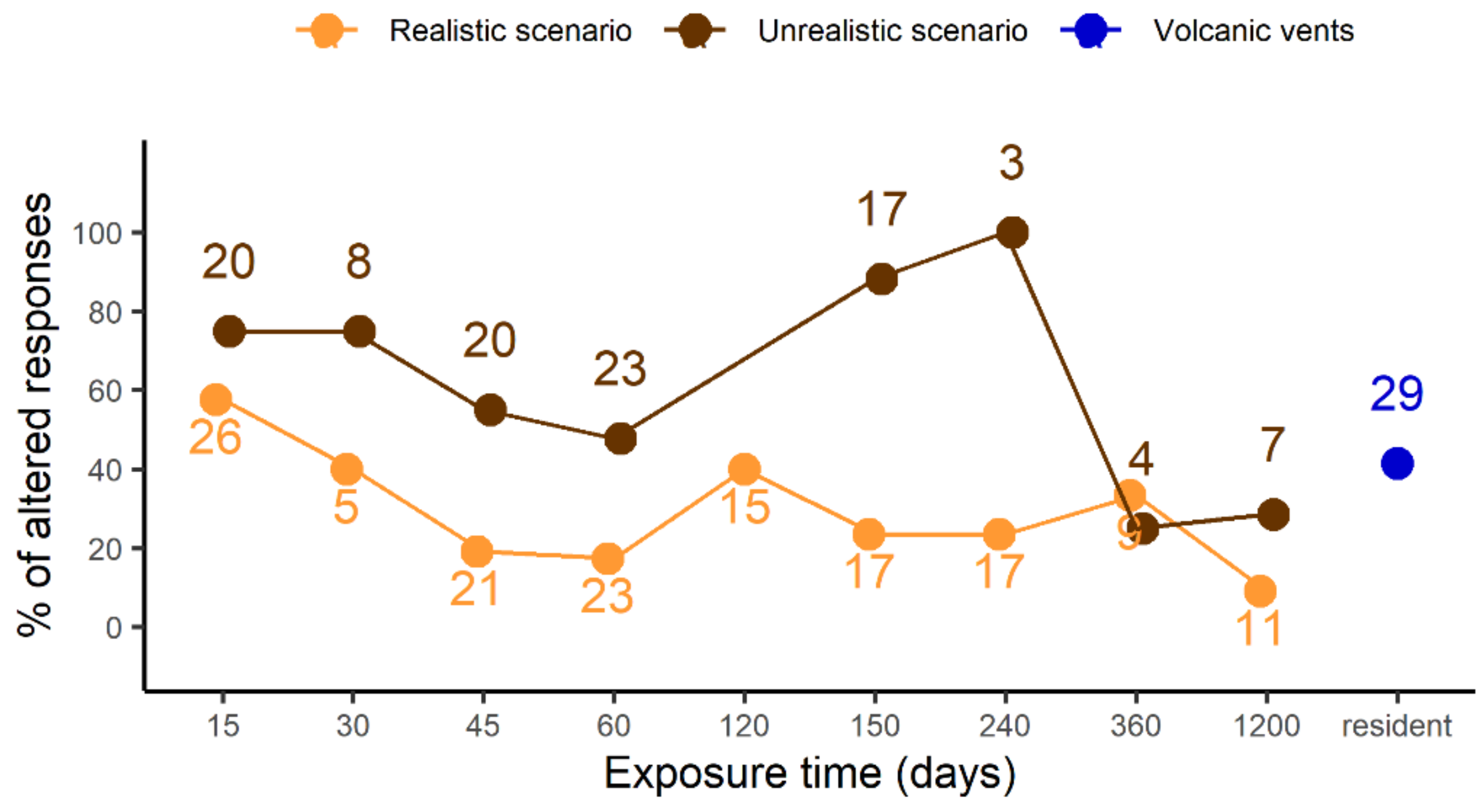
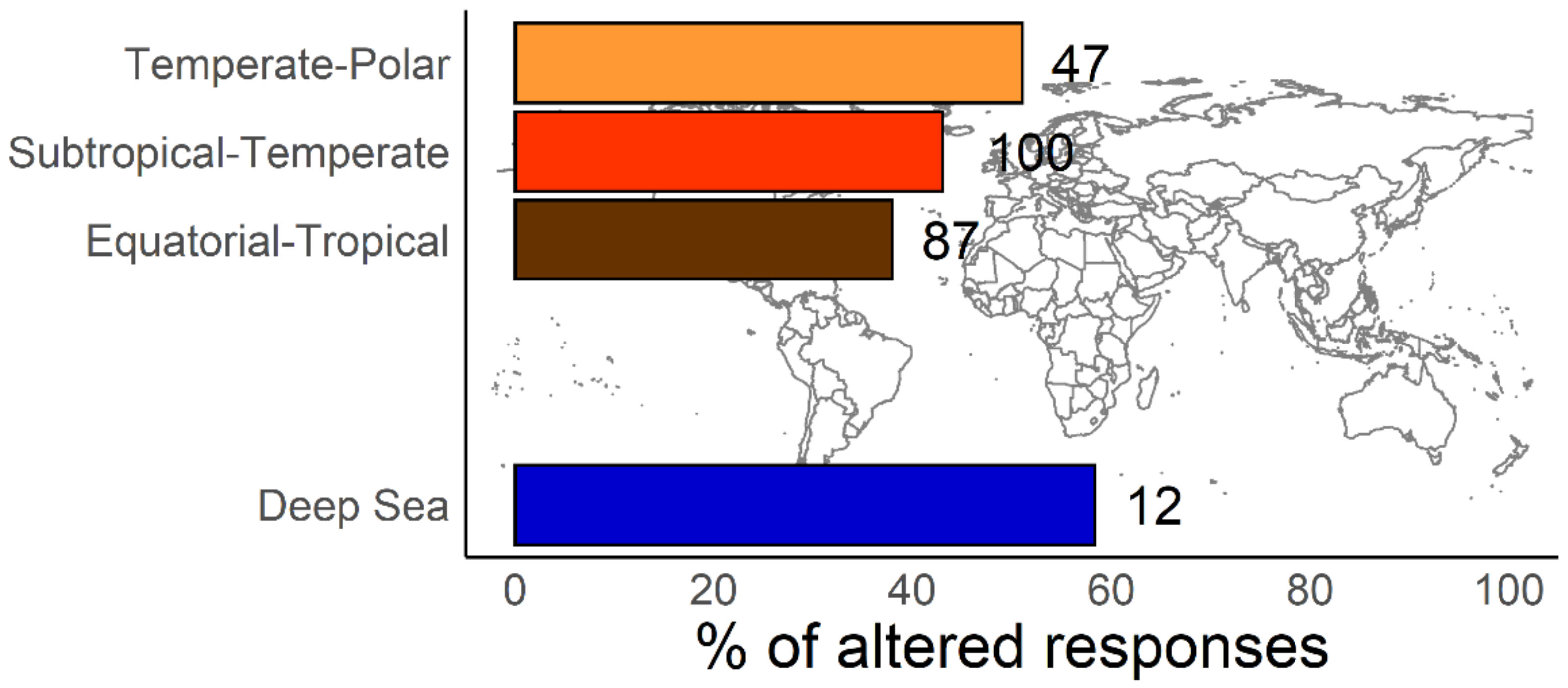
6. Conclusions and Future Perspectives

According to the IPCC RCP8.5 scenario, a decrease of up to 0.4 units in pH (average surface seawater total scale pH 7.7) is expected by 2100. Data collected in this review suggest that the adult life stage of echinoids is robust against SWA when the pH reduction is smaller than 0.4 units. This is also in accordance with previous findings regarding other echinoderms [128]. However, the among-species differences in susceptibility to SWA have been highlighted, as summarized in Figure 1. Taking into account the geographical range and the variables considered (calcification, physiology, behaviour, and reproduction), some species (such as S. intermedius and A. crassispina) could be more vulnerable than others. Nonetheless, the responses obtained depend also on the exposure’s duration and the pH scenario used.

To check whether or not differences occurred between realistic and unrealistic exposure scenarios (i.e., ΔpH ≤ 0.4 or >0.4 units, respectively) and whether an influence of the experiment duration was present, a generalized linear model (glm) was performed using a binomial distribution, with RStudio [129]. The whole dataset was considered, including effects on calcification, physiology, behaviour, and reproduction. Research data on CO₂ vent echinoids were excluded. For the analysis, a dummy variable was added in the dataset, assigning 0 if there were no changes compared with the control conditions, or 1 if a statistically significant change was present. A statistically significant influence of the time (Chisq = 24.914, Df = 8, p = 0.002) and the scenario (Chisq = 28.344, Df = 1, p < 0.001) was revealed, but not of the two factors’ interaction (Chisq = 10.018, Df = 7, p = 0.188).

In Figure 2, the percentage of altered responses is reported based on the time of exposure and the realistic or unrealistic scenario used. In general, almost half (43%) of the endpoints were altered by the reduction in pH, and a considerable proportion of the studies revealed SWA alterations even in long-term experiments. As can be seen, echinoids are able to acclimate much faster to a pH reduction of less than 0.4 units (Figure 2).

After 15 days of exposure, animals are able to cope with the physico-chemical changes induced by laboratory exposure. Instead, much more time is needed for animals exposed to ΔpH > 0.4 units. In this case, no signs of recovery are visible after 30 days of exposure (>70% of effects due to SWA). In the experiments that exposed echinoids for a time frame between 45 and 60 days, nearly 50–60% of the endpoints showed changes due to lower pH. Conversely, in the same time frame, the percentage of changes was ~20% if the ΔpH was ≤ 0.4 units. Differences compared with control conditions were also recorded after exposures lasted between 120 and 240 days in scenarios close to IPCC RCP8.5 (ΔpH 0.5 in [61]) or under more severe conditions (ΔpH 0.82 and 1.31 in [39,40]). A sensible decrease in the % of change compared with the control (suggesting the improvement in the adaptation capability of the echinoids) was detected only in experiments lasting one year or more [42,44].

Data from CO₂ vent sea urchins revealed that the percentage of change detected with respect to control sites was 41% (Figure 2).

Studies where the endpoints were analysed multiple times during the exposure highlighted the importance of this approach. For example, P. lividus specimens maintained at ΔpH 0.4 for six months were impacted by SWA at the beginning of the exposure but showed acclimation capability towards the end of the exposure [25]. Repeated measurements over time evidenced the subtle effects of SWA that could go unnoticed using a single-timepoint experiment. To obtain a complete picture of the SWA effects in future studies, the length of the exposure to the experimental pH levels and a repeated-measurements approach need to be considered. This is crucial to provide information of high quality and importance.

Some of the features altered by low pH might be functional for living in future OA conditions. Changes in dissolved inorganic carbon and the alkalinity of coelomic fluid are useful for animals to maintain a stable coelomic pH value [78]. Moreover, the animals resident in vent sites showed alterations compared with animals from control sites [45,58]. For example, P. lividus from a vent system showed enhanced defence capability of its immune cells, with the modulation of several enzymes and proteins involved in their metabolic pathways and increased antioxidant activities. The observed changes, promoting the defensive and homeostatic abilities of the immune system, represented an adaptive response of animals to reduced pH. No alterations in biomineralization, mechanical properties, physiological responses or oxidative damage in tissues were found [52,58]. Therefore, differences in the biological traits of sea urchins living at high pCO₂ for a long time (both in natural and laboratory exposure) are not necessarily an impairment, as they may be functional in terms of the animal well-being, potentially without negative effects on reproduction [51,84,122]. To shed light on and sustain this hypothesis, multigenerational studies are needed, even though they are complex and difficult to complete successfully.

Further studies should also adopt a multigenerational approach in order to assess whether the calcification, physiological performances, behaviour and reproduction of sea urchin adults coping with OA would remain the same in future generations. These experiments could help to answer questions about future community structures and potential positive transgenerational effects also involving tolerance to pollutants, ocean warming, deoxygenation and other environmental stressors. Multigenerational studies take into account that gametes and early life stages are more sensitive than adults to environmental changes and the possible impact on fertilization may have strong effects at the population level [130]. An overpopulation or a depletion of sea urchins is often associated with a shift from a kelp-dominated ecosystem to barrens and vice versa [131,132,133,134,135]. For example, in the Mediterranean basin, variations in the grazing pressure of P. lividus and A. lixula drove changes from a complex community dominated by erect algae to a simpler one dominated by few encrusting algae [136].

Furthermore, a growing number of studies highlights intraspecific and inter-sexual variability in the animals’ responses to SWA [13,25,137,138,139,140,141,142]. This implies that natural populations may be disproportionately affected and some individuals may be preadapted to future OA scenarios. Indeed, oysters of the species Saccostrea glomerata, whose bred lines were selected in an aquaculture facility, were found to be more resilient to OA conditions compared with a wild population [143]. OA may be emphasized in coastal areas by eutrophication and hypoxia [19,144,145], but the animals that inhabit these highly variable environments might have an inherent capacity to tolerate near-future OA scenarios [146,147]. Therefore, future studies should also consider the environmental history experienced by animals, either by pooling animals from different areas to average the results or by carrying out parallel experiments with animals from different areas. Indeed, the natural local variability in seawater chemistry can be crucial in shaping coastal population responses to climate change drivers [24,26,27,148]. In natural environments (particularly in estuarine, coastal and upwelling areas), pH and alkalinity do not have stable values and fluctuate broadly, with daily and seasonal changes and local variability [24,27,61,148]. Since variability in pH values may be present also in future OA scenarios, caging experiments in CO₂ vent systems or laboratory experiments that consider this natural variability in seawater chemistry will be useful to better model future acidification conditions. In this regard, although studies carried out with animals sampled in naturally acidified environments are outnumbered by laboratory experiments, they provide more insights into the potential adaptability of the echinoids and the evolutionary consequences of OA.

Regional range also has an influence, albeit slightly, on the susceptibility of sea urchins to OA. In a previous work, Watson and colleagues [149] compared the growth and calcification of marine invertebrates (among which echinoids) collected from the North Pole to the South Pole and found a latitudinal trend in shell morphology and composition. The authors claimed that, in a climate change scenario, this would differently affect animals and communities at different latitudinal ranges [149]. Although not statistically significant (glm with binomial distribution, excluding deep-sea and CO₂ vent experiments; factor “latitudinal range” Chisq = 2.149, Df = 2, p = 0.341), our literature survey confirmed the latitudinal trend observed, since differences in the responses have been found based on the climate region of animals’ collection. In sea urchins, 38% of the endpoints analysed were affected by low pH exposure when the geographical range was between equatorial to tropical regions. For example, sea urchin growth was impaired in S. virgulata exposed at a pH of 7.8 and 7.6 for 14 days [59], but similar results were not obtained in Echinometra sp. [35,42] or in Heliocidaris erythrogramma [34] and growth even increased in sea urchins resident in vent systems at a pH of 7.48 [45]. In the case of sea urchins from subtropical–temperate and temperate–polar areas, 43% and 51%, respectively, of the endpoints analysed were affected by SWA conditions (Figure 3). In this case, growth was reduced in P. lividus [37] and S. droebachiensis [46] exposed to pH 7.7 and 7.4 for 60 and 42 days, respectively. Although genetic and phenotypical differences (e.g., growth and metabolic rates) are obviously present among the variety of species considered, overall observations indicate that animals collected in the equatorial–subtropical areas might be less impacted by SWA than those collected from the subtropical areas to the Poles.

Although some echinoid species are still understudied (Figure 1), the knowledge concerning SWA effects on sea urchins has been growing in the last two decades, opening new questions to be addressed. For example, the majority of the studies in this review were performed using a stable pH value. However, in the environment, physico-chemical variables fluctuate, and it has been demonstrated that the effect of pH is different in the latter condition (e.g., [76,150]). Moreover, long-term multigenerational experiments combining SWA with other stressors will be crucial for studying the effects of climate change on echinoid populations.

Author Contributions

D.A. designed and wrote the present manuscript. M.G.M. contributed to the interpretation of the results available in the literature and supervised the present manuscript. The final version of the manuscript has been approved by all authors. All authors have read and agreed to the published version of the manuscript.

Funding

This research received no external funding.

Institutional Review Board Statement

Not Applicable.

Informed Consent Statement

Not Applicable.

Data Availability Statement

Not Applicable.

Acknowledgments

The authors wish to thank the anonymous reviewers for the constructive suggestions that helped them to improve the quality of the work.

Conflicts of Interest

The authors declare no conflict of interest.

References

Pörtner, H.-O.; Roberts, D.C.; Masson-Delmotte, V.; Zhai, P.; Tignor, M.; Poloczanska, E.; Mintenbeck, K.; Alegría, A.; Nicolai, M.; Okem, A.; et al. (Eds.) IPCC 2019 Special Report on the Ocean and Cryosphere in a Changing Climate; Cambridge University Press: Cambridge, UK; New York, NY, USA, 2019; 755p. [Google Scholar] [CrossRef]
Le Quéré, C.; Raupach, M.R.; Canadell, J.G.; Marland, G.; Bopp, L.; Ciais, P.; Conway, T.J.; Doney, S.C.; Feely, R.A.; Foster, P.; et al. Trends in the sources and sinks of carbon dioxide. Nat. Geosci. 2009, 2, 831–836. [Google Scholar] [CrossRef]
Zeebe, R.E.; Zachos, J.C.; Caldeira, K.; Tyrrell, T. OCEANS: Carbon emissions and acidification. Science 2008, 321, 51–52. [Google Scholar] [CrossRef] [PubMed]
Masson-Delmotte, V.; Zhai, P.; Pörtner, H.-O.; Roberts, D.; Skea, J.; Shukla, P.R.; Pirani, A.; Moufouma-Okia, W.; Péan, C.; Pidcock, R.; et al. (Eds.) IPCC 2018 Summary for Policymakers. In Global Warming of 1.5 °C; An IPCC Special Report on the impacts of global warming of 1.5°C above pre-industrial levels and related global greenhouse gas emission pathways, in the context of strengthening the global response to the threat of climate change, sustainable development, and efforts to eradicate poverty; World Meteorological Organization: Geneva, Switzerland, 2018; 32p., Available online: https://www.ipcc.ch/site/assets/uploads/sites/2/2019/05/SR15_SPM_version_report_LR.pdf (accessed on 23 March 2022).
Doney, S.C.; Fabry, V.J.; Feely, R.A.; Kleypas, J.A. Ocean acidification: The other CO₂ problem. Ann. Rev. Mar. Sci. 2009, 1, 169–192. [Google Scholar] [CrossRef] [PubMed] [Green Version]
Caldeira, K.; Wickett, M.E. Anthropogenic carbon and ocean pH. Nature 2003, 425, 365. [Google Scholar] [CrossRef] [PubMed]
Orr, J.C.; Fabry, V.J.; Aumont, O.; Bopp, L.; Doney, S.C.; Feely, R.A.; Gnanadesikan, A.; Gruber, N.; Ishida, A.; Joos, F.; et al. Anthropogenic ocean acidification over the twenty-first century and its impact on calcifying organisms. Nature 2005, 437, 681–686. [Google Scholar] [CrossRef]
Raven, J.; Caldeira, K.; Elderfield, H.; Hoegh-Guldberg, O.; Liss, P.; Riebesell, U.; Shepherd, J.; Turley, C.; Watson, A. Ocean Acidification Due to Increasing Atmospheric Carbon Dioxide; The Royal Society: London, UK, 2005; ISBN 0-85403-617-2. [Google Scholar]
Hu, M.; Tseng, Y.-C.; Su, Y.-H.; Lein, E.; Lee, H.-G.; Lee, J.-R.; Dupont, S.; Stumpp, M. Variability in larval gut pH regulation defines sensitivity to ocean acidification in six species of the Ambulacraria superphylum. Proc. R. Soc. B Biol. Sci. 2017, 284, 20171066. [Google Scholar] [CrossRef]
Chan, K.Y.K.; Grunbaum, D.; O’Donnell, M.J. Effects of ocean-acidification-induced morphological changes on larval swimming and feeding. J. Exp. Biol. 2011, 214, 3857–3867. [Google Scholar] [CrossRef] [Green Version]
Couturier, C.S.; Stecyk, J.A.W.; Rummer, J.L.; Munday, P.L.; Nilsson, G.E. Species-specific effects of near-future CO₂ on the respiratory performance of two tropical prey fish and their predator. Comp. Biochem. Physiol.-A Mol. Integr. Physiol. 2013, 166, 482–489. [Google Scholar] [CrossRef] [Green Version]
Spady, B.L.; Nay, T.J.; Rummer, J.L.; Munday, P.L.; Watson, S.-A. Aerobic performance of two tropical cephalopod species unaltered by prolonged exposure to projected future carbon dioxide levels. Conserv. Physiol. 2019, 7, coz024. [Google Scholar] [CrossRef]
Range, P.; Chícharo, M.A.; Ben-Hamadou, R.; Piló, D.; Fernandez-Reiriz, M.J.; Labarta, U.; Marin, M.G.; Bressan, M.; Matozzo, V.; Chinellato, A.; et al. Impacts of CO₂-induced seawater acidification on coastal Mediterranean bivalves and interactions with other climatic stressors. Reg. Environ. Chang. 2014, 14, 19–30. [Google Scholar] [CrossRef]
Ries, J.B.; Cohen, A.L.; McCorkle, D.C. Marine calcifiers exhibit mixed responses to CO₂-induced ocean acidification. Geology 2009, 37, 1131–1134. [Google Scholar] [CrossRef]
Wang, M.; Jeong, C.B.; Lee, Y.H.; Lee, J.S. Effects of ocean acidification on copepods. Aquat. Toxicol. 2018, 196, 17–24. [Google Scholar] [CrossRef]
Yamada, Y.; Ikeda, T. Acute toxicity of lowered pH to some oceanic zooplankton. Plankt. Biol. Ecol. 1999, 46, 62–67. [Google Scholar]
McClintock, J.B.; Amsler, M.O.; Angus, R.A.; Challener, R.C.; Schram, J.B.; Amsler, C.D.; Mah, C.L.; Cuce, J.; Baker, B.J. The Mg-calcite composition of Antarctic echinoderms: Important implications for predicting the impacts of ocean acidification. J. Geol. 2011, 119, 457–466. [Google Scholar] [CrossRef]
Dupont, S.; Dorey, N.; Thorndyke, M. What meta-analysis can tell us about vulnerability of marine biodiversity to ocean acidification? Estuar. Coast. Shelf Sci. 2010, 89, 182–185. [Google Scholar] [CrossRef]
Wootton, J.T.; Pfister, C.A.; Forester, J.D. Dynamic patterns and ecological impacts of declining ocean pH in a high-resolution multi-year dataset. Proc. Natl. Acad. Sci. USA 2008, 105, 18848–18853. [Google Scholar] [CrossRef] [Green Version]
Moschino, V.; Marin, M.G. Spermiotoxicity and embryotoxicity of triphenyltin in the sea urchin Paracentrotus lividus Lmk. Appl. Organomet. Chem. 2002, 16, 175–181. [Google Scholar] [CrossRef]
Bellas, J.; Granmo, Å.; Beiras, R. Embryotoxicity of the antifouling biocide zinc pyrithione to sea urchin (Paracentrotus lividus) and mussel (Mytilus edulis). Mar. Pollut. Bull. 2005, 50, 1382–1385. [Google Scholar] [CrossRef]
Bellas, J.; Fernández, N.; Lorenzo, I.; Beiras, R. Integrative assessment of coastal pollution in a Ría coastal system (Galicia, NW Spain): Correspondence between sediment chemistry and toxicity. Chemosphere 2008, 72, 826–835. [Google Scholar] [CrossRef]
Dupont, S.; Ortega-Martínez, O.; Thorndyke, M. Impact of near-future ocean acidification on echinoderms. Ecotoxicology 2010, 19, 449–462. [Google Scholar] [CrossRef]
Vargas, C.A.; Lagos, N.A.; Lardies, M.A.; Duarte, C.; Manríquez, P.H.; Aguilera, V.M.; Broitman, B.; Widdicombe, S.; Dupont, S. Species-specific responses to ocean acidification should account for local adaptation and adaptive plasticity. Nat. Ecol. Evol. 2017, 1, 1–7. [Google Scholar] [CrossRef] [PubMed] [Green Version]
Asnicar, D.; Novoa-Abelleira, A.; Minichino, R.; Badocco, D.; Pastore, P.; Finos, L.; Munari, M.; Marin, M.G. When site matters: Metabolic and behavioural responses of adult sea urchins from different environments during long-term exposure to seawater acidification. Mar. Environ. Res. 2021, 169, 105372. [Google Scholar] [CrossRef] [PubMed]
Aguilera, V.M.; Vargas, C.A.; Lardies, M.A.; Poupin, M.J. Adaptive variability to low-pH river discharges in Acartia tonsa and stress responses to high pCO₂ conditions. Mar. Ecol. 2016, 37, 215–226. [Google Scholar] [CrossRef]
Vargas, C.A.; Cuevas, L.A.; Broitman, B.R.; San Martin, V.A.; Lagos, N.A.; Gaitán-Espitia, J.D.; Dupont, S. Upper environmental pCO₂ drives sensitivity to ocean acidification in marine invertebrates. Nat. Clim. Chang. 2022, 12, 200–207. [Google Scholar] [CrossRef]
Nasuchon, N.; Hirasaka, K.; Yamaguchi, K.; Okada, J.; Ishimatsu, A. Effects of elevated carbon dioxide on contraction force and proteome composition of sea urchin tube feet. Comp. Biochem. Physiol. Part D Genom. Proteom. 2017, 21, 10–16. [Google Scholar] [CrossRef] [Green Version]
Miles, H.; Widdicombe, S.; Spicer, J.I.; Hall-Spencer, J. Effects of anthropogenic seawater acidification on acid-base balance in the sea urchin Psammechinus miliaris. Mar. Pollut. Bull. 2007, 54, 89–96. [Google Scholar] [CrossRef]
Smith, A.M.; Clark, D.E.; Lamare, M.D.; Winter, D.J.; Byrne, M. Risk and resilience: Variations in magnesium in echinoid skeletal calcite. Mar. Ecol. Prog. Ser. 2016, 561, 1–16. [Google Scholar] [CrossRef] [Green Version]
Chave, K.E. Aspects of the Biogeochemistry of Magnesium 1. Calcareous Marine Organisms. J. Geol. 1954, 62, 266–283. [Google Scholar] [CrossRef]
Andersson, A.J.; Mackenzie, F.T.; Bates, N.R. Life on the margin: Implications of ocean acidification on Mg-calcite, high latitude and cold-water marine calcifiers. Mar. Ecol. Prog. Ser. 2008, 373, 265–273. [Google Scholar] [CrossRef]
Lebrato, M.; McClintock, J.B.; Amsler, M.O.; Ries, J.B.; Egilsdottir, H.; Lamare, M.; Amsler, C.D.; Challener, R.C.; Schram, J.B.; Mah, C.L.; et al. From the Arctic to the Antarctic: The major, minor, and trace elemental composition of echinoderm skeletons. Ecology 2013, 94, 1434. [Google Scholar] [CrossRef]
Wolfe, K.; Dworjanyn, S.A.; Byrne, M. Effects of ocean warming and acidification on survival, growth and skeletal development in the early benthic juvenile sea urchin (Heliocidaris erythrogramma). Glob. Chang. Biol. 2013, 19, 2698–2707. [Google Scholar] [CrossRef]
Moulin, L.; Grosjean, P.; Leblud, J.; Batigny, A.; Dubois, P. Impact of elevated pCO₂ on acid–base regulation of the sea urchin Echinometra mathaei and its relation to resistance to ocean acidification: A study in mesocosms. J. Exp. Mar. Bio. Ecol. 2014, 457, 97–104. [Google Scholar] [CrossRef]
Zhan, Y.; Cui, D.; Xing, D.; Zhang, J.; Zhang, W.; Li, Y.; Li, C.; Chang, Y. CO₂-driven ocean acidification repressed the growth of adult sea urchin Strongylocentrotus intermedius by impairing intestine function. Mar. Pollut. Bull. 2020, 153, 110944. [Google Scholar] [CrossRef]
Cohen-Rengifo, M.; Agüera, A.; Bouma, T.; M’Zoudi, S.; Flammang, P.; Dubois, P. Ocean warming and acidification alter the behavioral response to flow of the sea urchin Paracentrotus lividus. Ecol. Evol. 2019, 9, 12128–12143. [Google Scholar] [CrossRef] [Green Version]
Asnaghi, V.; Chindris, A.; Leggieri, F.; Scolamacchia, M.; Brundu, G.; Guala, I.; Loi, B.; Chiantore, M.; Farina, S. Decreased pH impairs sea urchin resistance to predatory fish: A combined laboratory-field study to understand the fate of top-down processes in future oceans. Mar. Environ. Res. 2020, 162, 105194. [Google Scholar] [CrossRef]
Taylor, J.R.; Lovera, C.; Whaling, P.J.; Buck, K.R.; Pane, E.F.; Barry, J.P. Physiological effects of environmental acidification in the deep-sea urchin Strongylocentrotus fragilis. Biogeosciences 2014, 11, 1413–1423. [Google Scholar] [CrossRef] [Green Version]
Wang, G.; Yagi, M.; Yin, R.; Lu, W.; Ishimatsu, A. Effects of elevated seawater CO₂ on feed intake, oxygen consumption and morphology of Aristotle’s lantern in the sea urchin Anthocidaris crassispina. J. Mar. Sci. Technol. 2013, 21, 192–200. [Google Scholar] [CrossRef]
Dworjanyn, S.A.; Byrne, M. Impacts of ocean acidification on sea urchin growth across the juvenile to mature adult life-stage transition is mitigated by warming. Proc. R. Soc. B Biol. Sci. 2018, 285, 20172684. [Google Scholar] [CrossRef] [Green Version]
Moulin, L.; Grosjean, P.; Leblud, J.; Batigny, A.; Collard, M.; Dubois, P. Long-term mesocosms study of the effects of ocean acidification on growth and physiology of the sea urchin Echinometra mathaei. Mar. Environ. Res. 2015, 103, 103–114. [Google Scholar] [CrossRef]
Uthicke, S.; Patel, F.; Karelitz, S.; Luter, H.; Webster, N.; Lamare, M. Key biological responses over two generations of the sea urchin Echinometra sp. A under future ocean conditions. Mar. Ecol. Prog. Ser. 2020, 637, 87–101. [Google Scholar] [CrossRef] [Green Version]
Morley, S.A.; Suckling, C.C.; Clark, M.S.; Cross, E.L.; Peck, L.S. Long-term effects of altered pH and temperature on the feeding energetics of the Antarctic sea urchin, Sterechinus neumayeri. Biodiversity 2016, 17, 34–45. [Google Scholar] [CrossRef] [Green Version]
Uthicke, S.; Ebert, T.; Liddy, M.; Johansson, C.; Fabricius, K.E.; Lamare, M. Echinometra sea urchins acclimatized to elevated pCO₂ at volcanic vents outperform those under present-day pCO₂ conditions. Glob. Chang. Biol. 2016, 22, 2451–2461. [Google Scholar] [CrossRef]
Holtmann, W.C.; Stumpp, M.; Gutowska, M.A.; Syré, S.; Himmerkus, N.; Melzner, F.; Bleich, M. Maintenance of coelomic fluid pH in sea urchins exposed to elevated CO₂: The role of body cavity epithelia and stereom dissolution. Mar. Biol. 2013, 160, 2631–2645. [Google Scholar] [CrossRef]
Calosi, P.; Rastrick, S.P.S.; Graziano, M.; Thomas, S.C.; Baggini, C.; Carter, H.A.; Hall-Spencer, J.M.; Milazzo, M.; Spicer, J.I. Distribution of sea urchins living near shallow water CO₂ vents is dependent upon species acid–base and ion-regulatory abilities. Mar. Pollut. Bull. 2013, 73, 470–484. [Google Scholar] [CrossRef] [PubMed] [Green Version]
Johnson, R.; Harianto, J.; Thomson, M.; Byrne, M. The effects of long-term exposure to low pH on the skeletal microstructure of the sea urchin Heliocidaris erythrogramma. J. Exp. Mar. Bio. Ecol. 2020, 523, 151250. [Google Scholar] [CrossRef]
Dery, A.; Collard, M.; Dubois, P. Ocean Acidification Reduces Spine Mechanical Strength in Euechinoid but Not in Cidaroid Sea Urchins. Environ. Sci. Technol. 2017, 51, 3640–3648. [Google Scholar] [CrossRef] [PubMed]
Bray, L.; Pancucci-Papadopulou, M.A.; Hall-Spencer, J.M. Sea urchin response to rising pCO₂ shows ocean acidification may fundamentally alter the chemistry of marine skeletons. Mediterr. Mar. Sci. 2014, 15, 510–519. [Google Scholar] [CrossRef] [Green Version]
Hazan, Y.; Wangensteen, O.S.; Fine, M. Tough as a rock-boring urchin: Adult Echinometra sp. EE from the Red Sea show high resistance to ocean acidification over long-term exposures. Mar. Biol. 2014, 161, 2531–2545. [Google Scholar] [CrossRef]
Di Giglio, S.; Spatafora, D.; Milazzo, M.; M’Zoudi, S.; Zito, F.; Dubois, P.; Costa, C. Are control of extracellular acid-base balance and regulation of skeleton genes linked to resistance to ocean acidification in adult sea urchins? Sci. Total Environ. 2020, 720, 137443. [Google Scholar] [CrossRef]
Asnaghi, V.; Collard, M.; Mangialajo, L.; Gattuso, J.P.; Dubois, P. Bottom-up effects on biomechanical properties of the skeletal plates of the sea urchin Paracentrotus lividus (Lamarck, 1816) in an acidified ocean scenario. Mar. Environ. Res. 2019, 144, 56–61. [Google Scholar] [CrossRef] [Green Version]
Byrne, M.; Smith, A.M.; West, S.; Collard, M.; Dubois, P.; Graba-landry, A.; Dworjanyn, S.A. Warming Influences Mg2+ Content, While Warming and Acidification Influence Calcification and Test Strength of a Sea Urchin. Environ. Sci. Technol. 2014, 48, 12620–12627. [Google Scholar] [CrossRef]
Collard, M.; Rastrick, S.P.S.; Calosi, P.; Demolder, Y.; Dille, J.; Findlay, H.S.; Hall-Spencer, J.M.; Milazzo, M.; Moulin, L.; Widdicombe, S.; et al. The impact of ocean acidification and warming on the skeletal mechanical properties of the sea urchin Paracentrotus lividus from laboratory and field observations. ICES J. Mar. Sci. 2016, 73, 727–738. [Google Scholar] [CrossRef] [Green Version]
Di Giglio, S.; Agüera, A.; Pernet, P.; M’Zoudi, S.; Angulo-Preckler, C.; Avila, C.; Dubois, P. Effects of ocean acidification on acid-base physiology, skeleton properties, and metal contamination in two echinoderms from vent sites in Deception Island, Antarctica. Sci. Total Environ. 2021, 765, 142669. [Google Scholar] [CrossRef]
Uthicke, S.; Liddy, M.; Nguyen, H.D.; Byrne, M. Interactive effects of near-future temperature increase and ocean acidification on physiology and gonad development in adult Pacific sea urchin, Echinometra sp. A. Coral Reefs 2014, 33, 831–845. [Google Scholar] [CrossRef] [Green Version]
Migliaccio, O.; Pinsino, A.; Maffioli, E.; Smith, A.M.; Agnisola, C.; Matranga, V.; Nonnis, S.; Tedeschi, G.; Byrne, M.; Gambi, M.C.; et al. Living in future ocean acidification, physiological adaptive responses of the immune system of sea urchins resident at a CO₂ vent system. Sci. Total Environ. 2019, 672, 938–950. [Google Scholar] [CrossRef]
Anand, M.; Rangesh, K.; Maruthupandy, M.; Jayanthi, G.; Rajeswari, B.; Priya, R.J. Effect of CO₂ driven ocean acidification on calcification, physiology and ovarian cells of tropical sea urchin Salmacis virgulata—A microcosm approach. Heliyon 2021, 7, e05970. [Google Scholar] [CrossRef]
Emerson, C.E.; Reinardy, H.C.; Bates, N.R.; Bodnar, A.G. Ocean acidification impacts spine integrity but not regenerative capacity of spines and tube feet in adult sea urchins. R. Soc. Open Sci. 2017, 4, 170140. [Google Scholar] [CrossRef] [Green Version]
Shetye, S.S.; Naik, H.; Kurian, S.; Shenoy, D.; Kuniyil, N.; Fernandes, M.; Hussain, A. pH variability off Goa (eastern Arabian Sea) and the response of sea urchin to ocean acidification scenarios. Mar. Ecol. 2020, 41, 1–11. [Google Scholar] [CrossRef]
Mos, B.; Byrne, M.; Dworjanyn, S.A. Biogenic acidification reduces sea urchin gonad growth and increases susceptibility of aquaculture to ocean acidification. Mar. Environ. Res. 2016, 113, 39–48. [Google Scholar] [CrossRef] [Green Version]
Wood, H.L.; Spicer, J.I.; Widdicombe, S. Ocean acidification may increase calcification rates, but at a cost. Proc. R. Soc. B Biol. Sci. 2008, 275, 1767–1773. [Google Scholar] [CrossRef] [Green Version]
Long, W.C.; Swiney, K.M.; Foy, R.J. Effects of ocean acidification on the embryos and larvae of red king crab, Paralithodes camtschaticus. Mar. Pollut. Bull. 2013, 69, 38–47. [Google Scholar] [CrossRef] [PubMed]
Melzner, F.; Gutowska, M.A.; Langenbuch, M.; Dupont, S.; Lucassen, M.; Thorndyke, M.C.; Bleich, M.; Pörtner, H.O. Physiological basis for high CO₂ tolerance in marine ectothermic animals: Pre-adaptation through lifestyle and ontogeny? Biogeosciences 2009, 6, 2313–2331. [Google Scholar] [CrossRef] [Green Version]
Kaniewska, P.; Campbell, P.R.; Kline, D.I.; Rodriguez-Lanetty, M.; Miller, D.J.; Dove, S.; Hoegh-Guldberg, O. Major cellular and physiological impacts of ocean acidification on a reef building coral. PLoS ONE 2012, 7, e34659. [Google Scholar] [CrossRef] [PubMed] [Green Version]
Heuer, R.M.; Grosell, M. Physiological impacts of elevated carbon dioxide and ocean acidification on fish. Am. J. Physiol. Integr. Comp. Physiol. 2014, 307, R1061–R1084. [Google Scholar] [CrossRef] [PubMed] [Green Version]
Pörtner, H. Ecosystem effects of ocean acidification in times of ocean warming: A physiologist’s view. Mar. Ecol. Prog. Ser. 2008, 373, 203–217. [Google Scholar] [CrossRef] [Green Version]
Pörtner, H.O.; Bock, C.; Reipschläger, A. Modulation of the cost of pHi regulation during metabolic depression: A 31P-NMR study in invertebrate (Sipunculus nudus) isolated muscle. J. Exp. Biol. 2000, 203, 2417–2428. [Google Scholar] [CrossRef]
Reipschläger, A.; Pörtner, H.O. Metabolic depression during environmental stress: The role of extracellular versus intracellular pH in Sipunculus nudus. J. Exp. Biol. 1996, 199, 1801–1807. [Google Scholar] [CrossRef]
Langenbuch, M.; Bock, C.; Leibfritz, D.; Pörtner, H.O. Effects of environmental hypercapnia on animal physiology: A 13C NMR study of protein synthesis rates in the marine invertebrate Sipunculus nudus. Comp. Biochem. Physiol. Part A Mol. Integr. Physiol. 2006, 144, 479–484. [Google Scholar] [CrossRef] [Green Version]
Carey, N.; Harianto, J.; Byrne, M. Sea urchins in a high-CO₂ world: Partitioned effects of body size, ocean warming and acidification on metabolic rate. J. Exp. Biol. 2016, 219, 1178–1186. [Google Scholar] [CrossRef] [Green Version]
Brockington, S.; Peck, L. Seasonality of respiration and ammonium excretion in the Antarctic echinoid Sterechinus neumayeri. Mar. Ecol. Prog. Ser. 2001, 219, 159–168. [Google Scholar] [CrossRef] [Green Version]
Catarino, A.I.; Bauwens, M.; Dubois, P. Acid-base balance and metabolic response of the sea urchin Paracentrotus lividus to different seawater pH and temperatures. Environ. Sci. Pollut. Res. 2012, 19, 2344–2353. [Google Scholar] [CrossRef]
Stumpp, M.; Trübenbach, K.; Brennecke, D.; Hu, M.Y.; Melzner, F. Resource allocation and extracellular acid-base status in the sea urchin Strongylocentrotus droebachiensis in response to CO₂ induced seawater acidification. Aquat. Toxicol. 2012, 110–111, 194–207. [Google Scholar] [CrossRef]
Small, D.P.; Milazzo, M.; Bertolini, C.; Graham, H.; Hauton, C.; Hall-Spencer, J.M.; Rastrick, S.P.S. Temporal fluctuations in seawater pCO₂ may be as important as mean differences when determining physiological sensitivity in natural systems. ICES J. Mar. Sci. 2016, 73, 604–612. [Google Scholar] [CrossRef] [Green Version]
Lewis, C.; Ellis, R.P.; Vernon, E.; Elliot, K.; Newbatt, S.; Wilson, R.W. Ocean acidification increases copper toxicity differentially in two key marine invertebrates with distinct acid-base responses. Sci. Rep. 2016, 6, 1–10. [Google Scholar] [CrossRef] [Green Version]
Collard, M.; Dery, A.; Dehairs, F.; Dubois, P. Euechinoidea and Cidaroidea respond differently to ocean acidification. Comp. Biochem. Physiol.-Part A Mol. Integr. Physiol. 2014, 174, 45–55. [Google Scholar] [CrossRef]
Marčeta, T.; Matozzo, V.; Alban, S.; Badocco, D.; Pastore, P.; Marin, M.G. Do males and females respond differently to ocean acidification? An experimental study with the sea urchin Paracentrotus lividus. Environ. Sci. Pollut. Res. 2020, 27, 39516–39530. [Google Scholar] [CrossRef]
Harianto, J.; Aldridge, J.; Torres Gabarda, S.A.; Grainger, R.J.; Byrne, M. Impacts of Acclimation in Warm-Low pH Conditions on the Physiology of the Sea Urchin Heliocidaris erythrogramma and Carryover Effects for Juvenile Offspring. Front. Mar. Sci. 2021, 7, 1–18. [Google Scholar] [CrossRef]
Spicer, J.I.; Widdicombe, S.; Needham, H.R.; Berge, J.A. Impact of CO₂-acidified seawater on the extracellular acid-base balance of the northern sea urchin Strongylocentrotus dröebachiensis. J. Exp. Mar. Bio. Ecol. 2011, 407, 19–25. [Google Scholar] [CrossRef]
Leite Figueiredo, D.A.; Branco, P.C.; dos Santos, D.A.; Emerenciano, A.K.; Iunes, R.S.; Shimada Borges, J.C.; Machado Cunha da Silva, J.R. Ocean acidification affects parameters of immune response and extracellular pH in tropical sea urchins Lytechinus variegatus and Echinometra luccunter. Aquat. Toxicol. 2016, 180, 84–94. [Google Scholar] [CrossRef]
Dupont, S.; Thorndyke, M. Relationship between CO₂-driven changes in extracellular acid-base balance and cellular immune response in two polar echinoderm species. J. Exp. Mar. Bio. Ecol. 2012, 424–425, 32–37. [Google Scholar] [CrossRef]
Kurihara, H.; Yin, R.; Nishihara, G.N.G.; Soyano, K.; Ishimatsu, A. Effect of ocean acidification on growth, gonad development and physiology of the sea urchin Hemicentrotus pulcherrimus. Aquat. Biol. 2013, 18, 281–292. [Google Scholar] [CrossRef] [Green Version]
Rich, W.A.; Schubert, N.; Schläpfer, N.; Carvalho, V.F.; Horta, A.C.L.; Horta, P.A. Physiological and biochemical responses of a coralline alga and a sea urchin to climate change: Implications for herbivory. Mar. Environ. Res. 2018, 142, 100–107. [Google Scholar] [CrossRef]
Burnham, K.A.; Nowicki, R.J.; Hall, E.R.; Pi, J.; Page, H.N. Effects of ocean acidification on the performance and interaction of fleshy macroalgae and a grazing sea urchin. J. Exp. Mar. Bio. Ecol. 2022, 547, 151662. [Google Scholar] [CrossRef]
Sun, T.; Tang, X.; Jiang, Y.; Wang, Y. Seawater acidification induced immune function changes of haemocytes in Mytilus edulis: A comparative study of CO₂ and HCl enrichment. Sci. Rep. 2017, 7, 1–10. [Google Scholar] [CrossRef] [PubMed]
Lawrence, J.M.; Lane, J.M. The utilization of nutrients by post-metamorphic echinoderms. In Echinoderm Nutrition; Jangoux, M., Lawrence, J.M., Eds.; CRC Press: London, UK, 2020; pp. 331–371. [Google Scholar]
Shick, J.M. Respiratory Gas Exchange in Echinoderms. In Echinoderm Studies; Jangoux, M., Lawrence, J.M., Eds.; CRC Press: Boca Raton, FL, USA, 2020; pp. 67–110. [Google Scholar]
Cattano, C.; Claudet, J.; Domenici, P.; Milazzo, M. Living in a high CO₂ world: A global meta-analysis shows multiple trait-mediated fish responses to ocean acidification. Ecol. Monogr. 2018, 88, 320–335. [Google Scholar] [CrossRef]
Havenhand, J.N.; Buttler, F.-R.; Thorndyke, M.C.; Williamson, J.E. Near-future levels of ocean acidification reduce fertilization success in a sea urchin. Curr. Biol. 2008, 18, R651–R652. [Google Scholar] [CrossRef] [PubMed] [Green Version]
Beniash, E.; Ivanina, A.; Lieb, N.S.; Kurochkin, I.; Sokolova, I.M. Elevated level of carbon dioxide affects metabolism and shell formation in oysters Crassostrea virginica. Mar. Ecol. Prog. Ser. 2010, 419, 95–108. [Google Scholar] [CrossRef]
Mayzaud, P. Respiration and nitrogen excretion of zooplankton. II. Studies of the metabolic characteristics of starved animals. Mar. Biol. 1973, 21, 19–28. [Google Scholar] [CrossRef]
Bayne, B.L.; Widdows, J.; Thompson, T.J. Physiological integrations. In Marine Mussels: Their Ecology and Physiology; Cambridge University Press: Cambridge, UK, 1976; pp. 121–206. [Google Scholar]
Bayne, B.L.; Brown, D.A.; Burns, K.; Dixon, D.R.; Ivanovici, A.; Livingstone, D.R.; Lowe, D.M.; Moore, M.N.; Stebbing, A.R.D.; Widdows, J. The Effects of Stress and Pollution on Marine Animals; Praeger: Westport, CT, USA, 1985; ISBN 0030570190. [Google Scholar]
Clements, J.C.; Hunt, H.L. Marine animal behaviour in a high CO₂ ocean. Mar. Ecol. Prog. Ser. 2015, 536, 259–279. [Google Scholar] [CrossRef]
Clements, J.C.; Poirier, L.A.; Pérez, F.F.; Comeau, L.A.; Babarro, J.M.F. Behavioural responses to predators in Mediterranean mussels (Mytilus galloprovincialis) are unaffected by elevated pCO₂. Mar. Environ. Res. 2020, 161, 105148. [Google Scholar] [CrossRef]
Clements, J.C.; Darrow, E.S. Eating in an acidifying ocean: A quantitative review of elevated CO₂ effects on the feeding rates of calcifying marine invertebrates. Hydrobiologia 2018, 820, 1–21. [Google Scholar] [CrossRef]
Watson, S.A.; Lefevre, S.; McCormick, M.I.; Domenici, P.; Nilsson, G.E.; Munday, P.L. Marine mollusc predator-escape behaviour altered by near-future carbon dioxide levels. Proc. R. Soc. B Biol. Sci. 2013, 281. [Google Scholar] [CrossRef]
Nilsson, G.E.; Dixson, D.L.; Domenici, P.; McCormick, M.I.; Sørensen, C.; Watson, S.-A.; Munday, P.L. Near-future carbon dioxide levels alter fish behaviour by interfering with neurotransmitter function. Nat. Clim. Chang. 2012, 2, 201–204. [Google Scholar] [CrossRef]
Clements, J.C.; Sundin, J.; Clark, T.D.; Jutfelt, F. Meta-analysis reveals an extreme “decline effect” in the impacts of ocean acidification on fish behavior. PLoS Biol. 2022, 20, e3001511. [Google Scholar] [CrossRef]
Barry, J.P.; Lovera, C.; Buck, K.R.; Peltzer, E.T.; Taylor, J.R.; Walz, P.; Whaling, P.J.; Brewer, P.G. Use of a free ocean CO₂ enrichment (FOCE) system to evaluate the effects of ocean acidification on the foraging behavior of a deep-sea urchin. Environ. Sci. Technol. 2014, 48, 9890–9897. [Google Scholar] [CrossRef] [Green Version]
Persons, M.H.; Walker, S.E.; Rypstra, A.L.; Marshall, S.D. Wolf spider predator avoidance tactics and survival in the presence of diet-associated predator cues (Araneae: Lycosidae). Anim. Behav. 2001, 61, 43–51. [Google Scholar] [CrossRef] [Green Version]
Weis, J.S.; Smith, G.; Zhou, T.; Santiago-Bass, C.; Weis, P. Effects of contaminants on behavior: Biochemical mechanisms and ecological consequences. Bioscience 2001, 51, 209–217. [Google Scholar] [CrossRef] [Green Version]
Zhao, C.; Bao, Z.; Chang, Y. Fitness-related consequences shed light on the mechanisms of covering and sheltering behaviors in the sea urchin Glyptocidaris crenularis. Mar. Ecol. 2016, 37, 998–1007. [Google Scholar] [CrossRef]
Borell, E.M.; Steinke, M.; Fine, M. Direct and indirect effects of high pCO₂ on algal grazing by coral reef herbivores from the Gulf of Aqaba (Red Sea). Coral Reefs 2013, 32, 937–947. [Google Scholar] [CrossRef]
Campbell, J.E.; Craft, J.D.; Muehllehner, N.; Langdon, C.; Paul, V.J. Responses of calcifying algae (Halimeda spp.) to ocean acidification: Implications for herbivores. Mar. Ecol. Prog. Ser. 2014, 514, 43–56. [Google Scholar] [CrossRef]
Percy, J.A. Thermal adaptation in the boreo-arctic echinoid Strongylocentrotus droebachiensis (Müller, 1776). II. Seasonal acclimatization and urchin activity. Physiol. Zool. 1973, 46, 129–138. [Google Scholar] [CrossRef]
Bayed, A.; Quiniou, F.; Benrha, A.; Guillou, M. The Paracentrotus lividus populations from the northern Moroccan Atlantic coast: Growth, reproduction and health condition. J. Mar. Biol. Assoc. UK 2005, 85, 999–1007. [Google Scholar] [CrossRef] [Green Version]
Lawrence, J.M.; Cowell, B.C. The righting response as an indication of stress in Stichaster striatus (Echinodermata, asteroidea). Mar. Freshw. Behav. Physiol. 1996, 27, 239–248. [Google Scholar] [CrossRef]
Verling, E.; Crook, A.C.; Barnes, D.K.A. Covering behaviour in Paracentrotus lividus: Is light important? Mar. Biol. 2002, 140, 391–396. [Google Scholar] [CrossRef]
Boudouresque, C.F.; Verlaque, M. Paracentrotus lividus. In Sea Urchins: Biology and Ecology; Lawrence, J.M., Ed.; Elsevier B.V.: Amsterdam, The Netherlands, 2020; pp. 447–485. [Google Scholar]
Brothers, C.J.; McClintock, J.B. The effects of climate-induced elevated seawater temperature on the covering behavior, righting response, and Aristotle’s lantern reflex of the sea urchin Lytechinus variegatus. J. Exp. Mar. Bio. Ecol. 2015, 467, 33–38. [Google Scholar] [CrossRef]
Pinna, S.; Pais, A.; Campus, P.; Sechi, N.; Ceccherelli, G. Habitat preferences of the sea urchin Paracentrotus lividus. Mar. Ecol. Prog. Ser. 2012, 445, 173–180. [Google Scholar] [CrossRef] [Green Version]
Dumont, C.P.; Drolet, D.; Deschênes, I.; Himmelman, J.H. Multiple factors explain the covering behaviour in the green sea urchin, Strongylocentrotus droebachiensis. Anim. Behav. 2007, 73, 979–986. [Google Scholar] [CrossRef]
Farina, S.; Tomas, F.; Prado, P.; Romero, J.; Alcoverro, T. Seagrass meadow structure alters interactions between the sea urchin Paracentrotus lividus and its predators. Mar. Ecol. Prog. Ser. 2009, 377, 131–137. [Google Scholar] [CrossRef]
Ziegenhorn, M.A. Sea urchin covering behavior: A comparative review. In Sea Urchin—From Environment to Aquaculture and Biomedicine; InTech: London, UK, 2017. [Google Scholar]
Richner, H.; Milinski, M. On the functional significance of masking behaviour in sea urchins—An experiment with Paracentrotus lividus. Mar. Ecol. Prog. Ser. 2000, 205, 307–308. [Google Scholar] [CrossRef]
Zhao, C.; Ding, J.; Yang, M.; Shi, D.; Yin, D.; Hu, F.; Sun, J.; Chi, X.; Zhang, L.; Chang, Y. Transcriptomes reveal genes involved in covering and sheltering behaviors of the sea urchin Strongylocentrotus intermedius exposed to UV-B radiation. Ecotoxicol. Environ. Saf. 2019, 167, 236–241. [Google Scholar] [CrossRef]
Zhang, L.; Zhang, L.; Shi, D.; Wei, J.; Chang, Y.; Zhao, C. Effects of long-term elevated temperature on covering, sheltering and righting behaviors of the sea urchin Strongylocentrotus intermedius. PeerJ 2017, 5, e3122. [Google Scholar] [CrossRef] [Green Version]
Chi, X.; Sun, J.; Yu, Y.; Luo, J.; Zhao, B.; Han, F.; Chang, Y.; Zhao, C. Fitness benefits and costs of shelters to the sea urchin Glyptocidaris crenularis. PeerJ 2020, 8, e8886. [Google Scholar] [CrossRef] [Green Version]
Dupont, S.; Dorey, N.; Stumpp, M.; Melzner, F.; Thorndyke, M. Long-term and trans-life-cycle effects of exposure to ocean acidification in the green sea urchin Strongylocentrotus droebachiensis. Mar. Biol. 2013, 160, 1835–1843. [Google Scholar] [CrossRef] [Green Version]
Dell’Acqua, O.; Ferrando, S.; Chiantore, M.; Asnaghi, V. The impact of ocean acidification on the gonads of three key Antarctic benthic macroinvertebrates. Aquat. Toxicol. 2019, 210, 19–29. [Google Scholar] [CrossRef]
Kroeker, K.J.; Kordas, R.L.; Crim, R.N.; Singh, G.G. Meta-analysis reveals negative yet variable effects of ocean acidification on marine organisms. Ecol. Lett. 2010, 13, 1419–1434. [Google Scholar] [CrossRef]
Birkhead, T.; Møller, A. Sperm Competition and Sexual Selection; Academic Press Inc.: New York, NY, USA, 1998. [Google Scholar]
Parker, G.A. Sperm competition and its evolutionary consequences in the insects. Biol. Rev. 1970, 45, 525–567. [Google Scholar] [CrossRef]
Gallo, A.; Boni, R.; Tosti, E. Gamete quality in a multistressor environment. Environ. Int. 2020, 138, 105627. [Google Scholar] [CrossRef]
Bednaršek, N.; Calosi, P.; Feely, R.A.; Ambrose, R.; Byrne, M.; Chan, K.Y.K.; Dupont, S.; Padilla-Gamiño, J.L.; Spicer, J.I.; Kessouri, F.; et al. Synthesis of Thresholds of Ocean Acidification Impacts on Echinoderms. Front. Mar. Sci. 2021, 8, 261. [Google Scholar] [CrossRef]
R Core Team. R: A Language and Environment for Statistical Computing; R Foundation for Statistical Computing: Vienna, Austria, 2021. [Google Scholar]
Foo, S.A.; Byrne, M. Marine gametes in a changing ocean: Impacts of climate change stressors on fecundity and the egg. Mar. Environ. Res. 2017, 128, 12–24. [Google Scholar] [CrossRef]
Dijkstra, J.A.; Harris, L.G.; Mello, K.; Litterer, A.; Wells, C.; Ware, C. Invasive seaweeds transform habitat structure and increase biodiversity of associated species. J. Ecol. 2017, 105, 1668–1678. [Google Scholar] [CrossRef] [Green Version]
Fagerli, C.; Norderhaug, K.; Christie, H. Lack of sea urchin settlement may explain kelp forest recovery in overgrazed areas in Norway. Mar. Ecol. Prog. Ser. 2013, 488, 119–132. [Google Scholar] [CrossRef] [Green Version]
Cardona, L.; Moranta, J.; Reñones, O.; Hereu, B. Pulses of phytoplanktonic productivity may enhance sea urchin abundance and induce state shifts in Mediterranean rocky reefs. Estuar. Coast. Shelf Sci. 2013, 133, 88–96. [Google Scholar] [CrossRef]
Hereu, B.; Zabala, M.; Sala, E. Multiple controls of community structure and dynamics in a sublittoral marine environment. Ecology 2008, 89, 3423–3435. [Google Scholar] [CrossRef] [PubMed] [Green Version]
Sala, E.; Ballesteros, E.; Dendrinos, P.; Di Franco, A.; Ferretti, F.; Foley, D.; Fraschetti, S.; Friedlander, A.; Garrabou, J.; Güçlüsoy, H.; et al. The structure of Mediterranean rocky reef ecosystems across environmental and human gradients, and conservation implications. PLoS ONE 2012, 7, e32742. [Google Scholar] [CrossRef] [Green Version]
Gianguzza, P.; Visconti, G.; Gianguzza, F.; Vizzini, S.; Sarà, G.; Dupont, S. Temperature modulates the response of the thermophilous sea urchin Arbacia lixula early life stages to CO₂-driven acidification. Mar. Environ. Res. 2014, 93, 70–77. [Google Scholar] [CrossRef]
Shaw, E.C.; Carpenter, R.C.; Lantz, C.A.; Edmunds, P.J. Intraspecific variability in the response to ocean warming and acidification in the scleractinian coral Acropora pulchra. Mar. Biol. 2016, 163, 210. [Google Scholar] [CrossRef]
Kurihara, H.; Takahashi, A.; Reyes-Bermudez, A.; Hidaka, M. Intraspecific variation in the response of the scleractinian coral Acropora digitifera to ocean acidification. Mar. Biol. 2018, 165, 38. [Google Scholar] [CrossRef]
Dupont, S.; Lundve, B.; Thorndyke, M. Near future ocean acidification increases growth rate of the lecithotrophic larvae and juveniles of the sea star Crossaster papposus. J. Exp. Zool. Part B Mol. Dev. Evol. 2010, 314B, 382–389. [Google Scholar] [CrossRef]
Schlegel, P.; Havenhand, J.N.; Gillings, M.R.; Williamson, J.E. Individual variability in reproductive success determines winners and losers under ocean acidification: A case study with sea urchins. PLoS ONE 2012, 7, 1–8. [Google Scholar] [CrossRef] [Green Version]
Duarte, C.; Navarro, J.M.; Acuña, K.; Torres, R.; Manríquez, P.H.; Lardies, M.A.; Vargas, C.A.; Lagos, N.A.; Aguilera, V. Intraspecific variability in the response of the edible mussel Mytilus chilensis (Hupe) to ocean acidification. Estuaries Coasts 2015, 38, 590–598. [Google Scholar] [CrossRef]
Ellis, R.P.; Davison, W.; Queirós, A.M.; Kroeker, K.J.; Calosi, P.; Dupont, S.; Spicer, J.I.; Wilson, R.W.; Widdicombe, S.; Urbina, M.A. Does sex really matter? Explaining intraspecies variation in ocean acidification responses. Biol. Lett. 2017, 13. [Google Scholar] [CrossRef]
Parker, L.M.; Ross, P.M.; O’Connor, W.A. Populations of the Sydney rock oyster, Saccostrea glomerata, vary in response to ocean acidification. Mar. Biol. 2011, 158, 689–697. [Google Scholar] [CrossRef]
Cai, W.-J.; Hu, X.; Huang, W.-J.; Murrell, M.C.; Lehrter, J.C.; Lohrenz, S.E.; Chou, W.-C.; Zhai, W.; Hollibaugh, J.T.; Wang, Y.; et al. Acidification of subsurface coastal waters enhanced by eutrophication. Nat. Geosci. 2011, 4, 766–770. [Google Scholar] [CrossRef]
Melzner, F.; Thomsen, J.; Koeve, W.; Oschlies, A.; Gutowska, M.A.; Bange, H.W.; Hansen, H.P.; Körtzinger, A. Future ocean acidification will be amplified by hypoxia in coastal habitats. Mar. Biol. 2013, 160, 1875–1888. [Google Scholar] [CrossRef]
Salisbury, J.; Green, M.; Hunt, C.; Campbell, J. Coastal acidification by rivers: A threat to shellfish? Eos Trans. Am. Geophys. Union 2008, 89, 513. [Google Scholar] [CrossRef] [Green Version]
Thomsen, J.; Gutowska, M.A.; Saphörster, J.; Heinemann, A.; Trübenbach, K.; Fietzke, J.; Hiebenthal, C.; Eisenhauer, A.; Körtzinger, A.; Wahl, M.; et al. Calcifying invertebrates succeed in a naturally CO₂-rich coastal habitat but are threatened by high levels of future acidification. Biogeosciences 2010, 7, 3879–3891. [Google Scholar] [CrossRef] [Green Version]
Hofmann, G.E.; Evans, T.G.; Kelly, M.W.; Padilla-Gamiño, J.L.; Blanchette, C.A.; Washburn, L.; Chan, F.; McManus, M.A.; Menge, B.A.; Gaylord, B.; et al. Exploring local adaptation and the ocean acidification seascape—Studies in the California Current Large Marine Ecosystem. Biogeosciences 2014, 11, 1053–1064. [Google Scholar] [CrossRef] [Green Version]
Watson, S.; Peck, L.S.; Tyler, P.A.; Southgate, P.C.; Tan, K.S.; Day, R.W.; Morley, S.A. Marine invertebrate skeleton size varies with latitude, temperature and carbonate saturation: Implications for global change and ocean acidification. Glob. Chang. Biol. 2012, 18, 3026–3038. [Google Scholar] [CrossRef]
Foo, S.A.; Koweek, D.A.; Munari, M.; Gambi, M.C.; Byrne, M.; Caldeira, K. Responses of sea urchin larvae to field and laboratory acidification. Sci. Total Environ. 2020, 723, 138003. [Google Scholar] [CrossRef]

Figure 1. Summary of the effects of seawater acidification on echinoids. For each species and variable considered, colour denotes the percentage of papers showing alterations due to the pH reduction. White: 0–10%; yellow: 10–40%; orange: 40–70%; red: 70–100%; grey: no articles on the topic.

Figure 2. Percentage of altered responses compared with control conditions in sea urchins maintained under either realistic or unrealistic 2100 scenarios (IPCC RCP8.5) along time of exposure (not scaled). Close to each dot, the number of endpoints per case is reported.

Figure 3. Percentage of altered responses in sea urchins from different latitudinal ranges and the deep sea. On the right of each bar, the number of endpoints per case is reported.

Publisher’s Note: MDPI stays neutral with regard to jurisdictional claims in published maps and institutional affiliations.

© 2022 by the authors. Licensee MDPI, Basel, Switzerland. This article is an open access article distributed under the terms and conditions of the Creative Commons Attribution (CC BY) license (https://creativecommons.org/licenses/by/4.0/).

Share and Cite

MDPI and ACS Style

Asnicar, D.; Marin, M.G. Effects of Seawater Acidification on Echinoid Adult Stage: A Review. J. Mar. Sci. Eng. 2022, 10, 477. https://doi.org/10.3390/jmse10040477

AMA Style

Asnicar D, Marin MG. Effects of Seawater Acidification on Echinoid Adult Stage: A Review. Journal of Marine Science and Engineering. 2022; 10(4):477. https://doi.org/10.3390/jmse10040477

Chicago/Turabian Style

Asnicar, Davide, and Maria Gabriella Marin. 2022. "Effects of Seawater Acidification on Echinoid Adult Stage: A Review" Journal of Marine Science and Engineering 10, no. 4: 477. https://doi.org/10.3390/jmse10040477

Note that from the first issue of 2016, this journal uses article numbers instead of page numbers. See further details here.

Article Menu

Effects of Seawater Acidification on Echinoid Adult Stage: A Review

Abstract

1. Introduction

2. SWA Effects on Echinoid Calcification

3. SWA Effects on Echinoid Physiology

4. SWA Effects on Echinoid Behaviour

5. SWA Effects on Echinoid Reproduction

6. Conclusions and Future Perspectives

Author Contributions

Funding

Institutional Review Board Statement

Informed Consent Statement

Data Availability Statement

Acknowledgments

Conflicts of Interest

References

Share and Cite

Article Metrics

Article Access Statistics

Further Information

Guidelines

MDPI Initiatives

Follow MDPI