Dynamical Sliding Mode Control for Robust Dynamic Positioning Systems of FPSO Vessels

Abstract

The conventional proportional derivative (PD) control algorithm with appropriate gain scheduling is generally applied to a dynamic positioning (DP) system. However, finding appropriate gains through gain scheduling makes the DP system more complicated. A sliding-mode control algorithm controls an arbitrary point, such as the turret system on a floating production storage and offloading (FPSO) vessel. This algorithm was developed for DP and can be applied to FPSO vessels considering the uncertainty of the vessel dynamics, unknown time-varying environmental disturbances, and transient performance. To control an arbitrary point on the FPSO vessel using a DP controller, the Jacobian matrix in the kinematic equation is modified to present the arbitrary point in the control. The Lyapunov stability theory is applied in the design of the SM control algorithm to provide robustness to the control system. A time-domain simulation tool was developed to verify the effectiveness of the proposed SM control algorithm. The performance of the control algorithm was evaluated numerically to address its efficacy. The results were compared with those obtained using the conventional PD control algorithm.

1. Introduction

Recently, the demand for advanced marine mechatronics systems has been increasing with the current situation where the region of human production activities is expanding to the deep ocean and polar regions. The dynamic positioning (DP) system is the representative marine mechatronics system. This system adjusts the positions and forces of a number of propulsion systems installed in the hulls and operates along a set route during vessel navigation. Vessels equipped with DP systems are operated in the offshore oil and gas industry because they have economic advantages when compared with traditional methods for maintaining the location of floating structures such as mooring systems or jacket structures. Specifically, DP systems have been applied in marine drilling, dredging, lifting, pipelaying, subsea installation and maintenance, and for transportation of workers between marine structures. These systems have become a major part of the marine industry [1,2,3,4].

The optimal performance of the control system is essential for the effective operation of DP systems used for various purposes in the ocean. When the DP system was first developed in the early 1960s, a single-input single-output (SISO) proportional-integral-differential (PID) controller with a low-pass filter [5] was applied to independently control the surge, sway, and yaw motions of vessels. Balchen et al. [6] and Grimble et al. [7] applied multi-variable optimal control and Kalman filter to DP systems, which enabled reliability and stability of such systems to be used in a wide range of areas. Based on the nonlinear control theory, Lee et al. [8], Fossen et al. [1] and Kim et al. [9] developed weathervaning control to automatically set the heading angle to the direction of the wave loads acting on the ship to reduce fuel consumption and CO₂ emissions. Kim et al. [10] demonstrated the possibility of using weathervaning control applied to the process of loading and offloading for floating production storage and offloading (FPSO) with tandem arrangement and shuttle tanker. Sørensen [11] introduced DP control techniques for the application of marine mechatronics systems. Yu et al. [12] applied the $H_{\infty }$ control technique to DP control and compared its performance with linear-quadratic-Gaussian control (LQG) through numerical simulations. Lee et al. [13] applied the theory of linear quadratic regulator (LQR) and LQR with an error integrator (LQI). Kim et al. [14] also developed a PID controller that included an anti-windup controller that restrained the propensity of divergence of the integral controller in the DP system of a shuttle tanker. Jeon et al. [15] studied the gain scheduling of the PID controller using a fuzzy system. Aleksander et al. [16] presented a dynamic positioning scheme based on a model-predictive control algorithm that combines positioning control and thrust allocation to theoretically yield a near-optimal controller output. Borkowski [17] suggested designing an expert system that includes a function to automatically stabilize ship’s course with the inference engine. Additionally, Peng et al. [18] introduced a cooperative control scheme for the dynamic positioning of multiple offshore vessels based on a dynamic surface control technique with the input-to-state stability of a closed-loop network system.

Robust DP control techniques applicable to a variety of vessels and work scenarios are essential because of the recent demands in marine operations with respect to increasing types and frequencies. DP systems are based on conventional controllers; proportional derivative (PD) controller is a widely used linear controller. Conventional PD controllers typically use gain scheduling based on each characteristic of marine operation scenarios and ocean environmental changes to ensure DP performance. However, there are some problems related to the application of a linear PD controller to the DP system. Gain scheduling should be adjusted for each vessel model and ocean environment while operating the DP system. If the gain values are not appropriate in a specific vessel model and ocean environment, the conventional PD controller sometimes results in control difficulty with unsatisfactory performance in nonlinear plant controls, especially in FPSO vessels with turret mooring systems.

A sliding mode (SM) controller was applied to the DP system to overcome the limitation of the conventional linear controller. The SM controller approach enables the realization of control performance and stability requirements for the desired position. Because the SM controller uses vessel model information, an estimated mass is used as a parameter. Furthermore, the same performance is ensured for different loading conditions without requiring a gain-scheduling approach, and the SM controller can be easily adjusted with simple equations. Therefore, the SM controller can be applied in a wide range of environmental conditions without performance degradation. Tannuri et al. [19,20] applied an SM controller to the application of the motion control of the turret-moored offshore platform along the direction of the horizontal plane, such as surge, sway, and yaw. Kim et al. [21] also applied an SM controller to the depth adjustment and maneuverability control of an unmanned submarine and demonstrated its effectiveness using simulation. Liang et al. [22] presented a finite-time observer-based adaptive sliding mode output feedback control for the DP of ships considering input saturation, unmeasured states, and unknown environment disturbances. Zhao et al. [23] proposed a robust adaptive terminal sliding mode controller for the DP of a semi-submersible offshore platform using a state feedback controller and a robust adaptive terminal sliding mode compensator. Chen et al. [24] developed a novel iterative sliding mode-based output feedback controller for the DP of a ship subjected to ocean environmental disturbance with finite-time state observer. Agostinho et al. [25] proposed the application of a controller with sliding mode control technique to the DP of a floating vessel using numerical simulations and experimental validations.

In this study, a DP system based on the SM controller was developed for the application of FPSO carrying out turret connection work in the sea. The FPSO is equipped with six azimuth thrusters and a turret placed at the bow position of the vessel to carry out access work. A kinematic model is constructed that transforms the center of motion of the vessels because the motion of the vessel should be controlled around the turret installation point located in the bow position. The SM controller, a nonlinear control technique, is used to control the DP system to ensure control performance by selecting control parameters intuitively considering the response characteristics of vessels. In addition, a MATLAB/Simulink-based simulator, which can quantitatively simulate the motion of vessels, was used to evaluate the validity of the proposed control algorithms. The SM controller was designed by applying the Lyapunov stability theory to ensure the robustness of the controller. The effectiveness of the designed SM controllers was evaluated using time-domain simulations and compared with the results of a typical proportional-derivative (PD) controller.

Section 2 describes the configuration of simulators for the performance evaluation of the DP system and the theory of vessel motion utilized therein. Section 3 presents the design of the SM controllers that enables DP control around specific vessel locations. Section 4 presents the results of the DP control simulation in marine environment conditions and Section 5 summarizes the study and presents the conclusions.

2. Methodologies for the DP Control Application

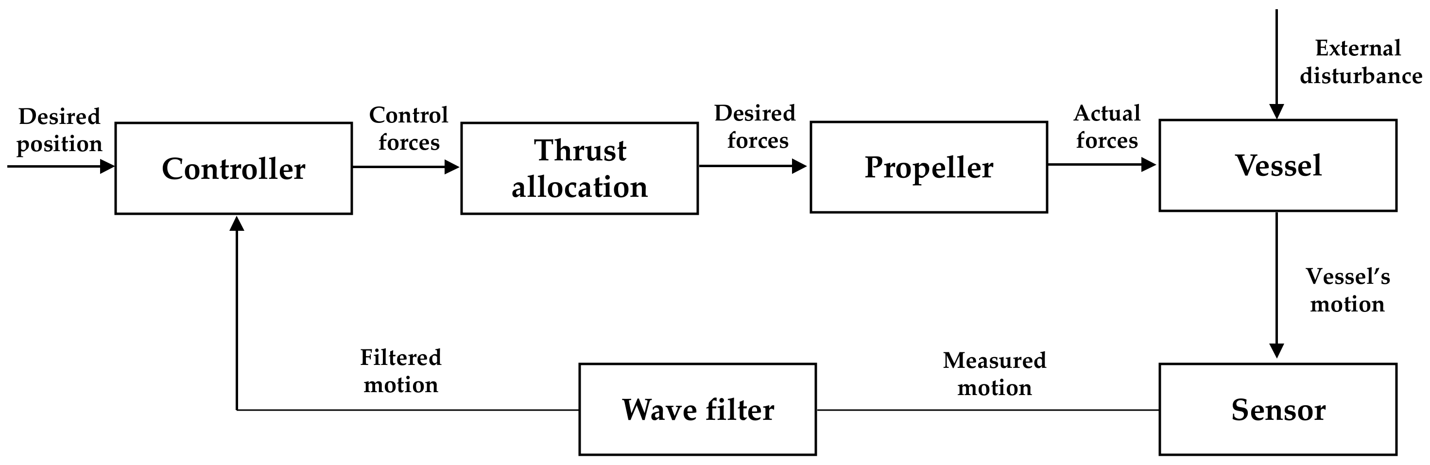
This section describes the methodologies for the DP system. The DP system consists of sensors, controllers and filtering algorithms, and propellers. The sensors are used to measure the positions and angles of the vessel, while the control and thrust allocation algorithms compute the desired forces to be delivered by each propeller to counteract environmental loads such as wind, waves, and current. Figure 1 shows a block diagram of a DP system illustrating the connections between the controller, thruster allocation algorithm, propeller, vessel, sensors and wave filter. A wave filter suppresses the high-frequency motion from the measurements, and a thrust allocation algorithm distributes the desired forces to the propellers equipped in the vessel. To evaluate the motion and control response of vessels equipped with DP systems, a vessel operation simulator with three degrees of freedom (DOF) motions including surge, sway, and yaw was developed based on MATLAB/Simulink.

This section describes a mathematical model that calculates the motion response of a marine surface vessel, considering the effects of sea loads such as from waves, currents, and wind loads. Vessels operating in the sea engage in six DOF motions, which include translational motions such as surge, sway, heave, and rotational motions including roll, pitch, and yaw. Specifically, the DP system in this study considers three DOF horizontal plain models, namely surge, sway, and yaw.

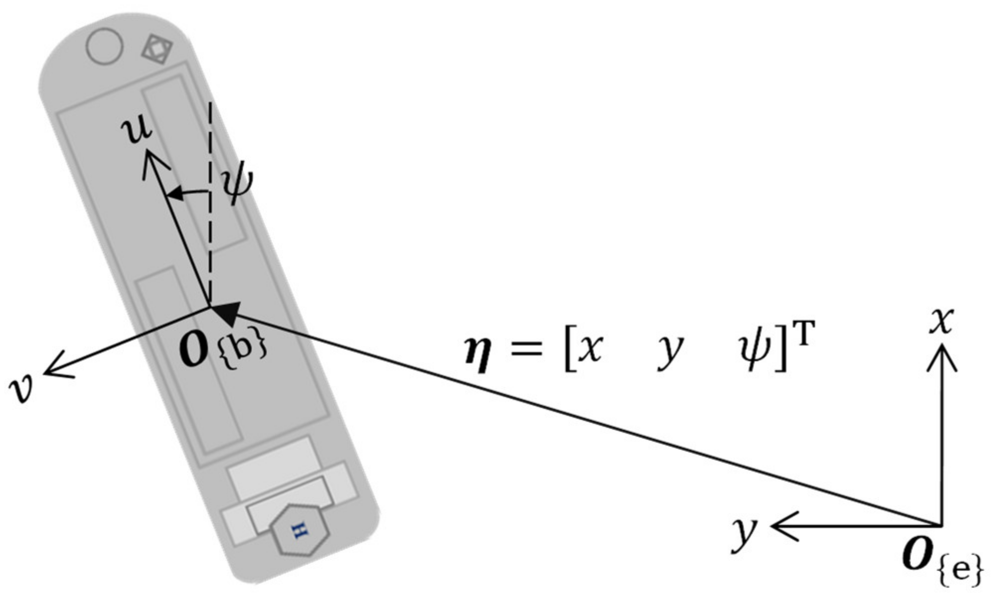
Equation (1) describes the surface vessel motion with a state variable vector representing the position (x, y) and angle (ψ) of the vessel, as defined in the global reference frame {e} shown in Figure 2. The vessel motion consists of a low-frequency motion ${\mathit{\eta }}_L$, which is caused by the effects of wave drift force, current force, wind force, etc., and a high-frequency motion ${\mathit{\eta }}_H$, which is caused by the wave exiting force as follows:

$$\begin{gathered} \mathit{\eta }={\mathit{\eta }}_L+{\mathit{\eta }}_H, \\ {\mathit{\eta }}_L={\left[x_L, y_L, {\psi }_L\right]}^T \mathrm{and} {\mathit{\eta }}_H={\left[x_H, y_H, {\psi }_H\right]}^T. \end{gathered}$$

(1)

Equations (2) and (3) describe the 3 DOF equations of the motion of the vessel and represent the kinematic transformation between the global reference frame and the body-fixed coordinate system for numerical simulations as follows:

$$\begin{gathered} {\dot{\mathit{\eta }}}_L=\mathit{R}\left({\psi }_L\right)\mathbf{\nu }, \\ \mathrm{where}, \mathbf{\nu }={\left[\begin{array}{ccc}u& v& r\end{array}\right]}^T, \mathit{R}\left({\psi }_L\right)=\left[\begin{array}{ccc}\cos {\psi }_L& -\sin {\psi }_L& 0\\ \sin {\psi }_L& \cos {\psi }_L& 0\\ 0& 0& 1\end{array}\right], \end{gathered}$$

(2)

$${\mathit{M}}_{rb}\dot{\mathbf{\nu }}+{\mathit{C}}_{rb}\left(\mathbf{\nu }\right)\mathbf{\nu }+{\mathit{M}}_a{\dot{\mathbf{\nu }}}_{\mathit{r}}+{\mathit{C}}_a\left({\mathbf{\nu }}_{\mathit{r}}\right){\mathbf{\nu }}_{\mathit{r}}+{\mathit{D}}_0\mathbf{\nu }+\mathit{d}\mathit{N}\mathit{L}\left({\mathbf{\nu }}_{\mathit{r}}\right)={\mathit{\tau }}_{wind}+{\mathit{\tau }}_{wave}+\mathit{\tau },$$

(3)

where ν is the velocity vector of the vessel defined in the fixed coordinate system such as the velocity of the surge, sway, and yaw directions. $\mathit{R}\left({\psi }_L\right)$ is the Euler angle transformation matrix that converts the velocity of the body coordinate system into the velocity of the global reference coordinate system.

In Equation (3), ${\mathit{M}}_{rb}$ is the rigid body mass matrix, and ${\mathit{M}}_a$ is the added mass of the fluid around the hull at a low frequency of the vessel. ${\mathit{C}}_{rb}\left(\mathit{\nu }\right)$ and ${\mathit{C}}_a$ are the matrices that express the Coriolis and centripetal forces, respectively, expressing the effect of the hull mass and added mass. Furthermore, ${\mathbf{\nu }}_r$ is the relative velocity defined by ${\mathbf{\nu }}_r=\mathbf{\nu }-{\mathbf{\nu }}_c$, and ${\mathbf{\nu }}_c$ is the current velocity. ${\mathit{D}}_0$ is a linear damping coefficient matrix at low frequencies, characterized by ${\mathit{D}}_0>0$. $\mathit{d}\mathit{N}\mathit{L}\left({\mathbf{\nu }}_r\right)$ is a nonlinear damping force vector that includes the current force and cross-flow damping force. ${\mathit{\tau }}_{wave}$ and ${\mathit{\tau }}_{wind}$ are the wave and wind loads, respectively, at low frequency; they are external forces of the marine environment. τ is the control force generated through the operation of the controller and the propeller. All parameters of matrices are described in Appendix A.

The vessel exposed above the waterline is subjected to sea wind loads according to its shape, as expressed in Equation (4) below,

$${\mathit{\tau }}_{wind}=\frac{1}{2}{\rho }_a{U}_w^2\left[\begin{array}{c}{A}_{fw}{C}_{Xw}\left({\gamma }_w\right)\\ A_{sw}{C}_{Yw}\left({\gamma }_w\right)\\ A_{sw}L{C}_{Nw}\left({\gamma }_w\right)\end{array}\right],$$

(4)

$${\mathit{\tau }}_{wind}={\displaystyle \sum }_{j=1}^N{\displaystyle \sum }_{k=1}^N{A}_j{A}_k\left(QT{F}_R^i\left({\omega }_j, {\omega }_k,{\psi }_L\right)\cos \left({\omega }_{d}t+{ϵ}_d\right)+QT{F}_I^i\left({\omega }_j, {\omega }_k,{\psi }_L\right)\sin \left({\omega }_{d}t+{ϵ}_d\right)\right),$$

(5)

where ${\rho }_a$ is the air density and $U_w$ is the sea wind speed. $A_{fw}$ and $A_{sw}$ are the projection areas along the surge and sway directions of the vessel, respectively. $C_{Xw}$, $C_{Yw}$, and $C_{Nw}$ represent the wind force coefficients in the surge, sway, and yaw directions, respectively. ${\gamma }_w$ is the incident angle of sea wind.

The wave drift force acting on the vessel is described by the quadratic transfer function (QTF) in Equation (5). $A_j$ and $A_k$ refer to the amplitude of the j^th and k^th wave frequencies in the components of the N wave frequencies, which are calculated when generating the irregular wave from the given wave spectrum. The nonlinear transfer function is a function of complex numbers representing the wave drift force calculated through a numerical analysis program using the high-order boundary element method. $QT{F}_R^i$ and $QT{F}_I^i$ represent the real and imaginary parts of the quadratic transfer function, respectively [26]. ${\omega }_j$ and ${\omega }_k$ are the j^th and k^th wave frequencies, respectively. ${\omega }_d$ and ${ϵ}_d$ are the differences of wave frequencies and phases defined by ${\omega }_d={\omega }_i-{\omega }_k$ and ${ϵ}_d={ϵ}_i-{ϵ}_k$, respectivley. Finally, $t$ denotes the time when the ocean waves are generated.

The high-frequency (or wave frequency) motion can be expressed by the response amplitude operator (RAO) as shown in Equation (6):

$${\mathit{\eta }}_H^i={\displaystyle \sum }_{k=1}^N{A}_j\left({\mathrm{RAO}}_R^i\left({\omega }_j,{\psi }_L\right)\cos \left({\omega }_{j}t+{ϵ}_j\right)+{\mathrm{RAO}}_I^i\left({\omega }_j,{\psi }_L\right)\sin \left({\omega }_{j}t+{ϵ}_j\right)\right),$$

(6)

where RAO is also expressed as a harmonic function representing the real and imaginary parts of the RAO.

The noise generated using the sensor modules in the simulators for evaluating DP control responses, as shown in Figure 1, using the primary Gauss-Markov process is given as follows:

$${\dot{y}}^i=-\mu y^i+w,$$

(7)

where $y^i$ is the measured physical value, $w$ is the Gaussian white noise, and $\mu$ is the inverse of the time constant that produces a long-term error in the physical measurement sensor. Fossen [27] describes the configuration of the dynamical term.

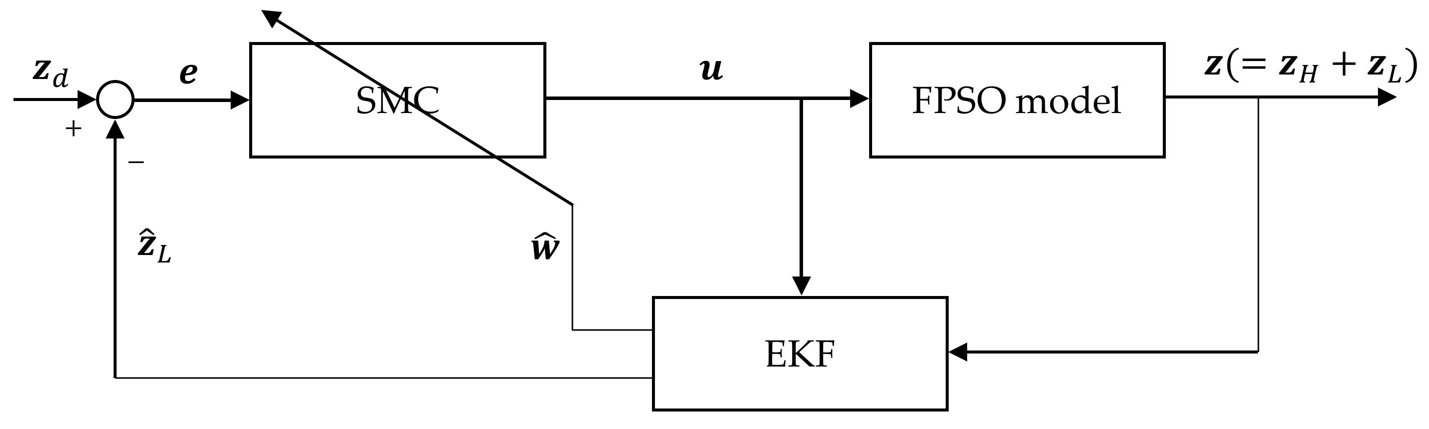
An extended Kalman filter (EKF) is applied to the simulator to separate the low-frequency motion of the vessel model, including the low-frequency motion of the ves-sel, wave frequency, and sensor noise. The estimation algorithm for uncertain external forces was designed in this study by adapting the EKF with a disturbance model of the uncertain external force induced by wave, current, and wind. The EKF is a nonlinear ad-aptation of the Kalman filter, which observes a dynamic system in which zero-mean, Gaussian white noise is assumed in both the dynamics and measurement. The model as a continuous form that is observed by the extended Kalman filter is described by

$$\begin{gathered} \dot{\mathit{x}}\left(t\right)=f\left(\mathit{x}\left(t\right), \mathit{u}\left(t\right)\right)+\mathit{G}\left(t\right)\mathit{w}\left(t\right) \\ \mathit{z}\left(t\right)=h\left(\mathit{x}\left(t\right)\right)+\mathit{v}\left(t\right) \end{gathered}$$

(8)

where $\mathit{x}\left(t\right)$ is the state vector of the system described by $\mathit{x}\left(t\right)={\left[\mathit{\xi }\left(t\right), \dot{\mathit{\xi }}\left(t\right), \mathit{\eta }\left(t\right), \dot{\mathit{\eta }}\left(t\right),F_{ext}\right]}^T$. $\mathit{\xi }\left(t\right)$ is the wave perturbation vector, $\dot{\mathit{\xi }}\left(t\right)$ is the wave frequency vector, $\mathit{\eta }\left(t\right)$ is vessel’s motion vector, $\dot{\mathit{\eta }}\left(t\right)$ is the vessel’s velocity vector, and ${\mathit{F}}_{ext}$ is the uncertain external force vector induced by ocean environmental loads. $\mathit{u}\left(t\right)$ is the input vector described by $\mathit{u}\left(t\right)$ = $\mathit{\tau }$, and $\mathit{z}\left(t\right)$ is the measurement vector measured by motions of the vessel described by $\mathit{z}\left(t\right)$ =${\mathit{\eta }}_m\left(t\right)$. $f$ is the nonlinear state dynamics, $h$ is the nonlinear output function, $\mathit{G}\left(t\right)$ is a vector that describes the noise of each state, and $\mathit{w}\left(t\right)$ and $\mathit{v}\left(t\right)$ are the process and measurement noises, respectively, described by zero-mean Gaussian white noise. The Equation (8) can be transformed into Equation (9) as discretized form with Euler discretization as follows:

$$\begin{gathered} \mathit{x}\left(k\right)=f\left(\mathit{x}\left(k-1\right), \mathit{u}\left(k\right)\right)+\mathit{G}\left(k\right)\mathit{w}\left(k\right) \\ \mathit{z}\left(k\right)=h\left(\mathit{x}\left(k\right)\right)+\mathit{v}\left(k\right). \end{gathered}$$

(9)

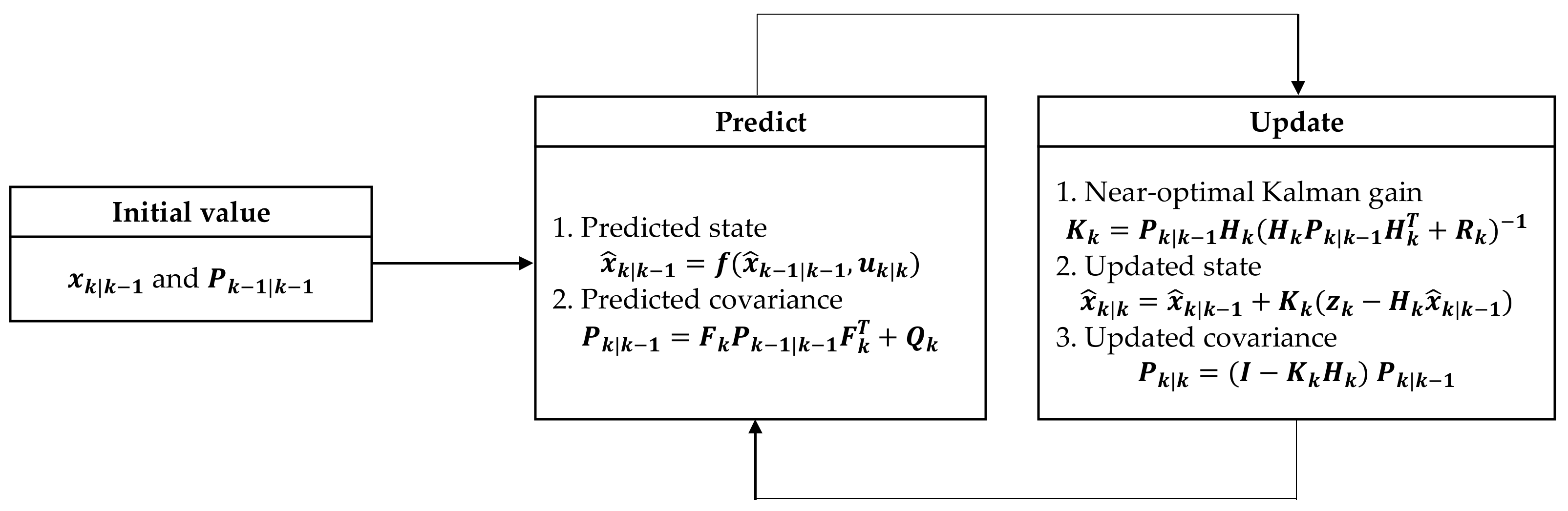
The EKF iterates through the prediction and update steps for each discrete time to estimate the states of the system as shown in Figure 3. The prediction step calculates a predicted state and covariance. The update step calculates the Kalman gain to adjust the covariance of each state and the estimated value based on the difference between the estimated and measured states. Finally, the covariance and state estimates of the next time step can be updated utilizing a Jacobian to linearize the conditions. In this procedure, the algorithm calculates the estimated state vector ${\widehat{\mathit{x}}}_k$ described by ${\widehat{\mathit{x}}}_k={\left[\widehat{\mathit{\xi }}\left(k\right), \dot{\widehat{\mathit{\xi }}}\left(k\right),\widehat{\mathit{\eta }}\left(k\right), \dot{\widehat{\mathit{\eta }}} \left(k\right),{\widehat{\mathit{F}}}_{ext}\left(k\right)\right]}^T$. The EKF calculates estimated external disturbance ${\widehat{\mathit{F}}}_{ext}$ induced by the ocean environment, and it can be applied to the SM controller to compensate the ocean environmental loads. Additionally, ${\mathit{Q}}_k$ and ${\mathit{R}}_k$ are the variance matrices of the process and measurement noises, respectively.

The propulsion system is modeled using a linear differential equation, and the maximum speed rate of each propeller characteristic is limited. In addition, the thrust distribution algorithm that distributes the control forces calculated from the controller to six azimuth propulsion systems is applied based on the Lagrange multiplier theory. Fossen [27] described the details of the extended Kalman filter, propulsion system, and thrust distribution algorithm.

3. Design of a Sliding Mode Controller

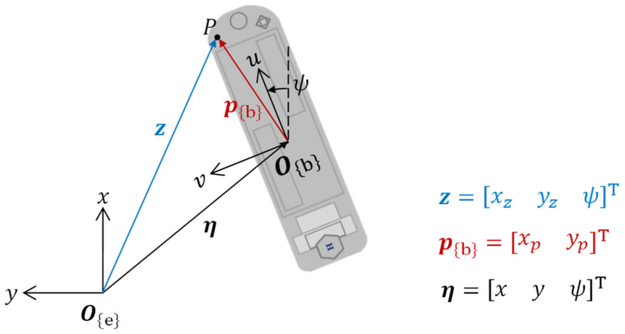
This section describes the design of the sliding mode controller for the dynamic motion control of a vessel model performing turret access operations in the sea. As shown in Figure 4, it is assumed that the turret (${\mathit{p}}_{\left\{b\right\}}$) used to carry out the access work was located at the bow position of the vessel model. Equation (10) describes the kinematic equations for converting the motion of the vessel to ensure that the control algorithm places a specific point z on the target point ${\mathit{z}}_d$. Equation (11) describes the kinematic transformation matrix $\mathit{T}\left(\psi , {\mathit{p}}_{\left\{b\right\}}\right)$ according to the position of the turret ${\mathit{P}}_{\left\{b\right\}}={\left[x_p y_p\right]}^T$ as defined in the body-fixed coordinate system {b}. Additionally, Equation (12) describes the dynamic equation of the motion of the vessel with unknown external forces for the design of the SM controllers. Here are the Equations (10)–(12) as follows:

$$\dot{\mathit{z}}=\mathit{J}\left(\psi , {\mathit{p}}_{\left\{b\right\}}\right)\mathit{\nu }=\mathit{T}\left(\psi , {\mathit{p}}_{\left\{b\right\}}\right)\mathit{R}\left(\psi \right)\mathit{\nu },$$

(10)

$$\mathit{T}\left(\psi , {\mathit{p}}_{\left\{b\right\}}\right)=\left[\begin{array}{lll}1& 0& -x_p\sin \left(\psi \right)-y_p\cos \left(\psi \right)\\ 0& 1& x_p\cos \left(\psi \right)+y_p\sin \left(\psi \right)\\ 0& 0& 1\end{array}\right],$$

(11)

$$\mathit{M}\dot{\mathit{\nu }}=\mathit{u}+\mathit{w},$$

(12)

where $\mathit{M}$ is the mass of a vessel including the low-frequency added mass described by $\mathit{M}={\mathit{M}}_{rb}+{\mathit{M}}_a$, $\mathit{u}$ is the control vector, and $\mathit{w}$ is the uncertainty variable vector including the dynamic model and environmental external force. $\mathit{J}\left(\psi , {\mathit{p}}_{\left\{b\right\}}\right)$ is the transformation matrix that converts the body-fixed coordinate to the global reference coordinate system.

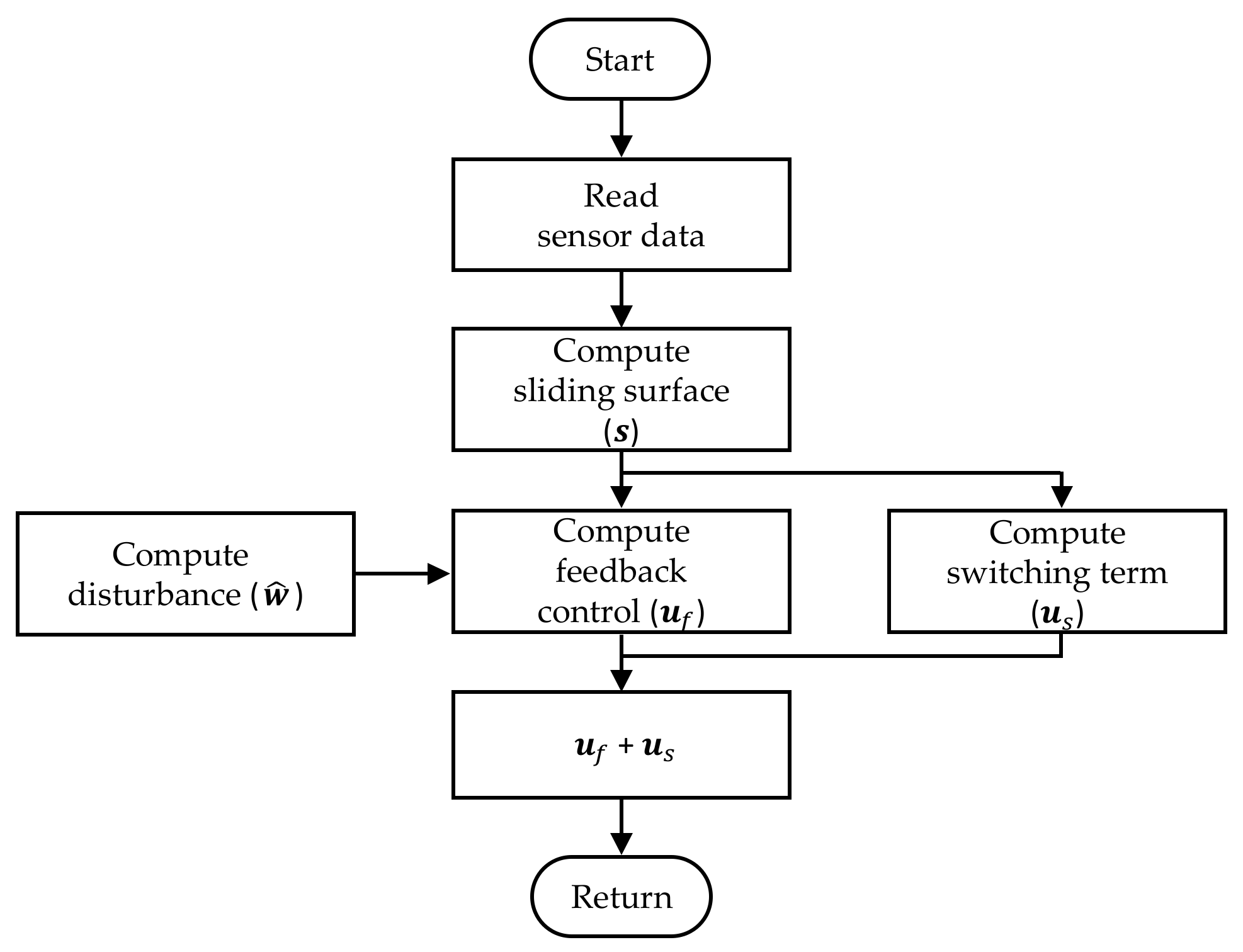
Figure 5 describes the overall procedure of sliding model control. The control objective in this study was to set the turret position at a specific point and to ensure that the velocity of the vessel is zero; this can be expressed by Equation (13) as

$$\mathit{z}\to {\mathit{z}}_d, \mathit{\nu }\to 0 as t\to \infty ,$$

(13)

To achieve this control objective, the system error e can be defined using Equation (14) and the sliding surface for SM control can be defined using Equation (15)

$$\mathit{e}={\mathit{z}}_d-\mathit{z},$$

(14)

$$\mathit{s}=\dot{\mathit{e}}+{\mathit{I}}_{\mathsf{\lambda }}\mathit{e}, {\mathit{I}}_{\mathsf{\lambda }}=\left[\begin{array}{ccc}{\mathsf{\lambda }}_1& 0& 0\\ 0& {\mathsf{\lambda }}_2& 0\\ 0& 0& {\mathsf{\lambda }}_3\end{array}\right]>0$$

(15)

where I_λ is the gain for feedback control when the system state is on a sliding plane, and all elements of I_λ should have positive values. Therefore, the system error e automatically converges to zero when the s = 0 condition is satisfied.

For the design of the robust controller, the Lyapunov function of the control system with the sliding plane variable can be used as shown in Equations (16) and (17), which describes the derivative of the Lyapunov function to determine the stability of the control system.

$$V=\frac{1}{2}{\mathit{s}}^T\mathit{s}>0$$

(16)

$$\dot{V}=s^T\left[-\dot{\mathit{J}}\mathit{\nu }-\mathit{J}{\mathit{M}}^{-1}\left(\mathit{u}+\mathit{w}\right)+{\mathit{I}}_{\mathsf{\lambda }}\dot{\mathit{e}}\right]$$

(17)

The input $\mathit{u}$ of the SM controller consists of the feedback controller ${\mathit{u}}_f$ and the switching controller ${\mathit{u}}_s$. Equation (18) describes the feedback controller ${\mathit{u}}_f$ and Equation (19) describes the relation between the derivative of the Lyapunov function and ${\mathit{u}}_s$. Equation (20) describes the switching controller ${\mathit{u}}_s$. Here are the Equations (18)–(21), as follows:

$${\mathit{u}}_f=\left[-\widehat{\mathit{w}}-\mathit{M}{\mathit{J}}^{-1}\left(\dot{\mathit{J}}\mathit{\upsilon }-{\mathit{I}}_{\mathsf{\lambda }}\dot{\mathit{e}}\right)\right],$$

(18)

$$\dot{V}=s^T\mathit{J}{\mathit{M}}^{-1}\left(\widehat{\mathit{w}}-\mathit{w}\right)-s^T\mathit{J}{\mathit{M}}^{-1}{\mathit{u}}_s,$$

(19)

$$\begin{gathered} {\mathit{u}}_s=\left[F+{\beta }_0\right]\odot \mathrm{sgn}\left(\mathrm{s}\right)\approx \left[F+{\beta }_0\right]\odot \mathrm{sat}\left(\frac{s}{ϵ}\right), \\ F>\left|\widehat{\mathit{w}}-\mathit{w}\right|, {\beta }_0>0, \\ \mathrm{sgn}\left(y\right)=y/\left|y\right|, \mathrm{sat}\left(y\right)=\left\{\begin{array}{cc}y& \left|y\right|\le 1\\ \mathrm{sgn}\left(y\right)& \left|y\right|>1\end{array}\right., \end{gathered}$$

(20)

$$\dot{V}=s^T\mathit{J}{\mathit{M}}^{-1}\left(\widehat{\mathit{w}}-\mathit{w}\right)-s^T\mathit{J}{\mathit{M}}^{-1}\left[F+{\beta }_0\right]\odot \mathrm{sgn}\left(\mathrm{s}\right)<0,$$

(21)

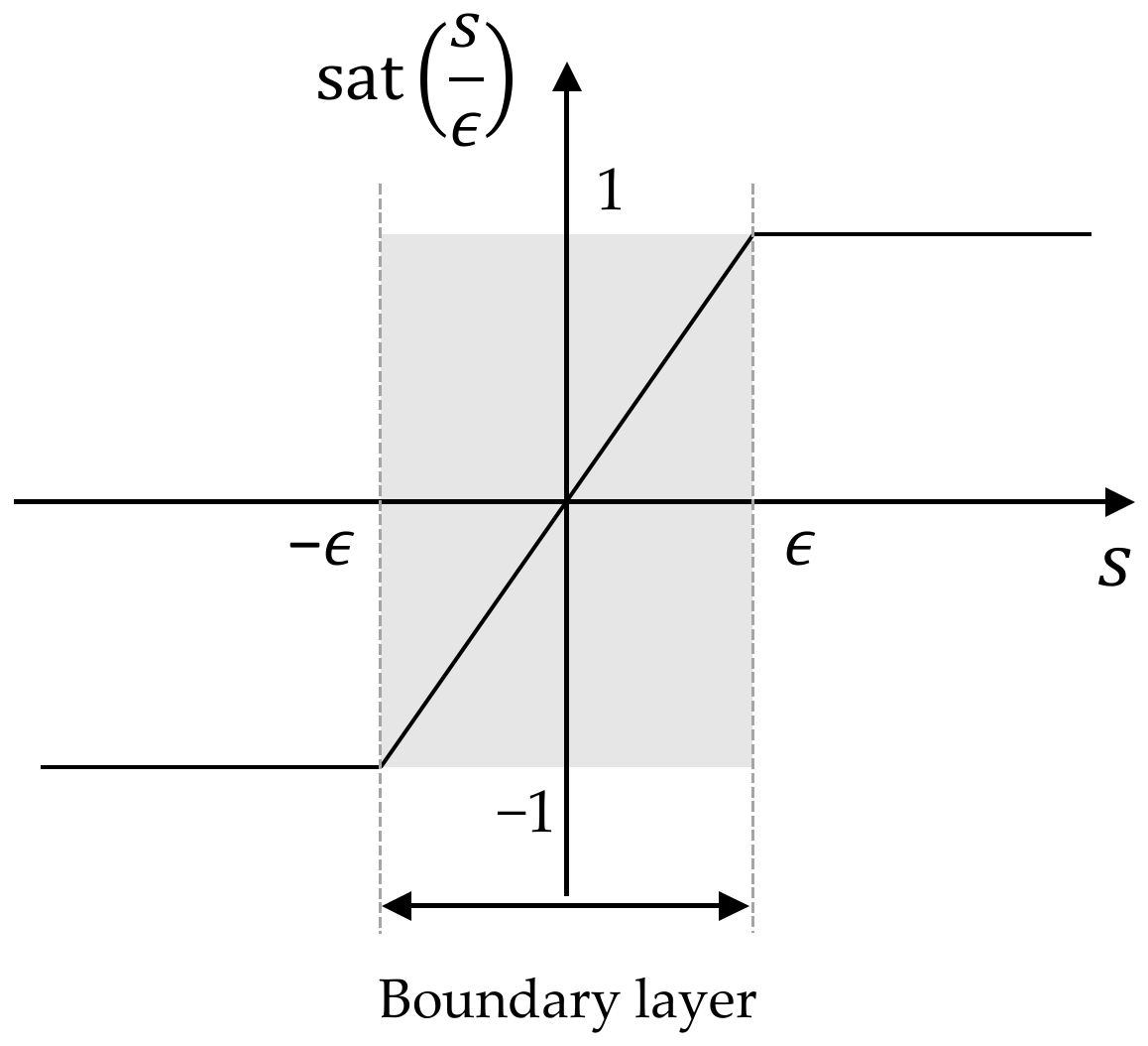
where $\mathit{w}$ is the estimated uncertainty of the external force, ${\beta }_0$ controls the time when the system reaches the sliding plane, and $ϵ$ is a boundary layer that controls the tolerance in the sliding plane, which is the main issue of the sliding mode controller. ⊙ is the vector multiplication operator. In practical applications of sliding mode controllers, the undesirable phenomenon of oscillations called “chattering” having finite frequency and amplitude may occur in the control inputs. Chattering leads to low control accuracy, high wear rate of mechanical systems, and high heat in electrical systems. To reduce the chattering phenomenon, the boundary layer $ϵ$, as shown in Figure 6, is set as smoothing forms of control inputs.

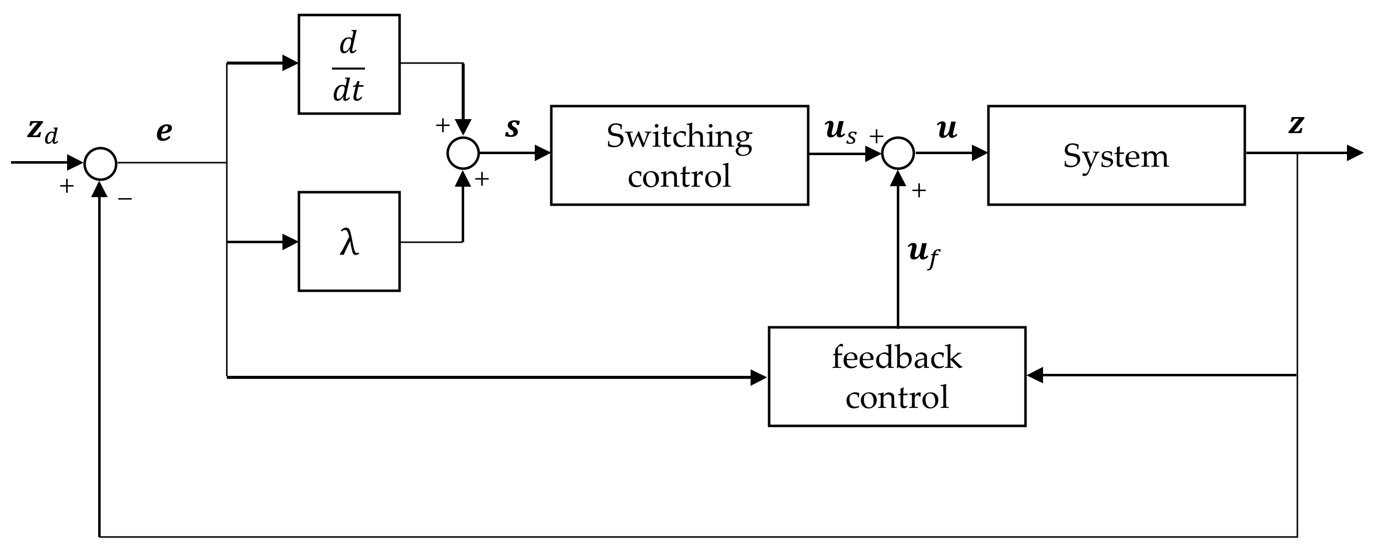
As the system satisfies the condition $\dot{V}<0$ from Equation (21), the system is globally uniformly asymptotically stable according to the LaSalle and Yoshizawa theorem [27,28,29]. Khalil [30,31] described the details of the sliding mode controller. Figure 7 shows the block diagram of the sliding mode controller, illustrating its overall process.

4. Design of a Sliding Mode Controller

This section describes the contents of the DP simulation with the SM controller and their results. It also discusses the characteristics and validity of the SM controllers from the simulation results.

4.1. Configuration of Simulations

Implementing an SM controller requires a dynamic system model, uncertainty estimation, and external forces. In this study, an EKF was used to estimate uncertain external forces and apply them to SM controllers, as illustrated in Figure 8. Figure 9 shows a comparison between actual external disturbance ${\mathit{F}}_{ext}$ and estimated external disturbance ${\widehat{\mathit{F}}}_{ext}$ (blue and red lines, respectively). ${\mathit{F}}_{i, ext}$ (i = 1, 2, and 6) denotes external disturbances along the surge, sway, and yaw directions. The external disturbance error was calculated using Equation (22), and the values were 0.0622, 0.0487, and 0.0453 along the surge, sway, and yaw directions, respectively. The results show that the error is relatively small.

$$error=\frac{\mathrm{rms}\left({\mathit{F}}_{i, ext}-{\widehat{\mathit{F}}}_{i, ext}\right)}{\mathrm{rms}\left({\mathit{F}}_{i, ext}\right)},\left(i=1, 2, 6\right)$$

(22)

It was assumed that the vessel model was built as a FPSO vessel. The FPSO performs turret connection work in the sea, and the SM controller adjusts the position of the turret and validates its performance. The length of the FPSO model was 300 m, and its main specifications and parameters are listed in

Table 1. Vessel Specifications and parameters of FPSO.

Item	Unit	Value
Length (LPP)	m	315
Breadth (B)	m	53
Draft (T)	m	12
Mass	ton	1.950 × 105
Mass moment of inertia (I66)	ton·m2	1.214 × 109
Wind frontal projected area (Afw)	m2	2478
Wind lateral projected area (Asw)	m2	10,863
Added mass in surge (a11)	ton	1.320 × 104
Added mass in sway (a22)	ton	1.058 × 105
Added mass in yaw (a66)	ton·m2	7.132 × 108
Added mass in sway-yaw (a26)	ton·m2	−3.226 × 105

. It was also assumed that six azimuth thrusters with a maximum thrust capacity of 500 kN were installed for DP control of the FPSO, and the information of the thruster is described in

Table 2. Specifications of thruster systems for FPSO.

No.	Type	Location (m)		Max. Thrust (kN)
		X{b}	Y{b}
1	Azimuth	150	0	500
2	Azimuth	130	−17.55	500
3	Azimuth	130	17.55	500
4	Azimuth	−130	−17.55	500
5	Azimuth	−130	17.55	500
6	Azimuth	−130	0	500

.

Table 3. Environmental condition in the simulation.

Environment	Condition
Wave	Hs = 4 m, Tp = 12.5, β = 180°
Wind	Uw = 21 m/s, βw = 170°
Current	Uc = 1.01 m/s, βc = 180°

describes the ocean environmental conditions selected for the simulation.

The control variables for the SM controller include the feedback control gain I_λ, switching control gain F, and sliding plane boundary variable ϵ for chattering reduction. The control variables were set according to

Table 4. Control parameters for the sliding mode control.

Parameter	Value	Setting Variable
Iλ	diag([0.04, 0.04, 0.008]T)
F	[1 × 106, 1 × 106, 1 × 108]T
β0	${\beta }_0=\left|\mathit{s}\right|t_{reach}$	$t_{reach}=30$ s
$ϵ$	$ϵ={\mathit{I}}_{\lambda }\left|{\mathit{e}}_{max}\right|$	${\mathit{e}}_{max}={\left[2, 2, 1\times \left(\pi /180\right)\right]}^T$

, considering the SM control variable proposed by Tannuri et al. [20]. The reaching time t_reach was set to 30 s when the sliding variable was located outside the sliding plane boundary. In addition, the maximum allowable error e_max of surge, sway, and yaw were set as 2 m, 2 m, and 1°, respectively.

4.2. Simulation Results and Discussions

Multiple scenarios were considered for the performance evaluation of the SM controller designed to set the position of the FPSO performing turret access operations as shown in

Table 5. Scenarios for dynamic positioning control of a FPSO.

Scenario	Initial Target	Final Target
Case 1	${\left[120m, 0m, 0°\right]}_{\left\{e\right\}}$	${\left[120m, 0m,-20°\right]}_{\left\{e\right\}}$
Case 2	${\left[120m, 0m, 0°\right]}_{\left\{e\right\}}$	${\left[120m, 0m, 20°\right]}_{\left\{e\right\}}$

. It was assumed in all the scenarios that the turret installed on the FPSO vessel reached the set position to perform the approach operation, initially maintaining the zero target angle (angle on the bow) that the hull holds parallel to the angle of incident waves and currents. Then, the controller changes the target angle. To help understand the control scenario, Figure 10 illustrates the control scenarios for the dynamic positioning of a vessel with environmental disturbance in the clockwise and counter-clockwise DP control. Simulations were conducted to evaluate the effects of different target angles, for 5000 s.

To evaluate the performance of the SM controllers, a proportional-integral (PD) controller was designed with appropriate gains. Then, the performance of the SM controller was compared with that of the PD controller in each control scenario described in Table 5. The PD controller gains used in the simulation are presented in

Table 6. Proportional and derivative gains for comparative simulations.

Gain Type	Value
Proportional	$diag{\left[3.65\times {10}^5, 5.28\times {10}^5, 3.38\times {10}^9\right]}^T$
Derivative	$diag{\left[8.72\times {10}^6, 2.52\times {10}^7, 2.42\times {10}^{11}\right]}^T$

.

Figure 11 shows the simulation results of the dynamic motions of the FPSO vessel and their relative errors concerning surge, sway, and yaw, with a comparison between the SM and PD controllers. The first comparison between the controllers is of clockwise control against external loads to a target angle of −20° in case 1. At the simulation time of 2500 s, a control command was entered to change the target angle from 0 to −20°. The transient region occurs according to this step input. The control output from the SM controller, which rapidly increases in the transition region and then smoothly converges to the control objective is shown in Figure 11a. The SM controller exhibited outstanding performance as the SM controller stabilized the motion of the FPSO vessel in steady-state conditions at approximately 3000 s without overshooting. This means that the SM controller has the ability to eliminate steady-state errors as shown in Figure 11b. By contrast, the result of the PD controller has a different pattern in that it has overshoot, deviations, and offset values and is significantly different from the SM controller. The relative positioning error of the PD controller could not converge to zero and kept outputting deviations and offset values from the control objectives. Figure 11b shows that the PD controller has relatively large errors in comparison with the SM controller.

Figure 12 shows the results of the surge, sway, and yaw motions of the FPSO vessel and their relative errors with the SM and PD controllers according to the case of counter-clockwise control against external loads at a target angle of 20° in case 2. At a simulation time of 2500 s, a control command was entered to change the target angle from 0 to 20°. The variation of motions and relative errors in the PD controller are significant, and the characteristics of the PD controller are clearly evident. The motions of the FPSO vessel and relative errors from the PD controller become unstable and diverse with large oscillations. By contrast, the SM controller can react while maintaining the desired positions and target angles. It seems that the SM controller can effectively eliminate steady-state errors. This is because the SM controller is a multi-input-multi-output (MIMO) system that performs target angle control and simultaneously minimizes interference with other motions such as surge, sway, and yaw. The PD controller is a single-input-single-output (SISO) system that considers all motions as independent control elements. Therefore, the SM controller performs better than the PD controller with ocean environmental disturbances from winds and waves at different target angles.

The control forces and moments along the x, y, and z directions for cases 1 and 2 are shown in Figure 13 to compare the results of the SM and PD controllers. The control force required during the operation of the FPSO turret connection is expressed as the instantaneous control power produced by the controller. In the control forces from the SM controller in case 1, it can be seen that there are no significant variations in the control forces in the results of the SM controller. This means that the SM controller produces a similar control force indicating that less environmental external forces act in the surge when the FPSO controls the target angle against the wave, current, and wind loads. By contrast, there are huge variations in the control forces from 2500 to 2800 s in the transient region from the PD controller in case 1. The system becomes unstable and diverse with a large oscillation in case 2, and the control forces of the PD controller became more necessary.

Regarding the sliding plane, Figure 14 shows the sliding plane response of the SM controller, as defined in Equation (15). s₁, s₂, and s₆ represent the sliding variables in the surge, sway, and yaw directions, respectively, and the dotted line represents the values of the sliding plane boundary variables to mitigate the chattering of the SM controller. The sliding variables in surge and sway motions are located inside the sliding plane boundary at the target angles of −20 and 20° (cases 1 and 2), which means that the sliding plane response is stable. The sliding variable in yaw moves out of the sliding plane boundary when the step input is applied to the system and returns within a certain period (approximately 23 s). The sharp variations appearing on the sliding surface level were due to the abrupt change in the set point. This result indicated that the sliding plane boundary reached time $t_{reach}$ in less than 30 s, as shown in Table 4.

Figure 15 represents the yaw response of the phase plane that simultaneously shows the error $e$ comprising the sliding variable s and the response of the derivative of the error $\dot{e}$ in cases 1 and 2, respectively. The process of convergence to zero is shown as errors, and their derivatives are simultaneously reduced from the results. The blue dotted line represents the sliding boundary variable ϵ for mitigating the chattering of the SM controller. The trajectories in phase planes converged to the sliding surface, and the controller maintained the trajectories inside the boundary layer. These figures indicate that the system is stable because the initial and final sliding variables in the yaw motion are located inside the sliding plane boundaries.

Figure 16 shows the trajectories of the FPSO vessel with DP systems in cases 1 and 2 in comparison with the SM and PD controllers. As shown in Figure 16b, the PD controller could not maintain the angle and position against the wind and wave loads in case 2. These results show that the PD controller is highly sensitive to winds and waves. By contrast, the system output from the SM controller is much more stable, which ensures the robustness of the system to winds and waves, as shown in Figure 16a,b.

Figure 17 and Figure 18 show the root-mean-square (RMS) values of the relative errors of motions and control forces of the FPSO vessel in steady-state conditions between −35 and 25° of the target angles. The RMS values were calculated for the responses to FPSO after steady-state conditions for 30 min. The results show that the PD controller reacts as expected when the target angle is from −20 to 14.2°, but when the target angle is beyond a certain limit above 14.3° and below −20.4°, the RMS values begin substantially increase. With substantially increasing RMS values, the FPSO vessel loses stability and becomes unstable to converge the control objective. By contrast, the RMS values of the errors of motions with the SM controller were close to zero. It is observed that most of the RMS of the vessel motion errors and control forces from the SM controller are generally smaller than the values of the PD controllers. Therefore, satisfactory results were obtained for every target angle between −32 and 20° as shown in Figure 19, in the response of the FPSO with the SM controller. On the other hand, the PD controller can adjust the target angle of the vessel between −20 and 14°. This is another advantage of the SM controller, in addition to its robust characteristic and its applicability in complex marine operations and systems.

5. Concluding Remarks

This paper dealt with a sliding mode control algorithm, which is considered as a robust dynamic positioning control technique applicable to various tasks in the marine industry; its validity was evaluated through a number of simulations. MATLAB/Simulink was used to configure the simulator for the performance evaluation of the DP system with a sliding mode (SM) controller. The simulator consists of a controller module, vessel motion module, sensor module, and filter module. The SM controller was designed to dynamically maintain the turret position by performing the connection work of the FPSO in the ocean. The Lyapunov stability theory was applied at the design stage to ensure the stability of the control system.

Conventional PD controllers were configured and compared to evaluate the validity of the SM-controller-based DP system. SM controllers showed good performance, with only small errors, low required control force, and stability. This is because the SM controller can correct the steady-state error, adjust the control parameters considering the physical characteristics of the vessel, and perform control by considering the interference between surge, sway, and yaw. In particular, the proposed DP system includes a function to adjust the control performance through the selection of control parameters, which intuitively considers the response characteristics of vessels and is highly desirable in diverse and complex marine operations. As an extension of the study, the simulation results from the SM-controller-based DP system should be experimentally validated. In addition, there is scope for future work in updating the proposed DP system with the capabilities to predict incident sea loads from future occurrences of swell, gust, etc.; a DP system with such capabilities can improve the robustness against harsh ocean environments.

References

1. Fossen, T.I.; Strand, J.P. Nonlinear passive weather optimal positioning control (WOPC) system for ships and rigs: Experimental results. Automatica 2001, 37, 701–715. [Google Scholar] [CrossRef]
2. Shi, Y.; Shen, C.; Fang, H.; Li, H. Advanced control in marine mechatronic systems: A survey. IEEE/ASME Trans. Mechatron. 2017, 22, 1121–1131. [Google Scholar] [CrossRef]
3. Gong, C.; Su, Y.; Zhang, D. Variable Gain Prescribed Performance Control for Dynamic Positioning of Ships with Positioning Error Constraints. J. Mar. Sci. Eng. 2022, 10, 74. [Google Scholar] [CrossRef]
4. Xia, G.; Sun, C.; Zhao, B. Output Feedback Cooperative Dynamic Positioning Control for an Unactuated Floating Object Using Multiple Vessels. J. Mar. Sci. Eng. 2021, 9, 463. [Google Scholar] [CrossRef]
5. Steinbeck, J. High Drama of Bold Thrust through Ocean Floor. Life Magazine, 14 April 1961; 110–122. [Google Scholar]
6. Balchen, J.G.; Jenssen, N.A.; Sælid, S. Dynamic positioning using Kalman filtering and optimal control theory. In Proceedings of the IFAC/IFIP Symposium on Automation in Offshore Oil Field Operation, Bergen, Norway, 14–17 June 1976; Volume 183, p. 186. [Google Scholar]
7. Grimble, M.; Patton, R.; Wise, D. The design of dynamic ship positioning control systems using extended Kalman filtering techniques. In Proceedings of the OCEANS ’79, San Diego, CA, USA, 17–19 September 1979; pp. 488–497. [Google Scholar]
8. Lee, P.M.; Lee, S.M.; Hong, S.Y. Optimal Control of Dynamic Positioned Vessel Using Kalman Filtering Techniques. J. Ocean Eng. Technol. 1988, 2, 237–245. [Google Scholar]
9. Kim, Y.S.; Kim, J.; Sung, H.G. A Task Space Based Weathervaning Control for Offshore Vessels. In Proceedings of the 25th International Offshore and Polar Engineering Conference (ISOPE), Kona, HI, USA, 21–26 June 2015. [Google Scholar]
10. Kim, Y.S.; Lee, H.; Kim, J. Coordinated weathervaning control of two surface vessels in a tandem configuration. Ocean Eng. 2017, 130, 142–155. [Google Scholar] [CrossRef]
11. Sørensen, A.J. A survey of dynamic positioning control systems. Annu. Rev. Control. 2011, 35, 123–136. [Google Scholar] [CrossRef]
12. Yoo, H.R.; Kim, H.S.; Kim, S.B. Dynamic Positioning Control of Floating Platform using H∞ Control Method. J. Ocean Eng. Technol. 1996, 10, 153–161. [Google Scholar]
13. Lee, D.Y.; Ha, M.G. A study on the Design Parameters of Controller for Dynamic Positioning System. J. Soc. Nav. Archit. Korea 2003, 40, 8–19. [Google Scholar]
14. Kim, Y.S.; Kim, Y.H.; Sung, H.G.; Kim, J. A Robust Dynamic Positioning Control Algorithm and Its Validation through Experiment and Numerical Simulation. In Proceedings of the 23rd International Offshore and Polar Engineering Conference (ISOPE), Anchorage, AK, USA, 30 June–5 July 2013. [Google Scholar]
15. Jeon, M.R.; Kim, H.S.; Kim, J.H.; Kim, S.J.; Song, S.S.; Kim, S.H. A Study on the Dynamic Positioning Control Algorithm Using Fuzzy Gain Scheduling PID Control Theory. J. Soc. Nav. Archit. Korea 2017, 54, 102–112. [Google Scholar] [CrossRef] [Green Version]
16. Veksler, A.; Johansen, T.A.; Borrelli, F.; Realfsen, B. Dynamic Positioning with Model Predictive Control. IEEE Trans. Control. Syst. Technol. 2016, 24, 1340–1353. [Google Scholar] [CrossRef] [Green Version]
17. Borkowski, P. Inference engine in an intelligent ship course-keeping system. Comput. Intell. Neurosci. 2017, 2017, 2561383. [Google Scholar] [CrossRef] [PubMed] [Green Version]
18. Peng, Z.; Wang, D.; Wang, J. Cooperative dynamic positioning of multiple marine offshore vessels: A modular design. IEEE/ASME Trans. Mechatron. 2015, 21, 1210–1221. [Google Scholar] [CrossRef]
19. Tannuri, E.A.; Donha, D.C.; Pesce, C.P. Dynamic positioning of a turret moored FPSO using sliding mode control. Int. J. Robust Nonlinear Control. IFAC-Affil. J. 2011, 11, 1239–1256. [Google Scholar] [CrossRef]
20. Tannuri, E.A.; Agostinho, A.C.; Morishita, H.M.; Moratelli, L. Dynamic positioning systems: An experimental analysis of sliding mode control. Control. Eng. Pract. 2010, 18, 1121–1132. [Google Scholar] [CrossRef]
21. Kim, J.Y. Controller design for an autonomous underwater vehicle using estimated hydrodynamic coefficients. J. Ocean Eng. Technol. 2006, 20, 7–17. [Google Scholar]
22. Liang, K.; Lin, X.; Chen, Y.; Li, J.; Ding, F. Adaptive sliding mode output feedback control for dynamic positioning ships with input saturation. Ocean Eng. 2020, 206, 107245. [Google Scholar] [CrossRef]
23. Zhao, D.; Liang, H.; Spurgeon, S.K. Robust adaptive terminal sliding mode control for dynamic positioning of a semi-submersible offshore platform. Trans. Inst. Meas. Control. 2019, 41, 1361–1372. [Google Scholar] [CrossRef] [Green Version]
24. Chen, H.; Ren, H.; Bu, R.; Li, R.; Guan, W. Iterative Sliding Mode-Based Output Feedback Control for the Dynamic Positioning of Ships. Mar. Technol. Soc. J. 2021, 55, 70–84. [Google Scholar] [CrossRef]
25. Agostinho, A.C.; Moratelli, L., Jr.; Tannuri, E.A.; Morishita, H.M. Sliding mode control applied to offshore dynamic positioning systems. IFAC Proc. Vol. 2009, 42, 237–242. [Google Scholar] [CrossRef]
26. Choi, Y.R.; Hong, S.Y.; Choi, H.S. An analysis of second-order wave forces on floating bodies by using a higher-order boundary element method. Ocean. Eng. 2001, 28, 117–138. [Google Scholar] [CrossRef]
27. Fossen, T.I. Handbook of Marine Craft Hydrodynamics and Motion Control; John Wiley & Sons: Hoboken, NJ, USA, 2011. [Google Scholar]
28. LaSalle, J.P. Stability theory for ordinary differential equations. J. Differ. Equ. 1968, 4, 57–65. [Google Scholar] [CrossRef] [Green Version]
29. Yoshizawa, T. Stability Theory by Lyapunov’s Second Method; The Mathematical Society of Japan: Tokyo, Japan, 1968. [Google Scholar]
30. Khalil, H.K.; Grizzle, J.W. Nonlinear Systems; Prentice Hall: Upper Saddle River, NJ, USA, 2002; Volume 3. [Google Scholar]
31. Khalil, H.K. Nonlinear Control; Pearson Higher Education: New York, NY, USA, 2014. [Google Scholar]
Figure 1. Block diagram of a dynamic positioning system of marine vessels.
Jmse 10 00474 g001
Figure 2. Coordinate systems: global reference frame {e} and the body-fixed coordinate {b}.
Jmse 10 00474 g002
Figure 3. Extended Kalman filter algorithm.
Jmse 10 00474 g003
Figure 4. Motion transformation from η to z.
Jmse 10 00474 g004
Figure 5. Flowchart of the sliding mode control algorithm.
Jmse 10 00474 g005
Figure 6. The boundary layer for chattering reduction.
Jmse 10 00474 g006
Figure 7. Block diagram of the sliding mode controller.
Jmse 10 00474 g007
Figure 8. Structure of the sliding mode control with extended Kalman filter.
Jmse 10 00474 g008
Figure 9. Comparison between actual external disturbance and estimated external disturbance calculated by EKF (blue: actual, red: estimated).
Jmse 10 00474 g009
Figure 10. Control scenarios for dynamic positioning of a vessel with environmental disturbance: (a) clockwise and (b) counter-clockwise DP control.
Jmse 10 00474 g010
Figure 11. Simulation results of the dynamic motions of FPSO vessel and relative errors with a comparison of the SM and PD controllers according to case 1 according to: (a) dynamic motions and (b) relative errors.
Jmse 10 00474 g011
Figure 12. Simulation results of the dynamic motions of FPSO vessel and relative errors with a comparison of the SM and PD controllers according to case 2 according to: (a) dynamic motions and (b) relative errors.
Jmse 10 00474 g012
Figure 13. Simulation results of the control forces of FPSO vessel with comparison of the SM and PD controllers according to: (a) case 1 and (b) case 2.
Jmse 10 00474 g013
Figure 14. Responses of the sliding surface of the SM controller depending on the control scenario: (a) case 1 and (b) case 2.
Jmse 10 00474 g014
Figure 15. Yaw responses of the phase plane of the SM controller: (a) case 1 and (b) case 2 (x: initial sliding variable, o: final sliding variable, blue dotted line: boundary layer).
Jmse 10 00474 g015
Figure 16. Trajectories of a vessel with dynamic positioning systems with environmental disturbance in comparison of sliding mode (SM) and proportional-integral (PD) controllers: (a) case 1 and (b) case 2.
Jmse 10 00474 g016
Figure 17. RMS values of errors of the motions of the FPSO vessel in steady state condition: (a) Target angle between −35 to 25° and (b) Target angle between −20 to 14°.
Jmse 10 00474 g017
Figure 18. RMS values of the control forces of the FPSO vessel in steady-state condition: (a) Target angle between −35 to 25° and (b) Target angle between −20 to 14°.
Jmse 10 00474 g018
Figure 19. Possible controllable range of DP systems: (blue) SM and (red) PD controllers.
Jmse 10 00474 g019