Operational Modeling of North Aegean Oil Spills Forced by Real-Time Met-Ocean Forecasts

Abstract

Over the latest decades, oil marine pollution has posed a vital threat for global ocean health, since spillages of any scale are related to environmental, social and financial impacts. The worldwide increase in oil and gas demand, and the parallel rise in oil and gas production, exploiting particularly coastal and offshore marine deposits, have significantly increased the risk of accidental oil release to the sea. In the present study, an operational oil spill model was applied to test the oil dispersive properties and to reveal the relative magnitude of weathering processes, after an accidental oil spill release along the main tanker transportation route in the North Aegean Sea. Numerical simulations were implemented using the OpenOil transport and fate numerical model, a subclass of the OpenDrift open-source trajectory framework. This model integrates algorithms with several physical processes, such as oil entrainment, vertical mixing, oil resurfacing and oil emulsification. The oil dispersion model was coupled to real-time met-ocean forecasts received from NOAA-GFS and CMEMS. Present simulation results have focused on the impact of turbulent kinetic energy, induced by the background flow field, on the horizontal spreading of particles, as well as on the evolution of oil mass balance and oil mass properties.

1. Introduction

Currently, oil is a fundamental element of modern life, due to the rapid growth of industry and human demand for energy. For this reason, the exploitation of crude oil has increased, and subsequently, the risk of oil spill accidents in the marine environment has also grown. Oil spills may occur during marine oil transport, oil drilling, accidental collision or sinking of oil tankers, even resulting from natural releases. In all cases, they cause severe environmental, social, and financial impacts [1,2]. In recent years, societal demands for good ecological and environmental status in the marine environment have exerted pressure on governments to undertake actions toward coordinated oil spill response and clean-up operations [3,4,5,6].

In the Mediterranean, the most recent major oil spill accident occurred in February 2021 at an area offshore of Israel. Over 1200 tons of tar were washed up along the coastline, extending for more than 160 km, from Rosh Hanikra to Ashkelon. The event was related to a heavy storm and unusually high waves, but authorities were unable to identify the source of pollution [7]. In July 2020, the Japanese cargo ship MV Wakashio ran aground on a coral reef offshore the coast of Mauritius, leaking up to 1000 tons of heavy oil into a pristine lagoon [8]. On 23 August 2021, at a thermal power plant in the Syrian coastal city of Baniya, 15,000 tons of fuel were leaked from a tank, reaching the shores of Cyprus and causing severe ecological disaster [9]. In addition, on 2 October 2021, an estimated 126,000 gallons, or 3000 oil barrels, were leaked off the southern California coast, covering approximately 13 square miles of the Pacific Ocean and leaving fish dead, birds mired in petroleum and wetlands contaminated [10].

The extent of hazardous effects of oil spills depends on the quantity of oil spilled, its composition, the oil’s initial physico-chemical characteristics (density, viscosity), the presence of bacteria and other microorganisms, and the prevailing meteorological and sea state conditions (winds, ocean currents, waves). In parallel, a series of natural and self-competing processes, namely “oil-weathering processes” (OWPs), contribute to the gradual oil slick degradation [11,12,13]. In the first phase of oil release, the primary OWPs of an oil spill are activated, such as spreading, evaporation, dispersion/diffusion, emulsification, and dissolution. In parallel, the effects of processes such as photo-oxidation, biodegradation and sedimentation become visible in the long-term, determining the fate of the oil spilled [13].

To avert the detrimental effects of oil spillages to the marine environment, authorities were asked to develop efficient oil spill contingency systems, integrating effective planning, preparedness and response operations [14]. Such actions may require timely decisions aiming to minimize the damage caused and thus reduce the time needed for ecosystem’s recovery. The continuous assessment in oil spill movement and weathering, the selection of the most appropriate and cost-effective response method, and the coordination of coastal protection activities among involved parties are some of the actions/decisions to be undertaken in contingency planning [15]. Operational oil spill numerical models constitute the most essential part in such a response and decision-making system, attempting to forecast the trajectory and the weathering rate of an oil slick. These are mostly particle tracking models, following the Lagrangian approach, in which oil particles are released from an initial position at sea and are transported following individual paths, based on the prevailing winds and currents. Transformation in their mass properties is also evident due to the influence of the dominant oil weathering processes. In an operational framework, these models are coupled to high-resolution meteorologic, hydrodynamic, and wave models, producing continuously highly accurate short-term forecasts on parameters driving the transport and transformation of oil slicks. Remote sensing and in situ data are required to define the initial and/or intermediate positions of oil spillage, to allow for data assimilation and model initiation and validation. Oil spill contingency planning should be directly linked to oil toxicity, ecosystem habitat importance, biodiversity indices, economic sectors affected, resources and facilities availability, response/cleanup operational window, and regulatory constraints throughout the time trajectories of oil volume and slick area.

For this purpose, the present study focuses on a hypothetical scenario of an accidental oil spill release along the main tanker transportation route in the North Aegean Sea, simulating the transport and weathering processes of an oil spill, coupled with real-time met-ocean forecasts. This work focuses on the analysis of the projected oil spill trajectory, the identification of factors governing the fate of oil particles, understanding of physical and biogeochemical processes and their relative magnitude, rates and periods being effective, throughout the simulation. Moreover, the distribution of oil mass balance and the temporal changes in oil viscosity, density and water fraction are also exploited. Emphasis is placed on linking the background hydrodynamics, expressed by the turbulent kinetic energy (total, along-flow and transverse), with the dispersion and deformation of oil droplet patches, i.e., expansion/compression along and across the slick trajectory. The time scale needed for such deformation was also accounted for. This approach could contribute to the assessment of impacts to habitats, wildlife, and aquatic organisms and the optimization of contingency responses in real-case oil release.

This study is structured as follows: in Section 2, the methodology of the simulation experiments with oil spill model, study area and initial and boundary conditions are described; in Section 3, the results of the simulations are discussed. The main concluding remarks are included in Section 4.

2. Materials and Methods

2.1. Oil Spill Model Description

A scenario of accidental oil spill release, along the main tanker transportation route in the North Aegean Sea and the Black Sea-Med route, is examined here. The oil spill model used for this simulation is the OpenOil, simulating the transport and weathering of an oil spill, coupled with real-time met-ocean forecasts. OpenOil is the newly integrated oil spill transport and fate sub-module [16], part of the generic, python-based, open-source, particle trajectory framework, called OpenDrift [17] (https://github.com/OpenDrift/opendrift/ (accessed on 12 November 2021)). In OpenOil, the released oil is represented by particles with individual properties such as mass, viscosity and density, also known as Lagrangian elements. Each particle is transported by the established current, wind and Stokes drift at its new location, described by longitude, latitude and depth. Transport is subjected to a random walk scheme, thus modeling diffusion due to unresolved turbulence. Moreover, it integrates algorithms with several physical processes, such as wave entrainment of oil [18], vertical mixing due to turbulence [18,19], oil resurfacing due to buoyancy [20], and oil emulsification [12,18]. Resurfacing is parameterized as a function of oil density and droplet size by means of Stokes Law, i.e., sinking velocity is analogous to particle diameter, and for this reason, the model’s physics are sensitive to the specification of the initial oil droplet size distribution [21].

In OpenOil, the oil properties are obtained from the ADIOS Oil database [22], an open-source, python-written database containing measured properties of almost 1000 oil types available across the world [17]. OpenOil can easily be coupled to external prognostic models, such as the CMEMS for hydrodynamics and ocean state and NOAA’s GFS for wind fields. OpenOil has been operationally implemented in Norway as an oil spill contingency and search and rescue model [21] and for drifter and oil slick observations in the North Sea [16,23]. OpenOil has recently been used in the Gulf of Mexico to simulate both the Deep-Water Horizon oil spill [21] and the effects of ocean dynamics on hydrocarbon transport in the straits of Florida [24]. OpenOil has recently been shown to provide excellent agreement with free-floating oil drift in the open ocean, as verified against remote sensing observations in the North Sea [25].

2.2. Simulated Physical Processes

The physical processes considered in the present simulations are the following: (a) horizontal transport, including ambient horizontal currents, the wave-induced Stokes drift and the wind drift; and (b) vertical transport and mixing due to waves breaking in the open sea, particles resurfacing due to buoyancy and particle movement under vertical turbulence. Moreover, wave entrainment affects the particle size distribution; thus, the built-in OpenOil algorithm calculates, at each time step, the droplet-size distribution of submerged and resurfaced particles. The following sections describe in detail the physical oil transport processes considered in the present simulations.

2.2.1. Horizontal Transport

Oil elements are advected by currents, wind, and waves, and thus the horizontal motion of the particles is subject to the sum of three processes: oil particles, submerged or at the surface, follow the ambient current, the wind drift, as a factor of 2% of the surface wind, and the surface Stokes drift. Since the present model is not coupled to a wave model, the surface Stokes drift was considered equal to 1.5% of the wind speed, as suggested by Kenyon [26] and Ardhuin et al. [27].

2.2.2. Vertical Transport

Wave Entrainment

Wave entrainment describes the repositioning of particles under stormy conditions and open-sea wave breaking. The rate of near-surface oil mixing in open seas depends strongly on the energy of the breaking waves. It is estimated that during wave breaking, up to 50% of the dissipated wave energy is expended for air bubbles to penetrate in the water column against buoyancy [28]. Similarly, it can be assumed that during wave breaking a certain part of the dissipated wave energy is utilized to entrain the oil droplets from the slick into the water column [20]. New parameterizations of wave entrainment include oil slick thickness, density and viscosity, the oil–water interfacial tension, water density, gravity, the amount of energy available from the breaking waves to entrain the oil into the water column, and the portion of sea surface subject to breaking waves [18]. According to Li et al. [18], the fractional rate of oil entrainment, Q, can be expressed in terms of two dimensionless groups, Weber (We) and Ohnesorge (Oh) numbers,

$$Q=Q_0{F}_{bw},$$

(1)

where F_bw is the fraction of the sea surface covered with breaking waves, and Q₀ is the dimensionless vertical particles flux from the sea surface into the water column, given by

$$Q_0=aW{e}^{b}O{h}^c,$$

(2)

where α = 4.604 × 10⁻¹⁰, b = 1.805 and c = −1.023, according to Delvigne and Sweeney [29], Delvigne and Hulsen [30] and Reed, et al. [31]. Thus, Equation (1) becomes:

$$Q=4.604 ·{10}^{-10}W{e}^{1.805}O{h}^{-1.023}{F}_{bw},$$

(3)

Following Holthuijsen and Herbers [32] and Röhrs et al. [16], F_bw can be parameterized as a function of the wind speed and wave period:

$$F_{bw}=\{\begin{array}{l}{a}_{bw}\frac{ U_{10m}-U_0}{T_p } \mathrm{if} U_{10m}>U_0,\\ 0 \mathrm{otherwise}\end{array},$$

(4)

where α_bw is a constant (=0.032 s/m), U₁₀ is the wind speed at 10 m height from mean sea level, U₀ is the threshold wind speed at which wave breaking is initiated, and T_p is the significant (or peak) wave period. Following Delvigne and Sweeney [29], a threshold wind speed of U₀ = 5 m/s was considered in the present model. Furthermore, since the present oil spill model was not coupled to a wave model, a typical T_p value for wind waves of 7 s was used.

The Weber number (We) is a dimensionless number describing the relative importance of inertial forces and oil–water interfacial tension [16]. It can be expressed as [33]:

$$We=\frac{{\rho }_{w}g{H}_s{d}_o}{{\sigma }_{o-w}},$$

(5)

where ρ_w is the seawater density (=1025 kg/m³), g is the acceleration of gravity (=9.81 m/s²), H_S is the significant wave height (assumed as constant at 0.5 m), σ_o-w is the oil–water interfacial tension (=0.036 mN/m) and d_o is the Rayleigh–Taylor (R-T) instability maximum diameter, which is given by Grace et al. [34] as:

$$d_o=4\sqrt{\frac{{\sigma }_{o-w}}{g\left({\rho }_w-{\rho }_o\right)}},$$

(6)

where ρ_ο is the oil density (=803 kg/m³). The Ohnesorge number (Oh), [35,36] is a dimensionless number describing the ratio of viscous forces to inertial and surface tension forces and is a function of the oil dynamic viscosity (μ_ο = 6.52 cPoise), the oil density, the oil–water interfacial tension, and the R–T instability maximum diameter:

$$Oh=\frac{{\mu }_o}{\sqrt{{\rho }_o{\sigma }_{o-w}{d}_o}},$$

(7)

Oil Resurfacing

Due to the buoyancy effect, oil droplets may rise back to the water surface, creating submerged and resurfaced droplets, a process controlled by droplet size and density difference between the oil and water [16]. The general terminal vertical upward velocity, w, is given by Raj [37]:

$$w\left(r\right)=k_w{r}^p,$$

(8)

where r is the droplet radius and p is a constant, taking values according to the adopted model (linear or quadratic), based on the prevailing turbulence and expressed as Reynolds number (Equation (9)). Following Tkalich and Chan [20], there is a distinction in the parameterization of resurfacing velocity, according to local Reynolds number, by applying the Stokes law for small droplets and the Reynolds law for larger ones.

$$w\left(r\right)=\{\begin{array}{c}2g\frac{\left(1-\overline{\rho }\right)}{9\nu }{r}^2,Re<50\\ \sqrt{\frac{16}{3}\left(1-\overline{\rho }\right)}r,Re\ge 50\end{array},$$

(9)

where g is the gravity acceleration, $\overline{\rho }=\frac{{\rho }_o}{{\rho }_w}$ with ρ_ο is the oil density and ρ_w is the water density, ν is the kinematic water viscosity (=6.865 × 10⁻⁵ m²/s) and $Re=\frac{2rw}{\nu }$ is the droplet Reynolds number. Typical rise velocities range from the order of 1 cm per hour, for droplet diameter of 10 μm and density of 900 kg/m³ to 30 m per hour for a diameter of 500 μm [16].

Vertical Turbulent Mixing

Turbulent mixing moves oil droplets upward and downward according to the established levels of turbulence at the sea surface. The levels of turbulence considered here depend on the wind speed through vertical current shear, seawater stratification, and dissipation of wave energy. The amount of turbulent mixing is commonly described by a vertical eddy diffusivity coefficient. Turbulent diffusion can be described by a differential equation over the vertical co-ordinate z and time t for the particle concentration, C, and eddy diffusivity coefficient, K, as [19]:

$$\frac{\partial C}{\partial t}-\frac{\partial }{\partial z}\left(K\frac{\partial C}{\partial z}\right)=0,$$

(10)

with boundary conditions:

$$\left(K\frac{\partial C}{\partial z}\right)=0,$$

(11)

at the sea surface and bottom. In Lagrangian particle tracking, the equivalent situation can be represented by a random walk process, as performed by Visser [19]. The corrected random walk scheme corresponding to the differential equation (Equation (10)), with a random vertical displacement $\Delta z=z_{n+1}-z_n$ for each particle is given by:

$$\Delta z=K^{\prime }\left(z_n\right)\Delta t+R\cdot \sqrt{\frac{2}{r}K\left(z_n+\frac{1}{2}{K}^{\prime }\left(z_n\right)\Delta t\right)\Delta t}$$

(12)

where K’(z_n) is the derivative of the eddy diffusivity coefficient, K(z), over the vertical co-ordinate z, R is a random process, with mean ${\mu }_{<R}{{}^2}_{>}=0$ and standard deviation ${\sigma }_{<R}{{}^2}_{>}=r$. Therefore, the first term in Equation (12) represents the non-random “advective” component from areas of low diffusivity to areas of high diffusivity, whereas in the second term, the diffusivity is not estimated at the initial particle location, z_n, but offset a distance $\frac{1}{2}K\left({{\displaystyle z}}_n\right)\Delta t$. Furthermore, in the case where the diffusivity becomes uniform, K′(z), the naïve and diffusive random walks become identical. Without this corrective term, particles would erroneously accumulate in regions of low eddy diffusivity [19,38].

2.2.3. Oil Droplet Size Distribution

Wave entrainment has a tendency to redistribute the oil droplet size at the surface particles’ cloud. The size distributions represent conditions for a stochastic wave entrainment event, representing equilibrium conditions during each model time step. Based on previous published parameterizations, there are several algorithms to illustrate the oil’s droplet size distribution. Droplet size distributions can be described either as a number size distribution or as a volume size distribution [39]. The smallest droplets are most abundant [18,29], and the typical droplets size range from 1 m to 1 mm. The diameter of oil droplets affects the advective flow due to buoyancy, through Equation (9). The first parameterization for oil droplet size distribution considers a power–law number size distribution, with an exponent of $s=-2.3\pm 0.06$ [29]. Conversely, recent studies have shown that the droplet size distribution is better represented by a lognormal expression [18,39] or as two remiges with different power–law exponents [18], a parameterization that takes into account the viscosity and oil–water interfacial tension. These distributions depend on oil type and environmental conditions, i.e., any change in wave height and surface oil slick thickness [16]. Using volume or mass distributions, instead of number distributions, in Lagrangian oil spill modeling, decreases the computational cost of simulations, since fewer elements are required to represent the oil slick spreading over a given area [16].

Following Li et al. [18], the volume, V, of the droplet size spectrum is described by the median droplet diameter, D₅₀^V, as:

$$D_{50}^V=d_{o}r{(1+10Oh)}^{p}W{e}^q$$

(13)

where r is the empirical coefficient (=1.791), and the exponents $p=0.460$, $q=-0.518$. The probability density function (PDF) for the droplet size distribution follows a log-normal distribution, with standard deviation $s=0.38\pm 0.05$ [16], from which each droplet diameter is drawn:

$$PDF=\frac{1}{ds\sqrt{2\pi }}{e}^{-\frac{{(lnd-ln{D}_{50}^V)}^2}{2s^2}}$$

(14)

The volume size distribution, following Delvigne and Sweeney [29], is given by:

$$V\left(d\right)=d^{-0.7}{d}_{min}<d<d_{max},$$

(15)

where d is the droplet diameter, with minimum value 10⁻⁶ m and maximum value 10⁻³ m.

Moreover, it is observed that the total size distribution of all the submerged oil in the simulation is further subject to changes due to the prevailing weather conditions and the oil’s emulsification rate change; thus, oil droplets of numerous sizes exhibit variable resurfacing time scales. Resurfaced particles are considered to be part of a surface slick and are assigned a new droplet size once they are re-entrained. Oil elements at the sea surface (slick) are not considered to have a radius [21].

2.3. Oil Weathering Processes

OpenOil includes state-of-the-art parametrizations on oil weathering processes, such as oil evaporation and emulsification, based on oil properties, obtained from the Oil Library (ADIOS) software developed by NOAA. The rate of evaporation varies strongly among various oil types and depends on the wind speed. Few oil types could be completely evaporated within a few hours, although others do not evaporate at all. In addition, more commonly, 20–40% of the oil (the lighter oil) is evaporated within the first 6–12 h [16]. Oil emulsification and evaporation greatly affect oil density, viscosity and oil–water interfacial tension, and thereby the droplet size distribution [21].

2.3.1. Oil Evaporation

Oil evaporates from the slick surface, but since the slick is a mixture of thousands of different compounds, the rate of evaporation will decrease as the slick ages [22]. OpenOil treats evaporation according to the conditions of the oil slick. ADIOS1 treats the oil as a uniform substance, which is valid when the oil forms a smooth surface under weak winds, utilizing the Mackay’s analytical method [40]. Under rough weather conditions, ADIOS2 is used, considering a pseudo-component evaporation model [41], in which crude oils and refined products are modeled as a relatively small number of discrete, non-interacting components. Furthermore, each pseudo-component (PC) is reflected as a single substance, with a relative vapor pressure. Thus, the evaporation rate for a single PC can be written as a function of the volume of the oil (V), and the molar fraction (f_m) and molar volume (ν) of the component. The volumetric evaporation rate of component j is:

$${\left(\frac{dV}{dt}\right)}_j\propto \frac{U^{\frac{7}{9}}V{(P_{v}v{f}_m)}_j}{d},$$

(16)

where U is the wind speed, and d is the slick thickness. The relative molar volume (ν) is estimated by treating the PC as a collection of alkanes, using an empirical correlation between the alkanes’ molar volume and their boiling point. P_v is the vapor pressure of each PC, calculated according to Antoine’s equation, as discussed in Lyman et al. [42].

2.3.2. Oil Emulsification

While evaporation reduces the volume of the surface slick, emulsification increases it. In a similar-to-evaporation manner, the emulsification rate according to ADIOS1 makes use of a simple first-order rate law, proposed by Mackay et al. [43], to estimate the water content:

$$\frac{dY}{dt}=k_{em}{U}^2\frac{Y}{Y_{max}},$$

(17)

where U is the wind speed, Y is the water fraction and Y_max is the maximum water fraction of the oil–water emulsion (=0.9), respectively. A typical value for k_em is 1–2 μs/m² of the slick surface. With increasing time and mixing, the droplet size distribution shifts toward smaller droplets, even as the total water content remains constant [22]. ADIOS 2 considers the rate of emulsion formation by a first-order rate law in the interfacial area, rather than water content, according to Eley et al. [44], as below:

$$\frac{dS}{dt}=k_s\left(1-\frac{S}{S_{max}}\right),$$

(18)

where k_S is the interfacial parameter, being sensitive to wave energy, S and S_max (=5.4 × 10⁷ m²) are the oil–water interfacial area and maximum interfacial area, respectively. The water fraction is related to the interfacial area and average water droplet diameter, d_W, by the equation:

$$Y=\frac{S{d}_w}{6+S{d}_w}$$

(19)

2.3.3. Oil Biodegradation

Biodegradation is one of the most vital natural processes that can attenuate the environmental impacts of marine oil spills in the long term. The biodegradation rate of oil depends on the type of petroleum hydrocarbons, temperature, species of micro-organisms, and the availability of oxygen and nutrients [45,46,47]. The OpenOil-integrated biodegradation algorithm is based on Adcroft et al. [48], considering that the biological decay of oil only depends on temperature, as:

$$R^{-1}=12\mathrm{days}\times 3^{-\left(T-20°\mathrm{C}\right)/10°\mathrm{C}},$$

(20)

where R⁻¹ is the temperature-dependent full biodegradation period (d) and T the water temperature. R⁻¹ represents the required time for the oil, in dissolved and undissolved phases, to be colonized by bacteria and microorganisms and the time needed for the most disobedient compounds in the oil to be metabolized.

2.4. Experimental Setup

In this work, one scenario was examined: the release of crude oil to the southeast of Mt. Athos. The time period for this simulation was 5 days, from 25 October 2020 at 18:00 to 30 October 2020 at 18:00. The type of oil used was “ODA 2019”, with density 802.4 kg m⁻³ and viscosity 10 cPoise. Initially, approximately 1000 oil particles were released, and the initial radius of the spill was set to 1000 m. The OpenOil model was coupled with real-time winds from NCEP/NCAR (National Centers for Environmental Prediction/National Center for Atmospheric Research) Reanalysis from NOAA GFS (Global Forecasting System). In addition, OpenOil was coupled with hydrodynamic data from the CMEMS database (Copernicus Marine Environment Monitoring Service). Specifically, the hydrodynamic conditions and ocean currents were retrieved from the CMEMS and the dataset Mediterranean Sea Physics Analysis and Forecast (MEDSEA_ANALYSISFORECAST_PHY_006_013). The initial conditions of the test case are summarized in

Table 1. Initial conditions of test case.

Initial Conditions	Test Case
(Lon, Lat)	(24.82, 40.41)
Number of particles	1000
Start time of simulation	25 October 2020
End time of simulation	30 October 2020
Duration	5 days
Oil type	ODA 2019
Wind data	NOAA GFS
Hydrodynamic data	CMEMS

.

2.5. Model Results Post-Processing

Throughout the simulation, the trajectories of the particles introduced to the sea surface were closely monitored, and the relative impact of each physical and weathering process was analyzed. The physico-chemical change of oil properties was reported, and the oil budget at the end of the simulation was discussed. To better understand the horizontal spreading of particles, the total (K) and the longitudinal (along the flow) and transverse (across the flow) dispersion coefficients, K_x and K_y, respectively, were computed over the simulated tidal cycles. These coefficients were expressed as the Lagrangian effective dispersion coefficients as a function of the ensemble variance (σ²) of the particle coordinates at each time step of the simulation [49,50]:

$$K\left(t\right)=\frac{1}{2}\left(K_x\left(t\right)+K_y\left(t\right)\right)=\frac{1}{4}\left(\frac{{\sigma }_x{}^2\left(t+T\right)-{\sigma }_x{}^2\left(T\right)}{T}+\frac{{\sigma }_y{}^2\left(t+T\right)-{\sigma }_y{}^2\left(T\right)}{T}\right)$$

(21)

where σ_x and σ_y are the longitudinal and the transverse standard deviations of the particles’ location, relative to the particle center of mass at time t, and T is the tidal period (s).

To be able to explain variations in horizontal particle spreading, expressed through the values of K, K_x and K_y, the turbulent kinetic energy (TKE) of flow at the location of each particle was calculated. TKE expresses the mean kinetic energy per unit mass in turbulent flows. Physically, the TKE is expressed as the measured root mean square (RMS) of velocity fluctuations. The TKE of oil particles, in the x and y directions, is characterized by the half of the sum of the variances (square of standard deviations) of the velocity components:

$$TKE=\frac{1}{2}\overline{{\left(u^{\prime }\right)}^2}+\overline{{\left(v^{\prime }\right)}^2}$$

(22)

where the turbulent velocity component is the difference between the instantaneous and the tidally mean velocity $u^{\prime }=u-\overline{u}$, having a mean and variance as $\overline{u^{\prime }}=\frac{1}{T}\underset{0}{\overset{T}{{\displaystyle \int }}}\left(u\left(t\right)-\overline{u}\right)dt=0$ and $\overline{{\left(u^{\prime }\right)}^2}=\frac{1}{T}\underset{0}{\overset{T}{{\displaystyle \int }}}{\left(u\left(t\right)-\overline{u}\right)}^{2}dt\ge 0$, respectively. When considering only the first term of Equation (11), the longitudinal (i.e., along the flow) turbulent kinetic energy (TKE_x) was computed. Similarly, TKE_y was calculated by the second term of Equation (11). TKE, TKE_x and TKE_y were computed on an hourly basis at the computational grid cells throughout the oil spill trajectory.

The hourly Lagrangian effective dispersion coefficients K, K_x and K_y were cross-correlated to the relevant TKE values to assess the impact of turbulent kinetic energy on oil particle dispersion longitudinal and transverse flow fields and to estimate the effective time lag for such a process. In this study, the Pearson’s correlation coefficient (sample correlation) was used to express the covariance of two time series for various time lags [51]:

$$r_{xy}(k)=\frac{c_{xy}(k)}{\sqrt{c_{xx}(0)c_{yy}(0)}}$$

(23)

where $c_{xy}(k)=\frac{1}{N}\underset{t=1}{\overset{N-K}{\Sigma }}(x_t-\overline{x})(y_{t+k}-\overline{y})$ is the sample cross-covariance function for positive values of lag k between variables $x_t$ and $y_{t+k}$, and $c_{xx}(0)$, $c_{yy}(0)$ are the sample variances of $x_t$ and $y_t$, respectively.

3. Results and Discussion

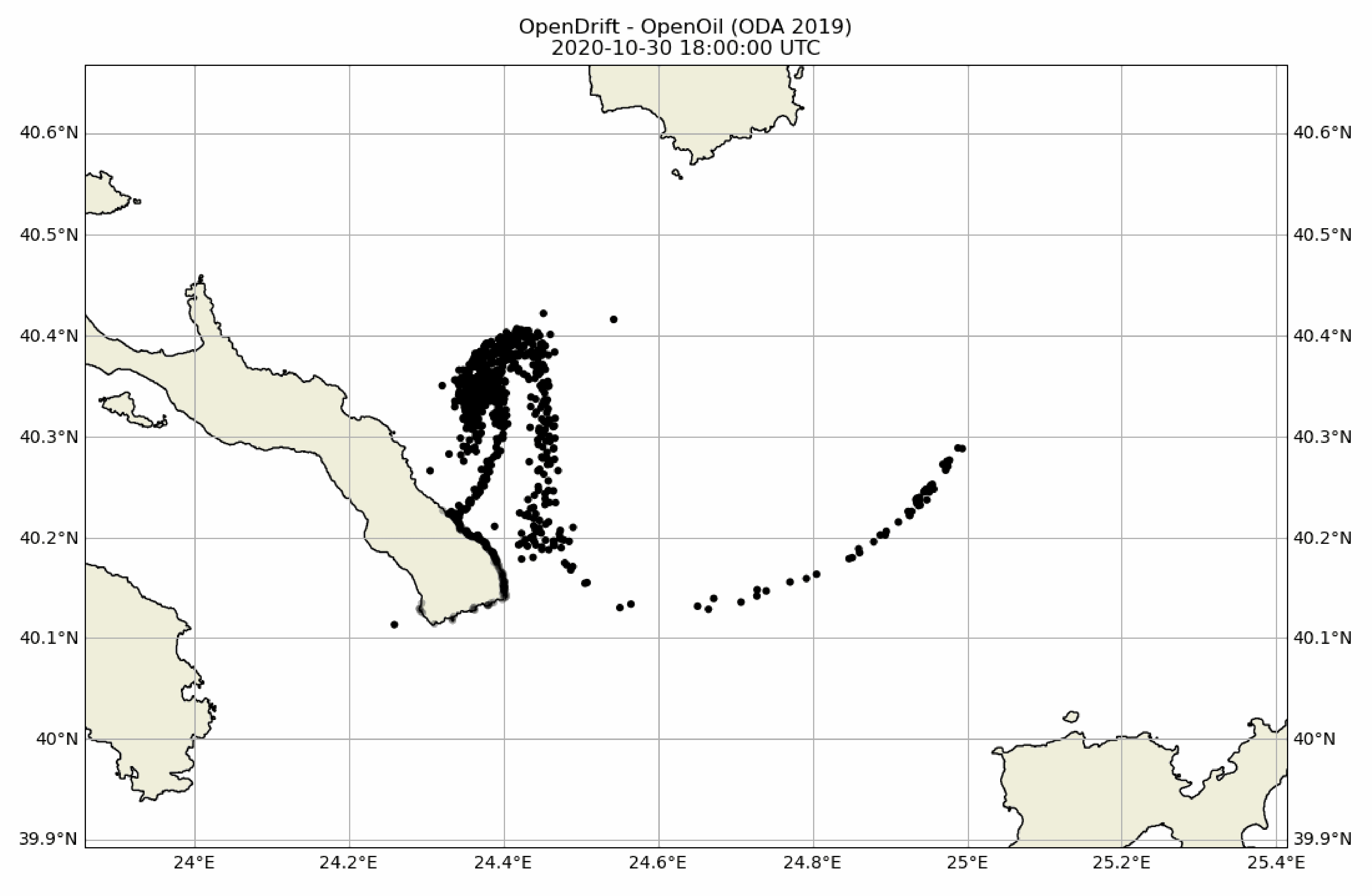
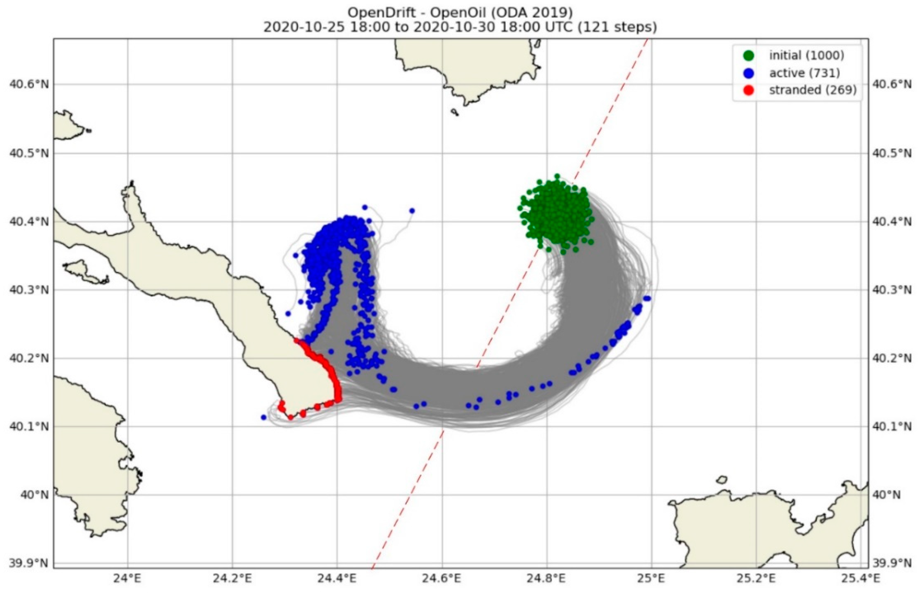
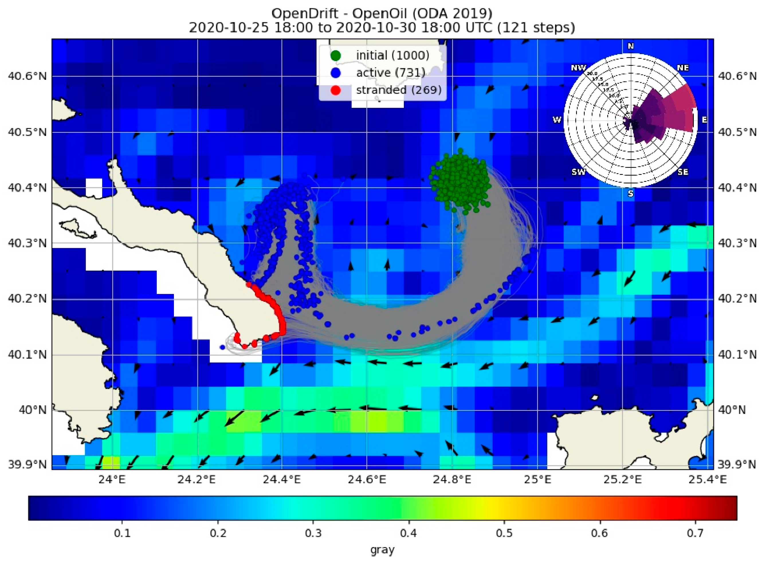
3.1. OpenOil Model Results

This experiment considers that the oil spill is being released from a location between Thassos Island and Athos Peninsula, which belongs to the main tanker route in the area, according to Marine Traffic (https://www.marinetraffic.com (accessed on 12 November 2021)) (Figure 1). During the period of this incident, there was a strong surface current jet with NE–SW direction, with speed varying from 0.1 to 0.25 m/s, transporting the oil particles toward the Athos Peninsula (Figure 2). The wind speed in the area ranged from near-zero to 8.4 m/s (average: 2.53 m/s), blowing from the ENE direction. Wind shear stress and surface currents transferred and dispersed oil particles to the SW. At the end of the 5-day simulation, a significant portion of oil particles (~70%) appeared at the sea area near Athos Peninsula, while the remaining part (~20%) was beached along its coastline, and a small portion of oil elements (<10%) was spread to the east of Athos Peninsula (Supplementary Material, Video S1).

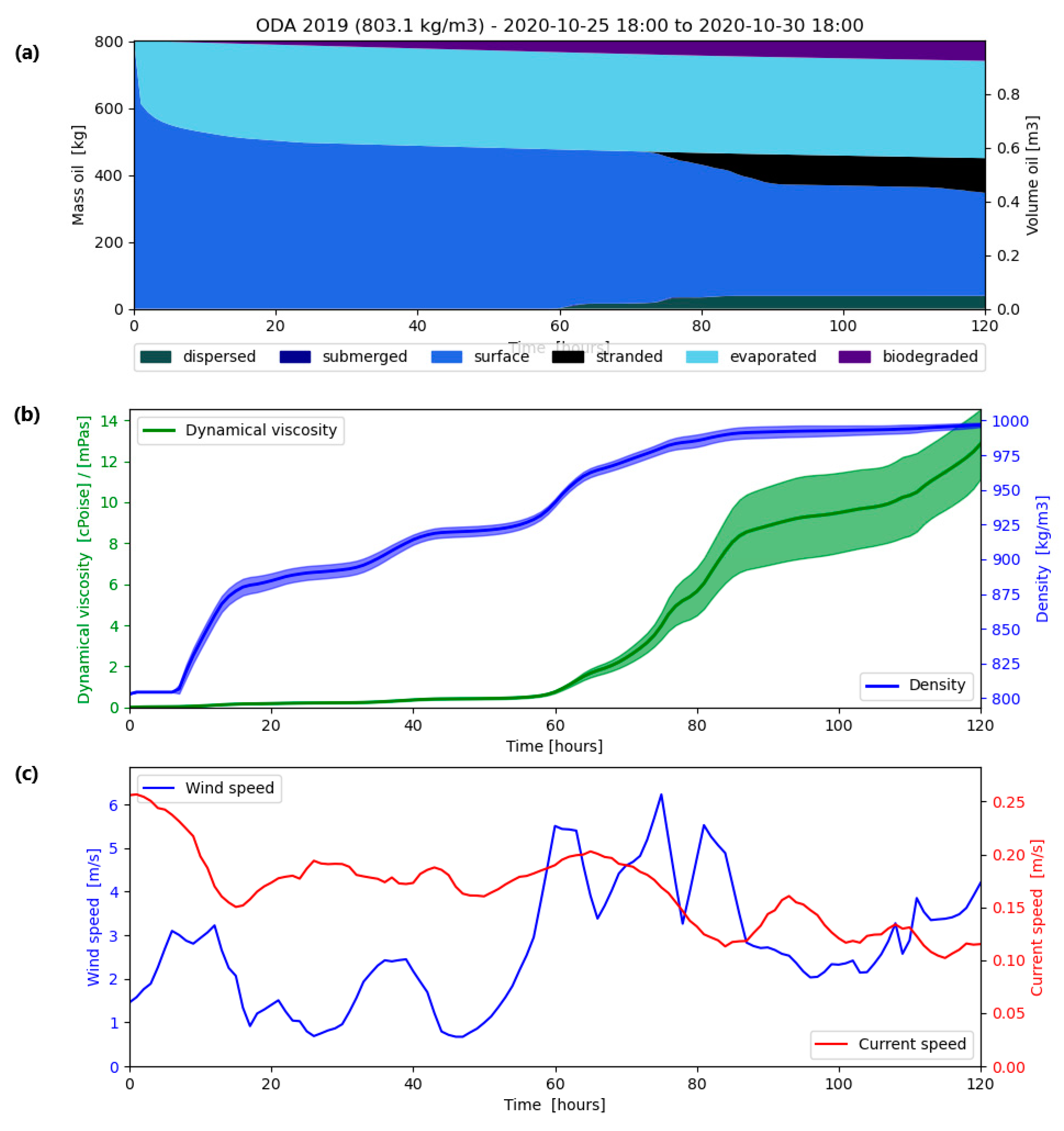
3.2. Oil Budget Analysis

Figure 3a presents the temporal evolution of the dimensionless Weber number (We) contributing to the particle wave entrainment process, as produced by Equation (5). The We number increases substantially after oil release, illustrating the factor of dominance of inertial forces over the oil–water interfacial tension (We ~ 2000 to 6000). In parallel, the time evolution of the Ohnesorge number (Oh), as computed from Equation (7), ranges over the simulation between zero and 14 (Figure 3b). Both numbers show a gradual increase throughout the 5-day experiment, with a sharp rise on Day 3, attributed to the growth of the oil–water interfacial tension. Besides, Figure 3c illustrates the temporal change in the Rayleigh–Taylor (R-T) instability maximum diameter (d_o), as calculated from Equation (6). A continuous growth in this parameter is also shown, doubling rapidly on Day 3 from 0.020 to 0.040 m. The maximum value was noted on the last day of the scenario at 0.045 m.

The oil mass budget per physico-chemical process throughout the simulation time is presented in

Table 2. Mass of oil being evaporated, dispersed and biodegraded.

Percentage (%)/Time (h)	10	20	30	40	50	60	70	80	90	100	110	120
Evaporation (%)	33.63	35.88	36.38	36.38	36.38	36.38	36.38	36.38	36.38	36.38	36.38	36.38
Dispersion (%)	0.00	0.00	0.00	0.00	0.00	0.20	1.96	4.30	4.95	4.96	4.96	4.98
Biodegradation (%)	0.81	1.55	2.28	2.99	3.69	4.38	5.00	5.69	6.25	6.90	7.50	8.00

. The Table illustrates the proportion of oil mass being evaporated, dispersed and biodegraded per 10 h of simulation. The Table shows that 10 h after the initial oil release, approximately 33% of its mass was evaporated, 0.8% of the released oil mass was biodegraded, while all oil particles remained at the sea surface and they had not yet been dispersed in the water column. The above implies that evaporation acts as a short-term process during the first few hours after the oil release. The model results indicate that approximately ~20% of the released oil mass seems to evaporate within the first 24 h, after the occurrence of the incidence. However, as the simulation continues (~60 h from its commencement), the evaporation rate lowers, since ~36% of oil initial mass had been evaporated. Within the same period, the proportion of oil mass being biodegraded increased to 4.4%, while limited oil particles were dispersed into the water column (~0.2%). Finally, at the end of the simulation (120 h), the amount of oil being evaporated remained rather stable, the percentage of dispersed oil particles increased to almost 5%, while the biodegraded particles gradually increased to 8%.

The fact that only a small portion of the released oil mass (<10%) appeared as dispersed after 60 h of simulation seems attributed to the prevailing wave conditions. In this scenario, the simulation was performed with a typical-for-the-season-and-area significant wave height (H_S = 0.5 m). Furthermore, the levels of turbulence at sea surface, resulting from the wind and surface currents and their vertical gradient was also a major factor for vertical oil dispersion. On the contrary, oil biodegradation intensified gradually over time, depicting that this is a complex long-term process. After the first 20 h of the simulation, only a small portion of the dissolved oil seemed to be biodegraded, increasing gradually over time, and finally reaching about 5% of the total oil mass. As the wind speed increased (after 110 h from the release), a significant portion of the submerged oil resurfaced. In parallel, as the incident evolved, the number of oil particles that adhered to the shores increased; thus, after about 70 h, the beached oil reached ~20% of its initial mass (Figure 4a).

As the oil mass balance evolved after oil release, oil properties changed in time, and thus, as shown in Figure 4b, the dynamic oil viscosity remained almost stable over the first 60 h of the simulation, reaching near-zero levels, but rising again, right after the first 120 h, until the maximum dynamic viscosity value ~14 cPoise (Figure 4b). Furthermore, the simulation shows that although the initial oil density was 800 kg m⁻³, at the first 24 h of simulation, it approached ~900 kg m⁻³. Then, oil density exhibited a steady increase until Day 3 of the experiment, when it reached 1000 kg m⁻³ (Figure 4b). These results represent changes in the physicochemical properties of the oil type “ODA 2019”; different results could have been obtained if another oil type was used in this experimental simulation. These results are related to the speed of the winds and ocean currents (Figure 4c). Three days after the oil release, the wind speed increased rapidly from 1 to 5–6 m/s, while sea surface currents were approximately 0.20 m/s. The introduction of turbulence affected the wave entrainment (through Equation (4)), oil resurfacing (through Equation (9)) and vertical turbulent mixing (through Equation (10)), thus affecting the total number of oil particles being dispersed in the water column.

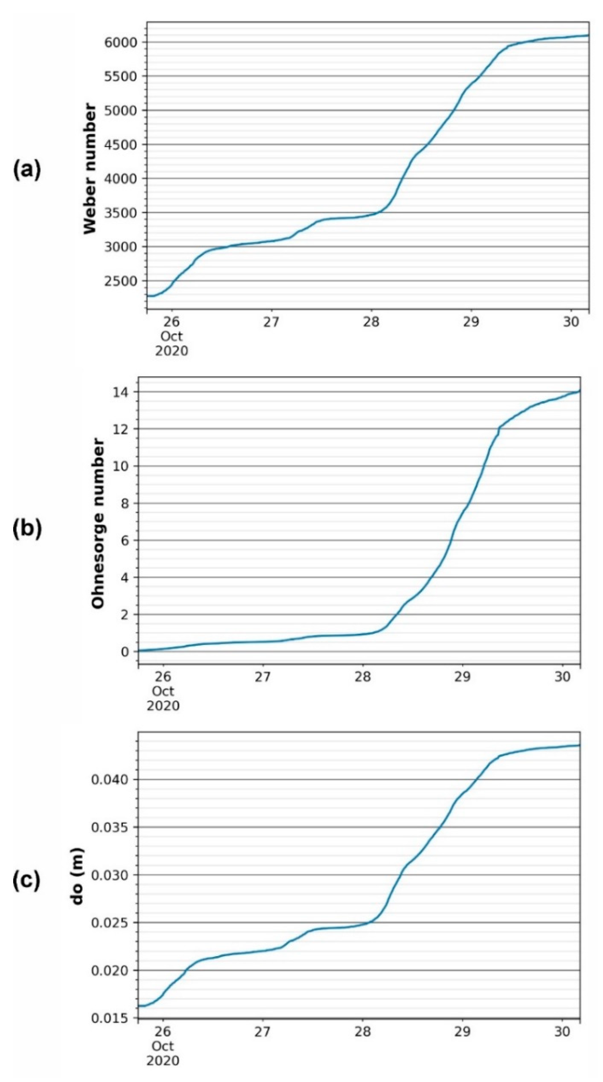
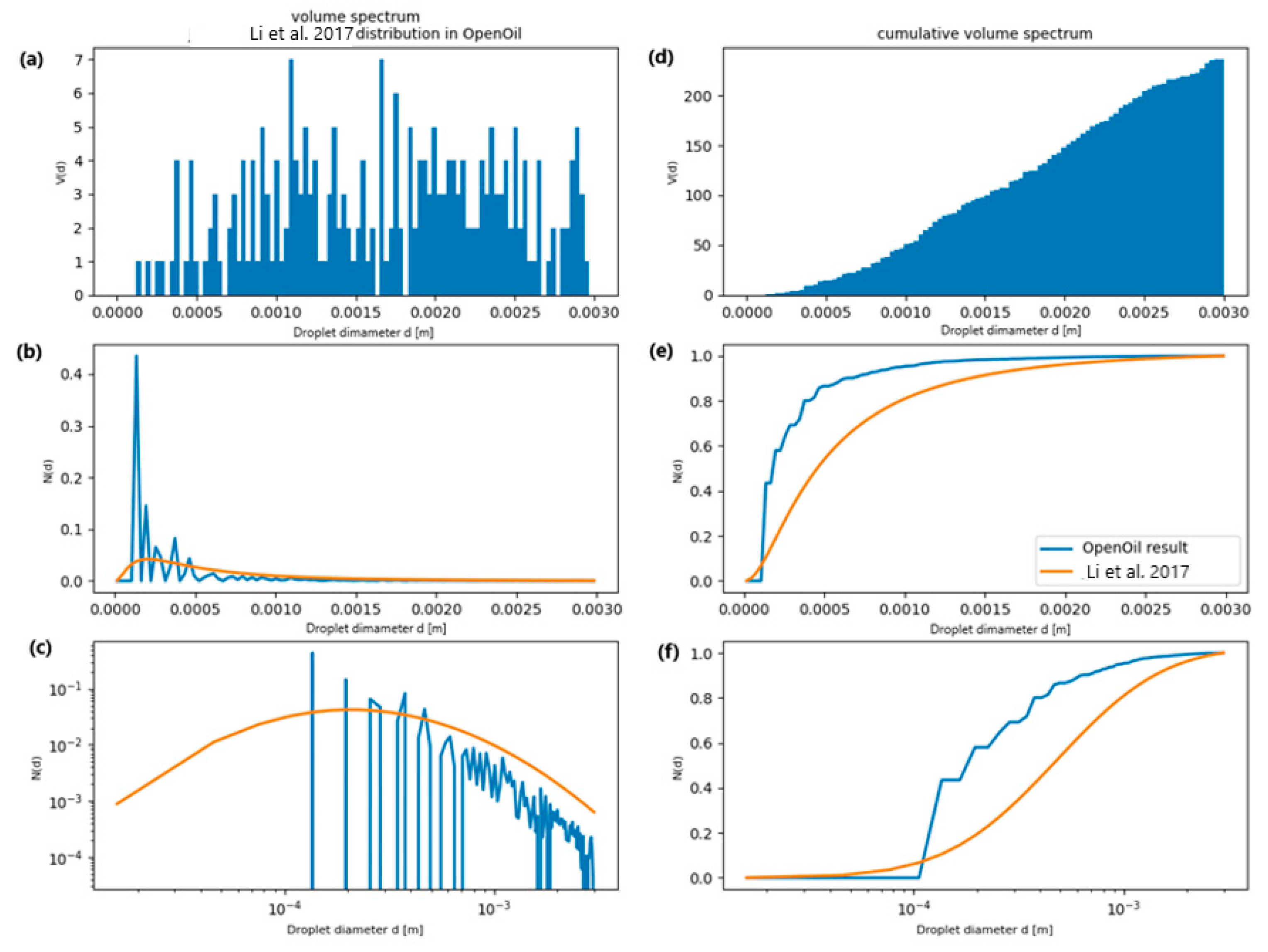
3.3. Oil Droplets’ Size Spectrum

Despite the fact that the droplet size spectrum is associated with the stochastic wave entrainment schemes, depending on oil properties and environmental conditions (Equation (17)), the droplet size distribution of all submerged particles changed dynamically due to two factors: First, oil properties alter over the simulation, producing various spectra due to wave entrainment effects. Second, oil droplets rise to the sea surface at various speeds, depending on the droplet size. Figure 5c illustrates the resulting droplet size distribution at the end of the simulation. For oil particles, a simplistic and pragmatic scheme of prescribing random radii in the range of 0.1 to 1 mm was used according to Li et al. [18]. The blue line illustrates the oil droplet distribution according to the droplet diameter computed by the OpenOil model, while the orange line represents the approximation of Li et al. [18].

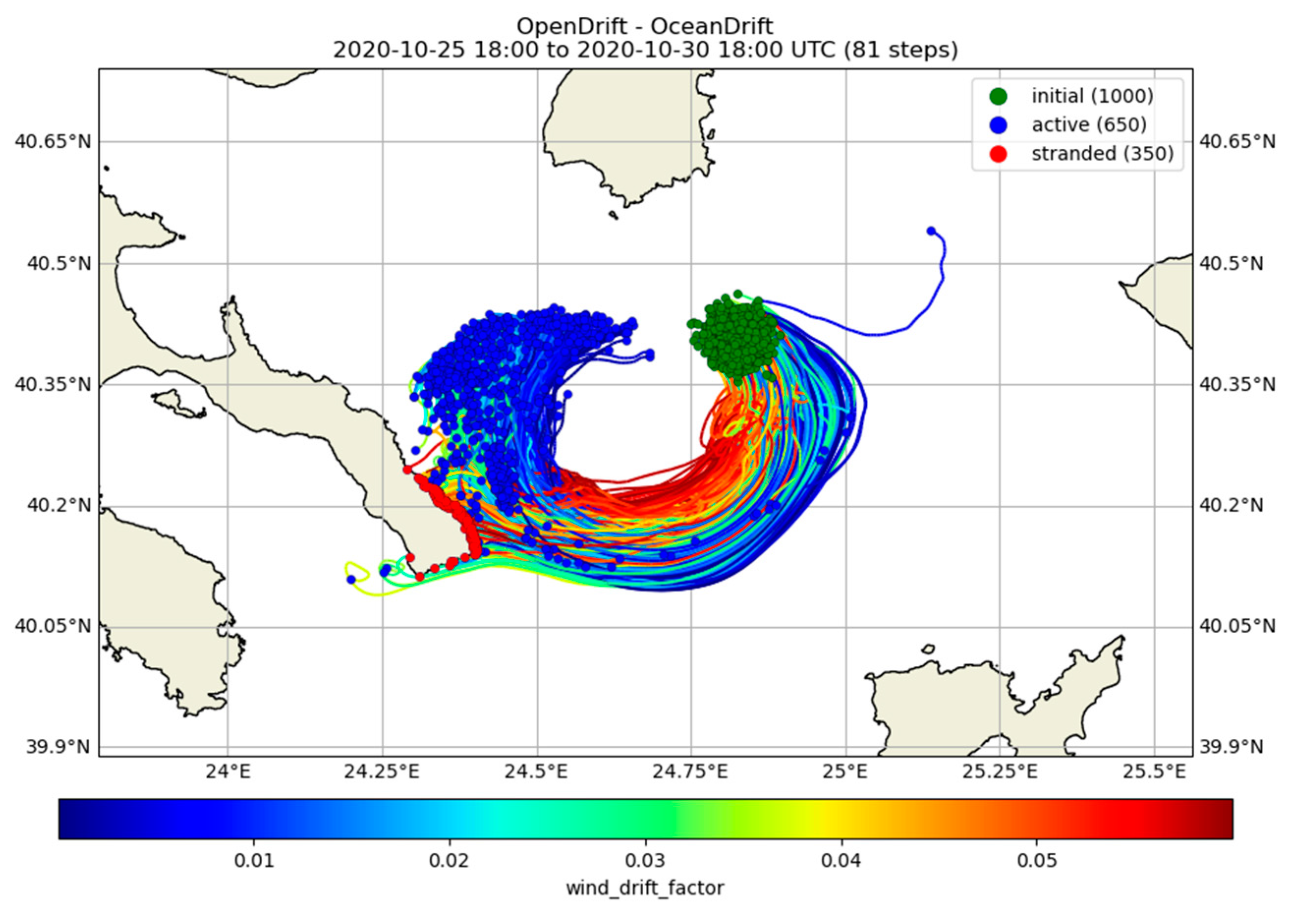
3.4. Wind Drift Analysis

The wind drift factor, which is important for the horizontal motion of oil elements, is linearly proportional to the wind speed acting on the sea surface, ranging from approximately 1% to 6% (Figure 6). As particles follow an anticyclonic eddy-like trajectory, higher wind drift (~6% of wind speed) is applied at the northern, internal radii of the system and intermediate drifts at the southern, external trajectories (~3%), while lower drifts affect the bulk of the particles. This appears to be a dominant factor in determining the final fate of the particles, since particles moving along the external radius of the eddy had a higher probability to be stranded on the Athos Peninsula. Conversely, particles at the central and internal trajectories of the eddy system avoided beaching and remain active until the end of the simulation.

3.5. Oil Particles Dispersion

To better understand the behavior of the oil particles’ cloud along their trajectory, under the influence of horizontal currents and winds, the horizontal dispersion coefficient, K, and its constituents along (K_x) and across (K_y) the central pathway of the oil spill were calculated at each computational time step. According to the convention followed, positive K-values indicate oil spill spreading and movement of particles away from the longitudinal and transverse central flow of the oil spill trajectory, designating oil spill spreading, while negative values indicate oil spill compression and movement of particles toward the central trajectory line.

In parallel, turbulent kinetic energy (TKE) is expected to play a dominant role in particle distribution along and across the main oil spill’s pathway. Figure 7 presents the time dependence of the dispersion coefficient, K, and the turbulent kinetic energy, TKE, of oil particles over 10 semi-diurnal tidal cycles, representing the 5-day simulation period. Since the beginning of the simulation, there was a small increase in both the dispersion coefficient, K, and the turbulent kinetic energy, TKE, from 0 to 50 m²/s and from 0.003 to 0.004 m²/s², respectively. During this phase, particles moved to the S–SE direction, toward the Athos Peninsula. After 5 tidal cycles, the oil spill moved westward, and intense fluctuation occurred, increasing K to 200 m²/s and TKE to 0.005 m²/s². Then, a sharp decrease was observed during the third day of the simulation (tidal cycles 6–7), when the dispersion coefficient reached negative values of −100 m²/s² and the TKE decreased to 0.0035 m²/s². This event coincided with a change in the direction of motion of the oil particles, from W to NW. The negative values in the dispersion coefficient, K, imply that the oil elements traveled in the negative x-direction; thus, the oil cloud compressed toward its center of gravity. Furthermore, on Day 4 of the simulation (tidal cycle 8), a significant increase was observed in the dispersion effects (up to 150 m²/s) due to the introduced turbulent energy (up to 0.006 m²/s²).

Our results indicate that the distribution of K was mostly affected by the along-flow particles dispersion, thus from K_x, rather than from the K_y-component. Figure 8 illustrates the time dependence of the effective longitudinal dispersion coefficient, K_x, and the respective longitudinal turbulent kinetic energy, TKE_x, over the 10 tidal cycles of the 5-day simulation period. At the commencement of the simulation, K_x increased steadily from 0 to 100 m²/s, as TKE_x changed from 3 to 4 × 10⁻³ m²/s². After the completion of 5 tidal cycles, the dominant surface flow had strong magnitude and was from the SE direction, increasing TKE_x up to 8 × 10⁻³ m²/s², and leading oil particles to exhibit an intense fluctuation in the along-flow direction (K_x up to 700 m²/s). As the direction of oil spill motion changed from SE to W during tidal cycles 6–7, the level of turbulence reduced (TKE_x ~ 3 × 10⁻³ m²/s²) and the oil spill contracted in the along-flow direction (K_x ~ −500 m²/s). The along-flow current and TKE reduction seemed responsible for the beaching of particles, moving due to inertia forces toward the shore. Finally, during the three final tidal cycles, and after the change in patch direction to the NW, TKE_x rose again toward 8 × 10⁻³ m²/s² and the along-flow dispersion grew to 500 m²/s.

Similarly, the transverse dispersion coefficient, K_y, exhibited low fluctuation levels (from zero to 100 m²/s) during the first tidal cycles of simulation, guided by the limited TKE_y ranging from 2.5 × 10⁻³ to 3.0 × 10⁻³ m²/s². As the flow intensified in tidal cycle 3, K_y and TKE_y stabilized at 200 and 4 × 10⁻³ m²/s², respectively. Then, a sharp decrease in both parameters was observed, reaching 0 m²/s for K_y and 3 × 10⁻³ m²/s² for TKE_y. This pattern was repeated every two tidal cycles, with the maximum value for K_y at 300 m²/s (after 8 tidal cycles) and for TKE_y 6 × 10⁻³ m²/s² (after 10 tidal cycles) (Figure 9).

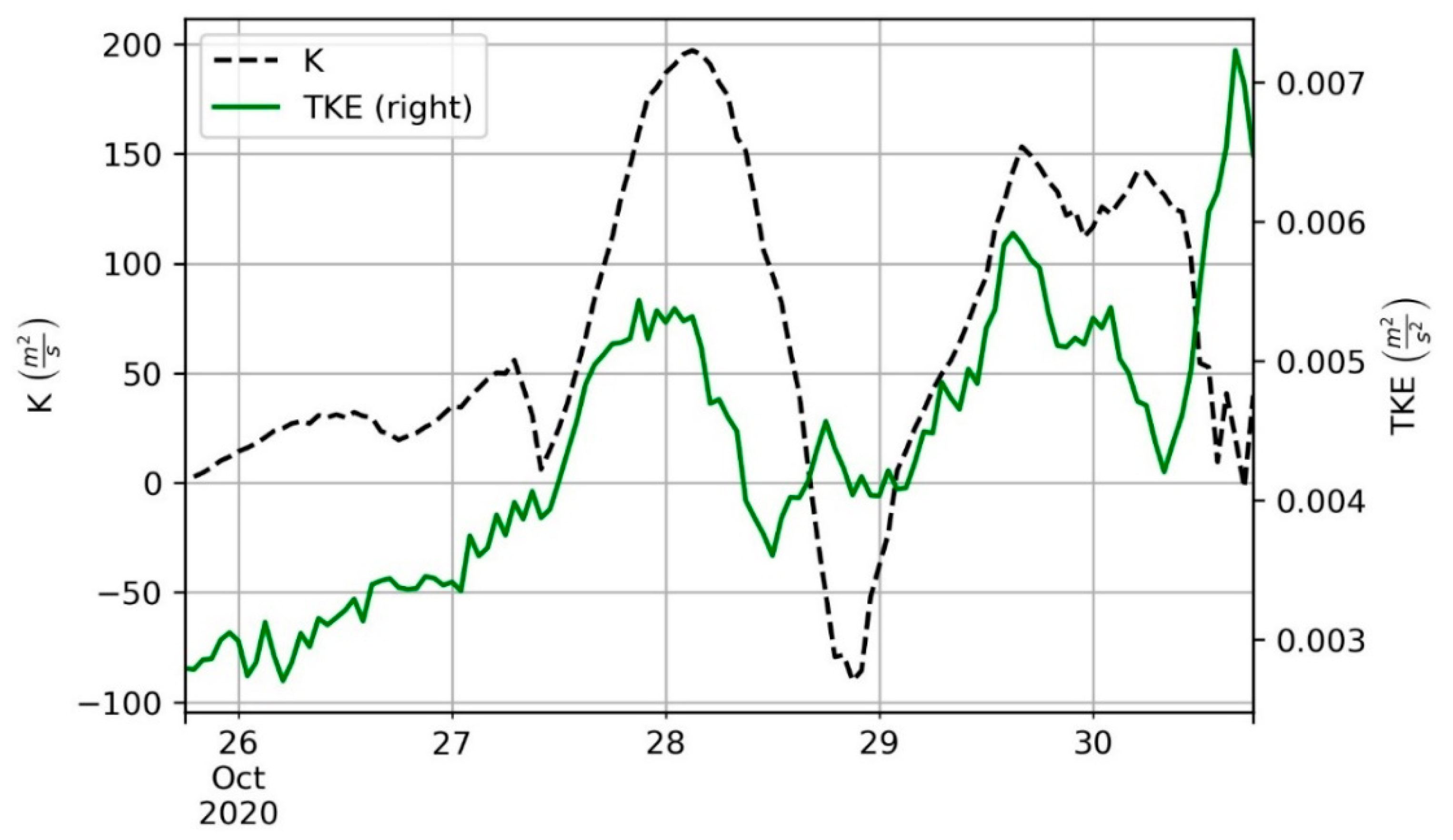
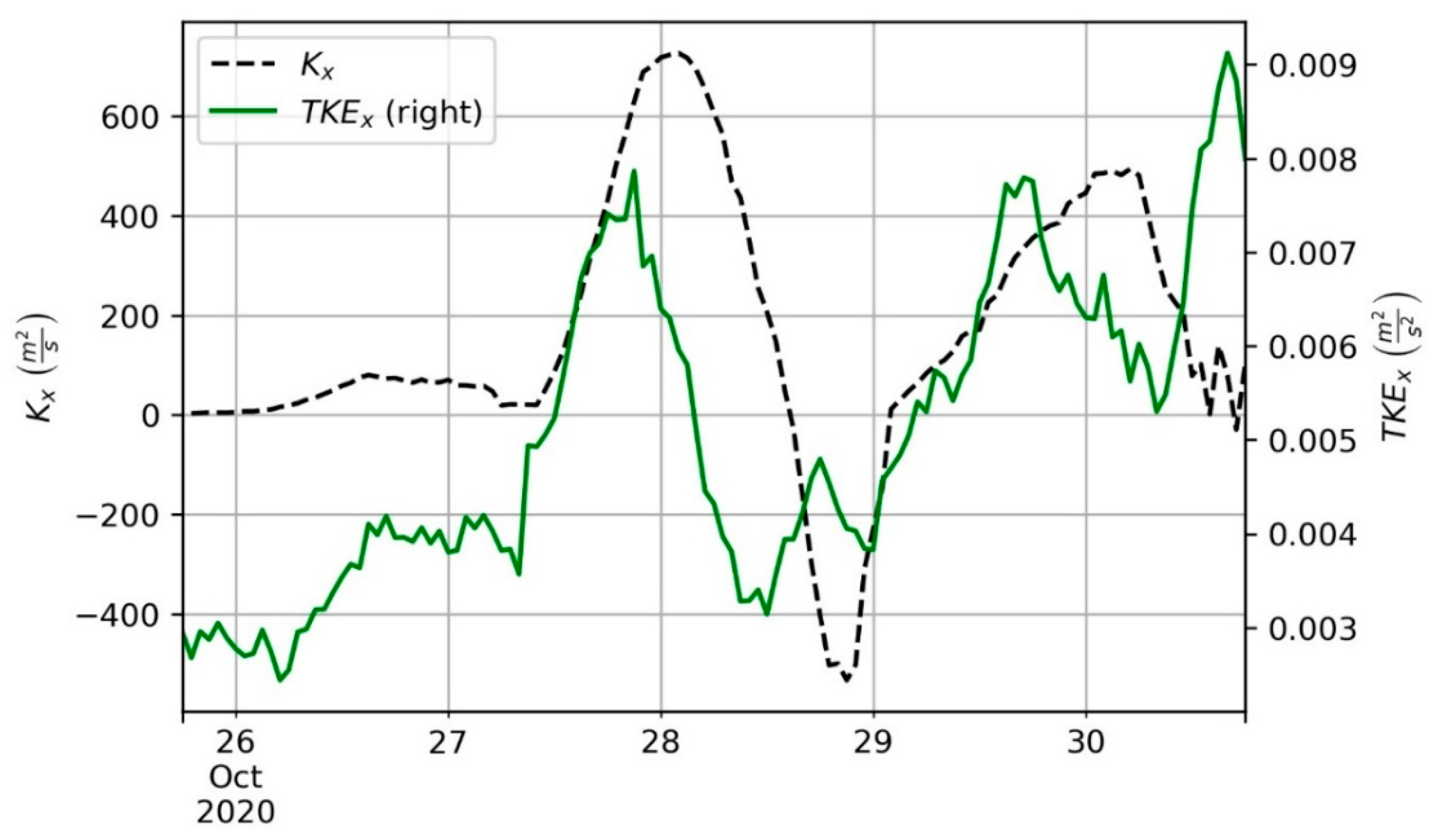
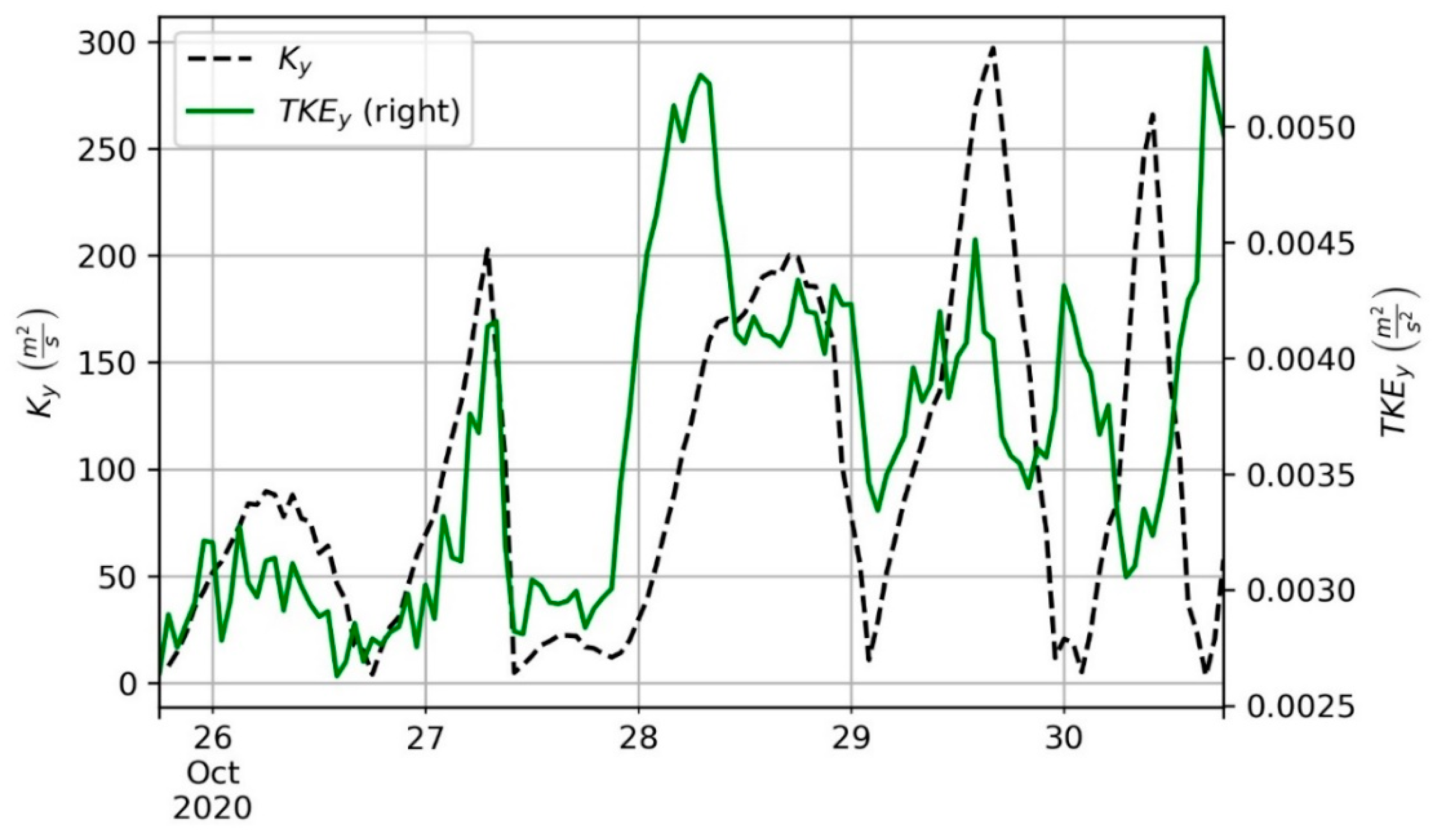
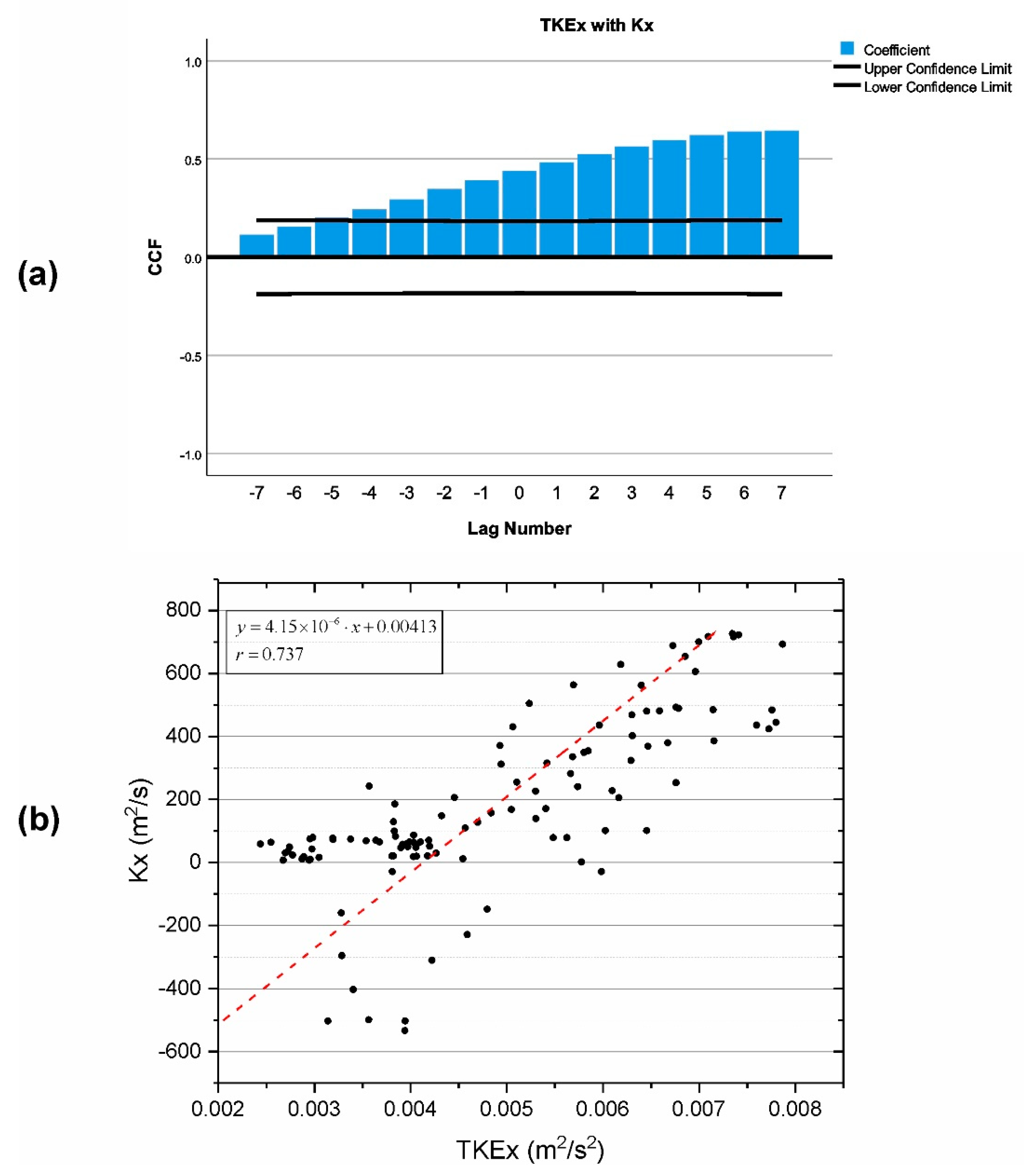
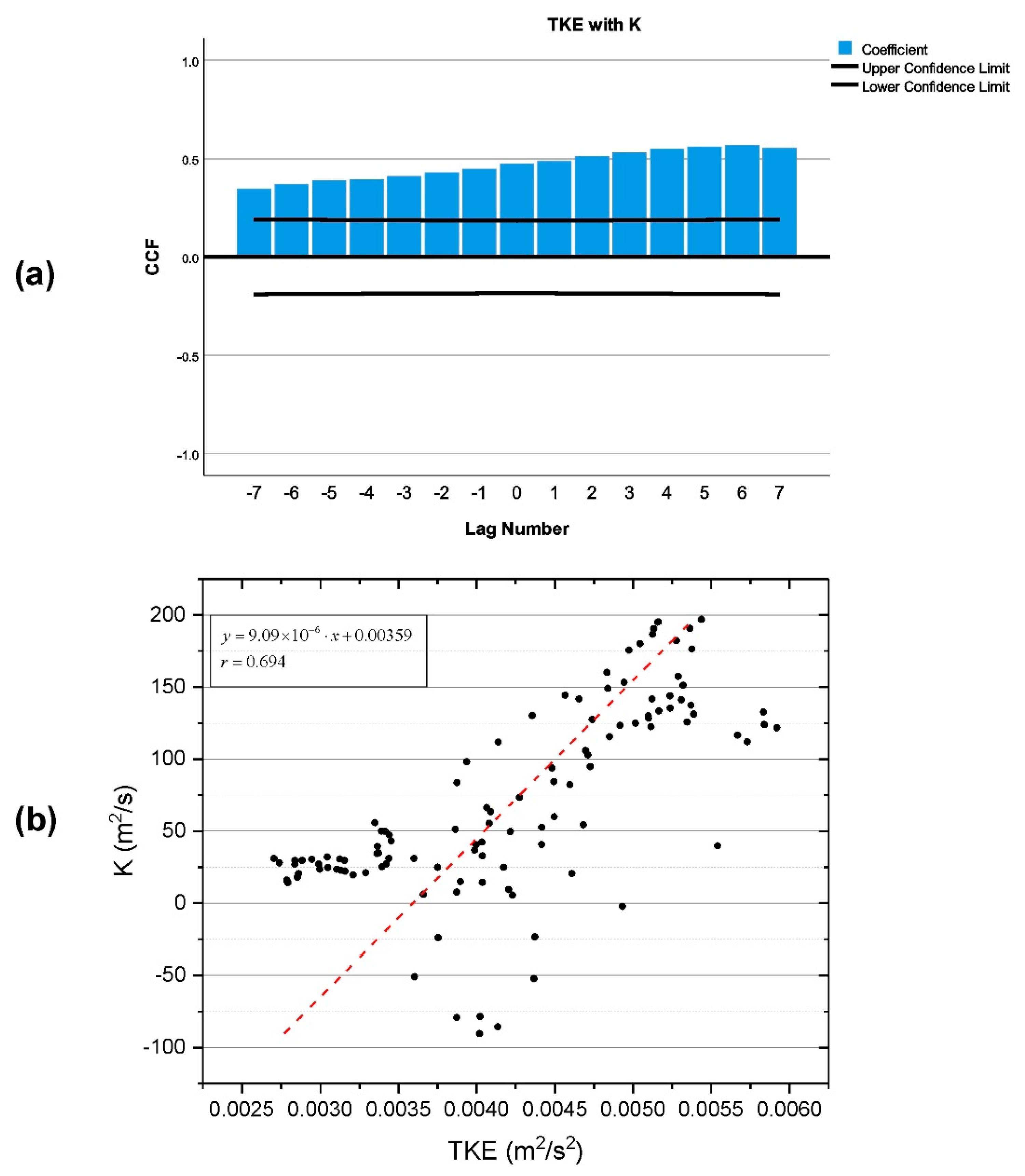
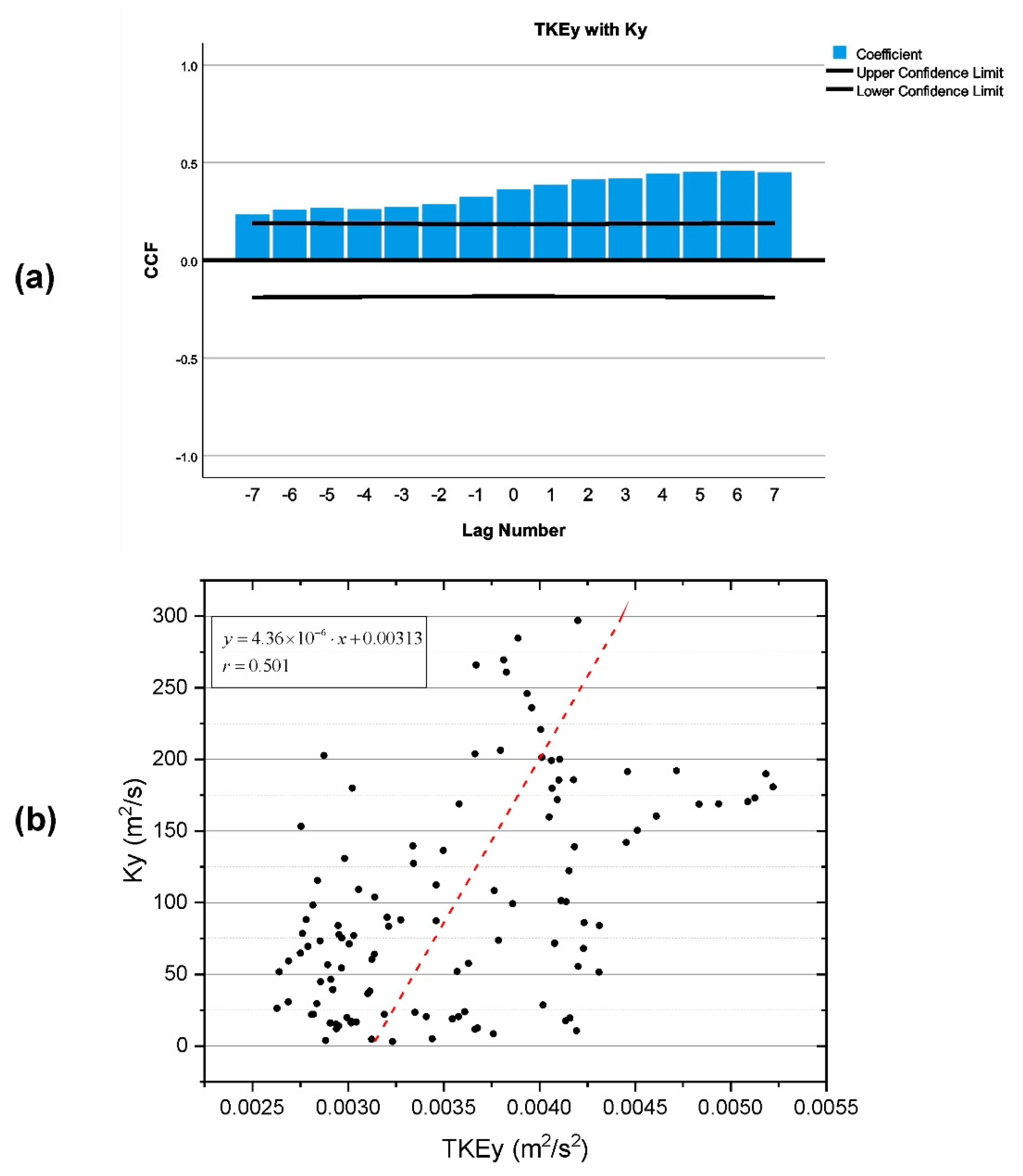
3.6. TKE Impact on Oil Dispersion

As analyzed earlier, the temporal evolution of TKE affected the expansion and shrinking of the oil spill, expressed by the cloud of particles moving horizontally at the sea surface. Both curves appear relatively synchronous, with TKE leading the changes and the K-parameter following. Cross-correlation analysis on the hourly time-series of both parameters illustrates that the strongest correlation occurred at lag 6, implying that TKE affects the particles dispersion 6 h after its rise (Figure 10a). The cross-correlation coefficient at lag = 6 equals 0.568, which proves that the turbulent kinetic energy, TKE, and the dispersion coefficient, K, are strongly contemporaneously correlated. The scatterplot of 6 h lagged K to TKE exhibits Pearson’s correlation coefficient of 0.694 (Figure 10b).

The strongest correlation between the turbulent kinetic energy, TKE, and the dispersion, K, is found in the longitudinal direction of oil particles movement. The cross-correlation coefficient between TKE_x and K_x was estimated at 0.644, occurring at lag 7 (time difference of 7 h), as seen in Figure 11a. This significant positive correlation illustrates that the horizontal along-flow currents exert significant impacts on the shape of the oil spill, deforming the patch along the longitudinal axis of its movement. However, the present wind and current speeds need approximately 7 h to produce such a deformation. The scatterplot of the 7 h lagged K_x in relation to TKE_x shows a Pearson correlation coefficient of 0.737 (Figure 11b).

Finally, the cross-correlation analysis reveals that the transversal dispersion, i.e., the movement of oil particles away from the main axis of longitudinal flow, is moderately affected by the cross-flow TKE, since r_K,TKE = 0.457, with a time lag of 6 h and a Pearson coefficient of 0.501 (Figure 12).

4. Conclusions

In this work, we have presented the simulation of an oil spill transport and dispersion, released along the main tanker route in the North Aegean Sea, using the widely used, open-source numerical model OpenOil. The model was coupled with meteorological data from NOAA GFS and with hydrodynamic data from CMEMS. The influence of the prevailing winds and surface currents were responsible for oil transport and spreading. Oil weathering processes, such as evaporation, dispersion and biodegradation were also significant, although they acted at different rates and time scales. In general, from the above simulation scenario, it was observed that the largest percentage of the oil mass remained at the sea surface, namely 60% at the beginning of the simulation and about 40% at the end of the simulation. At the same time, a large percentage evaporated from the first hours (~40%), while a small percentage adhered to the shores (~20%), biodegraded (<8%) and dispersed (<5%) by the end of the simulation. In addition, the effects of wind, dynamic viscosity and physicochemical processes were observed, as after the first 60 h and as the winds in the area intensified, the dispersion of oil in the water column commenced, in parallel to the stranding of the oil mass portion on the coast.

By examining the displacement of particles over the flow field for multiple tidal periods, the basic features of the oil spill transport pattern in the area were revealed. As previously analyzed, the evolution of TKE affected the expansion and contraction of the oil slick, expressed by the oil droplets moving horizontally at the sea surface. The distribution of the dispersion coefficient, K, was found to be mostly affected by K_x than by K_y, explaining that the along-flow deformation of the spill was more evident. It was also noted that as turbulence and turbulent kinetic energy developed, the dispersion of the oil particles was more pronounced, with a time lag of 6–7 h. Based on the above analysis, and particularly the linear regressions applied between TKE and K, the forecasted levels of TKE could be used to predict the deformation of the oil spill along and across its trajectory. This is particularly important for response and contingency planning, as the background turbulence affects the spreading and expansion of the oil spill.

Future work will involve firstly the operational coupling of OpenOil with the forecasted winds, waves, 3D currents and water column dynamics, as produced by the coupled, high-resolution models of the ODYSSEA project (Delft3D-FLOW, AEM, SWAN) and secondly the improvement in the parameterization of oil weathering processes, such as biodegradation.

References

1. Brekke, C.; Solberg, A.H.S. Oil spill detection by satellite remote sensing. Remote Sens. Environ. 2005, 95, 1–13. [Google Scholar] [CrossRef]
2. Dietrich, J.C.; Trahan, C.J.; Howard, M.T.; Fleming, J.G.; Weaver, R.J.; Tanaka, S.; Yu, L.; Luettich, R.A.; Dawson, C.N.; Westerink, J.J.; et al. Surface trajectories of oil transport along the Northern Coastline of the Gulf of Mexico. Cont. Shelf Res. 2012, 41, 17–47. [Google Scholar] [CrossRef]
3. Alves, T.M.; Kokinou, E.; Zodiatis, G. A three-step model to assess shoreline and offshore susceptibility to oil spills: The South Aegean (Crete) as an analogue for confined marine basins. Mar. Pollut. Bull. 2014, 86, 443–457. [Google Scholar] [CrossRef] [PubMed]
4. Alves, T.M.; Kokinou, E.; Zodiatis, G.; Lardner, R.; Panagiotakis, C.; Radhakrishnan, H. Modelling of oil spills in confined maritime basins: The case for early response in the Eastern Mediterranean Sea. Environ. Pollut. 2015, 206, 390–399. [Google Scholar] [CrossRef] [PubMed] [Green Version]
5. Alves, T.M.; Kokinou, E.; Zodiatis, G.; Radhakrishnan, H.; Panagiotakis, C.; Lardner, R. Multidisciplinary oil spill modeling to protect coastal communities and the environment of the Eastern Mediterranean Sea. Sci. Rep. 2016, 6, 36882. [Google Scholar] [CrossRef]
6. Yang, H.; Hong, B.; Chen, S. Research and application progress of marine oil-spill models. Trans. Oceanol. Limnol. 2007, 2, 156–163. [Google Scholar]
7. Holmes, O. ‘It’ll Take Decades to Clean’: Oil Spill Ravages East Mediterranean. Available online: https://www.theguardian.com/world/2021/feb/22/take-decades-clean-oil-spill-oil-spill-ravages-east-mediterranean (accessed on 22 February 2021).
8. Gerretsen, I. Mauritius Oil Spill: Questions Mount over Ship Fuel Safety. Available online: https://www.climatechangenews.com/2021/02/19/mauritius-oil-spill-raises-concerns-ship-fuel-safety/ (accessed on 19 February 2021).
9. Kourdi, E.; Salem, M.; Qiblawi, T. Syrian Oil Spill Spreads across the Mediterranean. Available online: https://www.cnn.com/2021/08/31/middleeast/syria-cyprus-oil-spill-intl/index.html (accessed on 9 January 2021).
10. Blevins, G.; Allen, J. ‘Catastrophic’ California Oil Spill Kills Fish, Damages Wetlands. Available online: https://www.reuters.com/world/us/major-oil-spill-washes-ashore-california-killing-wildlife-2021-10-03/ (accessed on 5 October 2021).
11. Fingas, M.; Fieldhouse, B. Water-in-Oil Emulsions: Formation and Prediction. In Handbook of Oil Spill Science and Technology; John Wiley & Sons, Inc.: Hoboken, NJ, USA, 2015; Volume 225, pp. 225–270. [Google Scholar] [CrossRef]
12. Azevedo, A.; Oliveira, A.; Fortunato, A.B.; Zhang, J.; Baptista, A.M. A cross-scale numerical modeling system for management support of oil spill accidents. Mar. Pollut. Bull. 2014, 80, 132–147. [Google Scholar] [CrossRef]
13. Keramea, P.; Spanoudaki, K.; Zodiatis, G.; Gikas, G.; Sylaios, G. Oil spill modeling: A critical review on current trends, perspectives, and challenges. J. Mar. Sci. Eng. 2021, 9, 181. [Google Scholar] [CrossRef]
14. Barker, C.H.; Kourafalou, V.H.; Beegle-Krause, C.J.; Boufadel, M.; Bourassa, M.A.; Buschang, S.G.; Androulidakis, Y.; Chassignet, E.P.; Dagestad, K.F.; Danmeier, D.G.; et al. Progress in operational modeling in support of oil spill response. J. Mar. Sci. Eng. 2020, 8, 668. [Google Scholar] [CrossRef]
15. Zhong, Z.; You, F. Oil spill response planning with consideration of physicochemical evolution of the oil slick: A multiobjective optimization approach. Comput. Chem. Eng. 2011, 35, 1614–1630. [Google Scholar] [CrossRef]
16. Röhrs, J.; Dagestad, K.-F.; Asbjørnsen, H.; Nordam, T.; Skancke, J.; Jones, C.E.; Brekke, C. The effect of vertical mixing on the horizontal drift of oil spills. Ocean. Sci. 2018, 14, 1581–1601. [Google Scholar] [CrossRef] [Green Version]
17. Dagestad, K.F.; Röhrs, J.; Breivik, O.; Ådlandsvik, B. OpenDrift v1.0: A generic framework for trajectory modelling. Geosci. Model Dev. 2018, 11, 1405–1420. [Google Scholar] [CrossRef] [Green Version]
18. Li, C.; Miller, J.; Wang, J.; Koley, S.S.; Katz, J. Size distribution and dispersion of droplets generated by impingement of breaking waves on oil slicks. J. Geophys. Res. Ocean. 2017, 122, 7938–7957. [Google Scholar] [CrossRef]
19. Visser, A.W. Using random walk models to simulate the vertical distribution of particles in a turbulent water column. Mar. Ecol. Prog. Ser. 1997, 158, 275–281. [Google Scholar] [CrossRef] [Green Version]
20. Tkalich, P.; Chan, E.S. Vertical mixing of oil droplets by breaking waves. Mar. Pollut. Bull. 2002, 44, 1219–1229. [Google Scholar] [CrossRef]
21. Hole, L.R.; Dagestad, K.-F.; Röhrs, J.; Wettre, C.; Kourafalou, V.H.; Androulidakis, Y.; Kang, H.; le Hénaff, M.; Garcia-Pineda, O. The deepwater horizon oil slick: Simulations of river front effects and oil droplet size distribution. J. Mar. Sci. Eng. 2019, 7, 329. [Google Scholar] [CrossRef] [Green Version]
22. Lehr, W.; Jones, R.; Evans, M.; Simecek-Beatty, D.; Overstreet, R. Revisions of the ADIOS oil spill model. Environ. Model. Softw. 2002, 17, 189–197. [Google Scholar] [CrossRef]
23. Jones, C.E.; Dagestad, K.F.; Breivik, Ø.; Holt, B.; Röhrs, J.; Christensen, K.H.; Espeseth, M.; Brekke, C.; Skrunes, S. Measurement and modeling of oil slick transport. J. Geophys. Res. Ocean. 2016, 121, 7759–7775. [Google Scholar] [CrossRef]
24. Androulidakis, Y.; Kourafalou, V.; Hole, L.R.; Hénaff, M.L.; Kang, H.S. Pathways of oil spills from potential cuban offshore exploration: Influence of ocean circulation. J. Mar. Sci. Eng. 2020, 8, 535. [Google Scholar] [CrossRef]
25. Brekke, C.; Espeseth, M.M.; Dagestad, K.F.; Röhrs, J.; Hole, L.R.; Reigber, A. Integrated analysis of multisensor datasets and oil drift simulations—A free-floating oil experiment in the open ocean. J. Geophys. Res. Ocean. 2021, 126, e2020JC016499. [Google Scholar] [CrossRef]
26. Kenyon, K.E. Stokes drift for random gravity waves. J. Geophys. Res. 1969, 74, 6991–6994. [Google Scholar] [CrossRef]
27. Ardhuin, F.; Marié, L.; Rascle, N.; Forget, P.; Roland, A. Observation and estimation of lagrangian, stokes, and Eulerian currents induced by wind and waves at the sea surface. J. Phys. Oceanogr. 2009, 39, 2820–2838. [Google Scholar] [CrossRef]
28. Lamarre, E.; Melville, W.K. Air entrainment and dissipation in breaking waves. Nature 1991, 351, 469–472. [Google Scholar] [CrossRef]
29. Delvigne, G.A.L.; Sweeney, C.E. Natural dispersion of oil. Oil Chem. Pollut. 1989, 4, 281–310. [Google Scholar] [CrossRef]
30. Delvigne, G.A.L.; Hulsen, L.J.M. Simplified Laboratory Measurements of Oil Dispersion Coefficient Application in Computations of Natural Oil Dispersion. In Proceedings of the Seventeenth Arctic and Marine Oil Spill Program (AMOP) Technical Seminar, Vancouver, BC, Canada, 8–10 June 1994; Volume 1, pp. 173–187. [Google Scholar]
31. Reed, M.; Turner, C.; Odulo, A. The role of wind and emulsification in modelling oil spill and surface drifter trajectories. Spill Sci. Technol. Bull. 1994, 1, 143–157. [Google Scholar] [CrossRef]
32. Holthuijsen, L.H.; Herbers, T.H.C. Statistics of breaking waves observed as whitecaps in the open sea. J. Phys. Oceanogr. 1986, 16, 290–297. [Google Scholar] [CrossRef] [Green Version]
33. Reed, M.; Johansen, O.; Leirvik, F.; Brørs, B. Numerical algorithm to compute the effects of breakingwaves on surface oil spilled at sea. Final. Rep. Submitt. Coast. Response Res. Center Rep. F 2009, 10968, 131. [Google Scholar]
34. Grace, J.R.; Wairegi, T.; Brophy, J. Break-up of drops and bubbles in stagnant media. Can. J. Chem. Eng. 1978, 56, 3–8. [Google Scholar] [CrossRef]
35. Ohnesorge, W.V. Formation of Drops by Nozzles and the Breakup of Liquid Jets; Mech: Berlin, Germany, 1936; Volume 16, pp. 355–358. [Google Scholar]
36. Lefebvre, A.H.; McDonell, V.G. Atomization and Sprays; CRC Press: Boca Raton, FL, USA, 2017; pp. 1–284. [Google Scholar] [CrossRef]
37. Raj, P.P.K. Theoretical Study to Determine the Sea State Limit for the Survival of Oil Slicks on the Ocean; Little (Arthur D) Inc.: Cambridge, MA, USA, 1977. [Google Scholar]
38. Thygesen, U.H.; Ådlandsvik, B. Simulating vertical turbulent dispersal with finite volumes and binned random walks. Mar. Ecol. Prog. Ser. 2007, 347, 145–153. [Google Scholar] [CrossRef] [Green Version]
39. Johansen, Ø.; Reed, M.; Bodsberg, N.R. Natural dispersion revisited. Mar. Pollut. Bull. 2015, 93, 20–26. [Google Scholar] [CrossRef]
40. Stiver, W.; Mackay, D. Evaporation rate of spills of hydrocarbons and petroleum mixtures. Environ. Sci. Technol. 1984, 18, 834–840. [Google Scholar] [CrossRef] [PubMed]
41. Jones, R.K. A Simplified Pseudo-Component Oil Evaporation Model. In Proceedings of the 20th Arctic and Marine Oil Spill Program Technical Seminar, Vancouver, BC, Canada, 11–13 June 1997; pp. 43–61. [Google Scholar]
42. Lyman, W.J.; Reehl, W.F.; Rosenblatt, D.H. Handbook of Chemical Property Estimation Methods: Environmental Behavior of Organic Compounds; American Chemical Society: Washington, DC, USA, 1990. [Google Scholar]
43. Mackay, D.; Buist, I.; Mascarenhas, R.; Patterson, S. Oil Spill Processes and Models; Technical Report No. EE/8; Environ. Can.: Ottawa, ON, Canada, 1980; 17p. [Google Scholar]
44. Eley, D.D.; Hey, M.J.; Symonds, J.D. Emulsions of water in asphaltene-containing oils 1. Droplet size distribution and emulsification rates. Colloids Surf. 1988, 32, 87–101. [Google Scholar] [CrossRef]
45. Ławniczak, Ł.; Woźniak-Karczewska, M.; Loibner, A.P.; Heipieper, H.J.; Chrzanowski, Ł. Microbial degradation of hydrocarbons—Basic principles for bioremediation: A review. Molecules 2020, 25, 856. [Google Scholar] [CrossRef] [PubMed] [Green Version]
46. Kostka, J.E.; Joye, S.B.; Overholt, W.; Bubenheim, P.; Hackbusch, S.; Larter, S.R.; Liese, A.; Lincoln, S.A.; Marietou, A.; Müller, R.; et al. Biodegradation of Petroleum Hydrocarbons in the Deep Sea. In Deep Oil Spills; Springer: Cham, Germany, 2020; pp. 107–124. [Google Scholar] [CrossRef]
47. Das, N.; Chandran, P. Microbial degradation of petroleum hydrocarbon contaminants: An overview. Biotechnol. Res. Int. 2011, 2011, 941810. [Google Scholar] [CrossRef] [PubMed] [Green Version]
48. Adcroft, A.; Hallberg, R.; Dunne, J.P.; Samuels, B.L.; Galt, J.A.; Barker, C.H.; Payton, D. Simulations of underwater plumes of dissolved oil in the Gulf of Mexico. Geophys. Res. Lett. 2010, 37. [Google Scholar] [CrossRef] [Green Version]
49. Sentchev, A.; Korotenko, K. Dispersion processes and transport pattern in the ROFI system of the eastern English Channel derived from a particle-tracking model. Cont. Shelf Res. 2005, 25, 2294–2308. [Google Scholar] [CrossRef]
50. Signell, R.P.; Geyer, W.R. Numerical Simulation of Tidal Dispersion around A Coastal Headland. In Residual Currents and Long-Term Transport; Springer: New York, NY, USA, 1990; pp. 210–222. [Google Scholar]
51. Chatfield, C. The Analysis of Time Series: An Introduction, Sixth Edition; Taylor & Francis: New York, NY, USA, 2003; Available online: https://www.taylorfrancis.com/books/mono/10.4324/9780203491683/analysis-time-series-chris-chatfield (accessed on 10 December 2021).
Figure 1. Oil spill simulation in the North Aegean Sea at the end of the 5-day simulation via OpenOil submodule. Green dots represent the initial positions of the oil elements, grey lines are their trajectories over time, and blue dots are the positions of oil droplets at the end of the simulation. Red dots represent elements that have been stranded, i.e., those removed from the simulation due to beaching. The red dashed line represents the main route of tankers in the area, based on data from Marine Traffic (https://www.marinetraffic.com (accessed on 12 November 2021)).
Jmse 10 00411 g001
Figure 2. Oil spill transport in North Aegean Sea after a 5-day simulation experiment using the OpenOil model, with the background sea surface current speeds, as received from CMEMS, and the dominant wind rose. Green dots represent the initial positions of the oil elements, blue dots are their positions at the end of the simulation and grey lines are their trajectories over time. Red dots represent elements that have been stranded. The red dashed line represents the main tanker route in the area according to Marine Traffic (https://www.marinetraffic.com (accessed on 12 November 2021)).
Jmse 10 00411 g002
Figure 3. Temporal change of (a) the dimensionless Weber number, We, (b) the Ohnesorge number, Oh, and (c) the Rayleigh–Taylor (R-T) instability maximum diameter, do, during the 5-day simulation in the North Aegean Sea.
Jmse 10 00411 g003
Figure 4. Time evolution of OpenOil model results for (a) the oil budget and the relative impact of each physical and biochemical process; (b) the oil properties (mean and standard deviation of oil mass density and viscosity); (c) the prevailing wind and surface current speed, during the 5-day simulation period.
Jmse 10 00411 g004
Figure 5. (a) Volume size distribution of oil particles, (b) distribution in oil droplets number, and (c) logarithmic distribution in oil droplets number, as simulated by the OpenOil model (blue lines) and by Li et al. [18] (orange lines). (d) Plots of the cumulative volume size distribution, (e) cumulative distribution in oil droplets, and (f) logarithmic cumulative distribution in oil droplets.
Jmse 10 00411 g005
Figure 6. Wind drift effect along the trajectories of each oil particle, as computed by the OpenOil model.
Jmse 10 00411 g006
Figure 7. Temporal change of the effective dispersion coefficient, K, and the turbulent kinetic energy, TKE, along the oil spill central trajectory. The dispersion and turbulent kinetic energy were calculated between successive tidal cycles for a group of 1000 oil particles released in the North Aegean Sea for 10 consecutive tidal cycles.
Jmse 10 00411 g007
Figure 8. Temporal evolution of the dispersion coefficient, Kx, and the turbulent kinetic energy, TKEx, computed along the direction of oil particle movement. The dispersion and turbulent kinetic energy were calculated between successive tidal cycles for a group of 1000 oil particles released in the North Aegean Sea for 5 days (10 tidal cycles).
Jmse 10 00411 g008
Figure 9. Temporal evolution of the dispersion coefficient, Ky, and the turbulent kinetic energy, TKEy, across the direction of oil particle movement. The dispersion and turbulent kinetic energy were calculated between successive tidal cycles for a group of 1000 oil particles released in the North Aegean Sea for 5 days (10 tidal cycles).
Jmse 10 00411 g009
Figure 10. (a) Estimated cross-correlation correlation coefficients for various lags between the turbulent kinetic energy, TKE, and the dispersion coefficient, K. Horizontal lines express confidence intervals. (b) Scatterplot of 6 h lagged K in relation to TKE in the North Aegean Sea.
Jmse 10 00411 g010
Figure 11. (a) Estimated cross-correlation coefficients for various lags between the longitudinal turbulent kinetic energy, TKEx, and the along-flow dispersion coefficient, Kx. Horizontal lines express confidence intervals. (b) Scatterplot of 7 h lagged Kx in relation to TKEx in the North Aegean Sea.
Jmse 10 00411 g011
Figure 12. (a) Estimated cross-correlation correlation coefficients for various lags between the transversal Turbulent Kinetic Energy, TKEy, and the cross-flow dispersion coefficient, Ky. Horizontal lines express confidence intervals; (b) Scatterplot of 7 h lagged Ky in relation to TKEy in the North Aegean Sea.
Jmse 10 00411 g012