Berthing Assistant System Using Reference Points

Abstract

With more goods to be transported oversea, traffic and vessels’ dimensions increase while berthing areas merely remain constant and thus challenge ship masters and pilots to maneuver in small basins with dense traffic even in bad weather situations. Too fast approaches or steep angles of attack result in damages to fenders, quay walls, or even impact the hull structure. We propose a shore-based, vessel-independent berthing assistant system to support sailors by Reference Points that are aligned to a quay’s meter markings and identify the precise berthing location by measuring distance and approach speed. For this purpose, we define the concept of a Berthing Support Area (BSA), which specifies an area in which, subject to constraints, safe berthing is provided. Within this area there are Reference Points, perpendicular distance measurements at arbitrary positions, which are implemented with a set of LiDAR sensors that have been integrated into the quay wall. In a test campaign with a vessel equipped with DGPS sensors, we sailed seven different maneuvers and evaluated the precision and the accuracy of the Reference Points for speed and distance measurements.

1. Introduction

An increasing amount of goods to be transported around the globe resulted in continuously increasing ship dimensions [1]. Since 1996, container vessels’ size has increased by 90% [2]. Maneuvering in such dense traffic and in ports areas becomes more challenging the bigger a vessel is. Ports are limited in their growth and cannot be expanded at will [3]. Space in harbors is often limited and areas are difficult to overlook and to access. Sometimes even full ship rotations need to be performed in narrow port basins. Stringent time slots and high workload of ship masters and pilots to coordinate supporting tugboat actions increases the likelihood of accidents resulting in damage to ships and port infrastructure. Maintenance of damages to port infrastructure might hinder port access for long periods of time [4]. Because of this, berthing maneuvers are considered to be a highly complex task [5].

To support captains and pilots in challenging berthing maneuvers, Berthing Aid Systems (BAS) are being developed to enhance their situational awareness in high-workload situations. In general, two different approaches for BAS can be distinguished [6]: ship-based systems and shore-based assistance systems. Ship-based systems enhance vessels with sensor technology, such as port radars and Portable Pilot Units (PPU) that connect to on-board systems to create situational pictures based on GPS and automatic identification system (AIS) information to support pilots during their assistance. AIS is an automated vessel tracking system that communicates a vessel’s unique identification, position, course, and speed in certain time slots [7].

Shore-based systems depend on sensors installed at the shore. They integrate sensors, such as LiDAR, into quay walls to measure the distance to approaching ships. LiDAR technology typically offers centimeter precise distance accuracy by emitting light pulses, which are reflected by the targeted objects, while also archiving a high angular resolution in contrast to radar solutions, such as automotive mmWave radar, where the state of the art seems to reach a resolution of 1° [8]. The distance is determined according to the Time of Flight (TOF) and the speed of light by measuring the time between sending and receiving the reflected pulse [9]. In the case of 1D LiDAR sensors, light pulses are directed to a single target point destination so that the distance then is measured. The 2D and 3D LiDAR sensors extend this approach by additionally considering horizontal (2D) and vertical (3D) distance measurements. These measurements are displayed on huge screens installed in the sight of the pilot close to the berthing location or are digitally transmitted to a pilot PPU to support berthing maneuvers [10,11]. Shore-based systems have the advantage that they do not need vessels to be equipped with additional systems.

Assistance systems are often considered as safety-critical systems if system failures result in substantial damage to people, property, or the environment (i.e., pollution) [4]. System verification and validation is therefore an essential part of the system engineering process to proof system dependability properties, such as availability, reliability, and safety. However, if non-deterministic approaches or black-box methods are used, the functional safety can hardly be assured [12]. In the former case, the algorithms generate a different result for the same input, making them difficult to test. In black box methods, the internal implementation is not accessible for inspection, so it is not possible to understand how the system generates the output [13]. In interviews with experienced pilots, we learned that specifically; system reliability, thus, is the ability of a system to deliver its services as specified, and is therefore of major importance. In the automotive domain, the term Operational Design Domain (ODD) is used to describe conditions under which a system is designed to function. Among other things, it contains restrictions for environmental influences or geographical areas [14]. The conditions for the functionality of the system and the range in which it must operate must therefore be constrained to ensure high reliability within the system specifications.

In this paper, we therefore propose a deterministic, ship-independent, and shore-based BAS using LiDAR sensors, which implements Reference Points placed in line with the positioning marks of a quay wall to measure and communicate the distance, speed, and acceleration of an object in relation to a quay wall to a pilot’s PPU. At the same time, we combine the algorithm with the determination of an area in which functional safety can be ensured. The goal is to secure the system by defining the ODD based on vessel and environmental characteristics, expressed as a well-defined polygon. In the following section, we summarize interviews that were performed with pilots (harbor and port access pilots) as part of two workshops and also consider the relevant guidelines to derive the requirements for a shore-based BAS (Section 2). Thereafter, in Section 3, we give an overview about the current state of the art equipment, focusing on shore-based BAS. In Section 4, we present our concept based on deterministic Reference Point measurements for such a system followed by the derivation of a Berthing Support Area. A description of the implementation and installation in the port of Wilhelmshaven in Germany is described in Section 5. Finally, we present the system evaluation based on a field test (Section 6) and close with a discussion of the results and state further work (Section 7 and Section 8).

2. General Requirements for Berthing Assistance Systems

For the requirement analysis, we performed a task analysis based on information gained by interviews with experienced pilots (Section 2.1) and by deriving further requirements based on regulations, guidelines, and common practice (Section 2.2).

2.1. Task Analysis with Pilots, Common Practices, and Local Port Regulations

We had two workshops with different groups of maritime pilots: four river pilots that support navigation in dense traffic regions to two oversea ports in Germany, and five harbor pilots that are responsible for supporting navigation in the port of Hamburg. Figure 1 (taken from [15]) summarizes the main tasks of pilots during berthing. Conducting a berthing maneuver involves three basic subsequent tasks: initial preparations (T1—e.g., requesting pilot support, positioning crew for observation, configuring the bridge system, and connecting the pilot plot), performing the berthing maneuver (T2), and finally mooring the ship (T3). We focused on identifying relevant information for the berthing maneuver (T2).

Pilots reported the berthing speed for stern and bow (T2.1.1.1) and the corresponding distances to the quay (T2.1.2) combined with information about changes in velocity (T2.1.1.2) and the actual absolute position of the ego ship (T2.1.3) as the most relevant information during berthing. Further on, wind speed and direction (T2.2.1.1) and significant changes of those (T2.2.1.2—e.g., changes can occur during bridge passing or at locations with heavy gusts of wind), as well as currents (T2.2.3.1) and the tidal system (T2.2.4.2) were also mentioned to be required to be carefully observed by the pilots. For this contribution, we specifically focus on BAS that support pilots in observing the ego vessel (T2.1). Berthing areas in highly frequented ports are identified by meter markings that appear every 10–15 m and there are strict rules that require a vessel to stop exactly at meter mark zero (“red flag”) with a targeted discrepancy of less than 2 m. In the interviews, the pilots also explicitly stated system integrity as the most important acceptance factor for a berthing support assistant (the pilots agreed: “The BAS should only communicate information if it is 100% sure. In situations with less confidence, it should simply communicate no information at all”).

For some of the information that the pilots communicated as the most important and challenging, (c.f. Figure 1), guidelines and common practices have also been reported. The PIANC Guidelines for the Design of Fender Systems [16] considers berthing velocities from 0.08 m/s (over 50,000 DWT under favorable conditions) up to a maximum of 0.6 m/s for vessels under 10,000 DWT under unfavorable conditions). Berthing angles are assumed to be below 6 degrees for vessels larger than 50,000 DWT and for smaller vessels (mainly those without tug boat assistance) between 10 and 15 degrees based on measurements in Japan [16]. Hein [17] observed a total of 1082 berthing activities of vessels between 200 m and 400 m in Bremerhaven, Germany, and reported average berthing velocities (i.e., perpendicular approach speed to quay) between 0.051 m/s (200 m) and 0.057 m/s (400 m) with outliers up to 0.2 m/s. Comparable values were also reported by the local port pilots that stated an “absolute maximum” perpendicular approach speed of 0.3 m/s and a maximum pressure the fenders caused by an approach speed of 0.15 m/s. The maximum speed over ground (SOG) in port areas depends on port regulations. For our local testbed in Wilhelmshaven, there is a speed restriction of 6 kn for all port areas [18].

Average berthing angles were observed between 0.34 degree (200 m) and 0.18 deg (400 m) with outliers up to 1.25 degree (<300 m) and up to 1 degree (>300 m), respectively. Specifically, for larger vessels, a steep berthing angle up to 5 degrees would result in overhanging, curved hull sections of the ship, and would add additional risk for damage of constructions and crane systems located at the pier area.

We also asked the pilots for the required distance that they favor to receive distance measurements to support the berthing activities. It transpired that a sensing distance of 100–120 m (four times the width of a vessel) seems to be the preferred distance in that the pilots started to observe the approach in relation to the quay.

2.2. IMO Regulations

Integrity has been defined as “The ability to provide users with warnings within a specified time when the system should not be used for navigation” in the IMO Resolution A.915 (22) [19]. For port navigation, the resolution defines an alert limit (AL) of 2.5 m, a time to alarm (TTA) of 10 s, and an integrity risk of 10⁻⁵ per 3 h as the main system integrity parameters. The integrity risk is defined as “The probability that a user will experience a position error larger than AL being raised within the specified TTA at any instant of time at any location in the coverage area.” Besides integrity, the IMO states an absolute horizontal accuracy of 1 m as a minimum maritime user requirement for general navigation in ports together with service level parameters for an availability of 99.8% (per 30 days), a continuity of 99.97% per 3 h, and a position fix interval of 1 s for port navigation.

3. Related Work

Many shore-based assistant systems are using LiDAR technology to detect approaching ships. One example is the SmartDock developed by Trelleborg [10], for which multiple 1D LiDAR sensors have been installed at quay walls to measure the distance to approaching ships. By calculating the change in distance, the speed and acceleration of a vessel in relation to the quay wall is determined. These measurements are then shown on displays installed at quay walls. However, often the sensors cannot be placed at arbitrary locations on the quay wall. Limited availability of cable niches [6], the dangers of mooring lines, high tides or flooding situations, and sight blocking fenders limit installation locations. In addition, the fixed range measurement locations limit BAS support to vessels of a certain predefined size to obtain appropriate bow and stern distance measurements of a vessel. With respect to the use of LiDAR for BAS, cost, short detection ranges, and additional problems with dark-hulled vessels are reported by [6].

DockAssist is a similar system proposed by Metratek [11], which consists of four parts: a Laser Berthing Aid System, an Advanced Detection and Automation System (ADAS), an Environmental Monitoring System (EMS), and an Audio and CCTV Surveillance System. For the BAS part, LiDAR sensors are installed on the quay wall and measure the distance, speed, and heading of the vessel. We could not ascertain whether the 1D or 2D LiDAR sensors are used. The ADAS uses the Automatic Identification System (AIS) to detect incoming vessels at an early stage to provide distance information beyond the range of the LiDAR sensors. Environmental information is collected by the EMS through the integration of wind, wave, tide, and current information. Moreover, audio and video data are recorded by the AVS to enable monitoring of the berthing location. We were not able to ascertain details about the applied algorithms (i.e., if DockAssist implements a deterministic approach). For visualization, the collected data and measurements are then sent to a mobile device that can be used on the ship. Thus, no display is installed on the quay wall itself, but a portable unit that can be used by the operators is.

Perkovič et al. report on a comprehensive BAS for detecting approaching vessels, determining the stern and bow of the vessels, and measuring the distance to the quay walls using 3D LiDAR sensors [20]. Additionally, wind and current sensors are used to provide context information for pilots. A roll-on, roll-off bridge is considered by using two 3D LiDAR sensors. One of them is used to detect the side (port or starboard) of approaching objects and the other to detect the bow or stern. They apply the Random Sample Consensus (RANSAC) algorithm to detect the side of a ship. This algorithm is able to identify geometries in a point cloud based on a reference model (e.g., line and plane). They evaluated their system under real conditions and can achieve more accurate results than those obtained by AIS. RANSAC uses a random set of points to determine a vessels’ side and therefore implements a non-deterministic approach.

In [21], a shore-based assistance system based on cameras is proposed that is also capable of detecting partly obscured vessels in multi-ship situations (e.g., tug-supported berthing). Therefore, the distance of objects to the quay wall is determined by an artificial intelligence vision-based monitoring system (AVMS) consisting of a camera, a Differential Global Positioning System (DGPS), and an Inertial Measurement Unit (IMU) sensor. The image data from the camera are first processed by a neural network using the Ski-ENet model to detect ship contours. Then, the position and orientation received by the DGPS and IMU sensor of the AVMS are used to determine the relative position of the vessel to the quay wall. The approach is evaluated using data sets from a field test in Korea and compared with a conventional LiDAR BAS using a 16-channel LiDAR sensor. Measurements of the conventional LiDAR-based BAS under good weather conditions (no rain and daytime, etc.) were considered reference values. The authors report that in contrast to the LiDAR system, the camera system shows, even under bad weather conditions, more stable results. Because this approach uses a neural network to detect a vessel, the actual detection mechanism is a black box for the evaluation, which makes it difficult to test the reliability criteria of the system.

In [22], a method for berthing information extraction is presented using 3D-LiDAR sensors. It features bow and stern recognition and measures distance, velocity, and approach angles in relation to the quay walls. First, they projected LiDAR measurements into a berthing coordinate system using the offset between the sensors’ location and filtered fixed infrastructure (e.g., cranes). Then, a statistical outlier removal algorithm is applied to the remaining points, removing points based on the distance distribution in the point cloud. Using principal component analysis, eigenvectors and eigenvalues of a point cloud are extracted and the direction of the longest vector determines the ship’s course. After this, region growing is applied to the point cloud to segment this into sides (bow, stern, and hull). By combining bow and stern feature points, as well as the result of region growing, all sides of a ship can be determined. In the last step, the authors apply a visibility analysis to differentiate between six ship attitudes, showing which sides of a ship are possibly visible by a LiDAR sensor. Using this approach, a bow and stern point of a ship can clearly be identified and further used for the berthing parameter calculation (distance, speed, and angle). Using field tests and simulation approaches, the authors show that their method provides stable and accurate measurements. However, the use of a single LiDAR could compromise the robustness of the system in case of failure.

In [23], a comparison of mooring systems is conducted. In most cases, ropes and windlasses are used for mooring. However, this creates an increased risk due to equipment failures or safety procedure errors and new technologies have emerged that can therefore improve the mooring process. Both magnet-based and vacuum-based systems are presented as possible alternatives for securing the vessel to the quay wall. The authors conclude that vacuum-based systems offer the most advantages as they are safer, faster, and more environmentally friendly. Compared to our approach, these systems are suitable for the final step of mooring, while we are focusing on assisting the vessel’s approach.

In [24], an approach to solve the berth allocation and quay crane assignment problem is presented. For efficient port operations, berths and cranes for unloading goods must be assigned to arriving vessels. The authors propose to partition the berthing space and assign berths. They investigated the division of the berth in 10 m, 20 m (distance between bollards), and dynamic (based on vessel length) distances. The results suggest that a finer partitioning is very efficient. This approach has been extended in [25] by a weekly planning of resources in combination with a reactive planning to handle if ships arrive later or earlier than planned. This helps to make port operations more efficient and to save energy. In [26], it was determined that energy can be saved by optimizing port processes. The potential for savings can be achieved primarily through improved planning, but also by shortening processes. Berthing assistance systems can support this by making processes safer and more time-efficient. Therefore, they can support the greening of ports.

To the best of our knowledge, current commercially available BAS focus on support for specific berthing situations. For instance, in the European TWIN-PORT 3 project, different vacuum-based auto-mooring systems from Cavotec [27] and Trelleborg [28] provide quick and fast mooring to secure passenger and cargo ramp access. For huge RoRo and cruise vessels, saving berthing and mooring time significantly reduces harmful emissions [29]. Recent research evaluates the combined sensor systems towards vessel-independent BAS and the potential of AI to also handle specific complex situations such as partially hidden vessels. Based on the interviews with the pilots, the trustworthiness of a BAS is a currently underestimated factor. Therefore, we propose in the following section a deterministic approach for a BAS, making use of a deterministic approach to ensure the functional safety of the assistant system.

4. Reference Points

Based on the interviews with the pilots, the meter markings and individual spots (such as specific fenders and constructions on the quay) transpired to be the main source of orientation with which the pilots visually estimate the vessels’ positioning and orientation in relation to a quay. We therefore propose Reference Points that are aligned to the meter markings to ease and improve the situation awareness of the pilots with respect to the perpendicular distance and berthing approach velocity in relation to a quay wall. Current PPU systems calculate this information based on the AIS data and the topographic information encoded into an electronic chart. Because the AIS data sending frequency is connected to the actual SOG of a vessel (which, in general, means that less SOG results in less AIS updates) [30], the distance and approach speed calculation measurements are considered as very unreliable by the pilots as their readings significantly jump, become impacted by deteriorating GPS information caused by signal disturbances close to port constructions, and become less frequent with minor speed the closer the vessel is to approaching a quay. Current maritime radar systems, which are installed on vessels or at the port, do not offer an appropriate minimal detection range and resolution to support berthing.

The technical concept of the Reference Points originates from the way 1D LiDAR sensors work. These emit a light pulse that is reflected by the targeted object. The distance is then measured using the time deviation between emitting and receiving the light pulse, using the speed of light. In some cases, LiDAR sensors can receive multiple echoes of an emitted light pulse. Based on the opening beam of the laser, an object can thus reflect several light beams, so that several distances are measured [31]. Finally, the sensors’ software decides which distance to use. Thus, the first echo corresponds to the shortest distance, the last to the maximum distance measured.

Similar to this approach, a Reference Point also considers a set of data points. However, instead of the individual LiDAR spot reflection echoes (which are handled in the sensors firmware), it calculates the perpendicular distance and approach speed from the quay to a vessel’s hull based on a set of LiDAR spots. Figure 2 shows the structure of a Reference Point, which consists of an origin point p (left side) and a filter box defined by its length l and the width w. In Figure 2 the point cloud is shown as black dots, where five of six points are in the filter. If points are detected inside the filter, the distance to each point is calculated. As it can be seen in the figure, we choose the perpendicular distance, which determines the distance at a right angle to the Reference Point. The point with the smallest perpendicular distance d to p sets the distance that is then reflected by the Reference Point. Therefore, based on the working principle of LiDAR, the first echo is used as the output distance. Changes in the distance are used to calculate a vessels’ velocity and acceleration relative to the quay.

Reference Points are defined for positions for that detailed distance and relative speed calculations are relevant. For instance, for port entries and locks, they can support identification of approach angles and check for appropriate speeds. Coupling them with landmarks, such as cranes, quay meter marks, or fenders eases sailing by sight during the very last meters of an approach. Depending on the minimum ship length that the BAS is to support, at least three Reference Points per ship length should be placed evenly distributed along the quay. This ensures that a vessels’ bow and stern (and therefore also the ROT) can be tracked during the entire berthing process even with steeper and uncommon berthing angles. Figure 3 shows the general setup of the proposed BAS.

Figure 3 depicts two LiDAR sensors, five vertical and one horizontal Reference Point placed along the quay wall. The LiDAR Sensor detection range is shown by semicircles. Vertical arrows and boxes mark the position of vertical Reference Points, which measure distance in relation to a quay wall. Also, a horizontal Reference Point is shown, which measures the forward SOG of a ship. This is also used to measure the distance to a stopping point (i.e., end of a berthing location). The dashed rectangle identifies the area for that the BAS offers support. The characteristics of the LiDAR Sensors (i.e., opening angle, resolution, and supported distance), hull forms, and coatings as well as the environmental conditions (e.g., rain and snow) determine the size of this rectangle. The width of the Reference Point boxes determines the amount of LiDAR beam measurements to be considered for.

In this example, Reference Points have been placed in 10 m intervals on the quay wall to support vessels larger than 30 m. The position of these Reference Points also corresponds to meter marks along the quay. This physical mapping eases the pilots’ orientation with respect to the electronically communicated values to the pilots PPU. Because berths in the harbor usually have fixed dimensions, a Reference Point at meter mark 0 m indicates where a ship has to stop. Due to a ship’s mass and the resulting relatively long breaking distance, pilots and ship masters need to be informed early on how fast the ship is moving towards the end of the quay. Therefore, the definition of horizontal Reference Points sometimes also make sense, e.g., to ease precise RoRo ramp berthing. Figure 3 illustrates such a horizontal Reference Point at meter mark 0 m.

Besides the ship length and its mass, the overall harbor layout, it’s corresponding berthing areas, and also application-specific requirements are further aspects that determine the amount of the required Reference Points. For instance, RoRo ramp berthing benefits from horizontal Reference Points, and crooked port areas and areas with strong currents or winds might require a higher density of Reference Points. Finally, the amount of LiDAR sensors and also their opening angle and resolution limits the amount of Reference Points.

Berthing Support Area Derivation and Operation Process

A Berthing Support Area (BSA) defines the precise geospatial area on a sea chart for which the BAS system offers support. Following the concept of the Operational Design Domain (ODD) from the automotive domain, this Support Area defines an area and a set of operating conditions in which the assistance system is specified to function [14]. It can generally be understood as a well-defined polygon $A_{poly}$ covering the berthing area and its immediate surroundings and a set of constraints $\mathrm{C}$ on parameters. The parameters considered here consist of the sets $P_{control}$, $P_{construction}$, and $P_{environmental}$. The set $P_{control}$ contains all parameters that define the control of a vessel (e.g., the speed over ground, the heading, or the distance to the quay wall). The parameters that are defined by the general construction of the ship, for example the hull size and coating, are defined in the set $P_{construction}$. Moreover, the set $P_{environmental}$ contains all parameters that are defined by the environment. These parameters are for example the current visibility, tide, winds, or currents. These sets of parameters are not fixed and must be adapted to the local circumstances and intended use of the system.

The total set of relevant parameters $P_{constr}$ for possible constraints results from the union of these sets. A constraint $c_p\in C$ on $p\in P_{constr}$ is the restriction of such a parameter. For numeric parameters, these are validity intervals, and for corresponding categorical parameters, sets of valid values. With these the validity of the BSA comes down to:

$$\mathrm{BSA} \mathrm{is}\mathrm{valid} ⟺\forall c_p\in C:p.\mathrm{value}\in c_p\vee \mathrm{ship}.\mathrm{hull} \subset A_{poly}$$

To derive a specific BSA and thus the polygon $A_{poly}$ and all constraints on the set of parameters $P_{constr}$ to finally gain a running BAS, we propose a BSA derivation and operation process, which is depicted by Figure 4.

The port layout (e.g., quay size and layout, and accessibility) together with the nautical requirements (port specific speed limits, and pilots and shipmasters’ demands for support area e.g., based on relevant situation awareness criteria) are used to derive an initial polygon.

Based on the ideal polygon requirements, suitable sensors (e.g., LiDAR or short-range-radar) are selected and the corresponding sensor specifications (e.g., opening angle and measurement distance and precision) might confine the size of the ideal polygon and also constrain the $P_{construction}$ and $P_{control}$ parameters (e.g., opening angles and sensor position) based on realizations of $P_{environment}$ (e.g., visibility for LiDAR). A basic mathematical model (c.f. for details sec 5.1) is used to determine that the sensors are able to sense the vessel within the BAS and within pre-defined $P_{control}$ constraints (e.g., common berthing angles). For the resulting BSA, a world model of the berthing location (i.e., quay) is created that stores the sensor positions, relevant quay wall structures and landmarks (that are used by the ship masters and pilots for orientation) in a global coordinate system.

By a simulation, the BSA is validated with respect to relevant $P_{construction}$ variants and corresponding constraints are derived. Finally, Reference Points are manually set in the world model based on pilots’ and shipmasters’ demands (e.g., Reference Points attached to meter marks, fenders, or other relevant landmarks used for orientation during the berthing process).

Regarding the operation phase, the first step is the acquisition of the raw sensor data. These measurements are converted to X, Y, and Z points using a coordinate transformation and a global coordinate system is established. After this step, a filter process is applied to the resulting point clouds. Because a Berthing Support Area was derived in the creation process, the LiDAR points can be filtered with respect to that. As a result, only points located within the Berthing Support Area are further processed. The next step is the filtering of LiDAR points for each Reference Point. Based on the structure of these, the dimensions of a filter area were defined. This is used to filter data points for each Reference Point. For each filtered data point, the perpendicular distance to the Reference Point is calculated. Then the point with the minimal distance to the Reference Point is chosen. Changes in distance are used to calculate approach speed and acceleration.

5. Use Case: SmartKai, a LIDAR- and Shore-Based BAS

We implemented the process as part of the SmartKai project [32]. In this, a shore-based laser system for the detection and support of berthing maneuvers of seagoing vessels is being developed. It focuses on a shore-based infrastructure to support pilots and nautical personnel on a ship’s bridge. Based on laser sensors, a situational picture of the berthing process should prevent accidents and damage to port infrastructure. Besides LiDAR sensors, SmartKai considers further sensors to observe a docking area such as AIS, video cameras, and sensors to collect environment-related data such as weather and visibility. During berthing, these data are transferred via a mobile network to the pilot’s PPU, which visualizes a sea chart with a vessel’s hull form (i.e., the pre-filtered LiDAR points) together with the perpendicular distance, approach speed, and acceleration for each Reference Point.

The implementation of the proposed system was performed in front of the Hannoverkai in Wilhelmshaven, Germany. We chose this berthing location because it lies in an enclosed area with no tidal influences and currents to minimize influencing factors. The experiment setup of our prototype is shown in Figure 5.

The bold dots identify the position of the two 2D LiDAR sensors. The sensors are positioned in a straight line along the quay wall and have been positioned at the same level of height with a distance of 80 m between them. The resulting LiDAR point cloud can be seen in Figure 5b. Points on the left and bottom belong to the quay wall itself, and on the right a ship can be seen.

For the experimental setup, two 2D LiDAR sensors from SICK are used (LD-LRS 3611).

Table 1. LiDAR specifications SICK LD-LRS 3611.

Model	SICK LD-LRS 3611
Light source	Infrared (905 nm)
Scanning frequency	5 Hz–15 Hz
Angular Resolution	0.0625° (interlaced), 0.125°, 0.1875°, 0.25°, 0.375°, 0.5°, 0.75°, 1°
Working Range	5 m–250 m
Opening Angle	360°
Scanning Range at 10% Remission	120 m
Systematic Error	±38 mm
Statistical Error	30 mm

summarizes the relevant information of these sensors. The LD-LRS 3611 provides a maximum detection distance of 250 m at 90% remission with an opening angle of 360°. For the experiment, the sensors were configured to operate at 5 Hz, with an angle resolution of 0.125° and an opening angle of 300°. Because the ships are moving relatively slowly, we trade scanning frequency for a higher angular resolution to improve the recognition of smaller vessels. Measurements of these sensors are collected using two sensor processing units as illustrated by the two rectangular boxes close to the sensors (Figure 5a) and shown by Figure 6.

These sensor processing units are equipped with an Industrial PC (IPC), backup battery, and a network switch. Their task is to aggregate data from all sensors (AIS, camera, environmental, and LiDAR) and to process these in a distributed setup. To keep the latency between a sensor and IPC low, everything is connected via ethernet cables. Each sensor’s processing unit runs our implementation based on a real-time multi-sensor framework. Using this, we are able to record and replay data from multiple sensors, and save them with highly accurate, synchronized timestamps. Thus, for SmartKai, this software is used to record time synchronized data from all sensors in Wilhelmshaven.

One of these processing units is also equipped with an LTE router, enabling information transfer to the ship using a mobile network. Data transfer from processing units to pilots on the ship is realized using the text-based Message Queuing Telemetry Transport (MQTT) protocol. This allows us to use web sockets in addition to supporting a high bandwidth of end devices.

For the experiment, we had access to the port operation ship Argus with a length of 16 m (c.f.

Table 2. Test campaign ship Argus.

Attributes	Argus (NPorts)
MMSI	211327610
Ship Type	Other
Length	16.08 m
Width	4.8 m
Draught	1.1 m

) and we therefore defined Reference Points equally distributed every 5 m between both sensors to ensure that at least two Reference Points can capture the ship at any time within the BAS support area.

Figure 7 shows an image of the ARGUS during the test campaign in Wilhelmshaven. The vessel has a white cabin on top. The hull is black, with the bow higher than the side.

5.1. Derivation of Berthing Support Area (BSA)

In order to create a reliable BAS, we defined an area in which the BAS can provide support. In this area, we can ensure the functional safety of our approach. The size of this area is significantly influenced by how well a vessel is detected by the LiDAR sensors, measured by the point density. If only a few points are available for a ship, these can also be considered as point outliers. In the worst case, an object is not detected at all. Therefore, in order to define the area, influencing factors for the sensors must first be defined. These can be subdivided into hardware limitations and environmental influences. The former is defined by the installed components (i.e., laser) and is reflected in the sensor specifications (i.e., range at 10% remission). Regarding environmental influences, precipitation and visibility (e.g., fog) are named in most cases, which limit the maximum range of the sensors [33,34]. Furthermore, the point density for the detection of an object is influenced by the angle between the object and the LiDAR sensor, due to the angular resolution of the device. If the hull of the object is at a right angle to the sensor beam, many points are reflected while the density decreases as the angle gets smaller [35].

In our experiment, we focus on the specification of the sensors and the angle between the sensor and the ship to define the BSA. In this we will consider the possible illumination of vessels based on the sensor specification and setup. The influence of environmental conditions on LiDAR sensors is difficult to estimate and depends on the sensor model [34]. Therefore, the influence of weather is difficult to measure, and we have too little information to consider this for the BSA.

In the following, the geometric model on which the BSA is based is described. Starting from a sensor at position $p_{sens}=\left(x_{sens}, y_{sens}\right)$ and a ship side surface at position $p_{ship}=\left(x_{ship}, y_{ship}\right)$ with an angle of attack $\alpha$.

The equation for the approximated hull is thus defined as:

$$\overrightarrow{hull}=\left(\begin{array}{c}{x}_{ship}\\ y_{ship}\end{array}\right)+\lambda \ast \left(\begin{array}{c}\cos \left(\alpha \right)\\ \sin \left(\alpha \right)\end{array}\right)$$

The two points $hul{l}_1$ and $hul{l}_2$ around $p_{ship}$ are now defined on this linear equation by choosing the following values for $\lambda$.

$${\lambda }_1=\frac{n}{2\ast \sin \left(\alpha \right)}\mathrm{and}{\lambda }_2=-\frac{n}{2\ast \sin \left(\alpha \right)}$$

By choosing the $\lambda$ values, the two points now have the property of a fixed distance of $n$ meters in the y-dimension. This is chosen because the Reference Points have a width of $n$ meters and are defined for this model along the y-axis. This relationship is visible in Figure 8a.

As a criterion for safety, a minimum number of M points is therefore required, which fall within the range of a Reference Point. That is why it is important to determine how many sensor beams can actually hit the n-meter wide Reference Point optically. For the number of sensor beams, the angular resolution $\omega$ of the sensor and the angle opened between the two hull points and the sensor are relevant.

Starting from the sensor, the direction vectors to the two hull points are therefore as follows and the angle $\delta$ results from this to:

$$\overrightarrow{l_1}=\left(\left(\begin{array}{c}{x}_{{\lambda }_1}\\ y_{{\lambda }_1}\end{array}\right)-\left(\begin{array}{c}{x}_{sens}\\ y_{sens}\end{array}\right)\right)\mathrm{and}\overrightarrow{l_2}=\left(\left(\begin{array}{c}{x}_{{\lambda }_2}\\ y_{{\lambda }_2}\end{array}\right)-\left(\begin{array}{c}{x}_{sens}\\ y_{sens}\end{array}\right)\right)$$

$$\delta ={\cos }^{-1}\left(\frac{\overrightarrow{l_1}\ast \overrightarrow{l_2}}{\left|\overrightarrow{l_1}\right|\ast \left|\overrightarrow{l_2}\right|}\right)$$

From $num\_rays=\delta /\omega$ we gain the number of rays hitting the ship’s hull at position $p_{ship}$ in an $n$ meter section along the y-axis at an angle of $\alpha$ degrees to the quay wall. By performing this calculation over a grid of positions, a map with the corresponding number of possible rays can be created for each position. For a mooring angle of −15° relative to the quay wall, this is shown in Figure 8b with a minimum of 10 rays for a 5-m section.

As can be seen in the figure, this approach allows it to create a contour map for an area depending on application angles, sensor positions, and section widths. Depending on the desired safety level, the contour can now be exported for the required minimum number of beams and used as a polygon in the further process.

With the described model, the nautical requirements, and the sensor range, a BSA could be defined. As a result of the discussions with the pilots, a range of 100–120 m is required to ensure a safe approach and docking. Because the sensors also have a 10% range of 120 m, the BSA was defined accordingly to a range of 120 m × 120 m.

5.2. World Model Generation

Regarding the data processing pipeline, we first extract a model of the quay wall from the raw LiDAR data (Figure 5b) and set the Reference Points. For this, a box filter is used to extract the points which define the quay wall. These are then processed by a concave hull algorithm to compute a polygon of the quay wall. Thus, only the outer hull of these points is used to define the quay wall geometry. This model is then used to set Reference Points along the quay wall. In Figure 9, the extracted quay wall model is shown.

On the left side, the determined quay wall can be seen as a black polygon. In addition, the positions of the LiDAR sensors are indicated by black circles. The vertical and horizontal Reference Points are shown as orange and green rectangles. The horizontal Reference Point (green) measures the distance and forward speed of the ship in relation to the end of the quay wall (meter mark 0 m). The vertical Reference Points measure the transverse distance and docking speed. According to the concept, vertical Reference Points can be placed at the corresponding meter marks, which, however, are not available at the Hannoverkai in Wilhelmshaven. In relation to our concept, we defined reference points along the quay wall every 5 m to reflect the size of the Argus ship with a total of 24 reference points. An additional one was defined at the southeastern part of the quay wall, since this is where the ship is supposed to come to a stop. The horizontal Reference Point was also placed at this point.

5.3. Processing Pipeline Implementation

In this chapter, the data processing pipeline for live LiDAR data is implemented. The first step is to read the data from all the sensors. These send an array of distances, which are transformed to points to create point clouds. After this, using coordinate transformation, all point clouds are aligned relative to each other to create a global coordinate system. The result of this step is shown in Figure 10.

As can be seen in the left image, a quay wall, ships, and fixed infrastructure can clearly be identified. Fixed infrastructure is marked by red boxes, while the quay wall is outlined using green boxes. After the filtering process, only points of ships are left (b). After this step, the LiDAR measurements are synchronized on a temporal level. Because multiple sensors are used for the BAS, the measurement must be time synchronized. In our case, the sensors operate in 5 Hz intervals. For time synchronization, we define a time window of 200 ms, so that older measurements are discarded if the difference to the newest measurement is higher. Point clouds are then further processed by Reference Points. The length of the box filter was set at 120 m. This value is based on the specifications of our BSA calculation. The width of our Reference Point is set to 5 m, as the ship under consideration has a length of 16 m, and we defined that at least three Reference Points need to be defined per ship length. This value compensates for gaps in the LiDAR data, as shown in Figure 5b. A higher width can thus compensate for larger gaps in point clouds. For the horizontal Reference Point, 120 m in length was also defined, so that these correspond to the vertical Reference Points. The width extends over the entire quay and thus corresponds to 120 m.

6. Evaluation

This section presents the evaluation of our BAS. Firstly, we describe the conducted test campaign and the defined scenarios. Secondly, we evaluate the precision, robustness, and stability of our system by using parallel sailing scenarios. Then we show how our system behaves in berthing scenarios in the port of Wilhelmshaven and compare our measurements with a DGPS sensor as a reference measurement. We will close with a discussion of the results and further improvements for our system.

6.1. Test Campaign Design

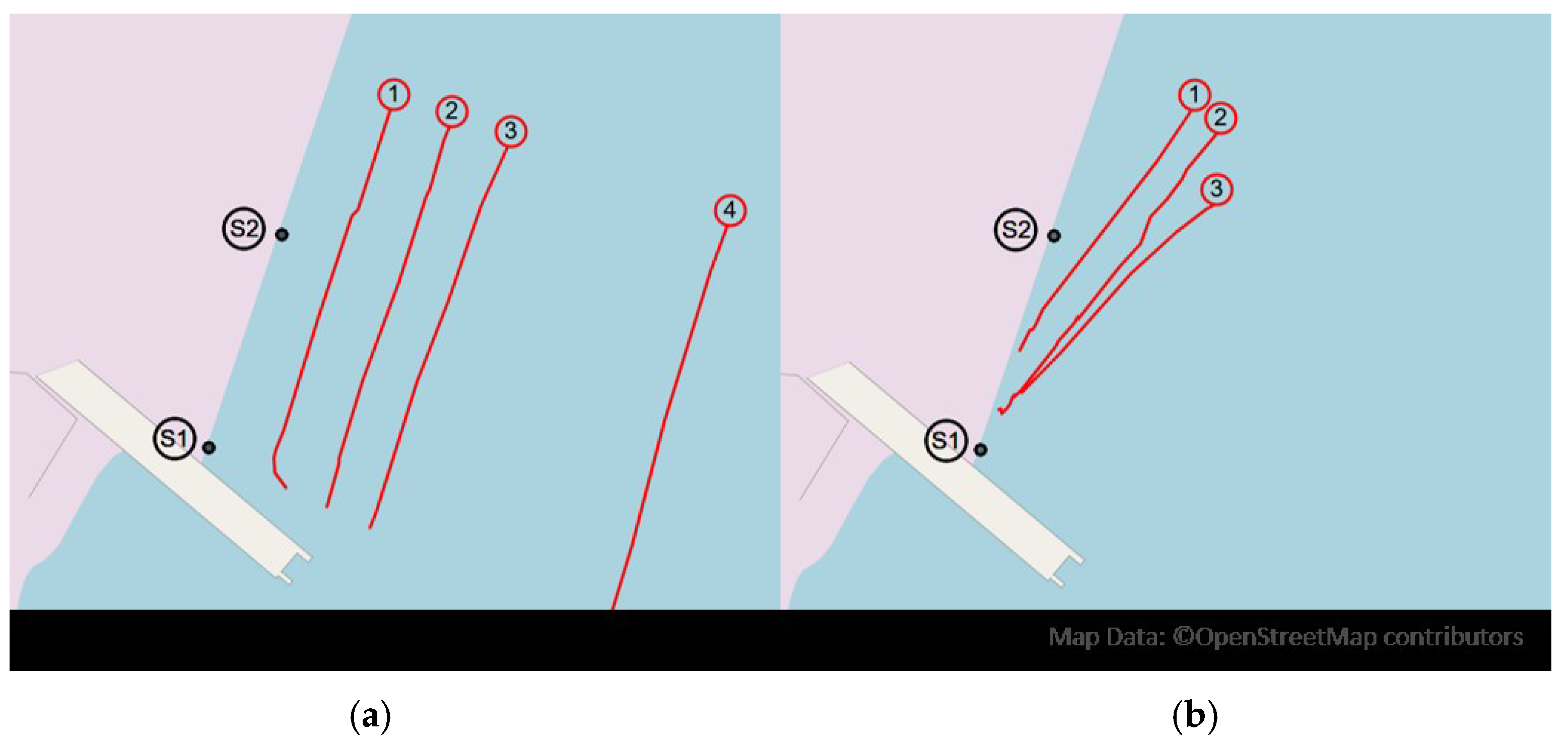
For the evaluation, we conducted a test campaign in Wilhelmshaven using the SmartKai prototype implementation and evaluated two types of maneuvers: parallel sailing along the quay and common regular berthing approaches as plotted by Figure 11.

Because vessels over 200 m approach with berthing angles < 0.5 degrees but the ship available for the test campaign was much smaller, we decided to sail parallel tracks in four different distances to the quay: 20 m, 40 m, 60 m, and 150 m. We did not consider closer distances as the detection range of the LD-LRS 3611 sensors started above 5 m and chose 150 m as the maximum distance based on weighting the requirements of the pilots that stated 120 m as the berthing initiation range with the technical characteristics of the LiDAR Sensors (we expected the best detection results until this distance even for bad weather situations). All these tracks had a similar length of around 125 m, were sailed with nearly 3 kn, and the track times were each between 92 and 98 s. For the 20 m parallel track, the vessel slowed down and initiated a turn towards the end of the track to avoid a collision with the adjacent quay wall. To have comparable parallel tracks, the 20 m track was therefore cut, starting from the point that the berthing angle was >5 degrees.

Moreover, three different berthing maneuvers were performed (c.f. Figure 11b). For berthing, the ship started north of our berthing location heading towards the quay. The ship is approaching the location with a berthing angle of 15 degrees and an initial speed of four knots and continuously reducing it to one knot. 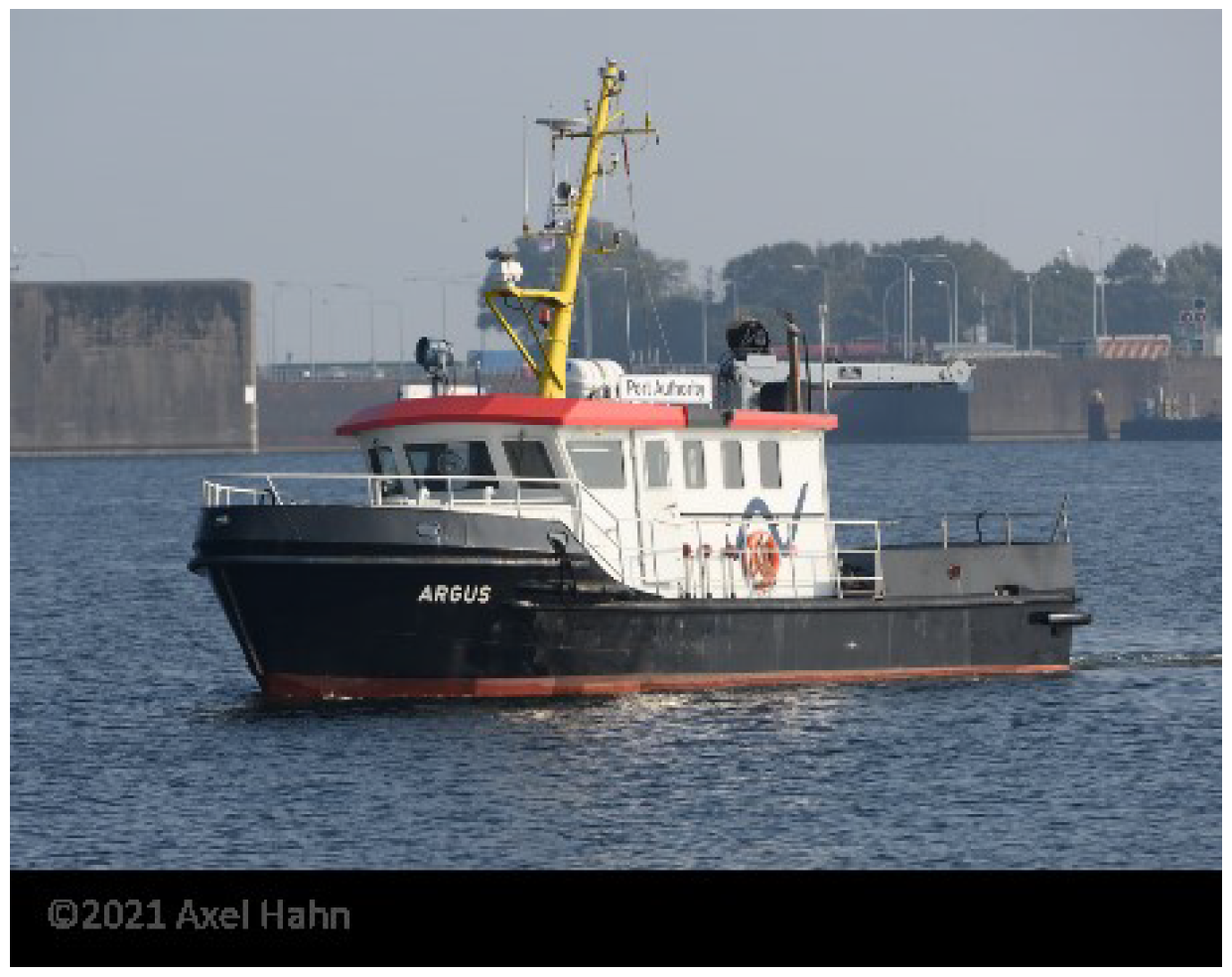A berthing angle of 15 degrees was the maximum of what was typically observed for smaller vessels without tug boat assistance [16], such as the Argus ship. The shipmaster’s target was to berth between the two LiDAR sensors. This scenario was also varied with a start speed of six knots. Because our LiDAR sensors have a minimum range of 5 m, they were clipped up to this distance. The track lengths vary between 38 and 54 s due to the different starting positions and velocities.

The Argus ship master performed all maneuvers by navigating manually with the help of the onboard bridge systems (ECIDS, compass, and GPS). For the experiment, we installed an additional IMO approved (transmitting heading and satellite navigation device) DGPS sensor (JRC JLR-21) centrally on the ship, which enabled us to record the sailed maneuver tracks with more precision and keep it in sync with the LiDAR sensor measurements. In our configuration, the sensor provides a minimum accuracy of 6 m by specification, which is less accurate than the LiDAR sensor. But there were no buildings or other infrastructure on the quay wall that could affect the DGPS measurements. Good weather conditions were also present during the test campaign. Without clouds, rain, or other influencing factors for the DGPS signal, and therefore with very good satellite coverage, we assume the DGPS fixes to be much more accurate and precise than the corresponding minima stated in the sensor specifications.

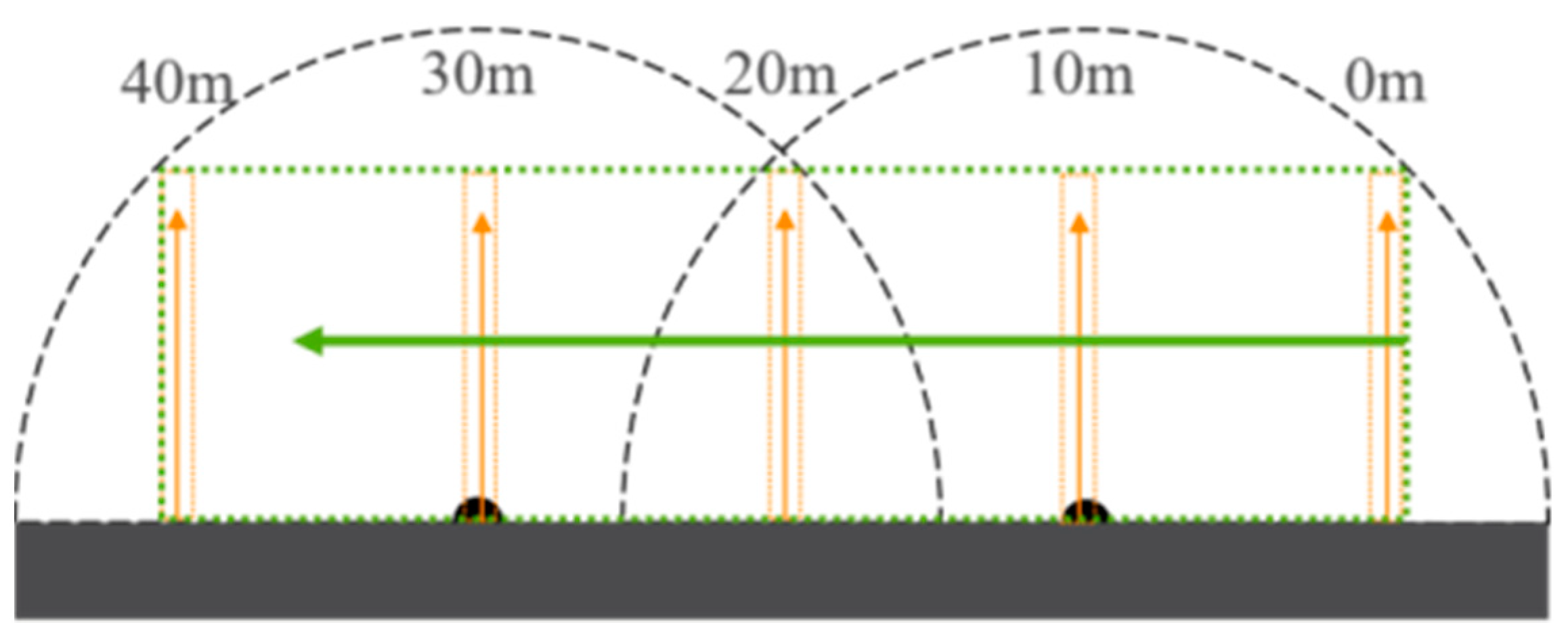
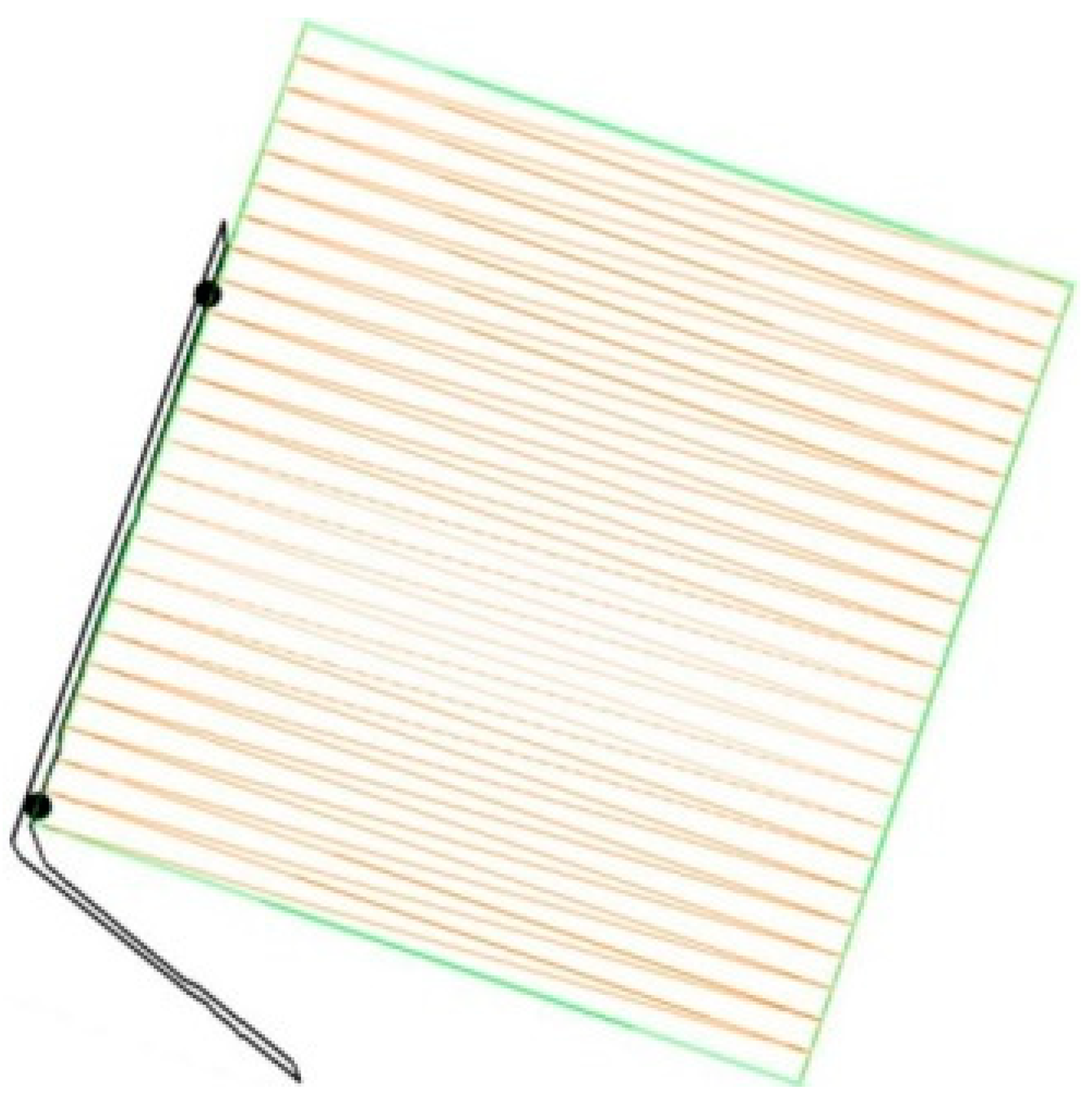
We defined Reference Points along the quay wall starting from the south-east sensor (c.f. Figure 9) every 5 m to reflect the Argus ship size for a total of 120 m resulting with 24 Reference Points. An additional Reference Point was placed at meter mark 0 m to indicate where the ship needs to stop. We also aligned a vertical one to the southern quay to communicate forward speed and distance from there as well. The length of the vertical Reference Points was increased to 150 m to cover the 150 m maneuver track. The same applies to the width of our horizontal Reference Point.

The following Section 6.2 covers the results of the parallel sailing maneuvers, whereas Section 6.3 focuses on presenting the results of the berthing scenarios with higher berthing angles.

6.2. Parallel Sailing Results

For the parallel tracks a maximum variance by half the width of the ship can be expected. This is because when entering the area of a Reference Point, the bow of the ship is detected first, followed by a gradual inclusion of the outer hull of the ship. Therefore, for the ship used for this paper, the expected maximum variance is 2.4 m.

Figure 12 depicts the four parallel scenarios and for the three sensor combinations the 95% interval together with the expected maximum variance of 2.4 m for the measured distances for each Reference Point (x-axis, numbered vertical Reference Points with 5 m spacing).

It can be seen that almost all measurements are within the expected variance, and also that with increasing distance the measurements fluctuate less. This can be explained by the higher point density especially at close ranges and the resulting better resolution of the bow. At higher distances, effects such as the lower point density and widening of the beam for better detection of the outer hull have to be considered.

Considering a Reference Point spacing of 5 m and a parallel sailing ship of 16 m length, on average 3.2 adjacent Reference Points are expected to communicate simultaneously a parallel sailing ship in 20 m, 40 m, 60 m, and 150 m.

Table 3. Number of Reference Points that detect a vessel simultaneously.

Scenario	Mean	STD
1.1 (20 m)	3.72	0.54
1.2 (40 m)	3.56	0.54
1.3 (60 m)	3.34	0.53
1.4 (150 m)	2.42	0.49

shows the mean and standard deviation divided according to the parallel runs. Here, the entry and exit times were removed so that the ship is completely inside the BSA.

For the first three scenarios with minor distances, the average is above the expected number of 3.2. In the 150 m scenario the ship sails outside the calculated BSA that requires at least three simultaneous measuring Reference Points. A significant reduction of the mean of measuring Reference Points for the 150 m scenario confirms the expectation. The standard deviation is around 0.5 for all scenarios. With increasing distance to the quay wall, the number of Reference Points that simultaneously detect a ship is reduced nearly linearly. Based on the calculations, we can also conclude that three reference points per ship length cannot be achieved in the 60 m scenario due to the standard deviation. In the initial sailing phase of the scenario, only the bow of the ship is detected. After the ship has passed the second sensor, the stern is also illuminated so that three Reference Points detect the ship. The illumination is therefore dependent on the relative positioning of the ship to the sensors. However, it is necessary to investigate why the average within the BSA is above the expected value of three. 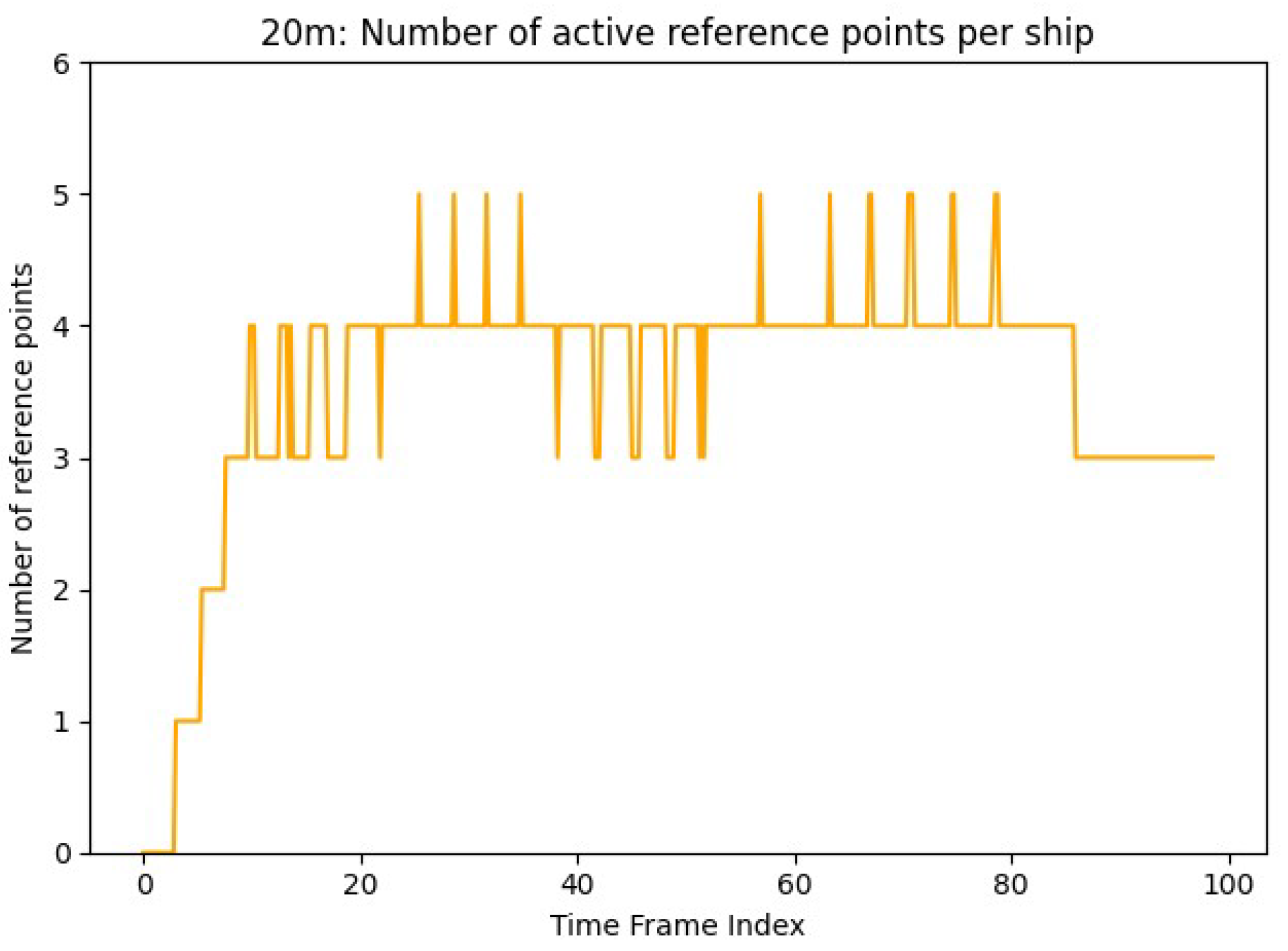Figure 13 shows for each timestamp the number of Reference Points that simultaneously detect a ship for the 20 m scenario including the entry and exit times.

In the first few seconds the ship enters the BSA, the number increases. As soon as the ship has completely entered the BSA, at least three Reference Points are able to measure the ship (after 16 s). It is noticeable that in short time intervals the number of Reference Points which recognize a ship briefly sinks or rises (example: between 60 s and 80 s). In these moments the ship leaves one Reference Point and changes to the next one, so that the number changes. The fact that the number is above the expected value of three is therefore due to the fact that with a 16 m ship length divided by 5 m a surplus arises. If the ship is seen by three Reference Points, the bow and stern can be in the adjacent Reference Points so that it is seen by five.

In addition to the number of active Reference Points, we also measured how often these were turned on and off. One would expect a ship to enter and exit each vertical Reference Point just once. A higher toggling number is an indicator that point outliers may occur, which would result in causing false alarms. We therefore measured how often a Reference Point is triggered, which is listed by

Table 4. Number of activations per Reference Point.

Scenario	Mean	STD	Max
1.1 (20 m)	1.16	0.46	3
1.2 (40 m)	1.12	0.32	2
1.3 (60 m)	1.12	0.32	2
1.4 (150 m)	1.32	0.61	3

.

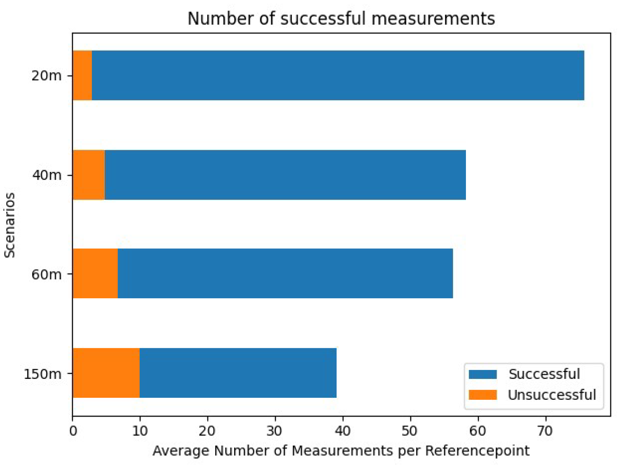
For none of the scenarios the expected value of one activation per scenario was reached. For the 20 m and the 150 m scenario a Reference Point was activated three times. In the 20 m scenario this was caused by point outliers caused by the relatively tiny hull size of the ship. Due to the fact that 2D LiDAR sensors were used, movements of the ship on the X or Z axis result in suddenly seeing other parts than the hull such as objects on the ship’s deck. For the 150 m scenario, we realized that the point density of the ship is significantly lower than for the other scenarios. Due to the minimum number of points that must lie within a Reference Point in order to perform a distance measurement, measurements are discarded more often, and thus false alarms are produced more frequently. We therefore checked how often measurements were discarded. For this purpose, we collected the number of successful and unsuccessful measurements. Successful in this context means that there are at least five points per Reference Point measurement. Otherwise, measurements are not successful and were not considered. Figure 14 summarizes the number of successful and unsuccessful measurements for each scenario.

We recognized that with higher distance the point density decreases, and the number of unsuccessful measurements increases. Regarding the 150 m scenario, approximately 25% of our measurements were not considered because of the low point density. The still high amount of successful measurements indicates that the IMO positioning fix requirements of 1 Hz while berthing can be fulfilled with the 5 Hz sensor. To investigate this in more detail, we measured how many times per second a Reference Point takes a measurement. The factors that influence the calculation rate are the time synchronization of the LiDAR measurement and the failure rate due to too few points. Figure 15 shows the calculated average Hz number for each scenario.

Due to the refresh rate of the sensor, the upper limit is 5 Hz, and our results are very close to this value. However, it is noticeable that there are a few outliers. The lowest value can be observed for the 150 m scenario (4.2 Hz).

6.3. Berthing Maneuvers Results

Scenarios 2.1–2.3 define the other extreme of berthing maneuvers with an angle of 15 degrees (which is in fact a typical berthing angle for small ships such as the one we used for our experiments). We evaluated the distance to Reference Point, speed, forward speed, and distance to meter mark 0 m. For these metrics, we examined the deviations from the DGPS. Because in general we expected the accuracy and precision of the DGPS to be much lower when compared to LiDAR, we focused a comparison of the measurement deviations to verify the stability of the Reference Point measurements.

We will start with the comparison of the measured distances on vertical (distance to the quay wall) and horizontal (distance ahead) level. It is expected that the variance of the measurements is low and thus a constant deviation between both measurement methods is achieved. Because several Reference Points were defined along the quay wall, but a DGPS sensor only determines a single position and speed, the measurements of the Reference Points are combined. Therefore, the shortest distance of all Reference Points is used as a reference value to compare it with the DGPS. Based on the determined positions of the GPS sensor, we calculated the vertical distance to the quay wall and the horizontal distance to enable the comparison.

Figure 16 shows the vertical (a) and horizontal (b) deviations between the Reference Point measurements and the DGPS.

In scenario 2.1, the variance of the measurements is small compared to other scenarios. However, with respect to the horizontal distance measurements, outliers are present. In the second scenario (2.2), the highest variance is present. Accordingly, the minimum and maximum values are also high. Due to the high range of values, there are also no outliers. In the third scenario, the variance is similar to that of scenario 2.1 (vertical and horizontal). However, outliers are also found here, especially below the minimum value. To first check for outliers in the first scenario, we first examine the horizontal distance measurements.

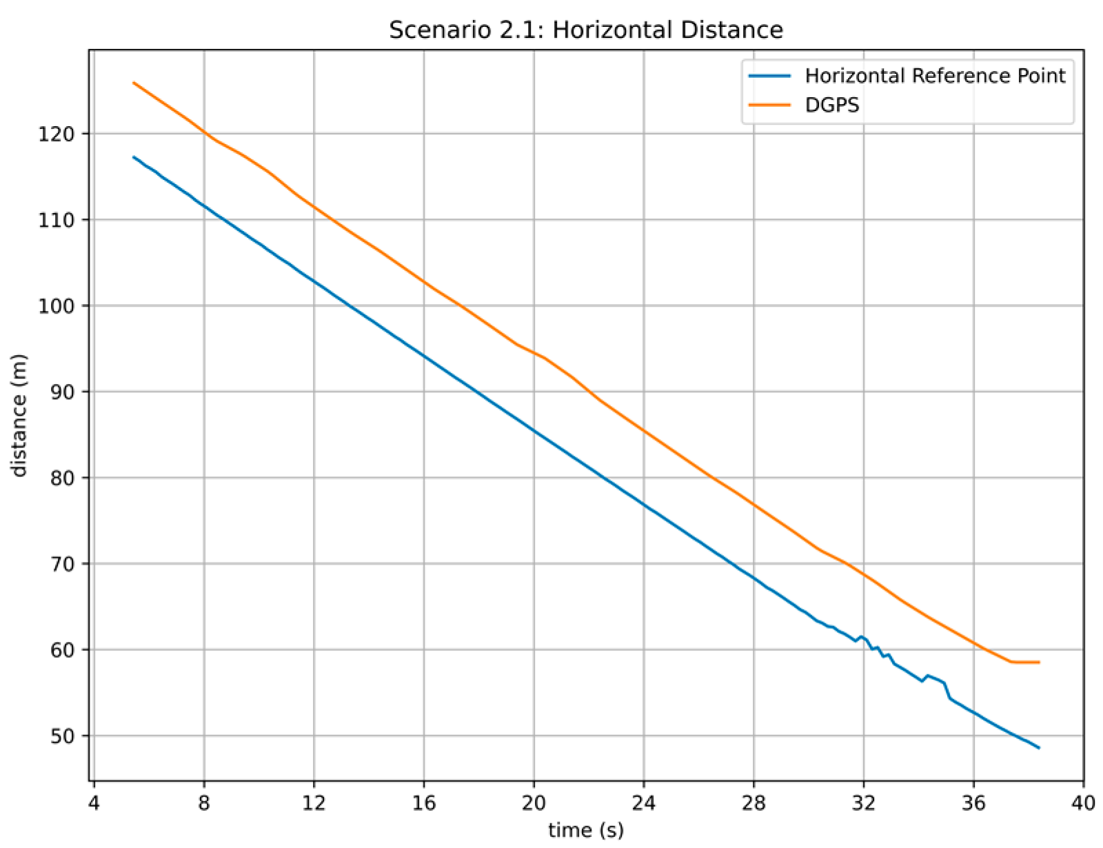
Figure 17 shows the horizontal distance measurements to the quay wall for scenario 2.1.

Up to second 32, the deviations between the measurement methods are relatively constant. From this point on, however, the horizontal Reference Point shows fluctuating distance measurements, which causes the outliers in Figure 16b. Regardless of the scenario considered, these anomalies are also found in other scenarios (cf. Figure 16 scenario 2.3), although we ascertained that the length of these phases is smaller.

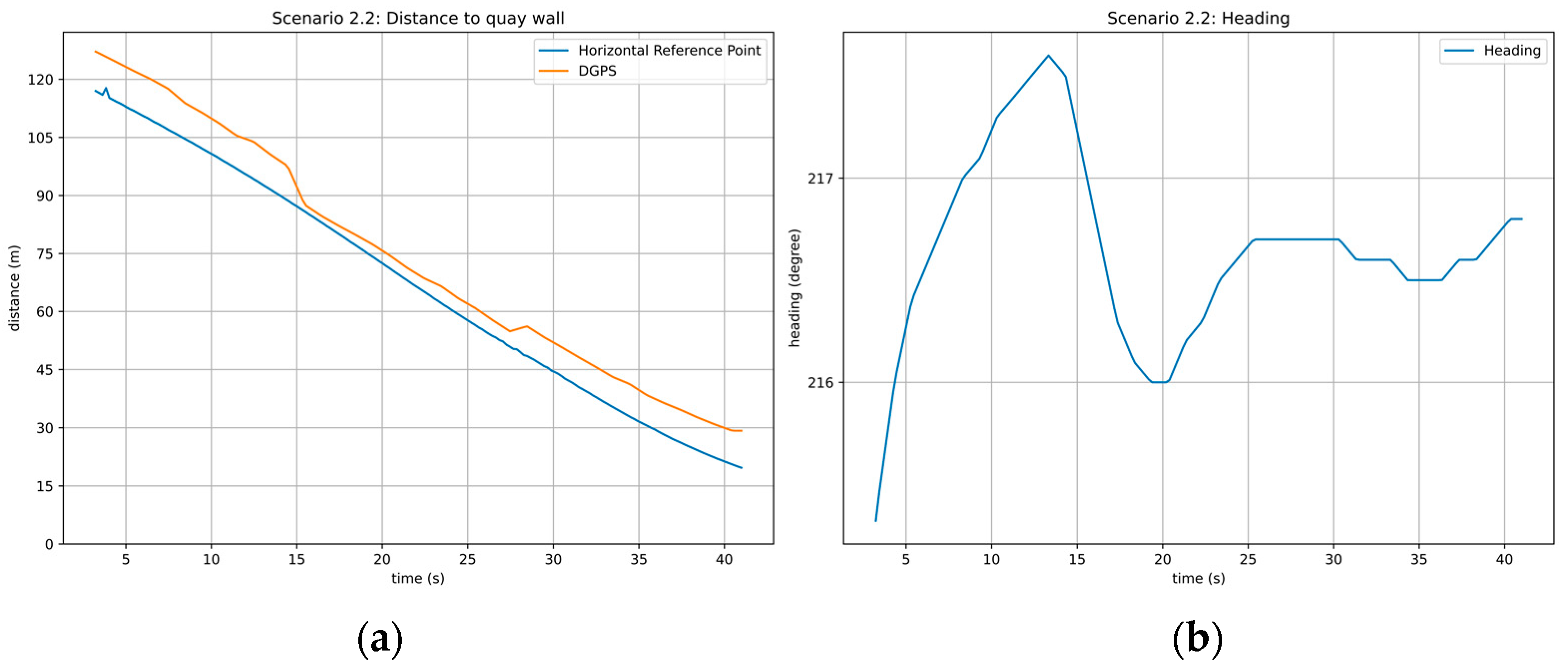
The next step is to investigate the high variance in scenario 2.2. For this purpose, Figure 18 shows the horizontal distance to the quay wall (a) and the heading of the ship (b).

It is particularly striking that the deviations between the two measurement methods decrease between 15 s and 27 s. This increases the variance of the measurements, which is reflected in the Figure 16b. However, the reason for this behavior is unknown. As can be seen from the right side of the figure, the ship did not change course. In the period under consideration, only a course change of <1° was made. We also checked the quality of the DGPS measurements. However, the number of satellites was constant at 8 and the Horizontal Dilution of precision (HDOP) was 1. Infrastructure at the mooring was not available, so the GPS measurements were not exposed to any influence. We therefore assume that this is an anomaly.

The next part is the comparison of measured speed between Reference Points and DGPS. For these we examine the average, standard deviation, mean error, and rooted mean squared error (RMSE) to be able to make a statement about the stability of the measurements. Due to deviations in the distance measurements (see Figure 16), we have removed all speed values greater than 10 m/s, as this leads to disproportionate deviations. However, they will be analyzed in more detail in the following.

Table 5. Comparison of vertical approach speed between Reference Points approach and DGPS measurements using berthing scenarios (Scenarios 2.1–2.3).

	Reference Points		DGPS		Deviations
Scenario	Mean	STD	Mean	STD	Mean Error	RMSE
2.1	0.68 m/s	0.11 m/s	0.66 m/s	0.1 m/s	−0.01	0.11
2.2	0.89 m/s	0.19 m/s	0.83 m/s	0.19 m/s	−0.07	0.21
2.3	0.81 m/s	0.15 m/s	0.8 m/s	0.09 m/s	−0.01	0.14

shows the vertical velocity measurements (quay wall approach speed) of the respective scenarios.

The table shows that the measurements of the two methods are quite comparable. In all scenarios the absolute deviation is below 0.07 m/s (peak in Scenario 2.2). The highest deviation was recorded in scenario 2.2, in which the position anomalies on Figure 18 cause varying velocity anomalies to be measured. However, the standard deviation of the Reference Points is consistently higher than that of the DGPS, so that the measurements vary more strongly. Due to the higher measurement rate of the LiDAR sensors (5 Hz) compared to the DGPS (1 Hz), more velocity measurements were recorded, which led to higher deviations.

Table 6. Comparison of forward speed between Reference Points approach and DGPS measurements using berthing scenarios (Scenarios 2.1–2.3).

	Reference Points		DGPS		Deviations
Scenario	Mean	STD	Mean	STD	Mean Error	RMSE
2.1	2.09 m/s	0.98 m/s	2.08 m/s	0.25 m/s	−0.01	0.99
2.2	2.52 m/s	0.95 m/s	2.59 m/s	1.21 m/s	0.08	1.44
2.3	1.59 m/s	0.7 m/s	1.6 m/s	0.34 m/s	0.01	0.63

shows the measured forward velocities of the horizontal Reference Point and the DGPS.

Again, the absolute deviation to the DGPS is relatively small and is below 0.08 (peak again in scenario 2.2). Again, however, the standard deviation of the Reference Points is higher in scenario 2.1 and 2.3 than for the DGPS. Especially in scenario 2.3, the standard deviation is two times higher.

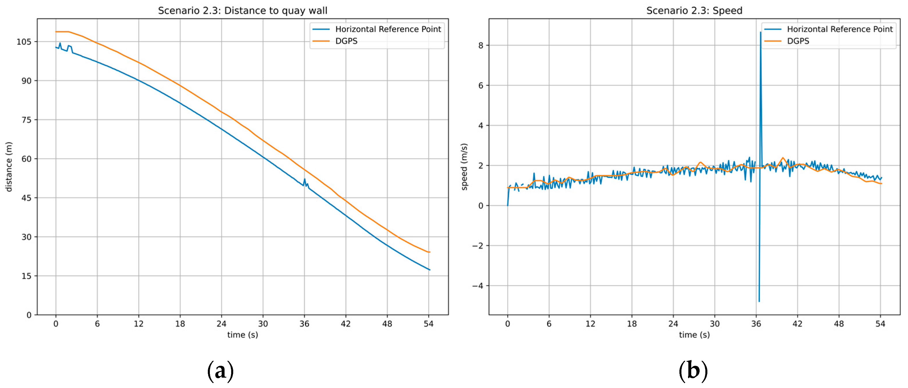
The highest speed deviation between both systems was recorded for scenario 2.3 (peak deviation). We also observed a high standard deviation for the Reference Points in this scenario, compared to DGPS. Because the velocity is calculated based on the measured distance, we further investigated in the distance measurements of scenario 2.3. Figure 19 depicts the distance to meter mark 0 m and the resulting forward speed of the vessel.

We observed that the deviation in distance between the DGPS sensor and the horizontal Reference Point is relatively constant between 5 and 8 m apart (cf. Figure 16b). However, between second 0 and 3 we measured jitter in the horizontal distance to meter mark 0 m. Because this generates incomparably high-speed measurements, they were removed. Velocity anomalies were also measured in the time range between 35 and 37. This results in speed deviations; thus, we calculated a maximum above ~8 m/s and a minimum below ~−4 m/s in forward speed. Due to the high update frequency of the LiDAR sensor (5 Hz) and distance change in a small time-window, the resulting forward speed is high. Compared to the DGPS, we can see that the reference points take varying velocity measurements, thus resulting in jitter. In comparison to the DGPS sensor, less frequent speed changes can be observed. High-speed deviations were also observed for the other scenarios. Therefore, to improve the stability of the measurements, a filter is required to smoothen the speed measurements for the nautical personnel.

7. Discussion

After considering the results of the previous section, it appears that the concept of Reference Points is promising. We applied the Reference Point method to four parallel and three berthing tracks with the port operation ship Argus and specifically focused on the corner cases (very small berthing and very high berthing angles).

Our setup is based on defining at least three Reference Points per ship length to ensure that a future system could also calculate berthing angles and rate of turn (ROT) based on the Reference Points. We showed that this can be ensured as long as the ship is within the specified sensor range. As soon as the ship is outside the BSA (for the 150 m scenario) and thus outside the specifications, only two reference points could simultaneously detect the ship. Running with 5 Hz, the IMO requirements that require 1 Hz fixations can be easily achieved (we reported at least 4.2 Hz with an average close to the maximum refresh rate of 5 Hz). Verification of the spread of measurements showed that almost all measurements at all reference points were within the range that we anticipated.

The comparison between LiDAR and GPS showed that deviations were within the expected range of half a ship width (with the GPS antenna assumed to be installed at the center of the ship). Nearly all of the deviations can be explained by a dependence on the heading, because the ship’s hull is longer than it is wide and the LiDAR sensors detect the hull of the ship while the GPS measures the position at the ship-center. Thus, a change of the orientation has no effect on the GPS measurement, but directly one on the measured minimum distance via LiDAR.

Furthermore, when looking at the results, it is noticeable that many of the errors mentioned above occurred during fluctuations of the LiDAR measurements and thus individual measured values led to outliers. This can be explained to a large extent by the prototypical design of the system, where the LiDAR was positioned a little too high. It can be seen on the picture of the ship (Figure 7) that the shape of the hull in the middle of the side does not reach the same height as at the bow and stern of the ship. If the ship is now positioned unfavorably to the sensor, it is therefore possible that the hull was not ideally hit and thus the structure of the ship is briefly measured. Therefore, to improve detection for smaller ships, 3D LiDAR sensors must be applied. This would make it possible to reduce the outliers, because measurements are not only made on the horizontal plane. For bigger vessels (which are actually the targeted ones), these kind of LiDAR fluctuations would not be expected.

Regardless of the point measurement errors, it remains a problem to use the sensor values directly to determine the speed. Our velocity measurements have shown a high standard deviation and the reliability of these are therefore low. Due to the high frequency of the LiDAR sensors, small distance deviations provide high speeds. Therefore, these must be filtered before they are used. Assuming that the reason for the deviations is the frequency of the measurements, we decided to calculate them only once per second (1 Hz) to compensate for the fluctuations. Figure 20 plots the horizontal speed calculation for scenario 2.3.

The DGPS measures velocity in 1 Hz intervals, with measurements based on LiDAR in 5 Hz (sensor specification) and in 1 Hz. The calculation in 5 Hz intervals shows high fluctuations compared to the DGPS. But if the velocity is calculated only once per second, the fluctuations are massively reduced. Only between second 34 and 37 are high deviations found in the LiDAR data, so that outliers are generated. However, these outliers are much lower than previous measurements. To further investigate the performance of these methods,

Table 7. Comparison of speed filtering methods.

Method	Mean	STD	RMSE
DGPS	1.6	0.34	-
LiDAR 5 Hz	1.59	0.7	0.63
LiDAR 1 Hz	1.6	0.34	0.17

shows the mean, standard deviation, and RMSE compared to the DGPS of all methods.

If the speed measurement is performed only once per second, the deviations are close to those of the DGPS and reduce the RMSE from 0.63 to 0.17. The precision and accuracy of the used DGPS sensor is not a sufficient ground truth for evaluating the LiDAR sensor to validate the accuracy of the velocity measurements. However, a reduction in fluctuations would lead to better stability to present more consistent measurements to nautical personnel. Nevertheless, because we do not have ground truth, it is also possible that more accurate velocity values were obtained from the LiDAR measurements. Future work should therefore select appropriate filtering techniques and collect ground truth measurements to validate the calculations.

Another point we noticed during the evaluation is that it is relatively difficult to evaluate LiDAR-based methods. Because these sensors can have high accuracy down to the millimeter range, only a few comparable sensors can be found. Therefore, better evaluation sensor technology must be used for ground truth measurements. It is also difficult to evaluate the robustness and reliability of the system. LiDAR-based techniques are dependent on various weather conditions, so long term testing is required. Alternatively, realistic ship and sensor simulations must be used to test all possible situations.

8. Conclusions

In this paper, we presented a ship-independent mooring assistance system based on LiDAR sensors. For this, we summarized interviews performed with pilots in the form of workshops and derived requirements for our proposed BAS. Then we presented the current state in shore-based assistant systems and checked if these can cover all of the pilots’ requirements that we ascertained. We found that most systems make use of non-deterministic or black box algorithms, so that the functional safety is hard to ensure. We have therefore introduced the concept of a Reference Point. They can be arbitrarily placed on a mooring site e.g., to reflect typical landmarks that pilots typically used for orientation to during berthing. We have placed vertical Reference Points along the quay wall to measure the distance to the quay wall and the approach speed. Horizontal Reference Points are placed at the end of the berth to measure the approach distance and speed. To ensure functional safety, we defined a Berthing Support Area based on the port structure, sensor specifications, and pilotage requirements. The BSA was determined by a mathematical model and defines an area in which the support is provided by calculating the possible illumination of a target by LiDAR sensors.

We implemented the BSA within the SmartKai project and installed the system at a berth in Wilhelmshaven in Germany. For the evaluation of our BAS, we conducted a test campaign using this prototypical setup. We performed several scenarios (parallel sailing and berthing scenarios) to verify that our BAS conforms with the requirements derived based on pilot interviews. Our results show that we can fulfill most of our requirements. The BAS conforms to the IMO Resolution A.915 (22) with respect to the required update frequency of 4.2 Hz > 1 Hz. We were able to achieve a high measurement stability, in which only a few outliers could be found. Accuracy measurements require further investigations with more accurate sensors than the applied DGPS sensors. We observed that the biggest challenge for our system is the speed calculation. Because of the high update frequency of the LiDAR sensors, small distance deviations result in high-speed deviations. Thus, an approach is needed to filter the distance measurements beforehand to retrieve accurate speed calculations.

With the concept of Reference Points and the Berthing Support Area, we see additional use cases that can be covered. In the future, we want to support pilots not only during berthing maneuvers, but also during casting off. In situations involving tug assistance, such a system could also offer important data not only to the captain of the vessel but also to the skippers of the tugs, improving the coordination between vessel and tugboats. In our interviews, the pilots have reported that not only the distance to the quay wall, but also the rate of turn of a ship is an important information. Thus, using multiple Reference Points, the heading of a ship and the rate of turn could be determined. Warnings, for example, at high approach speeds or high rate of turns could also provide additional support. Therefore, captains and pilots should be warned about a possible danger to improve the safety of the berthing process. Further use cases include support during approaching lock entrances or bridge crossings. The BSA can additionally be transferred to other LiDAR-based systems.

Furthermore, it is also possible to integrate our system into Berthing Planning Systems [36]. Compared to other systems, Reference Points are only loosely coupled with each other. Therefore, our system can be dynamically split if needed (e.g., dividing one berth into several), so that this flexibility supports harbor operators in the dynamic environment of the port. This is especially useful for unintended berths, where berth locations are dynamically allocated [37]. This approach can also support the planning of berthing processes in the port. In [24] and [25], procedures were presented to solve the berth allocation and quay crane assignment problem. The authors partition the berth into segments and assign a slot to arriving vessels. This procedure can be supported by partitioning the reference points to ensure a safe and efficient berthing process.

References

1. Sánchez, R.J.; Perrotti, D.E.; Fort, A.G.P. Looking into the Future Ten Years Later: Big Full Containerships and Their Arrival to South American Ports. J. Shipp. Trade 2021, 6, 2. [Google Scholar] [CrossRef]
2. Forum, I.T. The Impact of Mega-Ships; International Transport Forum Policy Papers, No. 10; OECD Publishing: Paris, France, 2015. [Google Scholar] [CrossRef]
3. Sánchez, R.; Mouftier, L. Reflections on the Future of Ports: From Current Strains to the Changes and Innovation of the Future; CEPAL: Santiago, Chile, 2016. [Google Scholar]
4. Hsu, W.-K.K. Assessing the Safety Factors of Ship Berthing Operations. J. Navig. 2015, 68, 576–588. [Google Scholar] [CrossRef] [Green Version]
5. Bui, V.; Kawai, H.; Kim, Y.-B.; Lee, K. A Ship Berthing System Design with Four Tug Boats. J. Mech. Sci. Technol. 2011, 25, 1257–1264. [Google Scholar] [CrossRef]
6. Felski, A.; Naus, K.; Świerczyński, S.; Wąż, M.; Zwolan, P. Present Status And Tendencies In Docking Systems’ Development. Annu. Navig. 2014, 21. [Google Scholar] [CrossRef] [Green Version]
7. Harati-Mokhtari, A.; Wall, A.; Brooks, P.; Wang, J. Automatic Identification System (AIS): Data Reliability and Human Error Implications. J. Navig. 2007, 60, 373–389. [Google Scholar] [CrossRef]
8. Bialer, O.; Jonas, A.; Tirer, T. Super Resolution Wide Aperture Automotive Radar. IEEE Sens. J. 2021, 21, 17846–17858. [Google Scholar] [CrossRef]
9. Athavale, R.; Ram, D.S.H.; Nair, B. Low Cost Solution for 3D Mapping of Environment Using 1D LIDAR for Autonomous Navigation. In IOP Conference Series: Materials Science and Engineering; IOP Publishing: Bristol, UK, 2019; Volume 561, p. 012104. [Google Scholar] [CrossRef] [Green Version]
10. Trelleborg Smart Dock Laser. Available online: https://www.trelleborg.com/en/marine-and-infrastructure/products-solutions-and-services/marine/docking-and-mooring/docking-aid-system/smart-dock-laser (accessed on 17 February 2021).
11. DockAssist®. The Most Advanced Berthing Aid System in the World; Metratek Telematics Ltd.: Nicosia, Cyprus; Available online: https://metratek.co.uk/dockassist (accessed on 10 February 2021).
12. Reiher, D.; Hahn, A. Review on the Current State of Scenario-and Simulation-Based V&V in Application for Maritime Traffic Systems; IEEE: Piscataway, NJ, USA, 2021. [Google Scholar]
13. Corso, A.; Moss, R.J.; Koren, M.; Lee, R.; Kochenderfer, M.J. A Survey of Algorithms for Black-Box Safety Validation. J. Artif. Intell. Res. 2021. [Google Scholar] [CrossRef]
14. Czarnecki, K. Operational Design Domain for Automated Driving Systems—Taxonomy of Basic Terms; Waterloo Intelligent Systems Engineering (WISE) Lab.: Waterloo, ON, Canada, 2018. [Google Scholar]
15. Falk, M.; Saager, M.; Harre, M.-C.; Feuerstack, S. Augmented berthing support for maritime pilots using a shore-based sensor infrastructure. In HCI International 2020—Late Breaking Posters; Communications in Computer and Information, Science; Stephanidis, C., Antona, M., Ntoa, S., Eds.; Springer International Publishing: Cham, Switzerland, 2020; Volume 1294, pp. 553–559. ISBN 978-3-030-60702-9. [Google Scholar]
16. PIANC—International Navigation Association. Guidelines for the Design of Fender Systems—MarCom Report of WG 33. 2002. Available online: https://www.pianc.org/publications/marcom/guidelines-for-the-design-of-fender-systems (accessed on 1 February 2021).
17. Hein, C. Anlegegeschwindigkeiten von Großcontainerschiffen. In Proceedings of the PIANC Deutschland (Hg.): Deutsche Beiträge, 33. Internationaler Schifffahrtskongreß, San Francisco, CA, USA, 1–5 June 2014; PIANC Deutschland: Bonn, Germany, 2014; pp. 1–5. [Google Scholar]
18. Stadt Wilhelmshaven Besondere Hafenordnung Für Den Stadthafen Wilhelmshaven. Available online: https://www.wilhelmshaven.de/PDF/Stadtrecht/Sr32-09_Besondere_Hafenordnung_fuer_den_Stadthafen_WHV.pdf?m=1418987622& (accessed on 23 August 2021).
19. IMO Resolution, A. 915 (22) Revised Maritime Policy and Requirements for a Future Global Navigation Satellite System (GNSS); Adopted on 29 November 2001; International Maritime Organization: London, UK, 2001. [Google Scholar]
20. Perkovič, M.; Gucma, L.; Bilewski, M.; Muczynski, B.; Dimc, F.; Luin, B.; Vidmar, P.; Lorenčič, V.; Batista, M. Laser-Based Aid Systems for Berthing and Docking. J. Mar. Sci. Eng. 2020, 8, 346. [Google Scholar] [CrossRef]
21. Kim, H.; Kim, D.; Park, B.; Lee, S.-M. Artificial Intelligence Vision-Based Monitoring System for Ship Berthing. IEEE Access 2020, 8, 227014–227023. [Google Scholar] [CrossRef]
22. Chen, C.; Li, Y. Ship Berthing Information Extraction System Using Three-Dimensional Light Detection and Ranging Data. J. Mar. Sci. Eng. 2021, 9, 747. [Google Scholar] [CrossRef]
23. Kuzu, A.; Arslan, O. Analytic comparison of different mooring systems. In Proceedings of the Global Perspectives in MET: Towards Suistainable, Green and Integrated Maritime Transport, Varna, Bulgaria, 11–14 October 2017. [Google Scholar]
24. Iris, Ç.; Pacino, D.; Ropke, S.; Larsen, A. Integrated Berth Allocation and Quay Crane Assignment Problem: Set Partitioning Models and Computational Results. Transp. Res. Part E Logist. Transp. Rev. 2015, 81, 75–97. [Google Scholar] [CrossRef] [Green Version]
25. Iris, Ç.; Lam, J.S.L. Recoverable Robustness in Weekly Berth and Quay Crane Planning. Transp. Res. Part B Methodol. 2019, 122, 365–389. [Google Scholar] [CrossRef]
26. Iris, Ç.; Lam, J.S.L. A Review of Energy Efficiency in Ports: Operational Strategies, Technologies and Energy Management Systems. Renew. Sustain. Energy Rev. 2019, 112, 170–182. [Google Scholar] [CrossRef]
27. Automated Mooring. Available online: https://www.cavotec.com/en/your-applications/ports-maritime/automated-mooring (accessed on 21 January 2022).
28. AutoMoor—Automated Mooring System. Available online: http://www.trelleborg.com/en/marine-and-infrastructure/resources/videos/automoor-automated-mooring-system (accessed on 21 January 2022).
29. In Tallinn Old City Harbour Ships Are Now Served by Automated Mooring Equipment. Port of Tallinn. 2021. Available online: https://www.ts.ee/en/in-tallinn-old-city-harbour-ships-are-now-served-by-automated-mooring-equipment/ (accessed on 17 January 2022).
30. Fischer, Y. Wissensbasierte Probabilistische Modellierung für die Situationsanalyse am Beispiel der Maritimen Überwachung. Available online: https://publikationen.bibliothek.kit.edu/1000051065 (accessed on 5 February 2022).
31. Rossmann, J.; Schluse, M.; Bücken, A.; Krahwinkler, P. Using airborne laser-scanner-data in forestry management: A novel approach to single tree delineation. In Proceedings of the ISPRS Workshop on Laser Scanning, Espoo, Finland, 12–14 September 2007. [Google Scholar]
32. SmartKai—EMIR. Available online: https://www.emaritime.de/smartkai/ (accessed on 29 October 2021).
33. Goodin, C.; Carruth, D.; Doude, M.; Hudson, C. Predicting the Influence of Rain on LIDAR in ADAS. Electronics 2019, 8, 89. [Google Scholar] [CrossRef] [Green Version]
34. Montalban, K.; Reymann, C.; Atchuthan, D.; Dupouy, P.; Rivière, N.; Lacroix, S. A Quantitative Analysis of Point Clouds from Automotive Lidars Exposed to Artificial Rain and Fog. Atmosphere 2021, 12, 738. [Google Scholar] [CrossRef]
35. Stanley, M.; Laefer, D. Metrics for Aerial, Urban Lidar Point Clouds. ISPRS J. Photogramm. Remote Sens. 2021, 175, 268–281. [Google Scholar] [CrossRef]
36. Dai, J.; Lin, W.; Moorthy, R.; Teo, C.-P. Berth Allocation Planning Optimization in Container Terminals. In Supply Chain Analysis; Tang, C.S., Teo, C.-P., Wei, K.-K., Eds.; International Series in Operations Research & Mana; Springer: Boston, MA, USA, 2008; Volume 119, pp. 69–104. ISBN 978-0-387-75239-6. [Google Scholar]
37. Imai, A.; Nishimura, E.; Hattori, M.; Papadimitriou, S. Berth Allocation at Indented Berths for Mega-Containerships. Eur. J. Oper. Res. 2007, 179, 579–593. [Google Scholar] [CrossRef] [Green Version]
Figure 1. Analysis based on interviews with harbor and river pilots taken and adapted from [15].
Jmse 10 00385 g001
Figure 2. Concept of a Reference Point. Origin p is the point to which the distance of a vessel is calculated. A filter box is marked by dotted lines, which is defined by a length l and a width w. Starting from the point, the perpendicular distance to a ship is calculated, which is marked by a point cloud (black dots).
Jmse 10 00385 g002
Figure 3. Berthing Assistant System Concept. LiDAR sensor positions shown as dots and their detection range in semi circles. Vertical Reference Points measure the distance in relation to quay wall. Horizontal Reference Points shown in green measure the distance to meter mark zero.
Jmse 10 00385 g003
Figure 4. The BSA derivation and operation process. The former one includes set setup and validation to gain Reference Points, while the latter summarizes the process for the Reference Points to be used to determine the distance and speed measurements.
Jmse 10 00385 g004
Figure 5. (a) Prototype implementation of SmartKai in the port of Wilhelmshaven, Germany. Red dots mark the position of two 2D LiDAR sensors. (b) Resulting LiDAR data from 2D LiDARs installed at the quay wall. Quay wall outline and a ship on the right image can clearly be seen.
Jmse 10 00385 g005
Figure 6. Sensor processing unit with battery backup that records the data from the LiDAR sensors together with various other sensors, such as AIS, camera, and weather-related information, and also communicates processed information via the mobile network.
Jmse 10 00385 g006
Figure 7. NPorts Port operation ship ARGUS.
Jmse 10 00385 g007
Figure 8. (a) Relationship between sensor position, ship-angle, and section width. (b) Contour-map of the number of rays that hit a section surrounding each position on the map.
Jmse 10 00385 g008
Figure 9. Quay wall model extracted from a point cloud. Black dots show the position of the LiDAR sensors. Polygon on the left shows the extracted quay wall shape. Orange boxes show the location and box filter of the defined vertical Reference Point filters. Additional horizontal Reference Point is marked as green rectangle.
Jmse 10 00385 g009
Figure 10. (a) Raw LiDAR data transformed into a global coordinate system. In green: identified quay wall, red: static infrastructure removed from further processing. (b) resulting data after point cloud preprocessing. Quay wall points were replaced by the quay wall shape resulting from the world model.
Jmse 10 00385 g010
Figure 11. Test campaign scenarios (a) parallel sailing (scenarios 1.1–1.4), (b) berthing maneuvers (scenarios 2.1–2.3).
Jmse 10 00385 g011
Figure 12. Measured distances against the maximum allowed spread for each sensor and scenario configuration.
Jmse 10 00385 g012
Figure 13. Number of active Reference Points during the 20 m scenario.
Jmse 10 00385 g013
Figure 14. Number of successful and unsuccessful measurements of Reference Points. With a raising distance the number of successful measurements decreases.
Jmse 10 00385 g014
Figure 15. Average Hz of Reference Points per scenario.
Jmse 10 00385 g015
Figure 16. Vertical ((a), left) and horizontal ((b), right) deviations between DGPS sensor and Reference Points.
Jmse 10 00385 g016
Figure 17. Scenario 2.1 horizontal distance to quay wall.
Jmse 10 00385 g017
Figure 18. Scenario 2.2 horizontal distance to quay wall (a) and ships heading (b).
Jmse 10 00385 g018
Figure 19. Horizontal distance to meter mark 0 m (a) and forward speed for scenario 2.3 (b).
Jmse 10 00385 g019
Figure 20. Comparison of speed filtering methods for scenario 2.3.
Jmse 10 00385 g020