Working Performance of the Deep-Sea Valve-Controlled Hydraulic Cylinder System under Pressure-Dependent Viscosity Change and Hydrodynamic Effects

Abstract

The valve-controlled hydraulic cylinder system (VCHCS) is commonly used for actuators such as manipulators in deep-sea equipment, whose working performance is crucial to subsea tasks. Affected by the ambient pressure introduced by the pressure compensator, the viscosity of the hydraulic oil increases significantly. On this basis, the viscosity changes further when flowing in the slender pipeline, making the pipeline pressure loss substantially increase and subsequently affecting the working performance of the deep-sea VCHCS. Aiming at this issue, a detailed nonlinear mathematical model of the deep-sea VCHCS is established, in which the viscosity-pressure characteristics of the hydraulic oil is considered to take the viscosity changes in the pipeline into account. Besides, the hydrodynamic effects are also included in the model. Then the corresponding numerical simulation model of the deep-sea VCHCS is established, and its working performance at different depths is simulated and analyzed. When the depth is 11km, the extension and retraction movements are delayed by 52.50% and 43.12% respectively. The root cause of the delay is then analyzed and discussed. Finally, the parameters that affect the working performance are studied, and suggestions to reduce or eliminate the delay phenomenon are given. The results can provide theoretical support for the performance optimization of the deep-sea VCHCS.

1. Introduction

For deep-sea scientific investigations, resource development, or engineering applications, the manipulator, or robot arm, is the most important and suitable tool [1]. It is usually mounted on submarine mining vehicles [2], autonomous underwater vehicles (AUVs) [3], human occupied vehicles (HOVs) [4] or remotely operated vehicles (ROVs) [5]. Classified by drive mode, there are two types of deep-sea manipulators: electric manipulators [6,7] and hydraulic manipulators [8,9]. Due to advantages such as a higher power-to-weight ratio, a more compact structure, and inherent overload protection [1,10], deep-sea hydraulic manipulators are more widely used commercially than electric manipulators. Depending on the working medium, there are two types of hydraulic manipulators: the one that works based on seawater and the one that works based on hydraulic oil. For the seawater-based hydraulic manipulator, it shows the advantages of self-compensation for the deep-sea ambient pressure, flame retardancy, and environmental friendliness [11,12]. However, since key issues such as corrosion, wear and leakage [13] cannot be properly resolved, seawater-based hydraulic manipulators are not yet available for large-scale use.

For oil-based hydraulic manipulators, a pressure compensator is mounted on the hydraulic system. With elastic components that are easily deformed or displaced under pressure, the pressure compensator can balance the seawater ambient pressure by transmitting it to the inside of the hydraulic system [14,15]. The first advantage of this treatment is that all hydraulic components can be exempted from special pressure-resistant design, which usually leads to large wall thickness, large size, and large mass. Another advantage is that mature technologies and commercial hydraulic components in land hydraulics can be transplanted and applied. The deep-sea hydraulic manipulators or deep-sea hydraulic systems discussed in this paper all refer to the oil-based ones.

Hydraulic cylinders and hydraulic motors are utilized in deep-sea hydraulic manipulators as actuators to realize linear telescopic and rotary motion, respectively. With the cooperation of the two types of actuators, the deep-sea hydraulic manipulator can achieve multi-degrees-of-freedom movements. Hydraulic cylinders and hydraulic motors are usually controlled by proportional valves or servo valves. Due to the asymmetry of the hydraulic cylinder actuator, that is, the active area when extending and the active area when retracting are different [16], the valve-controlled hydraulic cylinder system(VCHCS) is more typical and many scholars have conducted a lot of research on VCHCS.

With the second Lyapunov method, Han et al. [17] studied the stability of the unsymmetrical valve controlling the unsymmetrical cylinder that worked in the full hydraulic leveler. They found that compared with the symmetrical valve controlling an unsymmetrical cylinder, the pressure and flow strike when commutation occurs are decreased and the components’ service life is extended in the unsymmetrical valve controlling an unsymmetrical cylinder. Based on the position control nonlinear mathematical model of the highly integrated valve-controlled cylinder (HIVC), Ba et al. [18] proposed the dynamic compliance parallel composition theory of the HIVC position inner loop control and therefore analyzed its dynamic compliance. They also developed a compensation control method and conducted experimental tests. The test result showed the compensation control method can lower down the dynamic compliance of the HIVC position control system significantly. Aiming at the precise position control of the valve-controlled cylinder system employed in the hydraulic excavator, Ye et al. [19] proposed an improved particle swarm optimization (PSO) algorithm to search for the optimal proportional-integral-derivative (PID) controller gains for the nonlinear hydraulic system. Co-simulation results demonstrated the superiority of the improved PSO algorithm. Yao et al. [20] proposed a desired compensation adaptive controller to achieve the precision motion control of electro-hydraulic servo systems. The nonlinearity, the modeling uncertainty, and the severe measurement noise were considered in the controller, and massive experiments verified the effectiveness of the proposed control strategy. Shang et al. [21] proposed a novel integrated Load Sensing Valve-Controlled Actuator (LSVCA). The novel LSVCA showed obvious advantages of high efficiency and low energy consumption since the test results indicated it had 1.75 times the efficiency of the traditional loading system. With active disturbance rejection control (ADRC), Guo et al. [22] designed a valve-controlled cylinder servo system and developed its corresponding simulation model. The simulation results showed that the ADRC can effectively decrease the disturbance caused by both the internal parameter changes and external load changes, indicating it has better robustness and control accuracy than classical PID control. With an extended state observer, Won et al. [23] proposed a nonlinear control method for position tracking of an electro-hydraulic system with only position feedback. Both simulated and experimental tests verified the improved position tracking performance of the proposed control method. To reduce the complexity of the control law for valve-controlled hydraulic position servo systems, Wang et al. [24] developed a tracking-differentiator-based back-stepping control method. The experimental data indicated that the developed controller has better control performance than the classical PI controller.

When conducting performance analysis of VCHCS that worked in land conditions, the pressure loss of the connecting pipeline is generally omitted to simplify the model [25]. However, the viscosity of the hydraulic oil is sensitive to pressure, which presents the feature of increasing exponentially with pressure [26]. Therefore, for the VCHCS working in deep-sea conditions with high seawater ambient pressure, pipeline pressure loss cannot be directly ignored since it increases significantly with the change in viscosity. Tian et al. [27] proposed a detailed nonlinear model of a deep-sea hydraulic manipulator, in which the viscosity change of the hydraulic oil caused by the ambient pressure in the deep sea is considered. With this model, the simulation of the deep-sea hydraulic manipulator has been conducted. The results showed that the movement of the deep-sea VCHCS is significantly delayed when working at a depth of 11 km in the sea. Their online experimental tests also showed the same feature.

The work of Tian et al. [27] indicated that the output movement delay of the deep-sea VCHCS is caused by the increase in pipeline pressure loss relating to the viscosity change of hydraulic oil. However, there is something that can be further deepened and improved. In their work, only the increase in viscosity of hydraulic oil caused by the deep-sea ambient pressure is considered, while the viscosity change during the flowing process in the pipeline is ignored. In other words, they treat the viscosity of the hydraulic oil flowing in the pipeline as a constant. However, the pipeline pressure loss is large in deep-sea conditions, and the hydraulic oil is sensitive to pressure. As a result, when flowing through the pipeline, the viscosity of the hydraulic oil changes significantly, and it is no longer reasonable to calculate the pressure loss in deep-sea VCHCSs with constant viscosity. In addition, the deep-seated reasons for the movement delay of the deep-sea VCHCSs and the factors affecting it need to be further explored.

Our previous work proposed a novel pipeline pressure loss equation that takes into account the pressure-dependent viscosity change of hydraulic oil when flowing through the pipeline [28]. Therefore, a more accurate deep-sea VCHCS model can be constructed with this novel equation. The pressure compensator is unique to the deep-sea hydraulic system. It is the introduction of ambient pressure through the pressure compensator that causes the above-mentioned changes in the viscosity of the hydraulic oil and further changes in the pressure loss. Therefore, the pressure compensator should be included in the model to make the model more accurate. In addition, hydrodynamic effects are unavoidable for underwater working equipment. Since the magnitude of the hydrodynamic force is directly related to the relative motion velocity, the hydrodynamic effect also has a huge impact on the working performance of the actuators [29,30]. Therefore, hydrodynamic effects also needs to be taken into account. From a control point of view, a more accurate and complete system model is also more conducive to precise control, which is better than the treatment in which all the unconsidered factors are left as disturbances for robustness.

In this paper, a detailed nonlinear mathematical model of the deep-sea VCHCS is described, in which the pressure-dependent characteristics of hydraulic oil is considered to take the viscosity changes in the pipeline into account. The pressure compensator and the hydrodynamic effects are also included in the model. With mathematical equations as the basis, the numerical co-simulation model of a deep-sea VCHCS is established in AME Sim and ADAMS platforms. Then a large number of simulation analyses of the deep-sea VCHCS under various system parameters or working conditions have been carried out, and the work performance of the deep-sea VCHCS has been analyzed and discussed. The research results of this paper reveal the impact of the deep-sea environment on the performance of deep-sea VCHCS and the root cause for the movement delay of the deep-sea VCHCS, which can provide theoretical support for the performance optimization of the deep-sea VCHCS.

2. Methodology

In addition to pressure, temperature also affects the change in the viscosity of hydraulic oil. There are many heat sources in the deep-sea VCHCS, such as heat caused by overflow at the relief valve, heat caused by throttling at the servo valve, and so forth. The low-temperature seawater with a large specific heat capacity is also sufficient. Therefore, the thermal field distribution of the deep-sea VCHCS is complicated. To simplify the analysis, the influence of temperature is not considered in this research, and it is assumed that the deep-sea VCHCS is working at a design condition of 40 ${}^{\circ }$C.

Figure 1 shows the schematic diagram of a deep-sea VCHCS with a pressure compensator and slender pipelines. The basic equations of the hydraulic components in Figure 1 will be described one by one as follows.

2.1. Hydraulic Oil

The bulk modulus $\beta$ and density $\rho$ of hydraulic oil are taken as constants. The change in dynamic viscosity of hydraulic oil with pressure is expressed by the Barus formula [26], which is shown as follows:

$$\eta ={\eta }_0{e}^{\alpha P},$$

(1)

where ${\eta }_0$ is the initial dynamic viscosity of the oil at standard atmospheric pressure, $\alpha$ is the viscosity-pressure index, and P is the pressure of the hydraulic oil.

2.2. Oil Tank and Pressure Compensator

The pressure compensator provides volume compensation and pressure compensation functions for the deep-sea VCHCS. Ignoring the influence of temperature, the flow continuity equation for the oil tank and pressure compensator [15] is:

$$A_c{\dot{x}}_c=Q_{out}-Q_{in}+\frac{V_t+V_c}{\beta }{P}_t,$$

(2)

where $A_c$ is the effective area of the pressure compensator, $x_c$ is the displacement of the piston assembly in the pressure compensator, $Q_{out}$ and $Q_{in}$ are the flows out and into the oil tank, respectively, $V_t$ and $V_c$ are the volumes of the oil tank and the oil chamber in the pressure compensator, respectively, $\beta$ is the elastic module of the hydraulic oil, and $P_t$ is the pressure in the oil tank or the compensated pressure.

The dynamic equation of the piston assembly in the pressure compensator [15] is:

$$m_c{\ddot{x}}_c+B_c{\dot{x}}_c+k_c{x}_c=P_{am}{A}_c-P_t{A}_c,$$

(3)

where $m_c$ is the mass of the piston assembly in the pressure compensator, $B_c$ and $k_c$ are the viscous friction coefficient and spring stiffness, respectively, and $P_{am}$ is the ambient pressure.

2.3. Pump and Relief Valve

Ignoring the leakage of the pump, the flow rate sucked from the oil tank by the pump is as follows:

$$Q_{out}=n{v}_p,$$

(4)

where n is the rotor speed of the motor and $v_p$ is the displacement of the hydraulic pump.

Due to the throttling effect of the servo valve, when the deep-sea VCHCS is working, there is always an overflow flowing through the relief valve. Therefore, the flow from the pump into the servo valve is:

$$Q_p=Q_{out}-Q_{rv},$$

(5)

where $Q_p$ is the flow from the pump into the servo valve, and $Q_{rv}$ is the overflow flowing through the relief valve.

Ignoring the dynamic characteristics of the relief valve, the outlet pressure $P_p$ of the hydraulic pump is:

$$P_p=P_t+P_{rv},$$

(6)

where $P_{rv}$ is the cracking pressure of the relief valve.

It can be known from Figure 1 that $Q_{in}$ is the sum of the flow from the servo valve to the oil tank, $Q_t$, and the overflow, $Q_{rv}$, namely:

$$Q_{in}=Q_t+Q_{rv}.$$

(7)

2.4. Servo Valve

The servo valve is the core component in the deep-sea VCHCS and the flows controlled by it [9] are:

$$Q_a=k_q{x}_v\sqrt{\Delta p_1},\Delta p_1=\left\{\begin{array}{cc}{P}_p-P_a,\hfill & x_v>0\\ P_a-P_t,\hfill & x_v<0\end{array}\right.,$$

(8)

$$Q_b=k_q{x}_v\sqrt{\Delta p_2},\Delta p_2=\left\{\begin{array}{cc}{P}_b-P_t,\hfill & x_v>0\\ P_p-P_b,\hfill & x_v<0\end{array}\right..$$

(9)

where $P_a$ and $Q_a$ are the pressure and flow rate at port a of the servo valve, respectively, $P_b$ and $Q_b$ are the pressure and flow rate at port b of the servo valve, respectively, $\Delta p_1$ and $\Delta p_2$ are the pressure differences, $k_q$ is the flow gain coefficient of the servo valve, and $x_v$ is the displacement of the servo valve spool.

The servo valve responds much faster than the hydraulic cylinder, so its dynamic characteristics can be ignored. Then we have:

$$x_v=k_{v}u,$$

(10)

where $k_v$ is the input gain of servo valve and u is the input control signal.

In addition, according to the schematic diagram shown as Figure 1, we have:

$$Q_p=\left\{\begin{array}{cc}{Q}_a,\hfill & x_v>0\\ Q_b,\hfill & x_v<0\end{array}\right.,$$

(11)

$$Q_t=\left\{\begin{array}{cc}{Q}_b,\hfill & x_v>0\\ Q_a,\hfill & x_v<0\end{array}\right..$$

(12)

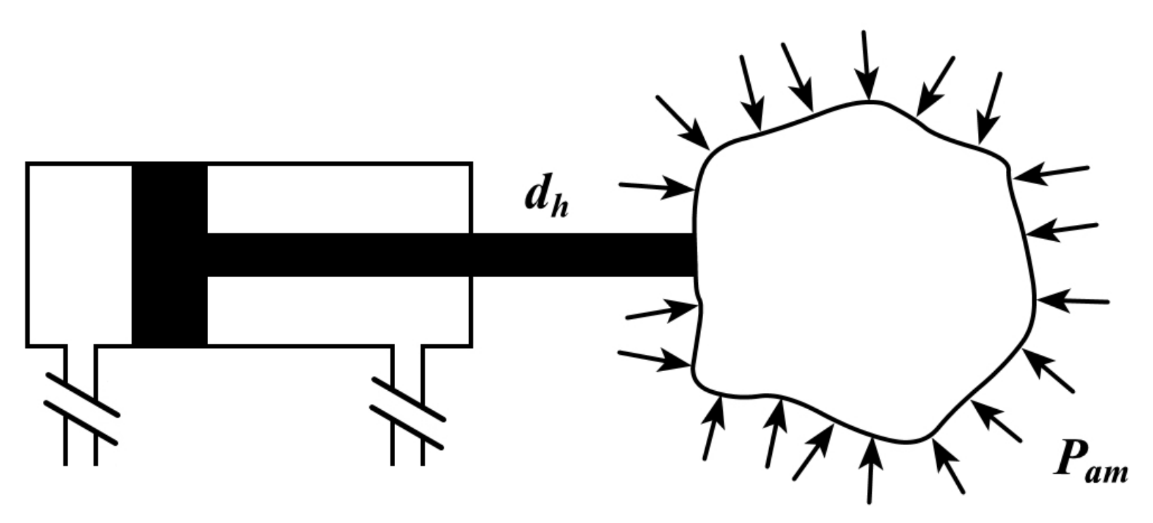
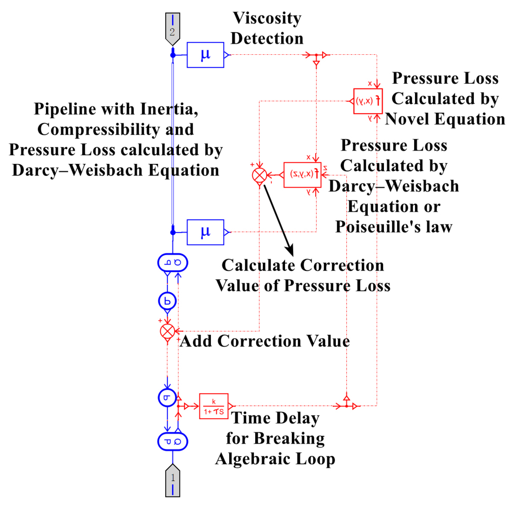
2.5. Slender Pipeline

The pressure compensator, hydraulic pump, relief valve and servo valve are generally closely arranged, and the connecting pipeline between them is much shorter than the slender pipeline between the servo valve and the hydraulic cylinder. Therefore, the pressure loss and dynamics in these pipelines are ignored, and only the ones in slender pipelines connecting the servo valve and the hydraulic cylinder are considered.

The inertia and compressibility of the hydraulic oil in the slender pipeline are calculated by the following two equations, respectively:

$$\dot{Q}=\frac{\pi D^2}{4\rho }\frac{\partial P}{\partial x},$$

(13)

$$\dot{P}=\frac{4{\beta }_e}{\pi D^2}\frac{\partial Q}{\partial x},$$

(14)

where P, Q, and $\rho$ are the pressure, flow rate, and density of the hydraulic oil, respectively, $\partial P/\phantom{\partial P\partial x}\partial x$ and $\partial Q/\phantom{\partial Q\partial x}\partial x$ are the partial derivatives of P and Q along the length of the pipeline, respectively, D is the inner diameter of the pipeline, ${\beta }_e$ is the effective bulk modulus, which is computed as:

$${\beta }_e={\left(\frac{1}{\beta }+\frac{1}{{\beta }_{\mathrm{wall}}}\right)}^{-1},$$

(15)

where $\beta$ is the bulk modulus of hydraulic oil and ${\beta }_{\mathrm{wall}}$ is the wall bulk modulus.

Darcy–Weisbach equation [31], which is expressed as follows for the circular pipeline, is a classic method used to calculate pipeline pressure loss.

$$\Delta P=\lambda \frac{L}{D}\frac{\rho v^2}{2},$$

(16)

where L is the pipeline length, v is the flow velocity, $\rho$ is the density of hydraulic oil, and $\lambda$ is the friction coefficient.

For pipelines with smooth inner surfaces and laminar flow conditions, the friction coefficient is:

$$\lambda =\frac{64}{\mathrm{Re}}.$$

(17)

The Reynolds number $\mathrm{Re}$ is defined as:

$$\mathrm{Re}=\frac{vD}{\nu },$$

(18)

where $\nu$ is the kinematic viscosity of hydraulic oil and its relationship with dynamic viscosity is as follows:

$$\nu =\frac{\eta }{\rho }.$$

(19)

The relationship between flow velocity v and flow rate Q is as follows:

$$Q=\frac{\pi v{D}^2}{4}.$$

(20)

With Equations (17)–(20), Equation (16) can be rewritten as follows:

$$\Delta P=\frac{128\eta LQ}{\pi D^4}.$$

(21)

Equation (21) is exactly the same as Poiseuille’s law.

Equations (13), (14), (16) and (21) are the basic equations of pipeline dynamics and pipeline pressure loss under land conditions. Obviously, the viscosity of the hydraulic oil is treated as a constant.

In deep-sea conditions, the pressure compensator introduces the seawater ambient pressure into the deep-sea VCHCS, which greatly increases the viscosity of the hydraulic oil, and so does the pipeline pressure loss. The large pressure change in the pipeline makes the viscosity of the hydraulic oil increase further when flowing through the pipeline on the basis of the influence caused by the ambient pressure. Therefore, the viscosity change during the pipeline flow should be taken into consideration.

The novel pipeline pressure loss equation proposed in our previous work has taken the above issue into account and it is expressed as follows [28].

$$\Delta P=-\frac{1}{\alpha }ln(1-\frac{128\alpha {\eta }_{0}LQ{e}^{\alpha P_o}}{\pi D^4}),$$

(22)

where $P_o$ is the pipeline outlet pressure and the other symbols have the same meaning as before.

The viscosity-pressure characteristic of hydraulic oil utilized in the novel pipeline pressure loss equation is defined by Equation (1). The novel pipeline pressure loss equation is derived based on the laminar state and has been proved to be equivalent to the classic Poiseuille’s law when the change in viscosity or the pressure loss is small [28].

The viscosity of hydraulic oil increases significantly under deep-sea conditions, then the Reynolds number will decrease according to Equation (18), and the flow state tends to be laminar. Besides, the laminar flow state is usually the state that the hydraulic oil in the pipeline is expected to be in during design because the laminar flow has less energy loss than turbulent flow. Therefore, in this study, Equation (22) will be used to correct the pressure loss calculated by Equation (21) to establish a more accurate model of the deep-sea VCHCS.

Since the viscosity change of the hydraulic oil has no effect on its inertia and compressibility, Equations (13) and (14) are still used for calculating inertia and compressibility, respectively. The pressure losses of pipe elbows and pipe joints are omitted since they are much smaller than the pressure losses in slender pipelines.

2.6. Hydraulic Cylinder

The flow continuity equations of the inlet and outlet ports of the hydraulic cylinder are:

$$Q_1=\frac{V_{01}+A_1{x}_h}{{\beta }_e}{\dot{P}}_1+A_1{\dot{x}}_h+c_l\left(P_1-P_2\right),$$

(23)

$$Q_2=-\frac{V_{02}+A_2{x}_h}{{\beta }_e}{\dot{P}}_2+A_2{\dot{x}}_h+c_l\left(P_1-P_2\right),$$

(24)

where $Q_1$ and $Q_2$ are the flow rates at the two ports of the hydraulic cylinder, $P_1$ and $P_2$ are the pressures at the two ports, $V_{01}$ and $V_{02}$ are the initial volumes of the two chambers of the hydraulic cylinder, $x_h$ is the displacement of the piston in the hydraulic cylinder, $c_l$ is the internal leakage coefficient, and $A_1$ and $A_2$ are the effective areas of the two chambers, which are defined as follows.

$$\left\{\begin{array}{c}{A}_1=\frac{\pi D_h^2}{4},\hfill \\ A_2=\frac{\pi D_h^2}{4}-\frac{\pi d_h^2}{4}.\hfill \end{array}\right.$$

(25)

where $D_h$ and $d_h$ are the piston diameter and rod diameter of the hydraulic cylinder, respectively.

The dynamic equation of the piston is:

$$m_h{\ddot{x}}_h+B_h{\dot{x}}_h-\sum F_{//i}=P_1{A}_1-P_2{A}_2,$$

(26)

where $m_h$ is the mass of the piston, $B_h$ is the viscous friction coefficient, and $F_{//i}$ is the axial component of the force applied to the hydraulic cylinder.

In addition to gravity, buoyancy, and forces from other parts, the hydraulic cylinder is also subjected to the hydrodynamic force and the additional force caused by the ambient pressure in the deep-sea environment. The hydrodynamic force will be analyzed in the next subsection.

For land-based VCHCSs, or deep-sea VCHCSs where the pressure compensator is not taken into consideration, there is no need to count the additional force caused by the ambient pressure. As shown in Figure 2, regardless of the shape of the object connected to the hydraulic cylinder, its outer surface is subjected to the ambient pressure of the seawater. Then, the additional load force caused by the ambient pressure, $F_{am}$, can be deduced as follows:

$$F_{am}=\int P_{am}ds=\frac{\pi d_h^2{P}_{am}}{4},$$

(27)

where $P_{am}$ is the ambient pressure and $d_h$ is the rod diameter of the hydraulic cylinder.

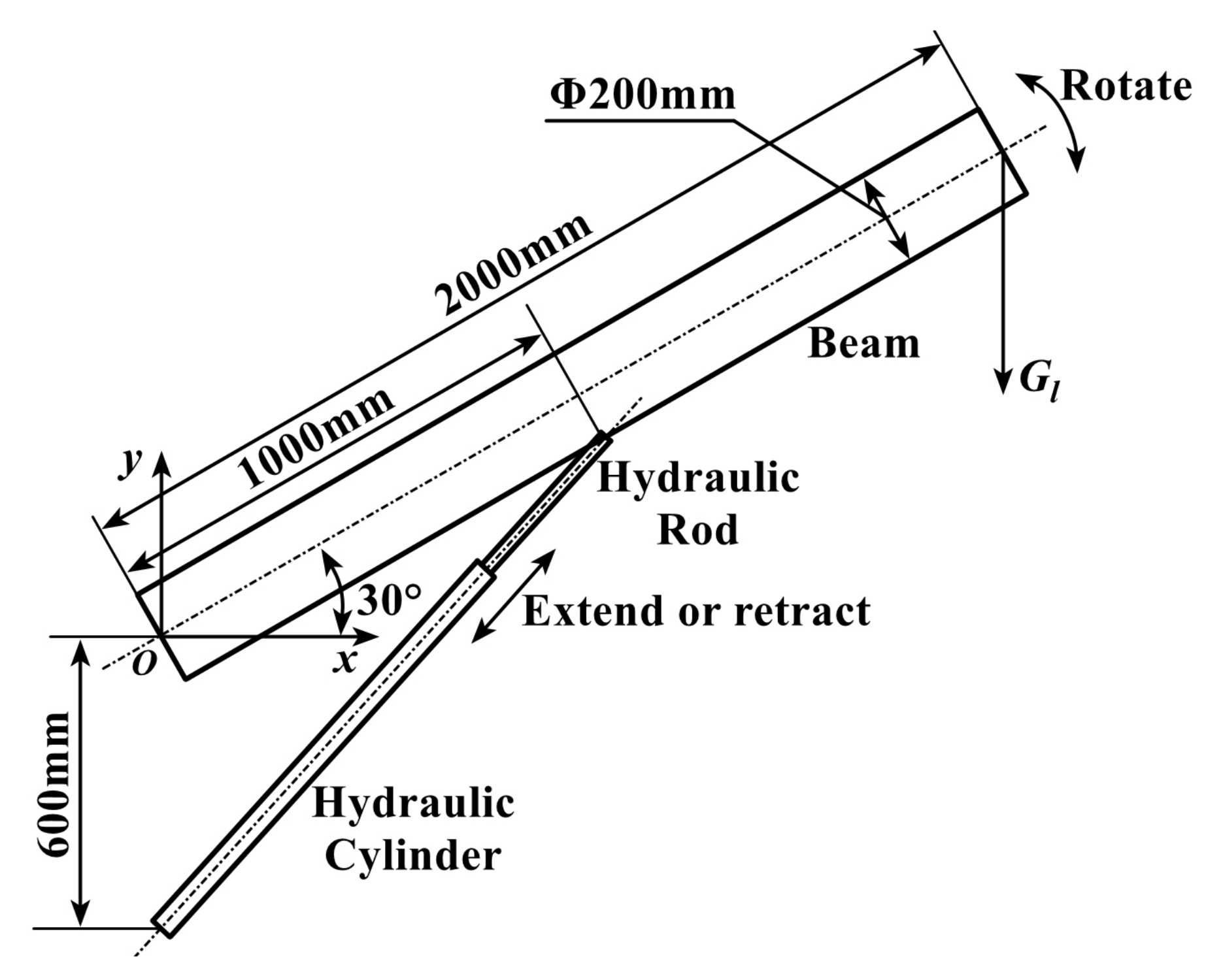
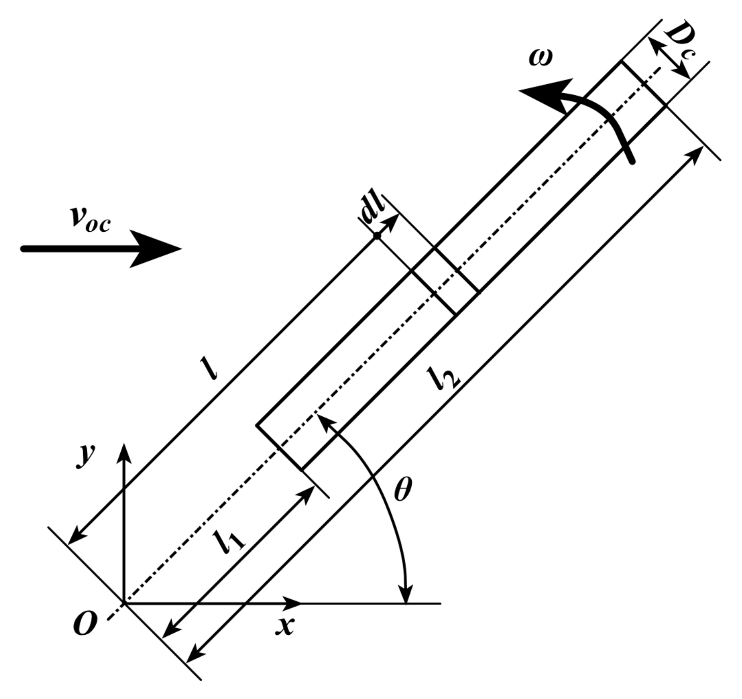
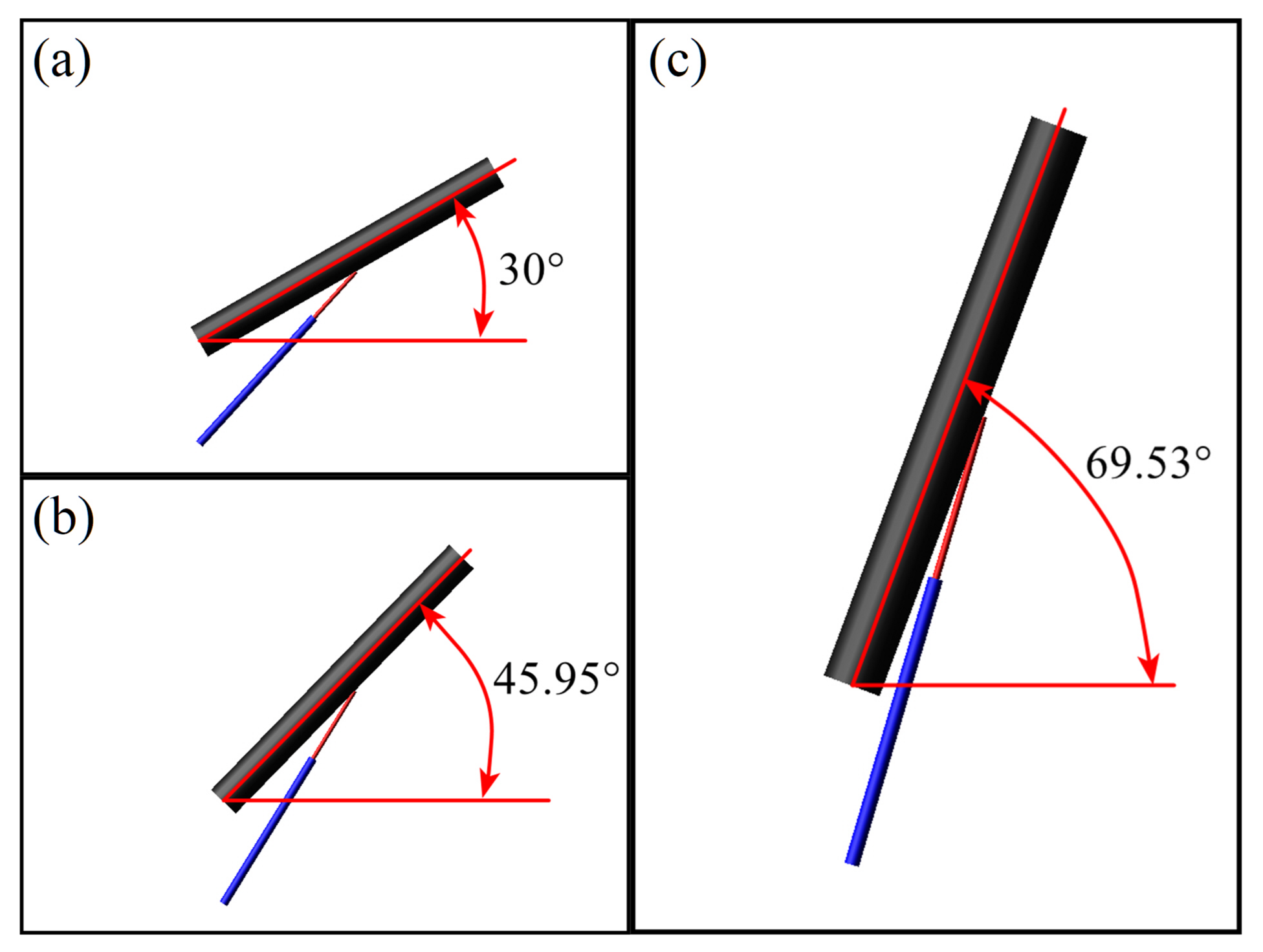
2.7. Mechanical System and Hydrodynamics

As shown in Figure 3, the hydraulic cylinder drives the cylindrical beam to rotate by extending or retracting. The end of the beam is subjected to the gravity of the load mass, $G_l$. Obviously, the beam is also affected by hydrodynamic effect when it rotates in the seawater. Both the beam and the hydraulic cylinder are cylindrical in shape, so a rotating cylinder shown in Figure 4 is taken as the research object to analyze the hydrodynamic load. As shown in Figure 4, the cylinder rotates in the ocean current with a velocity of $v_{oc}$, so the hydrodynamic load on the cylinder consists of two components: the one caused by its own rotation and the one caused by the ocean current.

According to Morrison’s equation [32], the hydrodynamic force applied to the micro-body in the cylinder is:

$$\begin{array}{c}d{F}_{hd}=\frac{1}{2}{\rho }_s·C_D·dA·v_n\left|v_n\right|+{\rho }_s·C_M·dV·\frac{d{v}_n}{dt}\hfill \\ =\frac{1}{2}{\rho }_s·C_D·D_c·dl·v_n\left|v_n\right|+{\rho }_s·C_M·\frac{\pi D_c^2}{4}·dl·\frac{d{v}_n}{dt},\hfill \end{array}$$

(28)

where $d{F}_{hd}$ is the hydrodynamic force applied to the micro-body, ${\rho }_s$ is the density of the seawater, $C_D$ and $C_M$ are the drag coefficient and inertia coefficient respectively, $dl$, $dA$ and $dV$ are the length, projected area and volume of the micro-body respectively, $D_c$ is the cylinder diameter, and $v_n$ is the normal velocity of the relative motion between the micro-body and the seawater.

Based on Equation (28), the hydrodynamic torque caused by its own rotation, $M_{hd-r}$, and the hydrodynamic torque caused by the ocean current, $M_{hd-oc}$, are derived and then expressed as follows. For the detailed derivation process, please refer to Appendix A.

$$M_{hd-r}=\frac{1}{8}{\rho }_s{C}_D{D}_c\omega \left|\omega \right|\left(l_2^4-l_1^4\right)+\frac{1}{12}{\rho }_s{C}_M\pi D_c^2·\frac{d\omega }{dt}·\left(l_2^3-l_1^3\right),$$

(29)

$$M_{hd-oc}=\frac{1}{2}{\rho }_s{C}_D{D}_c{v}_{oc}\left|v_{oc}\right|{sin}^2\theta \left(l_2^2-l_1^2\right)+\frac{1}{8}{\rho }_s{C}_M\pi D_c^{2}sin\theta ·\frac{d{v}_{oc}}{dt}·\left(l_2^2-l_1^2\right),$$

(30)

where $l_1$ and $l_2$ are the distances from the two ends of the cylinder to the origin, respectively, $\omega$ is the angular velocity of the cylinder, $\theta$ is the inclination angle of the cylinder, and $v_{oc}$ is the velocity of the ocean current.

The small size of the cylinder has minimal impact on ocean currents, so the two deduced hydrodynamic torques can be superimposed. Therefore, the total hydrodynamic torque applied to the cylinder, $M_{hd}$, can be expressed as follows.

$$M_{hd}=M_{hd-r}+M_{hd-oc}.$$

(31)

With Equations (29)–(31), the hydrodynamic load can be applied to the cylindrical beam and hydraulic cylinder.

3. Model and Settings

Based on the basic equations and assumptions in the previous section, a co-simulation model of the deep-sea VCHCS is built based on the AME Sim and ADAMS platforms. The AME Sim model of the hydraulic system is shown in Figure 5. The slender pipeline in Figure 5 is encapsulated, and the detailed model of the slender pipeline is shown in Figure 6. The ADAMS model of the mechanical system is shown in Figure 7. The hydraulic model transmits the force signal to the mechanical model, while the mechanical model transmits displacement and velocity signals to the hydraulic model.

The AME Sim model shown in Figure 5 is consistent with the schematic diagram shown in Figure 1. For the slender pipeline model, AME Sim’s own pipeline model is used to calculate the inertia and compressibility of the hydraulic oil. The pressure loss is also calculated based on the Darcy–Weisbach equation in the AME Sim’s own pipeline model. With the lower one of the viscosities at the pipeline ports and the inlet flow rate, the pressure loss based on the Darcy–Weisbach equation or Poiseuille’s law is calculated with a user-defined function, in which the viscosity change is not considered. With the viscosity at the pipeline outlet and the inlet flow rate, the pressure loss considering the viscosity change is also calculated with a user-defined function according to the novel equation expressed by Equation (22). Then the correction value of pressure loss can be obtained by subtracting the aforementioned two pressure losses, and it is used to correct the pressure output of AME Sim’s own pipeline model. A first-order lag is utilized to introduce the time delay for breaking the algebraic loop between the slender and the servo valve. When the time constant of the first-order lag is much smaller than the calculation step size in the model, the change in dynamic characteristics caused by the first-order lag can be ignored. In addition, the model also includes a hydraulic cylinder displacement sensor and a PID controller.

The ADAMS model shown in Figure 7 is consistent with the mechanical system shown in Figure 3. Hydrodynamic loads are applied to each moving part according to Equations (29)–(31).

The parameter settings in the co-simulation model are listed in Appendix B. The viscosity–pressure index $\alpha$ of the hydraulic oil is within $1.5\times {10}^{-8}$Pa${}^{-1}$ to $3.5\times {10}^{-8}$Pa${}^{-1}$ [33,34]. It is set as $2.2\times {10}^{-8}$Pa${}^{-1}$ in the model, which is the viscosity-pressure index of the HFD fire-resistant hydraulic oil [34]. Servo valve parameter settings refer to the product catalog of [35]. In the AME Sim platform, with the rated flow at maximum valve opening and the corresponding pressure drop of the servo valve, the equivalent orifice area and the hydraulic diameter can be computed [36]. The equivalent orifice shows the same characteristics that complies with Equation (8) or (9). The ambient pressure increases by 10 MPa for each increase of 1km in depth.

The simulation step and convergence tolerance are 0.001 s and $1\times {10}^{-5}$, respectively. The simulation type is dynamic, and the solver type in AME Sim is regular.

Before starting the simulation of the deep-sea VCHCS on various working conditions, with a flow source added to the inlet and outlet pressure set as ambient pressure, the slender pipeline considering pressure-dependent viscosity is simulated and compared with AME Sim’s own pipeline.

4. Results and Discussions

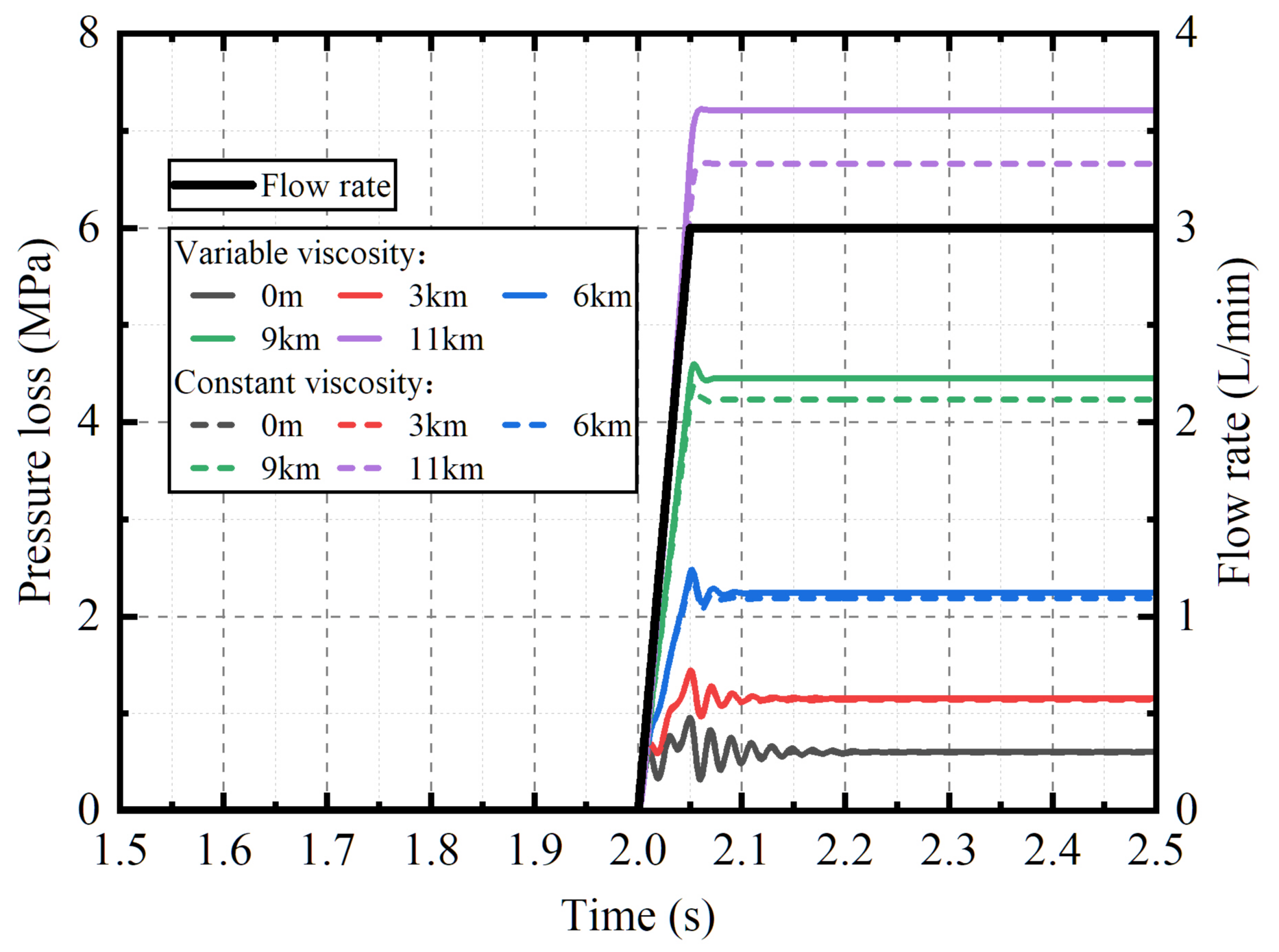
4.1. Slender Pipeline

With a flow rate of 3L/min, according to Figure 8, when the working depth is less than or equal to 3 km, the dynamic response and pressure loss of the slender pipeline with variable viscosity are basically the same as those with constant viscosity. However, when the working depth is 6 km or above, the dynamic response and pressure loss are no longer the same, and the deeper the depth is, the greater the difference is. When the depth is 11 km, the stable pressure losses are 7.2067 MPa and 6.6593 MPa respectively, and the difference is 8.22%. Then we can conclude that in the deep-sea VCHCS, the viscosity change of the hydraulic oil in the slender pipeline needs to be considered to more accurately simulate the performance of the system.

Table 1. Pressure losses.

No.	Viscosity-Pressure Index	Initial Kinematic Viscosity	Pipeline Length	Pipeline Inner Diameter	Depth	Flow Rate	Simulated Pressure Loss	Theoretical Pressure Loss	Error
	(Pa${}^{-1}$)	(cSt)	(m)	(mm)	(km)	(L/min)	(MPa)	(MPa)	(%)
1	$2.2\times {10}^{-8}$	22	4	4	6	3	2.2421	2.2847	−1.86
2	$1.5\times {10}^{-8}$	22	4	4	6	3	1.4333	1.4804	−3.18
3	$3\times {10}^{-8}$	22	4	4	6	3	2.5693	2.3281	4.53
4	$2.2\times {10}^{-8}$	10	4	4	6	3	0.9920	1.0243	−3.15
5	$2.2\times {10}^{-8}$	32	4	4	6	3	3.3365	3.3624	−0.77
6	$2.2\times {10}^{-8}$	22	3	4	6	3	1.6608	1.7027	−2.46
7	$2.2\times {10}^{-8}$	22	5	4	6	3	2.8378	2.8743	−1.27
8	$2.2\times {10}^{-8}$	22	4	3	6	3	7.9246	7.6517	3.57
9	$2.2\times {10}^{-8}$	22	4	5	6	3	0.8920	0.9920	−3.25
10	$2.2\times {10}^{-8}$	22	4	4	0	3	0.6043	0.6005	0.63
11	$2.2\times {10}^{-8}$	22	4	4	11	3	7.2067	7.2413	−0.48
12	$2.2\times {10}^{-8}$	22	4	4	6	2	1.4702	1.5103	−2.66
13	$2.2\times {10}^{-8}$	22	4	4	6	4	3.0397	3.0725	−1.07

lists the simulation values of the pressure loss with variable viscosity under different parameters, and the theoretical value calculated according to Equation (22) is also listed for comparison. For all the cases in Table 1, the errors between the simulated and theoretical pressure losses are all within ±5%. Then, it can be known that the slender pipeline established in this paper, in which the pressure-dependent viscosity change of hydraulic oil is considered, is reasonable.

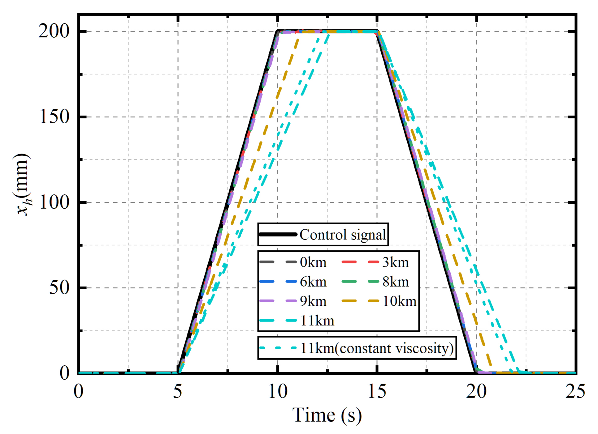
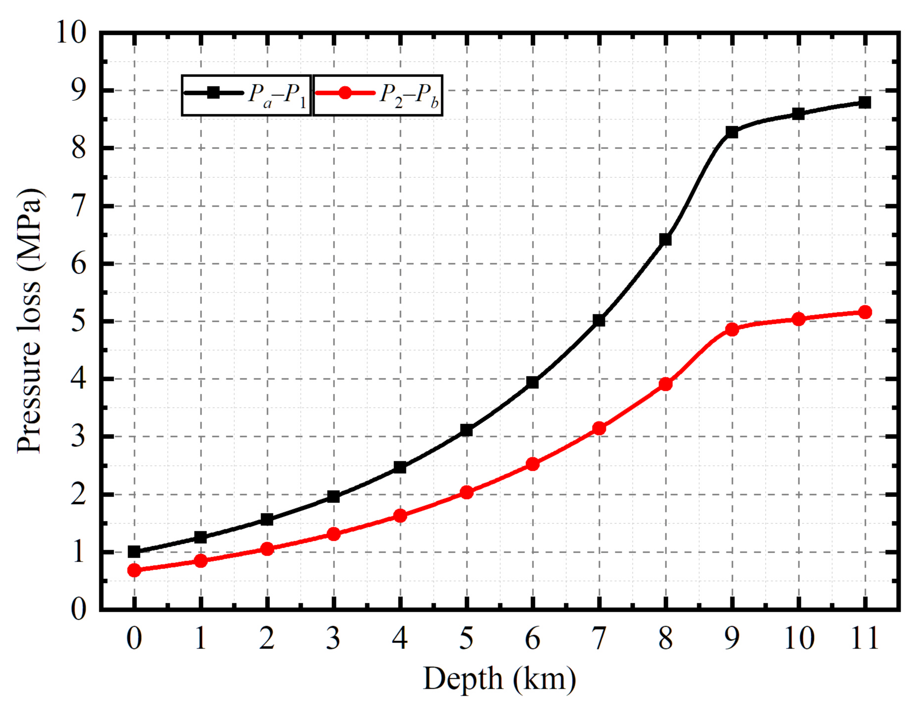
4.2. Working Performance of Deep-Sea VCHCS at Different Depths

The control signal is set to linearly extend to 200 mm within 5 s and retract to 0 mm within 5 s, as shown in Figure 9. In other words, the target extension or retraction velocity of the hydraulic cylinder is 40 mm/s. According to Figure 9, when the depth in the sea is less than or equal to 9 km, the displacement output of the hydraulic cylinder, $x_h$, is consistent with the control signal, indicating that there is no delay. However, when the depth is greater than or equal to 10 km, $x_h$ is delayed compared to the control signal, and the deeper the depth is, the more serious the delay is. When the depth is 11 km, which is about the depth of Mariana’s bottom, the extension time and retraction time of the hydraulic cylinder are 7.625 s and 7.156 s, respectively. Compared with the action time of 5 s set by the control signal, the extension and retraction actions are delayed by 52.50% and 43.12%, respectively. The spatial states of the mechanical system at different $x_h$ are shown in Figure 10.

For comparison, $x_h$ with the AME Sim own pipeline, in which the viscosity of the hydraulic oil is treated as a constant value, is also plotted in Figure 9. $x_h$ with the constant-viscosity pipeline model is still delayed, but it responds faster than that of the variable-viscosity pipeline model. The extension time and the retraction time with the constant-viscosity pipeline model are 7.178 s and 6.779 s, respectively. Compared with the variable-viscosity pipeline model, the deviation values are 0.447 s and 0.377 s, respectively. Then it can be known that the viscosity change of the hydraulic oil in the slender pipeline has a significant impact on the displacement output of the deep-sea VCHCS and should be considered to make the model more accurate.

The root cause of the delay in the displacement output of the deep-sea VCHCS is discussed as follows. When the hydraulic cylinder is extending, the pressure losses in the two slender pipelines are shown in Figure 11. It can be known from Figure 11 and Equation (1) that as the depth and the ambient pressure of the seawater increase, the viscosity of the hydraulic oil increases sharply, and as a result, the pipeline pressure loss increases significantly. Among them, when the depth is greater than 9 km, the increase in pressure loss slows down. This is because the hydraulic cylinder has been delayed in movement in these working conditions, which are as shown in Figure 9, and the corresponding flow rates are less than the flow rates at other depths.

The pressure at port p of the servo valve is equal to the set cracking pressure of the relief valve. Since the depth increases and subsequently the pressure loss in the slender pipeline increases, the pressure difference between the ports p and a of the servo valve decreases when the hydraulic cylinder is extending, which is as shown by the black curve in Figure 12. To ensure that the flow rate is still consistent with the flow rate that matches the control signal, according to Equation (8), the displacement of the servo valve spool needs to be increased, which is as shown by the red curve in Figure 12, and so as to increase the flow area of the servo valve. However, when the depth is 10km or more, the servo spool has reached its maximum stroke and cannot continue to increase the flow area, which means that the flow rate cannot be increased to the one that matches the control signal. Eventually, the extension speed of the hydraulic cylinder decreases, as shown by the blue curve in Figure 12, and a delay in the output displacement of the hydraulic cylinder when extending, as shown in Figure 9, occurs. When the hydraulic cylinder is retracting, the cause of the delay is similar to the above analysis.

According to the above analysis, reducing the pressure loss in the slender pipeline, increasing the pressure difference and the maximum flow capacity of the servo valve can all improve or even eliminate the delay phenomenon of the deep-sea VCHCS. These will be analyzed and discussed in the next subsection based on the established co-simulation model.

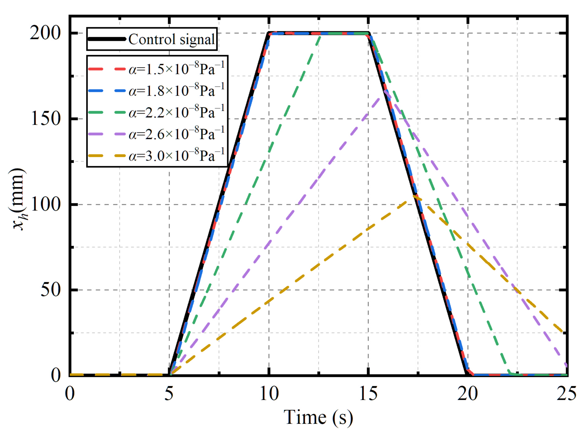
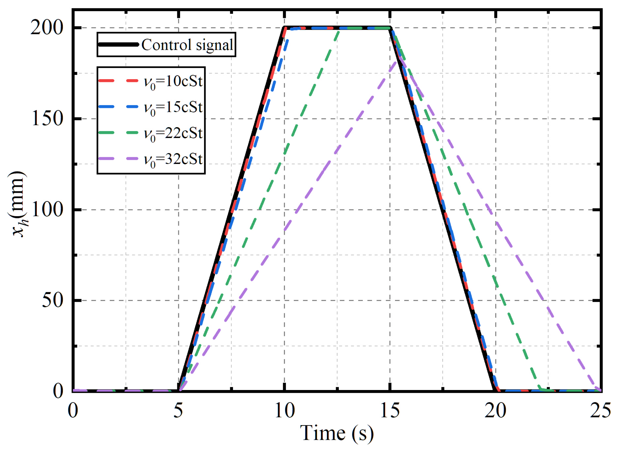
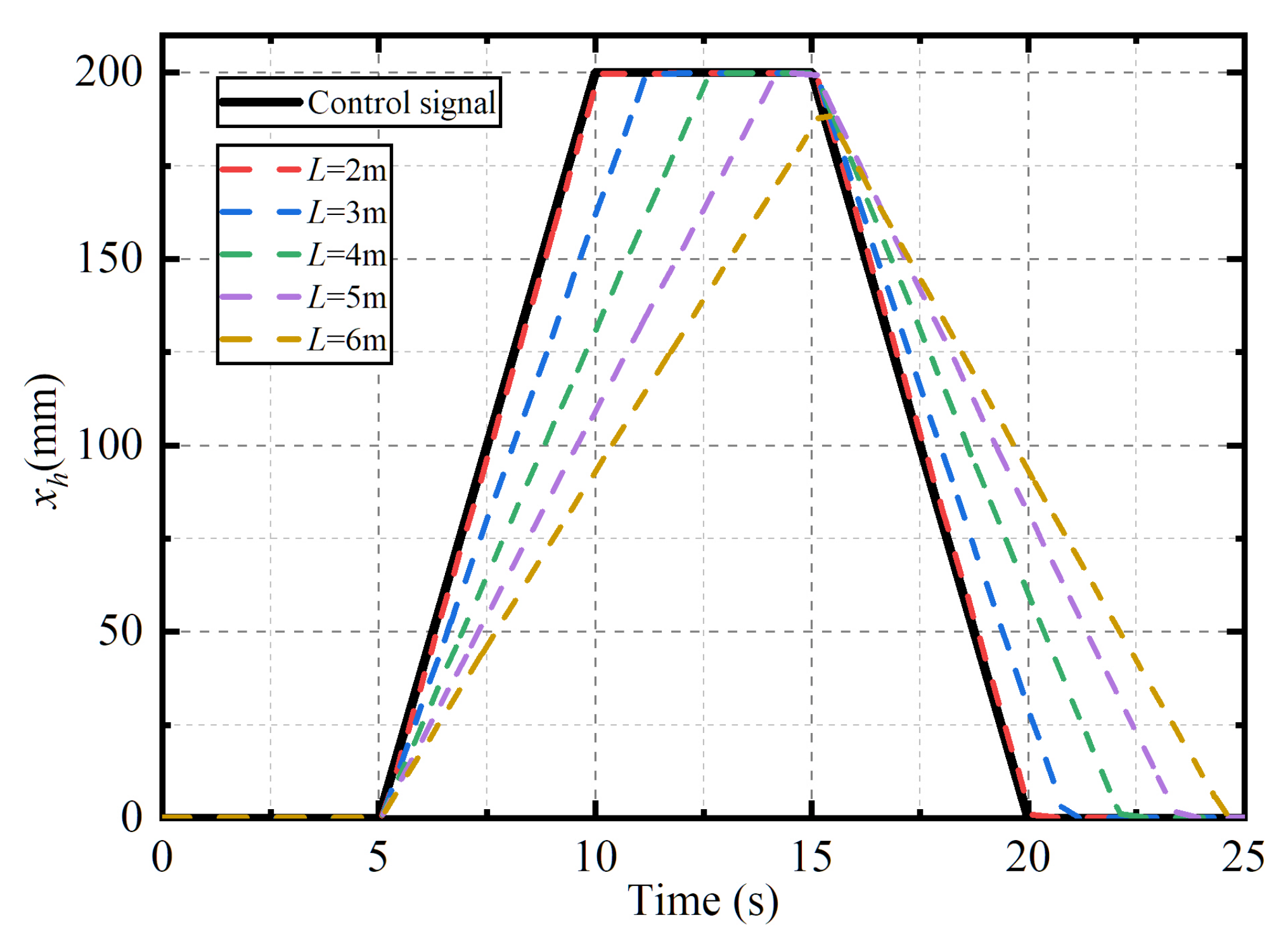
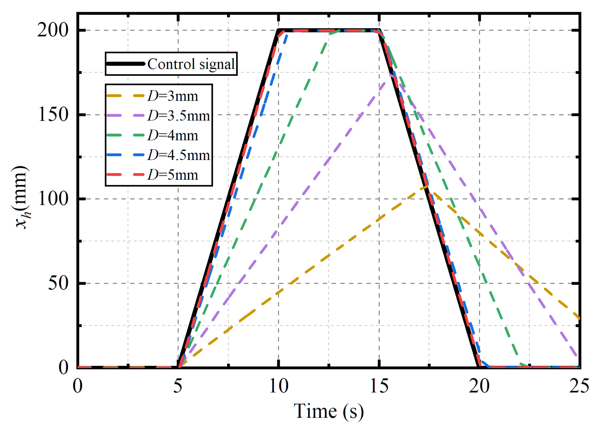
4.3. Parameter Study

4.3.1. System Parameter of Deep-Sea VCHCS

a. Viscosity-pressure index of hydraulic oil.

The direct cause of the delay in the deep-sea VCHCS is the sharp increase in the pipeline pressure loss. The essence of pipeline pressure loss is the need to overcome the friction caused by the viscosity of the hydraulic oil when flowing through the pipeline. According to Equation (1), it is obvious that the viscosity of hydraulic oil increases exponentially with the ambient pressure introduced by the pressure compensator. The factor that measures the viscosity of hydraulic oil affected by pressure is the viscosity-pressure index $\alpha$. According to Figure 13, when the depth is 11km, the greater the viscosity-pressure index $\alpha$ is, the more serious the delay in $x_h$ is. Among them, when $\alpha$ is less than or equal to $1.8\times {10}^{-8}$ Pa${}^{-1}$, there is no delay in $x_h$. In summary, the use of hydraulic oil with a small viscosity-pressure index $\alpha$ can result in smaller pipeline pressure losses in the deep-sea VCHCS and better response performance of the displacement output.

b. Initial viscosity of hydraulic oil.

In addition to the pressure-viscosity index $\alpha$, according to Equation (1), the initial viscosity of the hydraulic oil when it is not subjected to ambient pressure also affects the viscosity of the hydraulic oil under the influence of the ambient pressure introduced by the pressure compensator. Then the initial viscosity of the hydraulic oil also affects the performance of the deep-sea VCHCS. According to Figure 14, when the depth is 11 km, the greater the initial kinematic viscosity of hydraulic oil, ${\nu }_0$, is, the more serious the delay in $x_h$ is. Among them, when ${\nu }_0$ is 10 cSt, there is no delay in $x_h$. Obviously, the use of hydraulic oil with a lower initial viscosity also helps to reduce or even eliminate the displacement output delay of the deep-sea VCHCS.

c. Pipeline length.

According to Equation (22), the geometric dimensions of the slender pipeline obviously also affect the pipeline pressure loss, which in turn also affects the displacement output of the deep-sea VCHCS. One of the influencing factors is the pipeline length L. The larger the pipeline length L is, the larger the pressure loss in the slender pipeline is, and as shown in Figure 15, the more serious the delay in $x_h$ is. Among them, when L is 2 m, there is no delay in $x_h$. Although the smaller the pipeline length L is, the better the response performance is, the determination of L needs to give priority to meeting the basic length requirements of the spatial layout of the entire system.

d. Pipeline inner diameter.

Another geometric dimension of the slender pipeline that affects the pressure loss and then the displacement output of the deep-sea VCHCS, $x_h$, is the pipeline inner diameter D, according to Equation (22). Given that the index of D in Equation (22) is 4, the pressure loss and $x_h$ are very sensitive to changes in D. It can be seen from Figure 16 that a change in D as small as 1 mm or only 0.5 mm can greatly affect $x_h$ at a depth of 11 km, and there is no delay in $x_h$ when D is 5 mm. Based on the above analysis and discussion, it can be seen that the use of pipelines with a larger inner diameter can greatly improve the response performance of the deep-sea VCHCS. It should be noted that pipelines with an excessively large diameter, which are filled with hydraulic oil, are also an additional burden on the deep-sea hydraulic manipulator. Therefore, when the pipeline pressure loss has been decreased within an acceptable range, the pipeline inner diameter D does not need to be further increased.

e. Rated flow of servo valve.

According to the analysis and discussion in Section 4.2, when the displacement output delay of the deep-sea VCHCS occurs, the servo valve has reached its maximum flow area. Therefore, it is obvious that increasing the maximum flow capacity of the servo valve can also help reduce the delay. Figure 17 plots the displacement output of the deep-sea VCHCS, $x_h$, when working at athe depth of 11 km with different servo valves, whose rated flows, $Q_{Rsv}$, refer to the product catalog of [35]. Figure 17 clearly indicates that the smaller $Q_{Rsv}$ is, in other words, the smaller the flow capacity of the servo valve is, the more serious the delay is. However, when $Q_{Rsv}$ is greater than 10 L/min, according to Figure 17, the effect of increasing $Q_{Rsv}$ on reducing the delay in $x_h$ is no longer obvious. The root cause of this phenomenon is that, despite the increase in the flow capacity of the servo valve, the pressure loss of the slender pipeline has not been reduced, meaning that the pressure difference between the ports of the servo valve is still very small.

f. Cracking pressure of relief valve.

In addition to reducing pipeline pressure losses, another way to increase the pressure difference between the servo valve ports is to increase the inlet pressure of the servo valve, that is, to increase the cracking pressure of the relief valve, $P_{rv}$. It can be known from Figure 18 that increasing $P_{rv}$ can reduce the displacement output delay of the deep-sea VCHCS at a depth of 11 km. However, it should be noted that a greater $P_{rv}$ can result in more energy loss due to the overflow through the relief valve.

4.3.2. Input Parameter of Deep-Sea VCHCS

In addition to the parameters of the deep-sea VCHCS itself, its inputs also affect its working performance. Inputs include working depth, control signal, and loads. The influence of the working depth has been discussed in Section 4.2, and the remaining two inputs will be analyzed and discussed below.

a. Input signal.

Controlled by four different input signals, namely linearly extending to 100 mm, 150 mm, 200 mm, or 220 mm within 5 s, and retracting to 0 mm within 5 s, the displacement outputs of the deep-sea VCHCS, $x_h$, at the depth of 11 km are all plotted in Figure 19. It can be seen from Figure 19 that when the maximum control signal is 220 mm, 200 mm, and 150 mm, the corresponding $x_h$ are all delayed. These displacement outputs coincide with each other when extending and are parallel to each other when retracting. The phenomenon of coincidence and parallelism when delayed is because the servo valve is all working in the state with maximum flow area under these conditions, as described in Section 4.2. When the maximum control signal is 100 mm, there is no delay in $x_h$. This is because the required flow rate corresponding to this control signal is within the flow capacity range of the servo valve at 11 km in the deep sea. From the above analysis, it can be known that when the delay in $x_h$ occurs, the most direct solution is to make the target or the expected displacement control signal change more slowly with time, that is, to make the target speed lower. Although such a solution increases the operation time and reduces work efficiency, it can ensure the accuracy of the displacement output without any adjustments to the deep-sea VCHCS.

b. Loads.

The external loads on the mechanical system include three components: the gravity of the load mass, the hydrodynamic load, and the ambient load. The pressure compensator introduces the ambient pressure $P_{am}$ into the hydraulic system. According to the effective area on both sides of the hydraulic cylinder expressed by Equation (25), it can be known that the hydraulic cylinder has an output force of $\pi d_h^2{P}_{am}/\phantom{\pi d_h^2{P}_{am}4}4$, which equals the ambient pressure load expressed by Equation (27). Then, it can be known that the ambient pressure load is inherently balanced and does not need to be considered.

b.1. Gravity of load mass.

As for the gravity of load mass, $G_l$, as shown in Figure 20, the greater $G_l$ is, the more serious the delay is when extending, but the less serious the delay is when retracting. The reason for this phenomenon is that, according to the mechanical system shown in Figure 3, $G_l$ has the effect of promoting the retraction of the hydraulic cylinder.

b.2. Hydrodynamic load.

As analyzed in Section 2.7, hydrodynamic effects consist of two components: those caused by the motion of the mechanical system itself and those caused by ocean currents. Due to the slow movement speed of the mechanical system in this study, the hydrodynamic effect caused by the movement of the mechanical system itself is much smaller than that caused by the ocean current, so only the influence of the hydrodynamic effect caused by the ocean current will be discussed below.

According to Figure 21, a positive velocity of ocean current, $v_{oc}$, exacerbates the delay in $x_h$ compared to the case without ocean current when extending at a depth of 11 km. However, when retracting, a positive $v_{oc}$ makes $x_h$ response faster. As for negative $v_{oc}$, the opposite is true, that is, $x_h$ responds faster when extending but slower when retracting. In addition, the larger the magnitude of $v_{oc}$ is, the more severe the above impact is. This phenomenon can be explained as follows. From Figure 3 and Figure 4, it can be known that the hydrodynamic force caused by a positive $v_{oc}$ tends to make the hydraulic cylinder retract, while the one caused by a negative $v_{oc}$ tends to make the hydraulic cylinder extend. This makes the deep-sea VCHCS more prone to the delay in $x_h$ when the mechanical system moves against ocean currents.

5. Conclusions

1.

A detailed nonlinear mathematical model of the deep-sea VCHCS is described. In the model, the viscosity change of the hydraulic oil when flowing through the pipeline is considered based on the viscosity-pressure characteristics of the hydraulic oil. So is the viscosity increase caused by the pressure-compensator-introduced ambient pressure. With Morrison’s equation, the hydrodynamic effects are also included in the model.

2.

Based on the nonlinear mathematical model, the corresponding numerical co-simulation model of the deep-sea VCHCS is established. The verification simulation of the slender pipeline model indicates that the viscosity change of the hydraulic oil when flowing through the pipeline has a significant impact when the depth is greater than or equal to 6 km. The errors between the simulated pressure loss of the slender pipeline and the theoretical one are all within ±5% under various conditions.

3.

Based on the numerical co-simulation model, the working performance of the deep-sea VCHCS at different depths in the sea is analyzed. When the depth is greater than or equal to 10 km, the output displacement of the hydraulic cylinder is delayed, and the deeper the depth is, the more serious the delay is. Compared with the control signal, the extension and retraction time of the hydraulic cylinder are delayed by 52.50% and 43.12%, respectively, when the depth is 11 km.

4.

The essential logic of the delay phenomenon is as follows. The pressure compensator introduces the ambient pressure into the deep-sea VCHCS, which makes the viscosity of the hydraulic oil increase greatly with the increase in depth, and so does the pressure loss in the slender pipeline. Therefore, the pressure difference of the servo valve decreases as the depth increases, and the servo valve needs to increase its flow area to maintain a flow rate that matches the control signal. When the servo valve is in the state with the maximum flow area, the flow rate matching the control signal can no longer be provided, and, finally, the displacement output is delayed.

5.

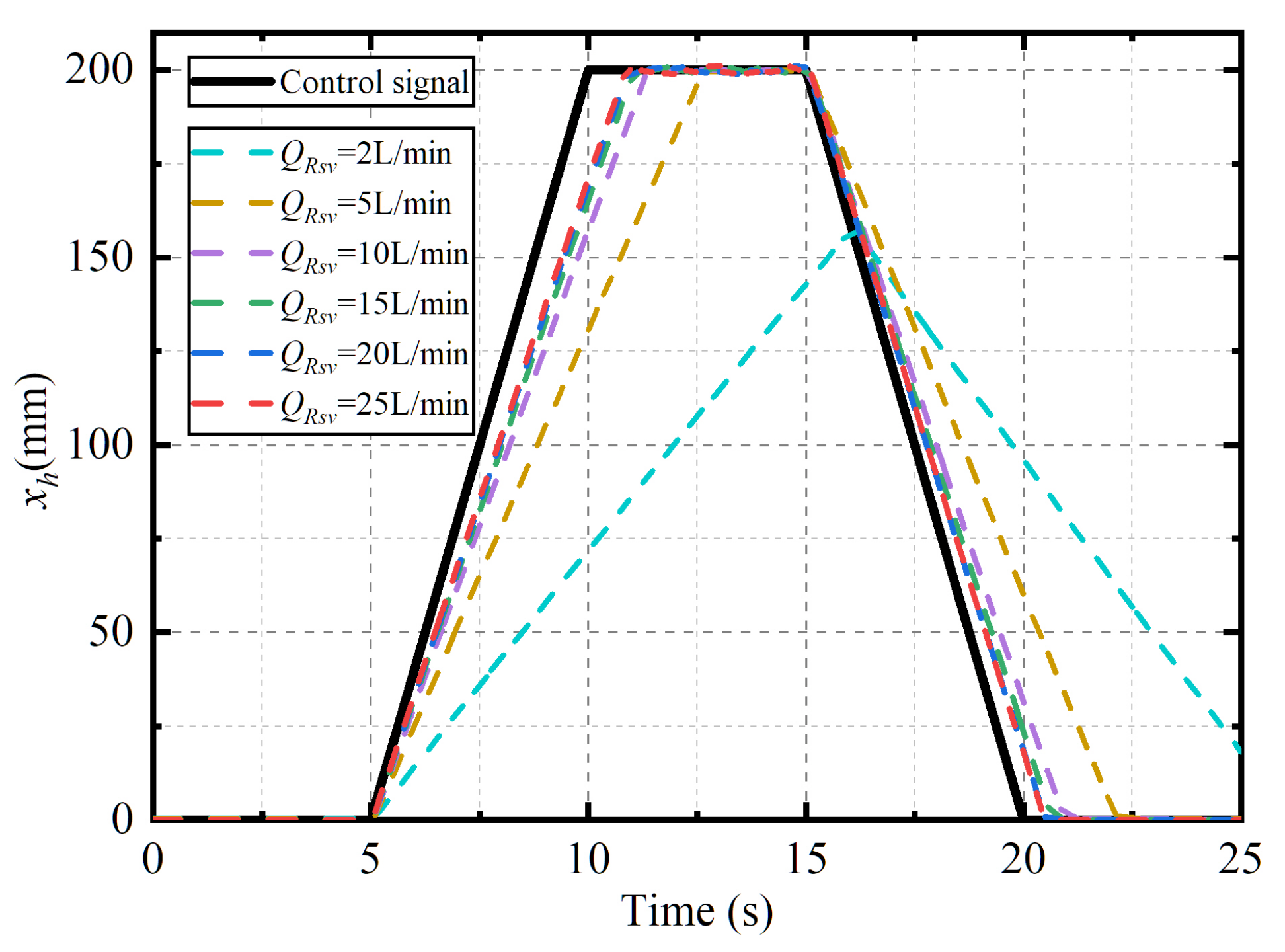
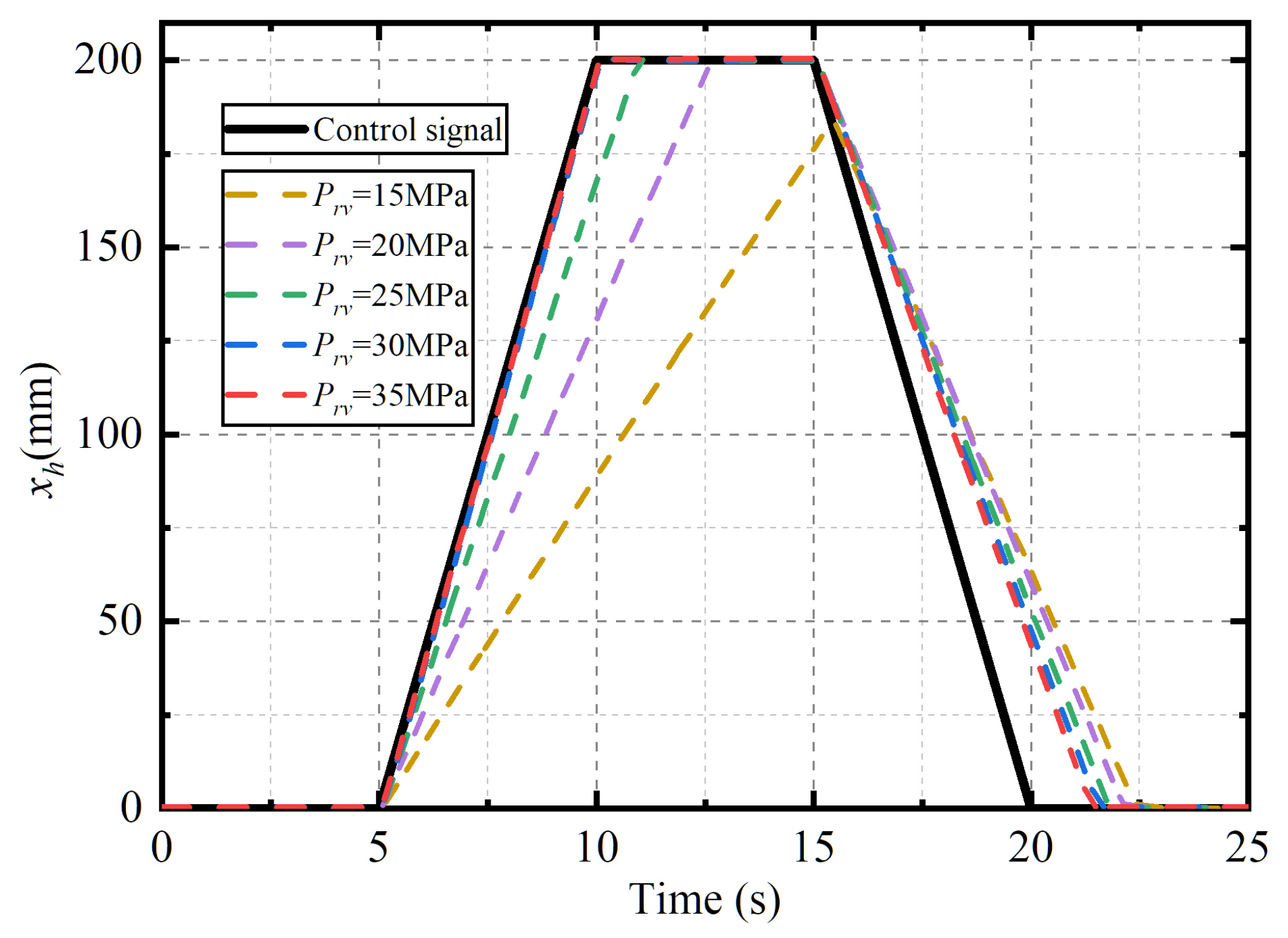
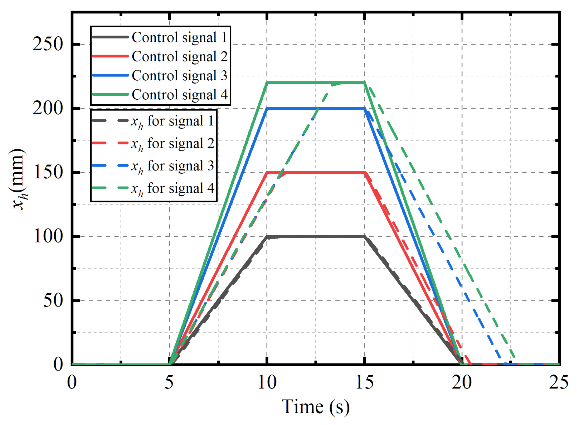
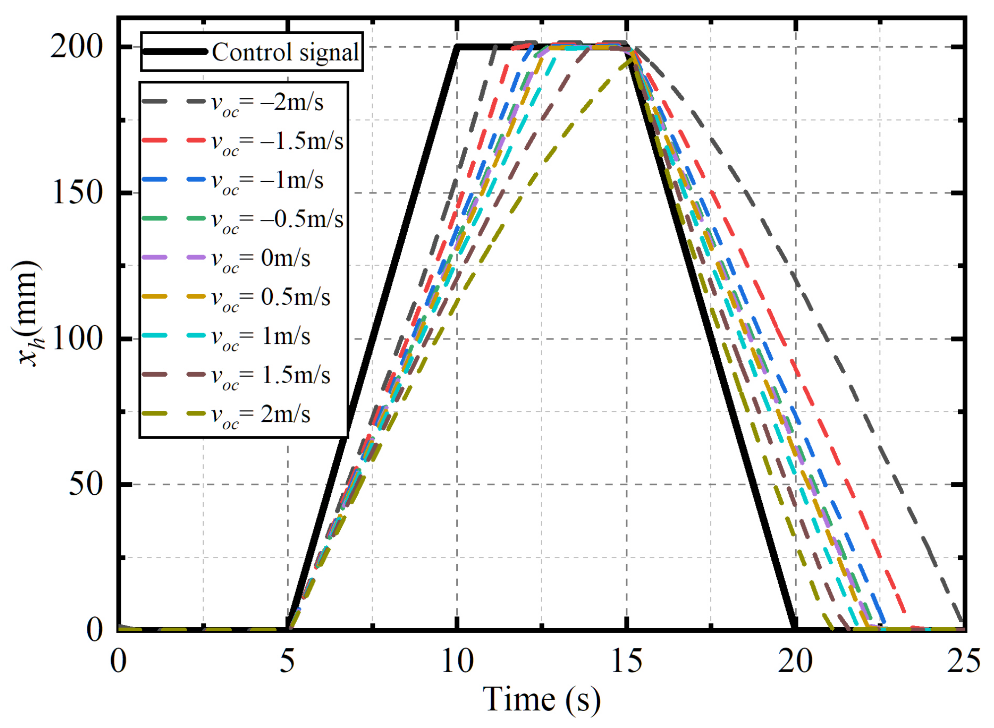
Measures to reduce or even eliminate the displacement output delay when designing a deep-sea VCHCS include: selecting hydraulic oil with a small viscosity-pressure index and initial viscosity, reducing the length of the slender pipeline, increasing the inner diameter of the slender pipeline, selecting a servo valve with a large rated flow, increasing the cracking pressure of the relief valve. Control signals and loads also affect the displacement output delay. Among them, the movement against the ocean current of the mechanical system can make the deep-sea VCHCS more prone to delay due to the additional hydrodynamic load.

References

1. Sivčev, S.; Coleman, J.; Omerdić, E.; Dooly, G.; Toal, D. Underwater manipulators: A review. Ocean. Eng. 2018, 163, 431–450. [Google Scholar] [CrossRef]
2. Sartore, C.; Simetti, E.; Wanderlingh, F.; Casalino, G. Autonomous Deep Sea Mining Exploration: The EU ROBUST Project Control Framework. In Proceedings of the OCEANS 2019-Marseille, Marseille, France, 17–20 June 2019; pp. 1–8. [Google Scholar] [CrossRef]
3. Lynch, B.; Ellery, A. Efficient Control of an AUV-Manipulator System: An Application for the Exploration of Europa. IEEE J. Ocean. Eng. 2014, 39, 552–570. [Google Scholar] [CrossRef]
4. Wang, C.; Zhang, Q.; Zhang, Q.; Zhang, Y.; Huo, L.; Wang, X. Construction and Research of an Underwater Autonomous Dual Manipulator Platform. In Proceedings of the 2018 OCEANS-MTS/IEEE Kobe Techno-Oceans (OTO), Kobe, Japan, 28–31 May 2018; pp. 1–5. [Google Scholar] [CrossRef]
5. Sivčev, S.; Rossi, M.; Coleman, J.; Omerdić, E.; Dooly, G.; Toal, D. Collision Detection for Underwater ROV Manipulator Systems. Sensors 2018, 18, 1117. [Google Scholar] [CrossRef] [PubMed] [Green Version]
6. Fan, Y.; Zhang, Q.; Wang, H.; Bai, Y.; Zhang, Y.; Cui, S. Design and Experiments of a 11000m 7-Function Electric Manipulator System. In Proceedings of the 2018 OCEANS-MTS/IEEE Kobe Techno-Oceans (OTO), Kobe, Japan, 28–31 May 2018; pp. 1–4. [Google Scholar] [CrossRef]
7. Bai, Y.; Zhang, Q.; Tian, Q.; Yan, S.; Tang, Y.; Zhang, A. Performance and experiment of deep-sea master-slave servo electric manipulator. In Proceedings of the OCEANS 2019 MTS/IEEE SEATTLE, Seattle, WA, USA, 27–31 October 2019; pp. 1–5. [Google Scholar] [CrossRef]
8. Zhang, Y.; Zhang, Q.; Zhang, A.; Cui, S.; Du, L.; Huo, L. Experiment research on control performance for the actuators of a deep-sea hydraulic manipulator. In Proceedings of the OCEANS 2016 MTS/IEEE Monterey, Monterey, CA, USA, 19–23 September 2016; pp. 1–6. [Google Scholar] [CrossRef]
9. Chen, Y.; Zhang, Q.; Tian, Q.; Huo, L.; Feng, X. Fuzzy Adaptive Impedance Control for Deep-Sea Hydraulic Manipulator Grasping Under Uncertainties. In Proceedings of the Global Oceans 2020: Singapore–U.S. Gulf Coast, Biloxi, MS, USA, 5–30 October 2020; pp. 1–6. [Google Scholar] [CrossRef]
10. Liu, Y.; Wu, D.; Li, D.; Deng, Y. Applications and Research Progress of Hydraulic Technology in Deep Sea. J. Mech. Eng. 2018, 54, 14–23. [Google Scholar] [CrossRef]
11. Liu, Y.; Ren, X.; Wu, D.; Li, D.; Li, X. Simulation and analysis of a seawater hydraulic relief valve in deep-sea environment. Ocean. Eng. 2016, 125, 182–190. [Google Scholar] [CrossRef]
12. Liu, Y.; Deng, Y.; Fang, M.; Li, D.; Wu, D. Research on the torque characteristics of a seawater hydraulic axial piston motor in deep-sea environment. Ocean. Eng. 2017, 146, 411–423. [Google Scholar] [CrossRef]
13. Li, L.; Wu, J.B. Deformation and leakage mechanisms at hydraulic clearance fit in deep-sea extreme environment. Phys. Fluids 2020, 32, 067115. [Google Scholar] [CrossRef]
14. Wang, F.; Chen, Y. Dynamic characteristics of pressure compensator in underwater hydraulic system. IEEE-ASME Trans. Mechatronics 2014, 19, 777–787. [Google Scholar] [CrossRef]
15. Wu, J.B.; Li, L.; Wei, W. Research on dynamic characteristics of pressure compensator for deep-sea hydraulic system. Proc. Inst. Mech. Eng. Part M J. Eng. Marit. Environ. 2022, 256, 19–33. [Google Scholar] [CrossRef]
16. Wang, S.K.; Wang, J.Z.; Shi, D.W. CMAC-based compound control of hydraulically driven 6-DOF parallel manipulator. J. Mech. Sci. Technol. 2011, 25, 1595–1602. [Google Scholar] [CrossRef]
17. Han, H.Y.; Wang, J.; Huang, Q.X. Analysis of unsymmetrical valve controlling unsymmetrical cylinder stability in hydraulic leveler. Nonlinear Dyn. 2012, 70, 1199–1203. [Google Scholar] [CrossRef]
18. Ba, K.X.; Yu, B.; Kong, X.D.; Zhao, H.L.; Zhao, J.S.; Zhu, Q.X.; Li, C.H. The dynamic compliance and its compensation control research of the highly integrated valve-controlled cylinder position control system. Int. J. Control Autom. Syst. 2017, 15, 1814–1825. [Google Scholar] [CrossRef]
19. Ye, Y.; Yin, C.B.; Gong, Y.; Zhou, J.J. Position control of nonlinear hydraulic system using an improved PSO based PID controller. Mech. Syst. Signal Process. 2017, 83, 241–259. [Google Scholar] [CrossRef]
20. Yao, J.; Deng, W.; Sun, W. Precision Motion Control for Electro-Hydraulic Servo Systems With Noise Alleviation: A Desired Compensation Adaptive Approach. IEEE/ASME Trans. Mechatronics 2017, 22, 1859–1868. [Google Scholar] [CrossRef]
21. Shang, Y.; Liu, X.; Jiao, Z.; Wu, S. An integrated load sensing valve-controlled actuator based on power-by-wire for aircraft structural test. Aerosp. Sci. Technol. 2018, 77, 117–128. [Google Scholar] [CrossRef]
22. Guo, W.; Zhao, Y.; Li, R.; Ding, H.; Zhang, J. Active Disturbance Rejection Control of Valve-Controlled Cylinder Servo Systems Based on MATLAB-AMESim Cosimulation. Complexity 2020, 2020. [Google Scholar] [CrossRef]
23. Won, D.; Kim, W.; Tomizuka, M. Nonlinear Control with High-Gain Extended State Observer for Position Tracking of Electro-Hydraulic Systems. IEEE/ASME Trans. Mechatronics 2020, 25, 2610–2621. [Google Scholar] [CrossRef]
24. Wang, C.; Ji, X.; Zhang, Z.; Zhao, B.; Quan, L.; Plummer, A. Tracking differentiator based back-stepping control for valve-controlled hydraulic actuator system. ISA Trans. 2022, 119, 208–220. [Google Scholar] [CrossRef]
25. Tongli, C. Hydraulic Control Systems; Tsinghua University Press: Beijing, China, 2014. (In Chinese) [Google Scholar]
26. Barus, C. Isothermals, isopiestics, and isometrics relative to viscosity. Am. J. Sci. 1893, 45, 87–96. [Google Scholar] [CrossRef]
27. Tian, Q.; Zhang, Q.; Chen, Y.; Huo, L.; Li, S.; Wang, C.; Bai, Y.; Du, L. Influence of Ambient Pressure on Performance of a Deep-sea Hydraulic Manipulator. In Proceedings of the OCEANS 2019, Marseille, France, 17–20 June 2019; pp. 1–6. [Google Scholar] [CrossRef]
28. Wu, J.B.; Li, L. Pipeline Pressure Loss in Deep-Sea Hydraulic Systems Considering Pressure-Dependent Viscosity Change of Hydraulic Oil. J. Mar. Sci. Eng. 2021, 9, 1142. [Google Scholar] [CrossRef]
29. Yuguang, Z.; Fan, Y. Dynamic modeling and adaptive fuzzy sliding mode control for multi-link underwater manipulators. Ocean. Eng. 2019, 187, 106202. [Google Scholar] [CrossRef]
30. Hai, H.; Zexing, Z.; Jiyong, L.; Qirong, T.; Wanli, Z.; Wang, G. Investigation on the mechanical design and manipulation hydrodynamics for a small sized, single body and streamlined I-AUV. Ocean. Eng. 2019, 186, 106106. [Google Scholar] [CrossRef]
31. Idelchik, I.E. Handbook of Hydraulic Resistance, 4th ed.; Begell House, Inc.: New York, NY, USA, 2007. [Google Scholar]
32. Sumer, B.M.; Fredse, J. Hydrodynamics Around Cylindrical Structures; World Scientific Publishing Co. Re. Ltd.: Singapore, 1997. [Google Scholar]
33. En, M.; Sumin, L. Hydraulic and Fluid Power Transmission; Tsinghua University Press: Beijing, China, 2015. (In Chinese) [Google Scholar]
34. Andrea, V.; Germano, F. Hydraulic Fluid Power: Fundamentals, Applications, and Circuit Design; John Wiley & Sons, Inc: Hoboken, NJ, USA, 2021. [Google Scholar]
35. Bosch Rexroth. 4-Way Directional Servo-Valve, Type: 4WS.2E. Available online: https://www.boschrexroth.com.cn/zh/cn/products_1/product_groups_2/industrial_hydraulics/proportional-high-response-and-servo-valves/directional-servo-valves/4ws-e-2em-6 (accessed on 28 February 2022).
36. Siemens Industry Software NV. Simcenter Amesim Help, Siemens Industry Software: Plano, TX, USA, 2018.
Figure 1. Schematic diagram of a deep-sea VCHCS with a pressure compensator and slender pipelines.
Jmse 10 00362 g001
Figure 2. Ambient pressure load on the hydraulic cylinder.
Jmse 10 00362 g002
Figure 3. Mechanical system.
Jmse 10 00362 g003
Figure 4. Cylinder rotates in ocean current.
Jmse 10 00362 g004
Figure 5. AME Sim model of hydraulic system.
Jmse 10 00362 g005
Figure 6. Model of slender pipeline.
Jmse 10 00362 g006
Figure 7. ADAMS model of mechanical system.
Jmse 10 00362 g007
Figure 8. Comparison of pressure loss between pipelines with variable viscosity and constant viscosity at the same flow rate.
Jmse 10 00362 g008
Figure 9. Displacement output, x h , at different depths.
Jmse 10 00362 g009
Figure 10. Spatial states of mechanical system: (a) x h = 0 mm, (b) x h = 100 mm, (c) x h = 200 mm.
Jmse 10 00362 g010
Figure 11. Pressure losses in slender pipelines at 8 s when the hydraulic cylinder is extending, whereas the meaning of each symbol is the same as that in Figure 1.
Jmse 10 00362 g011
Figure 12. Pressure difference between port p and port a of the servo valve, percentage of spool position, and velocity of hydraulic cylinder at 8 s when extending.
Jmse 10 00362 g012
Figure 13. Displacement output, x h , at different viscosity-pressure index of hydraulic oil, α , when depth is 11 km.
Jmse 10 00362 g013
Figure 14. Displacement output, x h , at different initial kinematic viscosity of hydraulic oil, ν 0 , when depth is 11 km.
Jmse 10 00362 g014
Figure 15. Displacement output, x h , at different length of slender pipiline, L, when depth is 11 km.
Jmse 10 00362 g015
Figure 16. Displacement output, x h , at different inner diameter of slender pipiline, D, when depth is 11 km.
Jmse 10 00362 g016
Figure 17. Displacement output, x h , at different rated flows of servo valve, Q R s v , when depth is 11 km.
Jmse 10 00362 g017
Figure 18. Displacement output, x h , at different cracking pressures of relief valve, P r v , when depth is 11 km.
Jmse 10 00362 g018
Figure 19. Displacement output, x h , at different control singals when depth is 11 km.
Jmse 10 00362 g019
Figure 20. Displacement output, x h , at different gravity of load mass, G l , when depth is 11 km.
Jmse 10 00362 g020
Figure 21. Displacement output, x h , at different velocity of ocean current, v o c , when depth is 11 km.
Jmse 10 00362 g021