
Multi-Modal Sonar Mapping of Offshore Cable Lines with an Autonomous Surface Vehicle


Abstract
:1. Introduction
2. ASV Development
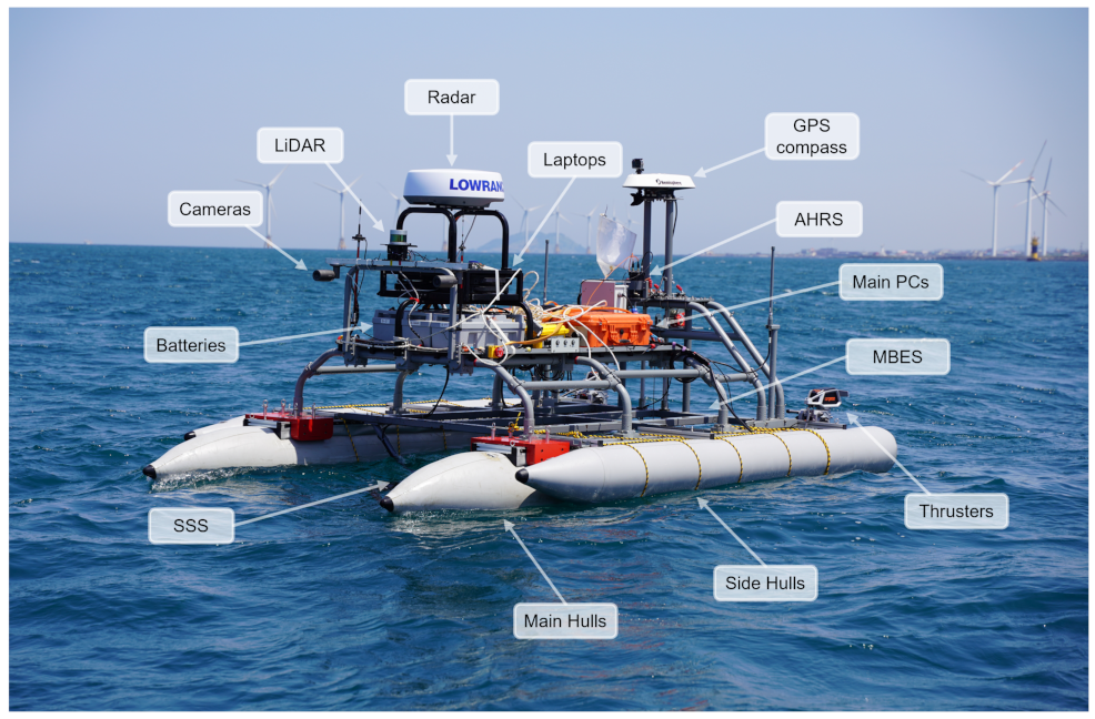
2.1. Hardware System
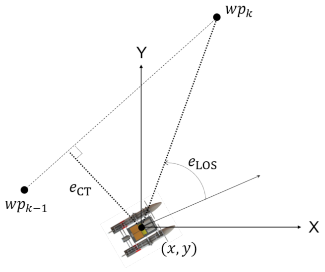
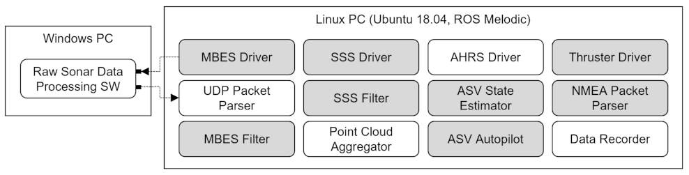
2.2. Control Architecture
3. Consistent Mapping
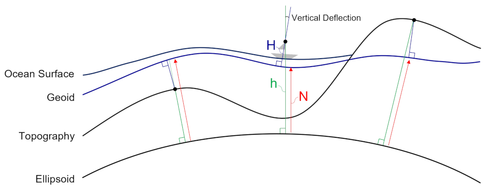
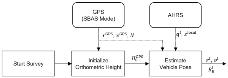
3.1. Motion Estimation
3.2. MBES Mapping
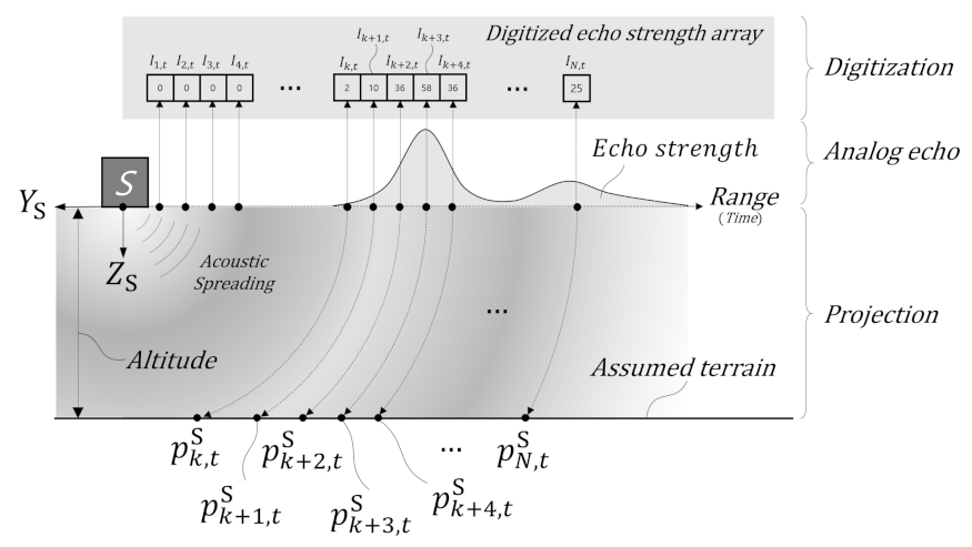
3.3. SSS Mapping
4. Experiments
4.1. Experimental Setup
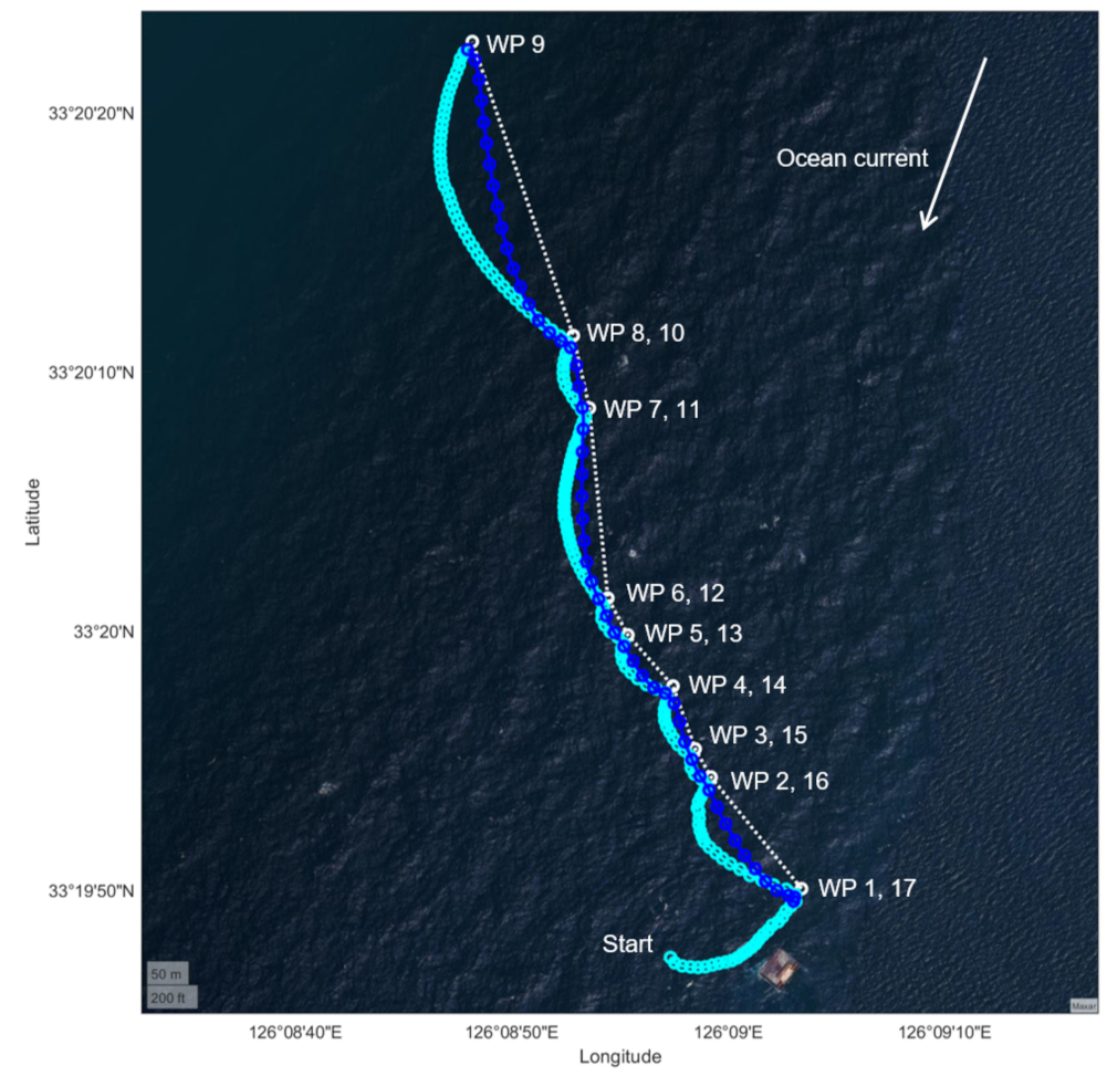
4.2. Waypoint Trakcing Results
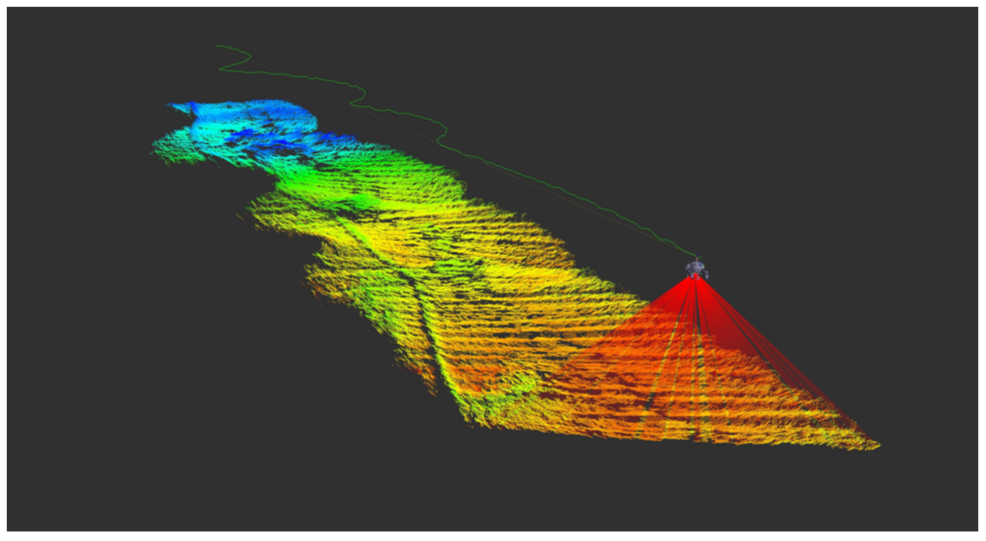
4.3. MBES Mapping Results
4.4. SSS Mapping Results
5. Conclusions
Author Contributions
Funding
Institutional Review Board Statement
Informed Consent Statement
Data Availability Statement
Acknowledgments
Conflicts of Interest
References
- Schiaretti, M.; Chen, L.; Negenborn, R.R. Survey on Autonomous Surface Vessels: Part I-A New Detailed Definition of Autonomy Levels. In Computational Logistics; Bektaş, T., Coniglio, S., Martinez-Sykora, A., Voß, S., Eds.; Springer: Berlin/Heidelberg, Germany, 2017; pp. 219–233. [Google Scholar]
- Schiaretti, M.; Chen, L.; Negenborn, R.R. Survey on Autonomous Surface Vessels: Part II-Categorization of 60 Prototypes and Future Applications. In Computational Logistics; Bektaş, T., Coniglio, S., Martinez-Sykora, A., Voß, S., Eds.; Springer: Berlin/Heidelberg, Germany, 2017; pp. 234–252. [Google Scholar]
- Kum, B.C.; Shin, D.H.; Lee, J.H.; Moh, T.; Jang, S.; Lee, S.Y.; Cho, J.H. Monitoring Applications for Multifunctional Unmanned Surface Vehicles in Marine Coastal Environments. J. Coast. Res. 2018, 85, 1381–1385. [Google Scholar] [CrossRef]
- Cost Reduction in E&P, IMR, and Survey Operations Using Unmanned Surface Vehicles. In OTC Offshore Technology Conference; 2018. Available online: https://onepetro.org/OTCONF/proceedings-pdf/18OTC/4-18OTC/D041S054R004/1193771/otc-28707-ms.pdf (accessed on 16 January 2022).
- Carlson, D.F.; Fürsterling, A.; Vesterled, L.; Skovby, M.; Pedersen, S.S.; Melvad, C.; Rysgaard, S. An affordable and portable autonomous surface vehicle with obstacle avoidance for coastal ocean monitoring. HardwareX 2019, 5, e00059. [Google Scholar] [CrossRef]
- Nicholson, D.P.; Michel, A.P.M.; Wankel, S.D.; Manganini, K.; Sugrue, R.A.; Sandwith, Z.O.; Monk, S.A. Rapid Mapping of Dissolved Methane and Carbon Dioxide in Coastal Ecosystems Using the ChemYak Autonomous Surface Vehicle. Environ. Sci. Technol. 2018, 52, 13314–13324. [Google Scholar] [CrossRef] [PubMed]
- Karapetyan, N.; Moulton, J.; Rekleitis, I. Dynamic Autonomous Surface Vehicle Control and Applications in Environmental Monitoring. In Proceedings of the OCEANS 2019 MTS/IEEE SEATTLE, Seattle, WA, USA, 27–31 October 2019; pp. 1–6. [Google Scholar] [CrossRef]
- Yan, R.; Pang, S.; Sun, H.; Pang, Y. Development and missions of unmanned surface vehicle. J. Mar. Sci. Appl. 2010, 9, 451–457. [Google Scholar] [CrossRef]
- Han, J.; Cho, Y.; Kim, J. Coastal SLAM With Marine Radar for USV Operation in GPS-Restricted Situations. IEEE J. Ocean. Eng. 2019, 44, 300–309. [Google Scholar] [CrossRef]
- Xiao, X.; Dufek, J.; Woodbury, T.; Murphy, R. UAV assisted USV visual navigation for marine mass casualty incident response. In Proceedings of the 2017 IEEE/RSJ International Conference on Intelligent Robots and Systems (IROS), Vancouver, BC, Canada, 24–28 September 2017; pp. 6105–6110. [Google Scholar] [CrossRef]
- Jorge, V.A.M.; Granada, R.; Maidana, R.G.; Jurak, D.A.; Heck, G.; Negreiros, A.P.F.; dos Santos, D.H.; Gonçalves, L.M.G.; Amory, A.M. A Survey on Unmanned Surface Vehicles for Disaster Robotics: Main Challenges and Directions. Sensors 2019, 19, 702. [Google Scholar] [CrossRef] [PubMed] [Green Version]
- Pu, H.; Liu, Y.; Luo, J.; Xie, S.; Peng, Y.; Yang, Y.; Yang, Y.; Li, X.; Su, Z.; Gao, S.; et al. Development of an Unmanned Surface Vehicle for the Emergency Response Mission of the ‘Sanchi’ Oil Tanker Collision and Explosion Accident. Appl. Sci. 2020, 10, 2704. [Google Scholar] [CrossRef] [Green Version]
- Capperucci, R.; Kubicki, A.; Holler, P.; Bartholomä, A. Sidescan sonar meets airborne and satellite remote sensing: Challenges of a multi-device seafloor classification in extreme shallow water intertidal environments. Geo-Mar. Lett. 2020, 40, 117–133. [Google Scholar] [CrossRef] [Green Version]
- Kampmeier, M.; van der Lee, E.M.; Wichert, U.; Greinert, J. Exploration of the munition dumpsite Kolberger Heide in Kiel Bay, Germany: Example for a standardised hydroacoustic and optic monitoring approach. Cont. Shelf Res. 2020, 198, 104108. [Google Scholar] [CrossRef]
- Pydyn, A.; Popek, M.; Kubacka, M.; Janowski, Ł. Exploration and reconstruction of a medieval harbour using hydroacoustics, 3-D shallow seismic and underwater photogrammetry: A case study from Puck, southern Baltic Sea. Archaeol. Prospect. 2021, 28, 527–542. [Google Scholar] [CrossRef]
- Petillot, Y.; Reed, S.; Bell, J. Real time AUV pipeline detection and tracking using side scan sonar and multi-beam echo-sounder. In Proceedings of the OCEANS ’02 MTS/IEEE, Biloxi, MI, USA, 29–31 October 2002; pp. 217–222. [Google Scholar] [CrossRef]
- DeKeyzer, R.; Byrne, J.; Case, J.; Clifford, B.; Simmons, W. A comparison of acoustic imagery of sea floor features using a towed side scan sonar and a multibeam echo sounder. In Proceedings of the OCEANS ’02 MTS/IEEE, Biloxi, MI, USA, 29–31 October 2002; pp. 1203–1211. [Google Scholar] [CrossRef]
- Barkby, S.; Williams, S.; Pizarro, O.; Jakuba, M. An efficient approach to bathymetric SLAM. In Proceedings of the 2009 IEEE/RSJ International Conference on Intelligent Robots and Systems, St. Louis, MO, USA, 10–15 October 2009; pp. 219–224. [Google Scholar] [CrossRef]
- Thompson, D.; Caress, D.; Paull, C.; Clague, D.; Thomas, H.; Conlin, D. MBARI mapping AUV operations: In the Gulf of California. In Proceedings of the 012 Oceans, Hampton Roads, VA, USA, 14–19 October 2012; pp. 1–5. [Google Scholar] [CrossRef]
- Fezzani, R.; Zerr, B.; Mansour, A.; Legris, M.; Vrignaud, C. Fusion of Swath Bathymetric Data: Application to AUV Rapid Environment Assessment. IEEE J. Ocean. Eng. 2019, 44, 111–120. [Google Scholar] [CrossRef]
- Rusu, R.B.; Marton, Z.C.; Blodow, N.; Dolha, M.; Beetz, M. Towards 3D Point cloud based object maps for household environments. Robot. Auton. Syst. 2008, 56, 927–941. [Google Scholar] [CrossRef]
- Quigley, M.; Gerkey, B.; Conley, K.; Faust, J.; Foote, T.; Leibs, J.; Berger, E.; Wheeler, R.; Ng, A. ROS: An open-source Robot Operating System. In Proceedings of the IEEE International Conference on Robotics and Automation (ICRA), Kobe, Japan, 12–17 May 2009. [Google Scholar]


| Item | Description |
|---|---|
| Dimension | 4.1 × 2.5 × 2.0 (L × W × H) m |
| Platform weight | 400 kg |
| Payload | up to 300 kg |
| Batteries | Lithium battery (25.9 VDC/ 104 Ah) × 3 |
| Propulsive power | 5 HP × 2 |
| Max. propeller speed | 1300 rpm |
| Speed | up to 6.35 knots |
| Endurance | 8 h @ 3 knots |
| Wireless Comm. | up to 1 km |
| Motion sensors | GPS compass (Hemisphere V113) |
| Mapping sensors | AHRS (Advanced Navigation Spatial FOG) |
| MBES (Imagenex 837B Delta T 260 kHz) | |
| SSS (Klein UUV3500 450/900 kHz) |
Publisher’s Note: MDPI stays neutral with regard to jurisdictional claims in published maps and institutional affiliations. |
© 2022 by the authors. Licensee MDPI, Basel, Switzerland. This article is an open access article distributed under the terms and conditions of the Creative Commons Attribution (CC BY) license (https://creativecommons.org/licenses/by/4.0/).
Share and Cite
Jung, J.; Lee, Y.; Park, J.; Yeu, T.-K. Multi-Modal Sonar Mapping of Offshore Cable Lines with an Autonomous Surface Vehicle. J. Mar. Sci. Eng. 2022, 10, 361. https://doi.org/10.3390/jmse10030361
Jung J, Lee Y, Park J, Yeu T-K. Multi-Modal Sonar Mapping of Offshore Cable Lines with an Autonomous Surface Vehicle. Journal of Marine Science and Engineering. 2022; 10(3):361. https://doi.org/10.3390/jmse10030361
Chicago/Turabian StyleJung, Jongdae, Yeongjun Lee, Jeonghong Park, and Tae-Kyeong Yeu. 2022. "Multi-Modal Sonar Mapping of Offshore Cable Lines with an Autonomous Surface Vehicle" Journal of Marine Science and Engineering 10, no. 3: 361. https://doi.org/10.3390/jmse10030361
APA StyleJung, J., Lee, Y., Park, J., & Yeu, T.-K. (2022). Multi-Modal Sonar Mapping of Offshore Cable Lines with an Autonomous Surface Vehicle. Journal of Marine Science and Engineering, 10(3), 361. https://doi.org/10.3390/jmse10030361