An Initial Field Intelligent Correcting Algorithm for Numerical Forecasting Based on Artificial Neural Networks under the Conditions of Limited Observations: Part I—Focusing on Ocean Temperature

Abstract

For the numerical forecasting of ocean temperature, the effective fusion of observations and the initial field under the conditions of limited observations has always been a significant problem. Traditional data assimilation methods cannot make full use of limited observations to correct the initial field. In order to obtain an optimal initial field with limited observations, this study proposed an intelligent correcting (IC) algorithm based on artificial neural networks (ANNs). The IC algorithm can fully mine the correlation laws between the grid points using historical data, and this process essentially replaces the estimation of background error covariance in traditional data assimilation methods. Experimental results show that the IC algorithm can lead to superior forecasting accuracy, with a lower root mean square error (around 0.7 °C) and higher coefficient of determination (0.9934) relative to the optimal interpolation method. Through the IC algorithm, the largest reduction in mean forecasting error can reach around −0.5 °C and the maximum percentage decline in mean forecasting error can reach 30% compared with the original numerical forecasting results. Therefore, the experiments validate that the IC algorithm can effectively correct the initial field under the conditions of limited observations.

1. Introduction

Ocean temperature has important impacts on sonar detection accuracy, hydroacoustic communication efficiency, submarine navigation safety and so on. Accurate ocean temperature forecasting is beneficial to marine activities.

The approaches for ocean temperature forecasting can be divided into two categories, including numerical models and data-driven models. Numerical models are based on dynamic equations, while data-driven models are based on statistical laws of historical data. The forecasting approach of data-driven models has seen rapid progress in recent years [1,2,3,4,5,6]. However, numerical models are still the mainstream approach for ocean–atmosphere forecasting [7,8,9,10,11].

Initial field correcting is the key step in numerical forecasting systems. Compared with the truth value, the initial field of a numerical model has errors that need to be corrected. Currently, the initial field correcting approach usually adopts data assimilation methods. Data assimilation uses observations to reconstruct ocean–atmosphere data and provide the best estimation of the initial field for numerical models. Lewis Fry Richardson carried out the first data assimilation in meteorology [12]. With the development of Earth numerical forecasting technology, data assimilation gradually began to be applied in oceanographic forecasting [13,14,15,16,17]. Generally, traditional data assimilation methods, including optimal interpolation (OI) [18], three-dimensional variation data assimilation (3D-Var) [19], four-dimensional variation data assimilation (4D-Var) [20], ensemble Kalman filter (ENKF) [21] and ensemble adjustment Kalman filter (EAKF) [22], are all effective approaches for correcting the initial field of numerical models. However, the effect of traditional assimilation methods is greatly affected by the spatial distribution of observations. In the case of sufficient observation data and optimal distribution, traditional data assimilation methods can achieve good results. However, when the observations are limited, traditional data assimilation methods are less effective. The decline of correcting effects is caused by a lack of effective information.

Limited observations mean that the quantity of observations is scarce and the spatial distribution is not optimal. Limited observations, including some randomly distributed Argo buoys and ship survey data, are very common in practical applications. Making full use of limited observations can effectively improve the numerical forecasting accuracy.

In the process of traditional data assimilation, limited observations reduce the credibility of correlations between observation points and other grid points. In order to improve the correcting accuracy for the initial field, it is necessary to use historical data to supplement the effective information needed in the correcting process. Artificial neural networks (ANNs) are powerful tools for capturing historical laws. In recent years, ANNs have been widely used in the fields of computer vision, speech recognition, physics, chemistry and biology [23,24,25,26]. Moreover, ANNs have achieved notable success in geosciences [27,28,29,30,31,32]. In view of the advantages of ANNs, ANNs are expected to improve the correcting accuracy for the initial field under the conditions of limited observations.

In order to address the restrictions of limited observations in ocean temperature forecasting, this study proposes an intelligent correcting (IC) algorithm based on ANNs that are used for obtaining an optimal initial field. The IC algorithm can fully mine correlation laws between the grid points using historical data, and this process essentially replaces the estimation of background error covariance in traditional data assimilation methods.

In this study, the northeast of the South China Sea is selected as the study area and a series of Argo buoys are used to test the forecasting accuracy. Moreover, computer simulations and observation data analyses are performed by considering admissible levels of error in the work.

The remainder of this paper is organized as follows. Section 2 describes the numerical forecasting model and explains the principle of the IC algorithm. Section 3 describes the experimental details. Section 4 presents the experimental results. A discussion is given in Section 5 and a summary is given in Section 6.

2. Methods

2.1. Numerical Forecasting Model

In recent years, numerical models have seen great progress, including global models and regional models. However, a single model cannot accurately describe the whole physical process of ocean–atmosphere change. Coupled models are more scientific than a single model in dynamics and physics and they have gradually become the mainstream in the field of numerical forecasting.

The numerical model of this study is the Coupled Ocean–Atmosphere–Wave–Sediment Transport (COAWST) modeling system [33], a regional ocean–atmosphere–wave coupling numerical model that describes the motion processes of the atmosphere, ocean and waves. Relevant studies show that the COAWST has reliable performance [34,35,36].

The COAWST modeling system comprises several components, which include an ocean model, the Regional Ocean Modeling System (ROMS) [37]; an atmosphere model, Weather Research and Forecasting (WRF) [38]; and a wave model, Simulating Waves Nearshore (SWAN) [39].

ROMS is a free-surface oceanic model. The horizontal grid is the Arakawa C grid. ROMS uses a stretched terrain-following coordinate in the vertical direction [37]. ROMS can provide forecasting data of temperature, salinity, current and other variables.

WRF is a non-hydrostatic and quasi-compressible atmospheric model. WRF uses the Arakawa C grid in the horizontal direction and terrain-following, hydrostatic-pressure vertical coordinate [38]. WRF can provide forecasting data of wind, surface pressure, surface sensible and latent heat fluxes, longwave and shortwave radiative fluxes, air temperature, dew point, relative humidity and precipitation on a sigma-pressure vertical coordinate grid.

SWAN is a wave model that can simulate the generation and propagation of wind waves by solving the spectral density evolution equation and action balance equation [39]. Moreover, SWAN can provide forecasting data of wave height, wave length, wave direction and other variables.

In the COAWST modeling system, ROMS provides the sea surface temperature to WRF, and WRF provides winds, atmospheric surface temperature, atmospheric pressure, precipitation, relative humidity, cloud fraction, shortwave and longwave to ROMS. ROMS provides surface currents, free surface elevation and bathymetry to SWAN, and SWAN provides wave height, wave length, wave direction, percent wave breaking, wave energy dissipation, surface and bottom periods and bottom orbital velocity to ROMS. WRF provides winds to SWAN, and SWAN provides wave height and wave length to WRF. More details about COAWST can be found in Warner et al. [33].

2.2. IC Algorithm

ANNs have powerful functions of fitting capabilities for nonlinear mapping [23,32]. ANNs are made up of a multitude of neurons connected with adjustable weights and are capable of autonomous learning through backpropagation algorithms. An ANN consists of an input layer, multiple hidden layers and an output layer. When there are enough hidden layers and neurons in an ANN, it can fit complex nonlinear mappings [40]. The form of neuron connection is displayed in Figure 1.

Suppose that there are n neurons in the k layer. $x_i^{\left(k\right)}$ is the i-th neuron in the k layer. $w_{ij}^{\left(k\right)}$ is the weight parameter of the k layer. Let $x_j^{\left(k+1\right)}$ be the output of the j-th neuron in the k + 1 layer, and $b_j^{\left(k\right)}$ is the bias parameter of the j-th neuron in the k + 1 layer about the k layer. ${\sigma }^{\left(k+1\right)}$ is the nonlinear activation function in the k + 1 layer. Then, the following formula can be obtained:

$$x_j^{\left(k+1\right)}={\sigma }^{\left(k+1\right)}\left({\displaystyle \sum }_{i=1}^n{w}_{ij}^{\left(k\right)}{x}_i^{\left(k\right)}+b_j^{\left(k\right)}\right),$$

(1)

Through the connected neurons, the information flow is nested to form a nonlinear mapping function:

$$y_j^{\left(p\right)}={\eta }_j\left(x_1^{\left(1\right)},x_2^{\left(1\right)},\cdots \cdots x_n^{\left(1\right)}\right),$$

(2)

where $y_j^{\left(p\right)}$ is the received information of the j-th neuron in the p layer. ${\eta }_j$ is the nonlinear mapping function of the j-th neuron in the p layer.

Equation (2) indicates that the signal of any one neuron in the output layer will create a nonlinear mapping with all signals in the input layer. In order to mine the laws of sample data and label data through an ANN, we put the sample data into the input layer and the output signals can be obtained from the output layer after the calculation of the hidden layers. The output signals would be compared with the label data and the weights of the ANN are adjusted by backpropagation [40]. After a suitable number of iterations, the trained ANN can fit the laws of sample data and label data when the output signals are close to the label data.

Based on the property that ANNs can mine the laws of sample data and label data, we consider applying it to initial field correcting. The key of initial field correcting is to extend the observation information to other grid points without observation information. Under the conditions of limited observations, we should use the patterns embedded in historical data to supplement the useful information needed in the correcting process. When we obtain observations of some points, the observational values of these points must differ from the values of the background field (the original initial field), and we can define this deviation as the observation increment. Our goal is to use the currently known observation increments to estimate the observation increments for all grid points, so that the obtained entire observation increments field can be used to correct the initial field to be closer to the true value (here, the observations are approximated as true values).

In traditional assimilation methods, background error covariance is used to represent the correlation between observation points and non-observation points. Now, we can use ANNs to mine the correlations between these grid points in historical data. Since ANNs have nonlinear mapping functions, ANNs can more adequately find correlations between these grid points than background error covariance.

Thus, we propose the IC algorithm based on ANNs. The neural network form adopted in this study is fully connected, and the following ANNs all refer to fully connected ANNs. The overall flowchart of the IC algorithm is shown in Figure 2.

The detailed steps are described below.

(1)

Take out the location information of the grid points that have observations. According to the location information, the grid points are marked in the initial field and in the historical data at the corresponding locations.

(2)

The temperature of the marked grid points in the historical data at different times minus the temperature of the marked grid points in the initial field is used to obtain the set of training samples. The temperature of all the grid points in the historical data at different times minus the temperature of all the grid points in the initial field is used to obtain the set of training labels.

(3)

Build the ANN and train it with the obtained samples and labels.

(4)

The observation temperature minus the temperature of corresponding marked grid points in the initial field is used to obtain the observation increment.

(5)

Input the observation increments into the trained ANN to obtain the entire analysis increments field.

(6)

Add the entire analysis increment field to the initial field to obtain the optimal initial field

(7)

Put the optimal initial field into the numerical model to produce more accurate forecasting results.

The essence of the IC process is to use historical data for the spatial extension of observation information. ANNs are used to establish the nonlinear mapping correlation between the observation increment and the entire increment field. ANNs can learn the correlation laws between observation points and other grid points from historical data, which are difficult for humans to discover. The application of ANNs can greatly improve the utilization efficiency of historical data and observations relative to traditional data assimilation methods.

3. Experiment

3.1. Evaluation Criteria

This study uses limited observations to correct the initial field, but it is very difficult to obtain enough observations at the same time for testing the correcting effect. Therefore, this experiment evaluates the correcting effect of the initial field by testing the error of forecasting results. Since the OI method has been widely and effectively applied in the general data assimilation, we used the OI method for the experimental control groups under the same conditions. In the control experiment, only the initial field was different and the other settings were unchanged. Thus, the correcting method with the smallest forecasting error indicates that the initial field error is the smallest.

This experiment used single random observations at different times to judge the forecasting errors through statistics. The absolute error (AE) and mean absolute error (MAE) were used to evaluate the forecasting error at different depths. The root mean square error (RMSE) and coefficient of determination (R²) were used to evaluate the overall correcting effect. The equations of AE, MAE, RMSE and R² are as follows [41]:

$$AE=\left|m-a\right|,$$

(3)

$$MAE=\frac{{{\displaystyle \sum }}_{i=1}^d\left|m_i-a_i\right|}{d},$$

(4)

$$RMSE=\sqrt{\frac{{{\displaystyle \sum }}_{i=1}^p{\left(m_i-a_i\right)}^2}{p}},$$

(5)

$$R^2=1-\frac{{{\displaystyle \sum }}_{i=1}^p{\left(a_i-m_i\right)}^2}{{{\displaystyle \sum }}_{i=1}^p{\left(a_i-a_{mean}\right)}^2},$$

(6)

where $m$ is the forecasting results, $a$ is the observational data, $d$ is the number of used Argo buoys for evaluation, $p$ is the number of all observation data, and $a_{mean}$ is the mean value of all observation data.

3.2. Data Collection

In this study, the atmosphere data come from FNL reanalysis data. Available online: https://rda.ucar.edu/datasets/ds083.2/ (accessed on 1 January 2020). FNL reanalysis data provide the initial field and boundary field of WRF. The ocean data come from HYCOM reanalysis data. Available online: https://www.hycom.org/dataserver/ (accessed on 2 January 2020). HYCOM reanalysis data provide the initial field and boundary field of ROMS. A series of Argo buoys are used as observation data, which come from the Chinese Argo Real-time Data Center. Available online: http://www.argo.org.cn/data/argo.php/ (accessed on 10 October 2019).

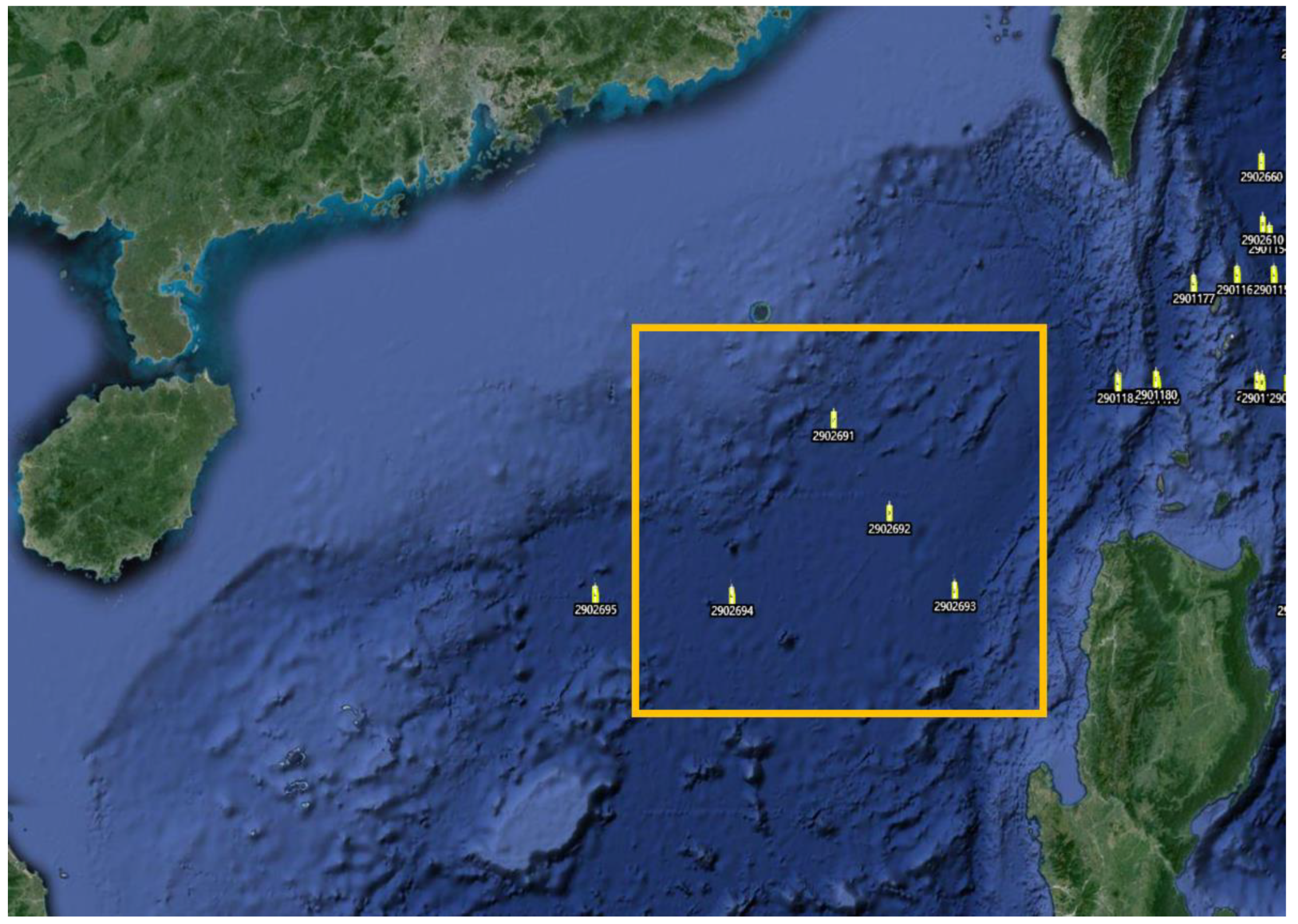
As there are a considerable number of Argo buoys in the northeast of the South China Sea that have good experimental conditions, the northeast of the South China Sea is chosen as the experimental area. The Argo position is shown in Figure 3 and the selected experimental Argo buoys are in the orange square.

3.3. Experimental Scheme

The Argo data provide 2000 m temperature profiles every 5 days and then multiple Argo data can compose a series of continuous observation data. The experimental area ranges from 112° E to 124° E and 13.5° N to 23° N.

In order to test the correcting effect under different limited observation distributions, the experiment is divided into four groups. The Argo spatial distribution of the four experimental groups is shown in Figure 4. The observations of blue points are used to correct the initial field, and the observations of purple points are used to test the forecasting error. Figure 4a is the Argo spatial distribution of Experiment 1, and the forecast period is 2016.9.12–2016.9.26. Figure 4b is the Argo spatial distribution of Experiment 2, and the forecast period is 2016.9.15–2016.9.29. Figure 4c is the Argo spatial distribution of Experiment 3, and the forecast period is 2016.9.13–2016.9.27. Figure 4d is the Argo spatial distribution of Experiment 4, and the forecast period is 2016.9.17–2016.10.01.

3.4. Main Parameter Settings

The ocean model resolution was set to 9 km and the horizontal grid size was set to 150 × 120. The vertical grid was set to 20 layers with a stretched terrain-following coordinate [37] (theta_s = 4.0, theta_b = 0.1). The historical data for ANN training use 10-year data that come from HYCOM.

Pytorch was used as an ANN tool in this study. Available online: https://pytorch.org/ (accessed on 9 September 2020). The ANNs used fully connected networks and the activation function adopted was ReLU. The hidden layer was set to two layers and the number of neurons in the hidden layers was 48. The number of neurons in the input layer was the number of observations. The number of neurons in the output layer was 18,000. The initial learning rate was 0.01 and the learning rate could be adaptively reduced. The epoch value was 500. The optimizer was Adam, and the loss function was MSELoss. To quickly stabilize the model, the increment field was smoothed. The smoothing tool was cv2 and the function adopted was GaussianBlur. The Gaussian kernel size was 5 × 5, and the standard deviation was set to 0.9.

4. Results

The 0, 50, 100, 200, 500 and 1000 m ocean depths were sampled to present the forecasting results of the surface layer, thermocline, and deep layer. Figure 5, Figure 6, Figure 7 and Figure 8 are the temperature forecasting errors of different experimental groups.

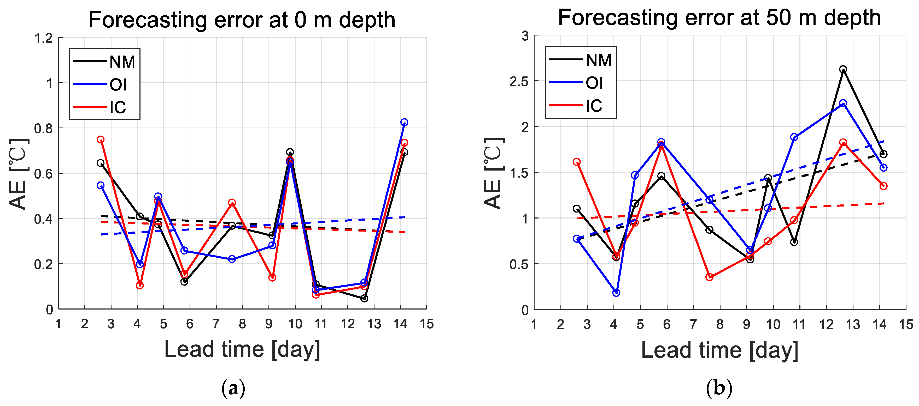
Figure 5 is the temperature forecasting error of Experiment 1. From Figure 5a, it can be found that the forecasting errors of the NM, the OI and the IC are very close, which indicates that the correcting effect of the OI and the IC is not obvious on the surface. The overall forecasting error of the IC at other depths is lower than that of NM through regression analysis, which shows that the IC algorithm has effectively corrected the initial field at other depths. At the depths of 50, 200 and 1000 m, the OI increases the forecasting error to a certain extent, while the performance of the IC is relatively stable.

Figure 6 is the temperature forecasting error of Experiment 2. The results of Experiment 2 show that the correcting effect of the OI is better than that of the IC on the surface layer. However, in the thermocline of 50, 100 and 200 m, the correcting effect of the IC is better than that of the OI. At the depths of 500 and 1000 m, both the OI and the IC increase the forecasting error.

Figure 7 is the temperature forecasting error of Experiment 3. The results of Experiment 3 show that the correcting effects of the OI and the IC are not obvious on the surface or at 1000 m depth. The correcting effect of the OI and the IC is obvious at 50 m depth. Moreover, the correcting effect of the IC is better than that of the OI. The correcting effect of the OI and the IC is close at 100 m depth. At the depths of 200 and 500 m, the correcting effect of the IC is better than that of the OI.

Figure 8 is the temperature forecasting error of Experiment 4. The results of Experiment 4 show that at the surface and at the depths of 50 and 500 m, the correcting effect of the OI and the IC is not obvious. At the depths of 100 and 200 m, the overall forecasting error of the IC is lower than that of the NM and better than that of the OI. At 1000 m depth, both the IC and the OI increase the forecasting error.

It can be seen from the forecasting error graph that the IC algorithm has better stability for thermocline correcting efficiency. At the surface and deep layers, the forecasting error may be increased. The overall performance of the OI is good, but it is sometimes unstable, and the forecasting error will increase in some layers. This may be caused by a lack of observations under limited observation conditions.

Table 1. MAE.

Experiment Group	Method	0 m	50 m	100 m	200 m	500 m	1000 m
Experiment 1	NM	0.3763	1.2164	1.2111	0.8322	0.3121	0.1849
	OI	0.3656	1.2857	0.9057	0.9008	0.3043	0.2143
	IC	0.3630	1.0741	0.8035	0.6806	0.2555	0.1606
Experiment 2	NM	0.4400	0.9588	1.4145	0.6916	0.3722	0.1345
	OI	0.4050	1.1365	1.4425	0.7733	0.4182	0.1550
	IC	0.4006	0.9424	1.2166	0.5489	0.3865	0.1768
Experiment 3	NM	0.3709	1.2869	1.5495	0.8654	0.2991	0.1721
	OI	0.3591	1.1009	1.1028	0.8511	0.3058	0.1632
	IC	0.4024	0.9756	1.0841	0.7200	0.2588	0.1648
Experiment 4	NM	0.3186	1.0201	1.4571	0.6952	0.3169	0.1573
	OI	0.3483	1.1156	1.2707	0.6535	0.2997	0.1657
	IC	0.3308	0.9826	1.1949	0.5766	0.3203	0.1871

shows the MAE of the four experimental groups. The MAE can represent the mean forecasting error. It can be seen from Table 1 that for the thermocline with large errors, the IC algorithm has better correcting effects. At the surface layer and deep layers with small errors, neither the OI nor the IC show obvious advantages. Compared with the NM results, the largest reduction in mean forecasting error can reach around −0.5 °C, which occurs at the depth of 100 m in Experiment 3, and the maximum percentage decline in mean forecasting error can reach 30%.

Table 2. RMSE and R².

Evaluation Criteria	Method	Experiment 1	Experiment 2	Experiment 3	Experiment 4	Mean
RMSE	NM	0.7945	0.7888	0.9446	0.8411	0.8423
	OI	0.7454	0.8097	0.8106	0.8069	0.7932
	IC	0.6851	0.7208	0.7758	0.7401	0.7305
R2	NM	0.9921	0.9923	0.9889	0.9911	0.9912
	OI	0.9931	0.9919	0.9918	0.9918	0.9922
	IC	0.9942	0.9935	0.9925	0.9931	0.9934

shows the RMSE and R² of the four experimental groups. It can be seen from Table 2 that the RMSE of IC can reach around 0.7 ℃; the percentage reduction is around 13% and 8%, respectively, relative to NM and OI. The mean R² of IC can reach 0.9934; the improvement is 0.0022 and 0.0012, respectively, relative to NM and OI. Overall, the correcting effects of the IC algorithm are better than those of the OI method under the conditions of limited observations.

5. Discussion

Through the experiments under different conditions of observational distributions, it can be found that at the depths of 50, 100 and 200 m, the IC algorithm has significant advantages. Since the depths of 50, 100 and 200 m are mainly in the thermocline with large errors, this result indicates that the IC algorithm is effective for large errors. However, both the IC algorithm and the OI method have unstable correcting effects at the surface layer and the deep layer, which may be caused by limited correcting accuracy. As many sea surface observations have been assimilated into the original field that comes from HYCOM reanalysis data, the errors of sea surface temperature are generally small. The implementation of correcting algorithms on the sea surface may bring new disturbance errors. When the disturbance errors are greater than the original errors, the correcting algorithm will lose efficacy. Meanwhile, in the deep ocean, the error magnitude is usually small. When the disturbance errors caused by the correcting algorithm are greater than the original errors, the correcting algorithm will also lose efficacy. To improve the correcting accuracy, the number of observations needs to be increased. Since this study focuses on the correcting algorithm under the conditions of limited observations, for the initial field derived from the reanalysis data with small errors, the correcting algorithm may have reached the limit of correcting accuracy at the surface layer and deep layer.

The better performance of the IC algorithm in the thermocline is understandable. The role of background error covariance in traditional data assimilation methods is to spread the observation information to other grid points. Background error covariance is unable to obtain accurate values, and can only be approximated by statistical methods. The general methods of obtaining background error covariance are based on linear correlation assumptions and cannot calculate the nonlinear process, so the effective information of historical data is not fully mined. When the observations distribution is limited, the traditional data assimilation methods are less effective. The IC algorithm based on nonlinear mapping can make full use of historical data, and effectively diffuses the observation information to other grid points. Under the conditions of limited observations, the IC algorithm is a feasible and effective correcting method.

In addition, traditional data assimilation methods have some insurmountable defects. The background error covariance and the assimilation radius are difficult to determine. Traditional data assimilation methods use a lot of approximation and subjective experience, and it is difficult to achieve parameter optimization and parameter self-adaptation. Meanwhile, the IC algorithm can realize parameter self-adaptation, and the historical data can be automatically optimized through ANNs. In practical applications, the IC algorithm has more convenience, and is simple for novices to operate.

We have only performed a preliminary study on ocean temperature. There is still much work to be done to achieve a complete IC algorithm. Many problems remain to be solved. Below, we discuss some issues to be studied.

(1) The IC algorithm for all variables: This study only focuses on ocean temperature. The follow-up study will extend to ocean salinity, waves, current and wind. Then, the IC algorithm can be combined with the coupled data assimilation (CDA) technology to further improve the numerical forecasting accuracy.

(2) The IC algorithm based on multi-source observations: In this study, only scattered Argo observations are used. In the actual situation, all available observation data including satellite, buoys and other real-time ship survey data should be fully utilized to improve the forecasting accuracy.

(3) Expanding applications of the IC algorithm: The IC algorithm is expected to be applied in a larger range of numerical forecasting. The IC algorithm based on ANNs can be combined with traditional assimilation methods, or used as an effective supplement to traditional assimilation methods, applied in global models to improve the accuracy of climate prediction.

6. Conclusions

In this study, the feasibility of the IC algorithm based on ANNs is preliminarily demonstrated by ocean temperature forecasting. The results show that the IC algorithm can effectively improve the forecasting accuracy of ocean temperature for the northeast of the South China Sea. The IC algorithm can lead to superior forecasting accuracy, with a lower root mean square error (around 0.7 °C) and higher coefficient of determination (0.9934) relative to the optimal interpolation method. Furthermore, compared with the original numerical forecasting results, the IC algorithm can reduce the temperature forecasting error by up to 30%. Therefore, the experiments validate that the IC algorithm can effectively correct the initial field under the conditions of limited observations. The IC algorithm avoids the calculation of background error covariance of traditional data assimilations and achieves parameter self-adaptation ability. The IC algorithm maximizes the utilization of observations and history data. It has good stability and universality. Thus, the IC algorithm is a convenient and effective correcting method for the initial field of numerical models, thereby improving the forecasting accuracy of numerical models.

References

- Patil, K.; Deo, M.C. Prediction of daily sea surface temperature using efficient neural networks. Ocean Dyn. 2017, 67, 357–368. [Google Scholar] [CrossRef]
- Gavrilov, A.; Seleznev, A.; Mukhin, D.; Loskutov, E.; Feigin, A.; Kurths, J. Linear dynamical modes as new variables for data-driven ENSO forecast. Clim. Dyn. 2019, 52, 2199–2216. [Google Scholar] [CrossRef]
- Kim, K.S.; Lee, J.B.; Roh, M.I.; Han, K.M.; Lee, G.H. Prediction of Ocean Weather Based on Denoising Auto Encoder and Convolutional LSTM. J. Mar. Sci. Eng. 2020, 8, 805. [Google Scholar] [CrossRef]
- Zhang, Z.; Pan, X.L.; Jiang, T.; Sui, B.K.; Liu, C.X.; Sun, W.F. Monthly and Quarterly Sea Surface Temperature Prediction Based on Gated Recurrent Unit Neural Network. J. Mar. Sci. Eng. 2020, 8, 249. [Google Scholar] [CrossRef]
- Zheng, G.; Li, X.F.; Zhang, R.H.; Liu, B. Purely satellite data-driven deep learning forecast of complicated tropical instability waves. Sci. Adv. 2020, 6, eaba1482. [Google Scholar] [CrossRef]
- Zhang, X.Y.; Li, Y.Q.; Gao, S.; Ren, P. Ocean Wave Height Series Prediction with Numerical Long Short-Term Memory. J. Mar. Sci. Eng. 2021, 9, 514. [Google Scholar] [CrossRef]
- Pinardi, N.; Cavaleri, L.; Coppini, G.; De Mey, P.; Fratianni, C.; Huthnance, J.; Lermusiaux, P.F.J.; Navarra, A.; Preller, R.; Tibaldi, S. From weather to ocean predictions: An historical viewpoint. J. Mar. Res. 2017, 75, 103–159. [Google Scholar] [CrossRef][Green Version]
- Zalesny, V.; Agoshkov, V.; Shutyaev, V.; Parmuzin, E.; Zakharova, N. Numerical Modeling of Marine Circulation with 4D Variational Data Assimilation. J. Mar. Sci. Eng. 2020, 8, 503. [Google Scholar] [CrossRef]
- Roh, M.; Kim, H.S.; Chang, P.H.; Oh, S.M. Numerical Simulation of Wind Wave Using Ensemble Forecast Wave Model: A Case Study of Typhoon Lingling. J. Mar. Sci. Eng. 2021, 9, 475. [Google Scholar] [CrossRef]
- Karna, T.; Ljungemyr, P.; Falahat, S.; Ringgaard, I.; Axell, L.; Korabel, V.; Murawski, J.; Maljutenko, I.; Lindenthal, A.; Jandt-Scheelke, S.; et al. Nemo-Nordic 2.0: Operational marine forecast model for the Baltic Sea. Geosci. Model Dev. 2021, 14, 5731–5749. [Google Scholar] [CrossRef]
- Kattamanchi, V.K.; Viswanadhapalli, Y.; Dasari, H.P.; Langodan, S.; Vissa, N.; Sanikommu, S.; Rao, S.V.B. Impact of assimilation of SCATSAT-1 data on coupled ocean-atmospheric simulations of tropical cyclones over Bay of Bengal. Atmos. Res. 2021, 261, 105733. [Google Scholar] [CrossRef]
- Shuman, F.G. History of numerical weather prediction at the National Meteorological Center. Weather Forecast. 1989, 4, 286–296. [Google Scholar] [CrossRef]
- Robinson, A.R.; Carton, J.A.; Mooers, C.N.K.; Walstad, L.J.; Carter, E.F.; Rienecker, M.M.; Smith, J.A.; Leslie, W.G. A real-time dynamical forecast of ocean synoptic/mesoscale eddies. Nature 1984, 309, 781–783. [Google Scholar] [CrossRef]
- Robinson, A.R.; Leslie, W.G. Estimation and prediction of ocean eddy fields. Prog. Oceanogr. 1985, 14, 485–510. [Google Scholar] [CrossRef]
- Robinson, A.R.; Carton, J.A.; Pinardi, N.; Mooers, C.N.K. Dynamical forecasting and dynamical interpolation: An experiment in the California Current. Phys. Oceanogr. 1986, 16, 1561–1579. [Google Scholar] [CrossRef][Green Version]
- Ghil, M.; Malanotte-Rizzoli, P. Data assimilation in meteorology and oceanography. Adv. Geophys. 1991, 33, 141–266. [Google Scholar] [CrossRef]
- Edwards, C.A.; Moore, A.M.; Hoteit, I.; Cornuelle, B.D. Regional ocean data assimilation. Ann. Rev. Mar. Sci. 2015, 77, 21–42. [Google Scholar] [CrossRef]
- Michele, M.R.; Robert, N.M. Ocean data assimilation using optimal interpolation with a quasi-geostrophic model. J. Geophys. Res. Oceans 1991, 96, 15093–15103. [Google Scholar] [CrossRef][Green Version]
- Sasaki, Y. Some basic formalisms in numerical variational analysis. Mon. Weather Rev. 1970, 98, 875–883. [Google Scholar] [CrossRef]
- Le Dimet, F.X.; Talagrand, O. Variational algorithms for analysis and assimilation of meteorological observations: Theoretical aspects. Tellus 1986, 38, 97–110. [Google Scholar] [CrossRef]
- Evensen, G. Sequential data assimilation with a nonlinear quasi-geostrophic model using Monte Carlo methods to forecast error statistics. J. Geophys. Res. Oceans 1994, 99, 10143–10162. [Google Scholar] [CrossRef]
- Anderson, J.L. An ensemble adjustment Kalman filter for data assimilation. Mon. Weather Rev. 2001, 129, 2884–2903. [Google Scholar] [CrossRef]
- LeCun, Y.; Bengio, Y.; Hinton, G. Deep learning. Nature 2015, 521, 436–444. [Google Scholar] [CrossRef]
- Baldi, P.; Sadowski, P.; Whiteson, D. Searching for exotic particles in high-energy physics with deep learning. Nat. Commun. 2014, 5, 4308. [Google Scholar] [CrossRef] [PubMed]
- Schütt, K.T.; Arbabzadah, F.; Chmiela, S.; Muller, K.R.; Tkatchenko, A. Quantum-chemical insights from deep tensor neural networks. Nat. Commun. 2017, 8, 13890. [Google Scholar] [CrossRef] [PubMed]
- Alipanahi, B.; Delong, A.; Weirauch, M.T.; Frey, B.J. Predicting the sequence specificities of DNA- and RNA-binding proteins by deep learning. Nat. Biotechnol. 2015, 33, 831–838. [Google Scholar] [CrossRef]
- Jung, M.; Reichstein, M.; Ciais, P.; Seneviratne, S.; Sheffield, J.; Goulden, M.; Bonan, G.; Chen, J.; Cescatti, A.; De Jeu, R.; et al. Recent decline in the global land evapotranspiration trend due to limited moisture supply. Nature 2010, 467, 951–954. [Google Scholar] [CrossRef]
- Jung, M.; Reichstein, M.; Schwalm, C.R.; Huntingford, C.; Sitch, S.; Ahlström, A.; Arneth, A.; Camps-Valls, G.; Ciais, P.; Friedlingstein, P.; et al. Compensatory water effects link yearly global land CO2 sink changes to temperature. Nature 2017, 541, 516–520. [Google Scholar] [CrossRef]
- Bonan, G.B.; Lawrence, P.J.; Oleson, K.W.; Levis, S.; Jung, M.; Reichstein, M.; Lawrence, D.M.; Swenson, S.C. Improving canopy processes in the Community Land Model version 4 (CLM4) using global flux fields empirically inferred from FLUXNET data. Geophys. Res. Biogeosci. 2011, 116, G02014. [Google Scholar] [CrossRef]
- Anav, A.; Friedlingstein, P.; Beer, C.; Ciais, P.; Harper, A.; Jones, C.; Murray-Tortarolo, G.; Papale, D.; Parazoo, N.C.; Peylin, P.; et al. Spatiotemporal patterns of terrestrial gross primary production: A review. Rev. Geophys. 2015, 53, 785–818. [Google Scholar] [CrossRef]
- Landschützer, P.; Gruber, N.; Bakker, D.C.E.; Schuster, U.; Nakaoka, S.; Payne, M.R.; Sasse, T.P.; Zeng, J. A neural network-based estimate of the seasonal to inter-annual variability of the Atlantic Ocean carbon sink. Biogeosciences 2013, 10, 7793–7815. [Google Scholar] [CrossRef]
- Reichstein, M.; Camps-Valls, G.; Stevens, B.; Jung, M.; Denzler, J.; Carvalhais, N.; Prabhat. Deep learning and process understanding for data-driven Earth system science. Nature 2019, 566, 195–204. [Google Scholar] [CrossRef] [PubMed]
- Warner, J.C.; Armstrong, B.; He, R.; Zambon, J.B. Development of a Coupled Ocean-Atmosphere-Wave-Sediment Transport (COAWST) modeling system. Ocean Model. 2010, 35, 230–244. [Google Scholar] [CrossRef]
- Liu, N.; Ling, T.J.; Wang, H.; Zhang, Y.F.; Gao, Z.Y.; Wang, Y. Numerical simulation of Typhoon Muifa (2011) using a Coupled Ocean-Atmosphere-Wave-Sediment Transport (COAWST) modeling system. J. Ocean Univ. 2015, 14, 199–209. [Google Scholar] [CrossRef]
- Zhang, C.; Hou, Y.J.; Li, J. Wave-current interaction during Typhoon Nuri (2008) and Hagupit (2008): An application of the coupled ocean-wave modeling system in the northern South China Sea. J. Oceanol. Limnol. 2018, 36, 663–675. [Google Scholar] [CrossRef]
- Zou, J.; Zhan, C.S.; Song, H.Q.; Hu, T.; Qiu, Z.J.; Wang, B.; Li, Z.Q. Development and Evaluation of a Hydrometeorological Forecasting System Using the Coupled Ocean-Atmosphere-Wave-Sediment Transport (COAWST) Model. Adv. Meteorol. 2021, 2021, 6658722. [Google Scholar] [CrossRef]
- Shchepetkin, A.F.; McWilliams, J.C. The Regional Ocean Modeling System: A split-explicit, free-surface, topography-following coordinates ocean model. Ocean Model. 2005, 9, 347–404. [Google Scholar] [CrossRef]
- Skamarock, W.C.; Klemp, J.B.; Dudhia, J.; Gill, D.O.; Barker, D.M.; Duda, M.G.; Huang, X.-Y.; Wang, W.; Powers, J.G. A Description of the Advanced Research WRF Version 3 (No. NCAR/TN-475+STR); University Corporation for Atmospheric Research: Boulder, CO, USA, 2008. [Google Scholar] [CrossRef]
- Booij, N.; Ris, R.C.; Holthuijsen, L.H. A third-generation wave model for coastal regions: 1. Model description and validation. J. Geophys. Res. Oceans 1999, 104, 7649–7666. [Google Scholar] [CrossRef]
- Schmidhuber, J. Deep learning in neural networks: An overview. Neural Netw. 2015, 61, 85–117. [Google Scholar] [CrossRef]
- Salem, H.; Kabeel, A.E.; El-Said, E.M.S.; Elzeki, O.M. Predictive modelling for solar power-driven hybrid desalination system using artificial neural network regression with Adam optimization. Desalination 2021, 522, 115411. [Google Scholar] [CrossRef]