
Trans-Media Kinematic Stability Analysis for Hybrid Unmanned Aerial Underwater Vehicle


Abstract
:1. Introduction
- (1)
- Based on the model of underwater vehicle maneuverability and the recent research results on air–water trans–media hydrodynamics, a simplified model for the air–water trans–media process is proposed.
- (2)
- Based on the Hurwitz method, the criterion of kinematic stability for the air–water trans–media motion of HAUVs is derived in this paper.
- (3)
- Based on the criterion proposed in this paper, the kinematic stability of an instance of HAUV, named Nezha, is analyzed.
2. Nezha System and Trans–Media Process
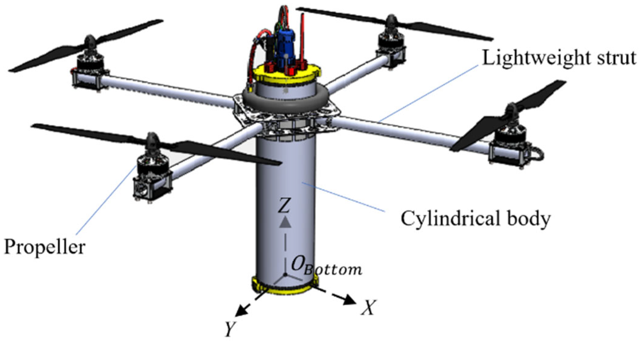
2.1. System Configuration
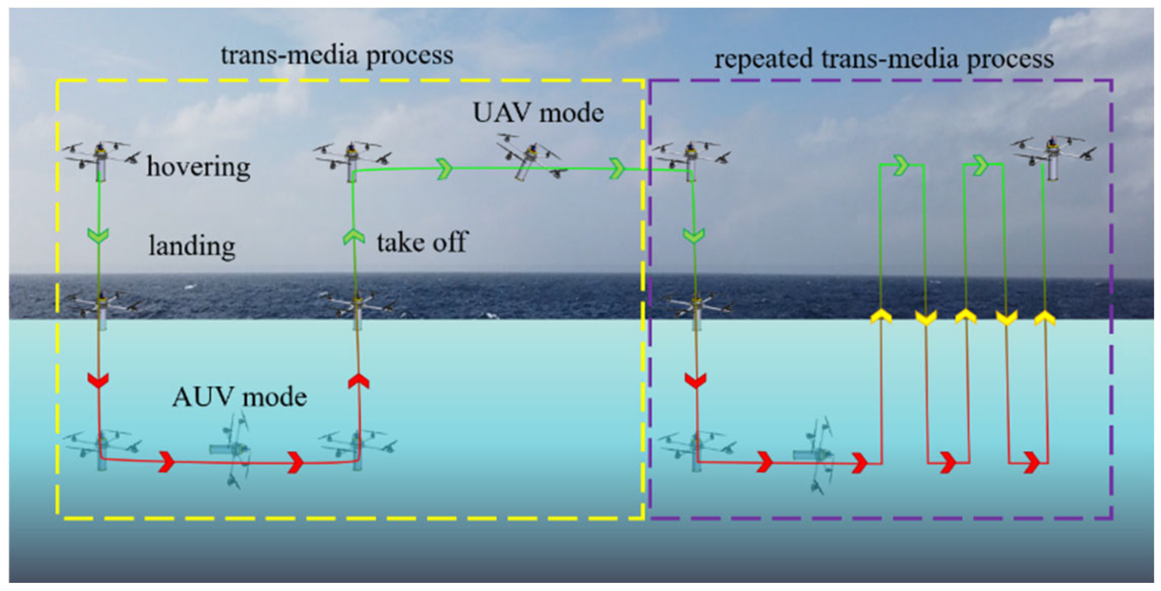
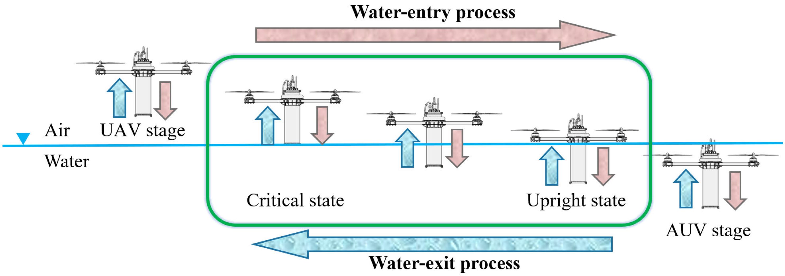
2.2. Trans–Media Motion Process
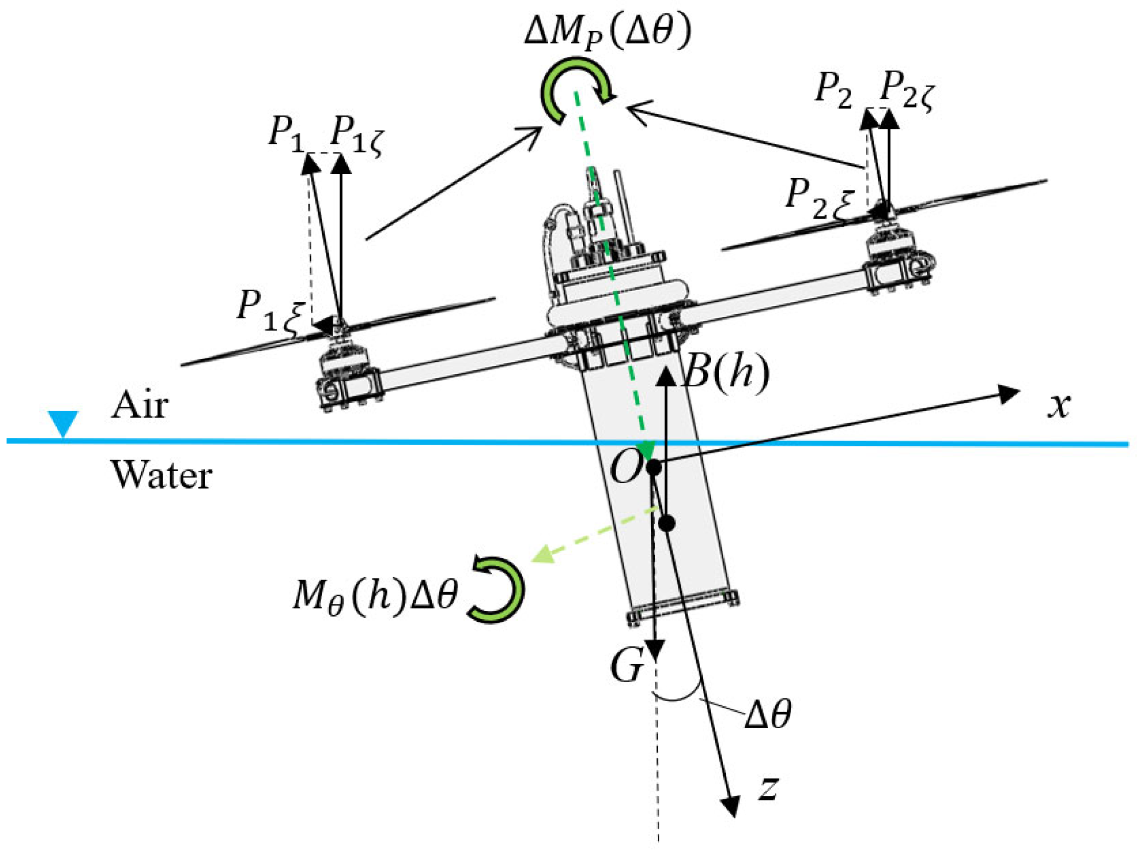
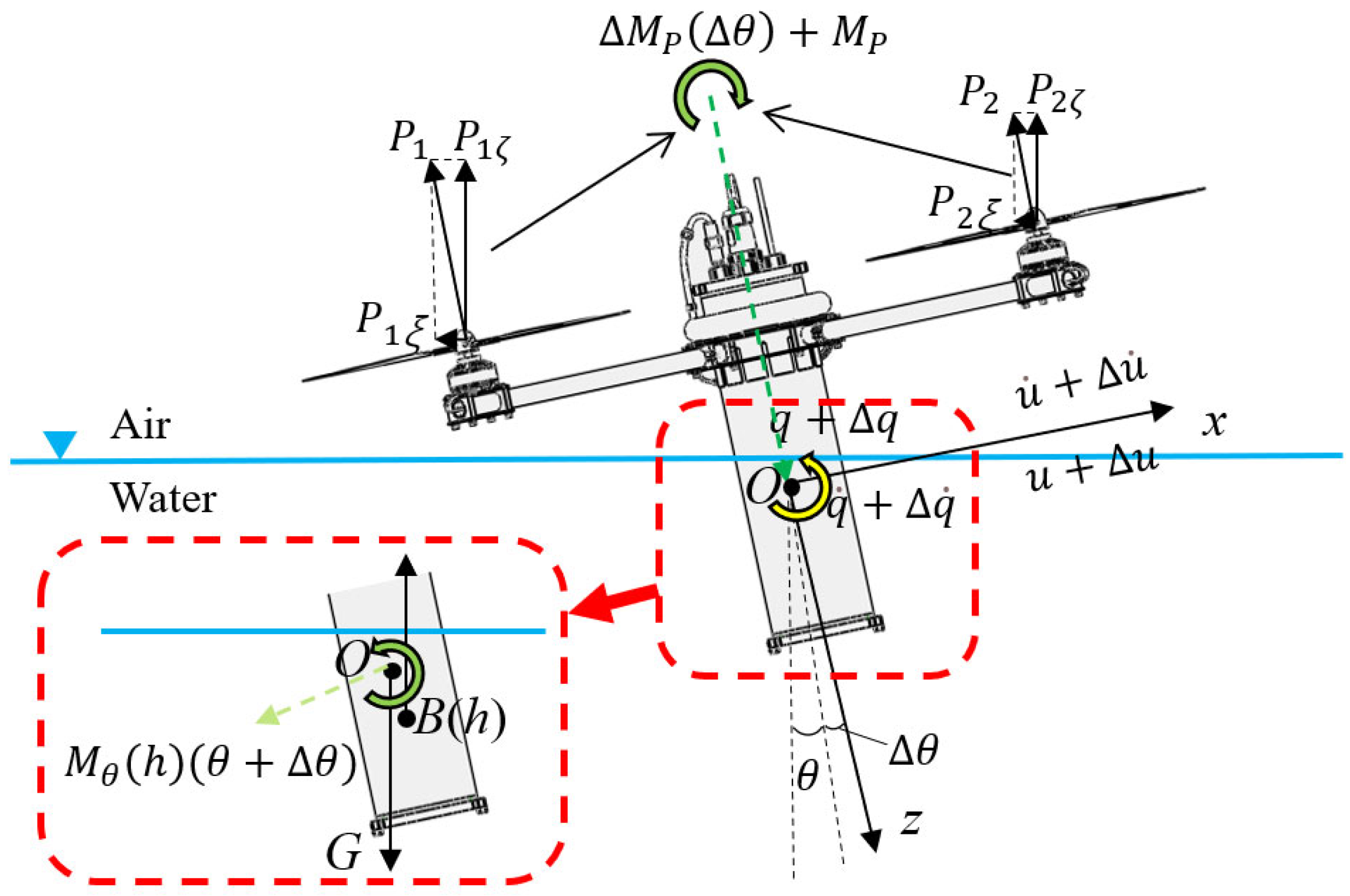
- (1)
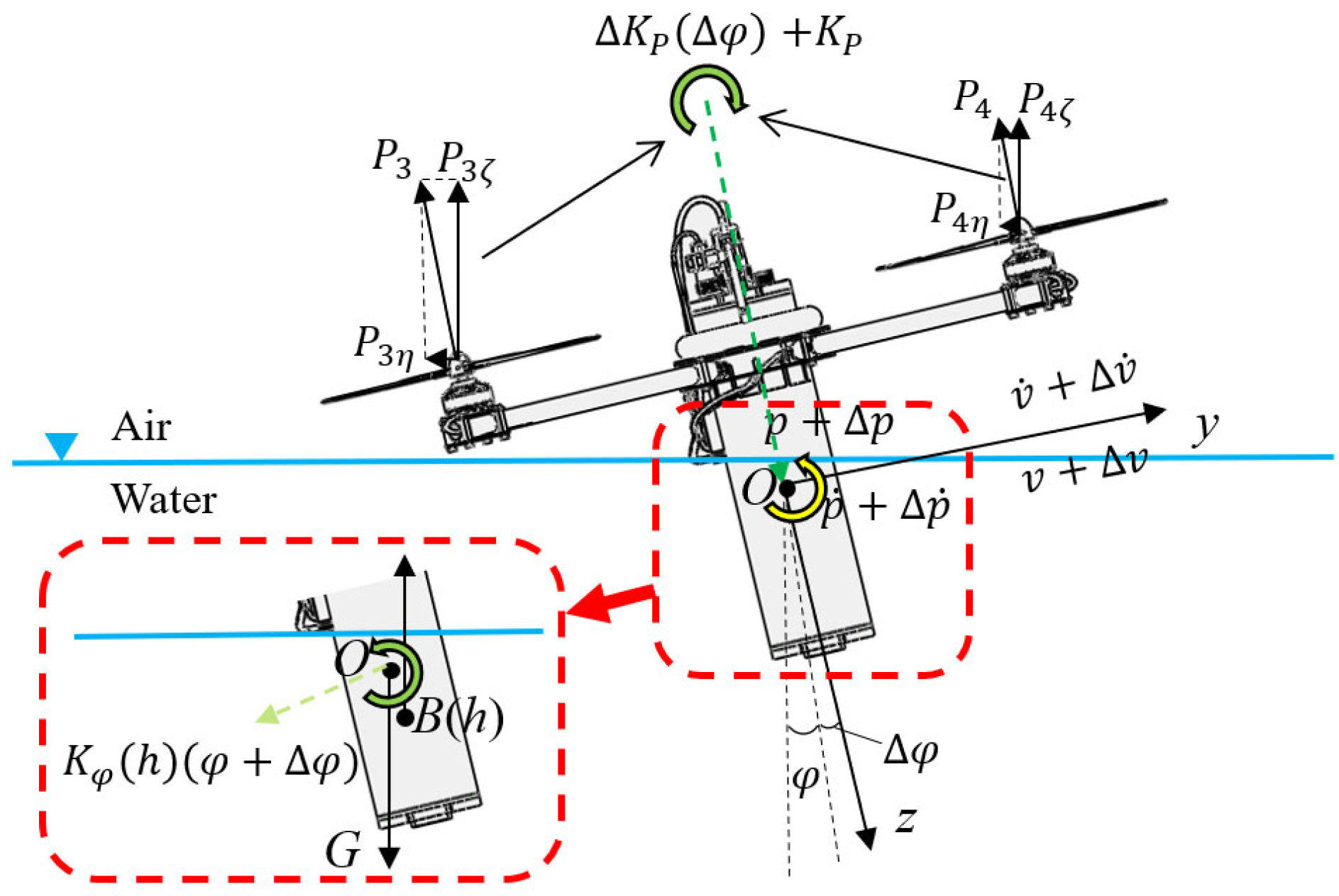
- In the process of air–water trans–media motion, a negative restoring moment occurs to accelerate the capsizing of the HAUV. In other words, the HAUV is not statically stable according to the classical theory. However, the classical static stability analysis does not include the thrust provided by the thrusters, which is necessary for the HAUV during the air–water trans–media process. Because there is no thrust, there is no air–water trans-media process. In this paper, the thrust and torque provided by the thrusters are taken into account in the static stability analysis.
- (2)
- The vehicle is subjected to disturbances of wind, wave and current in the air–water trans-media process in reality. These disturbances are superimposed with the overturning moment mentioned above, and consequently a severer negative force is experienced by the vehicle. In this paper, these disturbances are simplified. The influence of these disturbances on HAUV is considered roughly through the change of motion state, such as .
- (3)
- The hydrodynamic coefficients of Nezha are time–varying when the vehicle travels through the water’s surface, which greatly influences the dynamic stability of the vehicle during the air–water trans–media process.
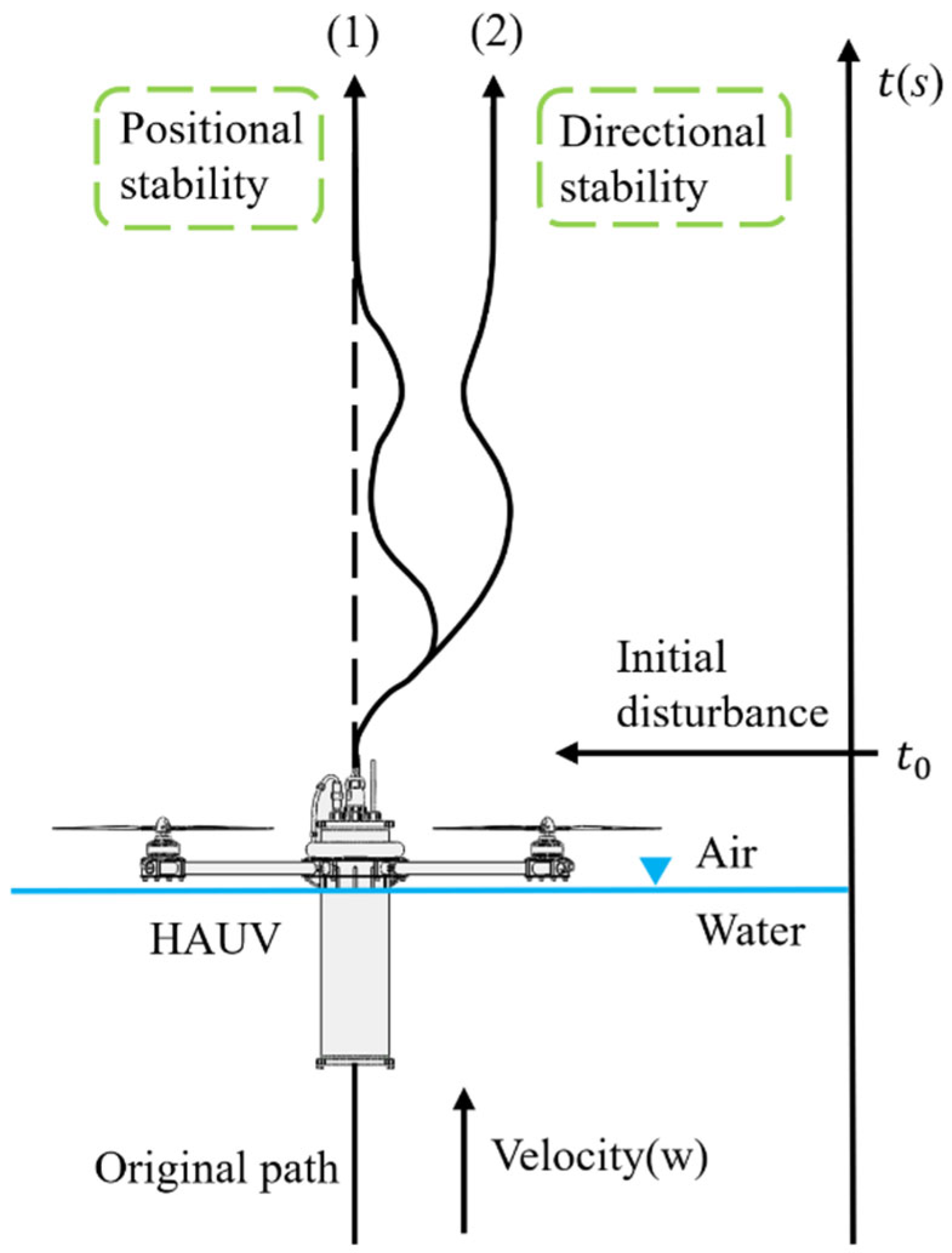
2.3. Definition of Kinematic Stability
- (1)
- Positional stability: After the initial disturbance, if .
- (2)
- Directional stability: After the initial disturbance, if .
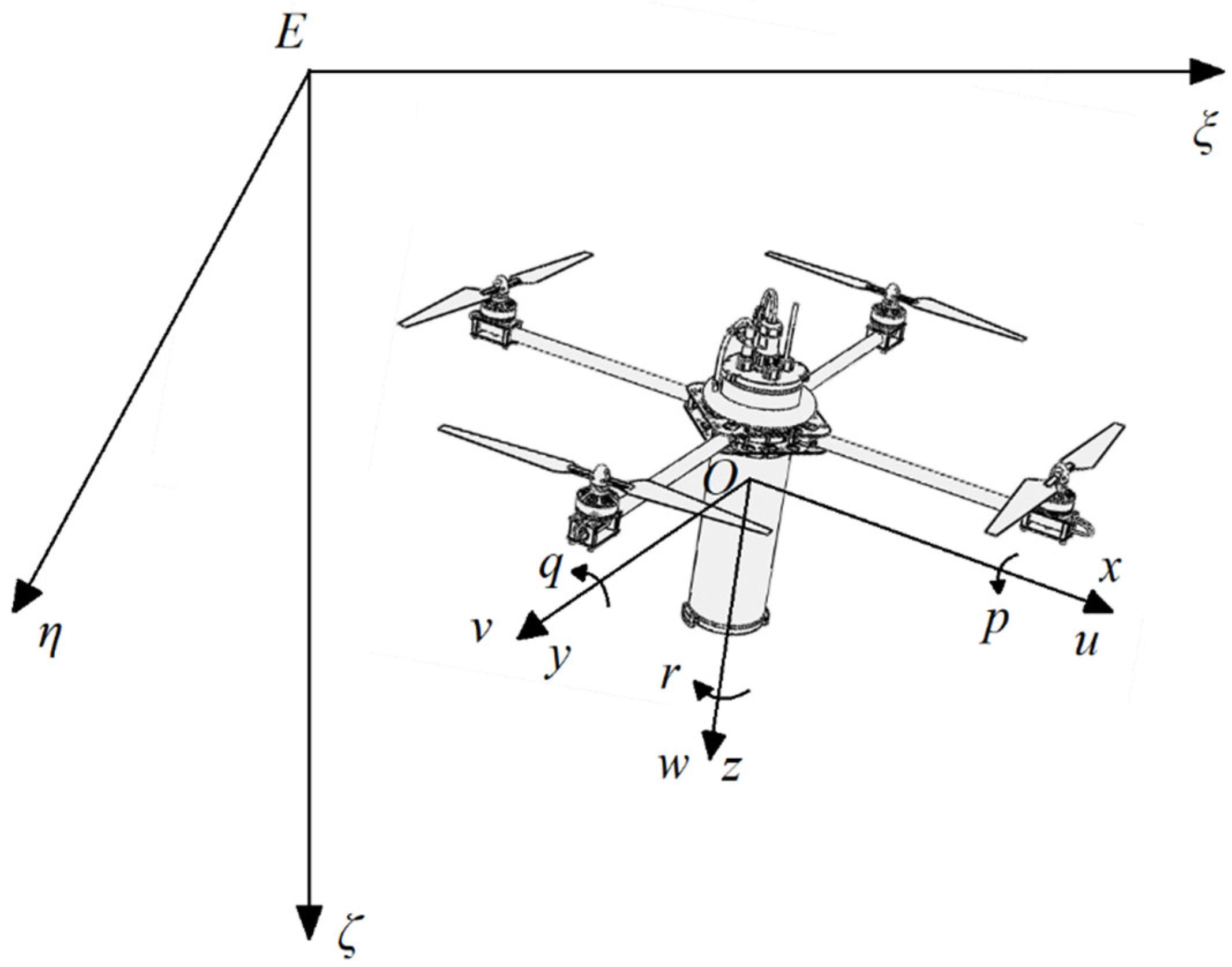
3. Model and Simplification
- (1)
- Since the rate of change of acceleration in the trans–media process of Nezha is very low, we believe that the motion of Nezha in the trans–media process satisfies the “slow–motion” hypothesis.
- (2)
4. Trans–Media Kinematic Stability Criterion
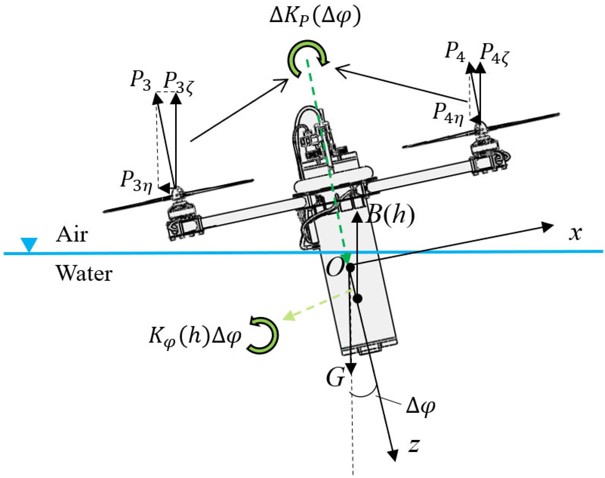
4.1. Trans–Media Kinematic Stability Criterion in ξEζ Plane
4.1.1. Static Stability
4.1.2. Dynamical Stability
4.2. Trans–Media Kinematic Stability Criterion in the Plane
4.2.1. Static Stability
4.2.2. Dynamical Stability
5. Trans–Media Kinematic Stability Analysis
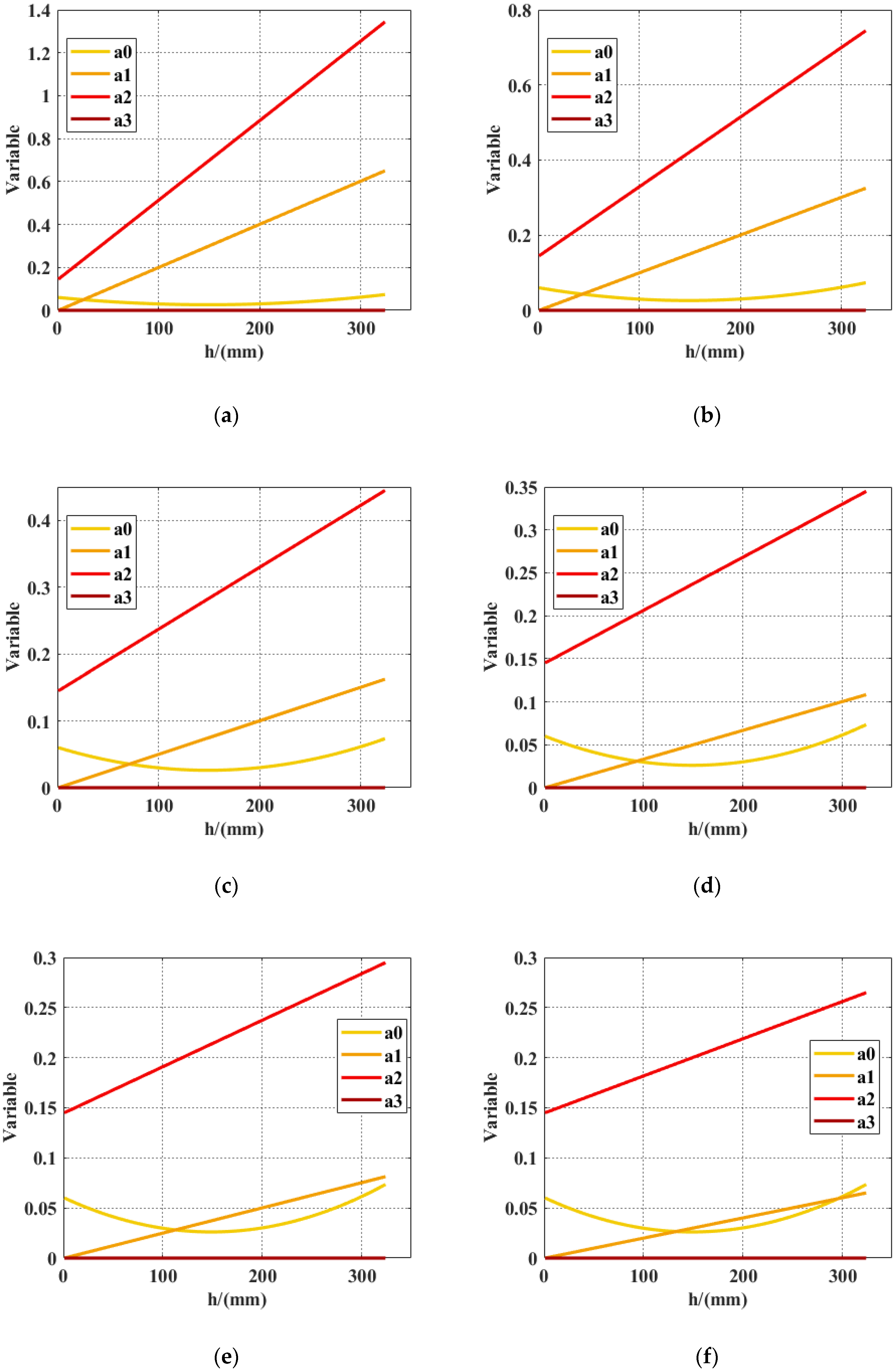
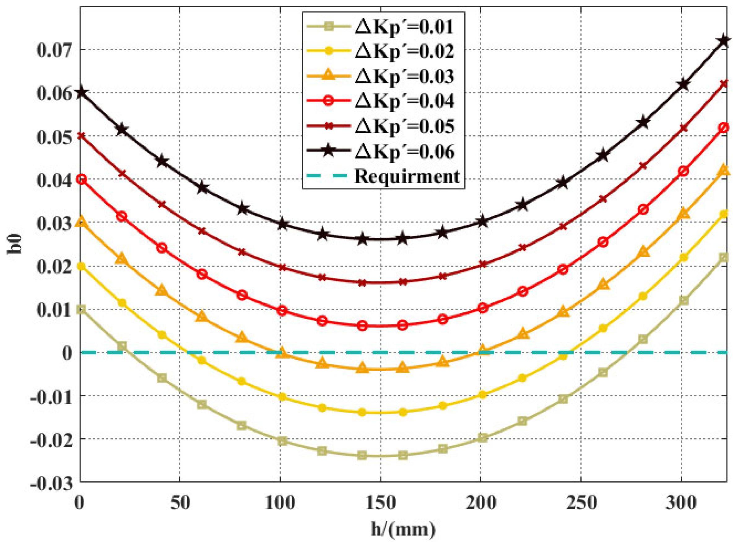
5.1. Trans–Media Kinematic Stability Analysis in the Plane
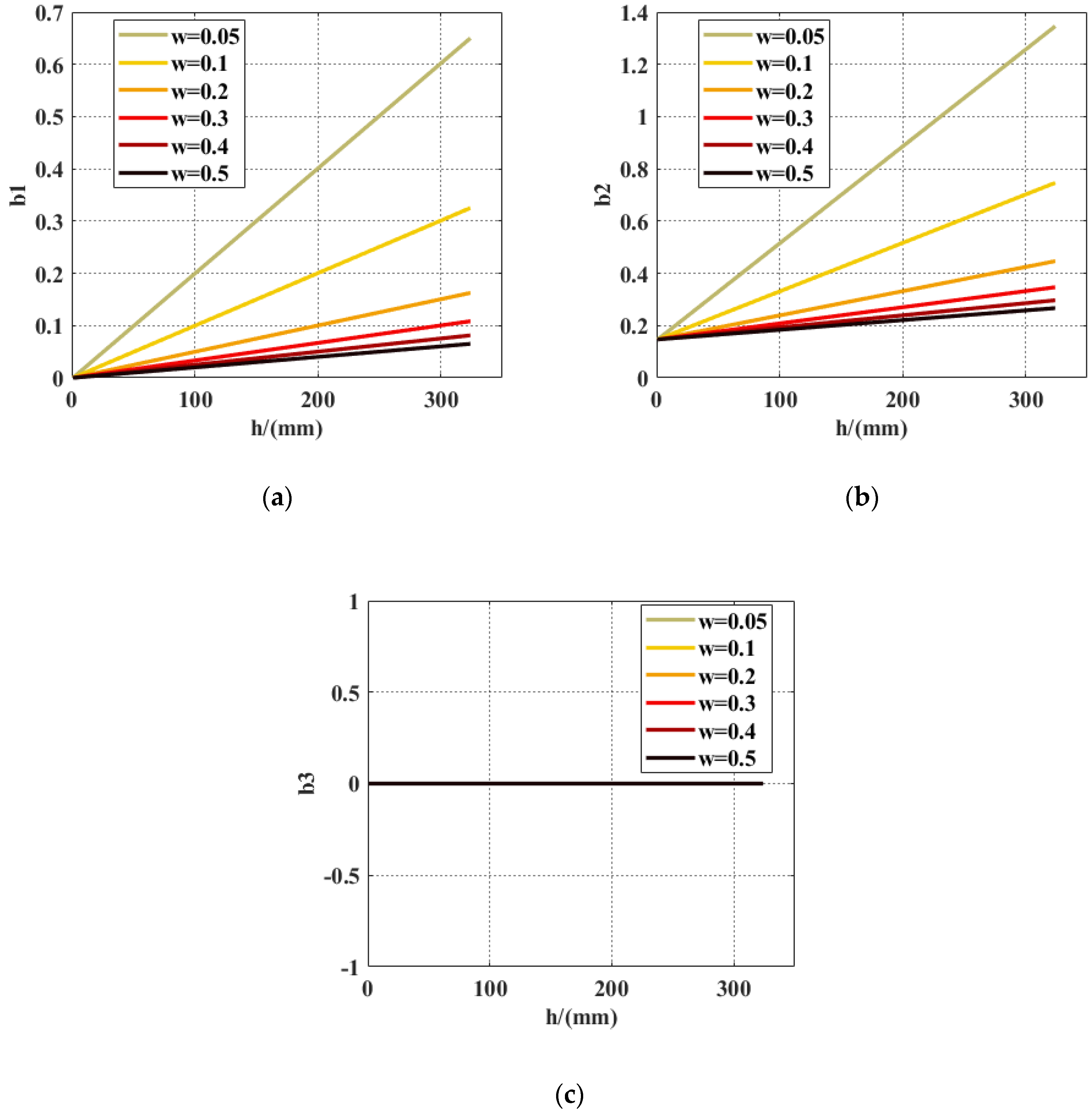
- (1)
- 0 < h ≤ 0.148 m: The impact of the restoring moment is negative, and the negative effect gradually increases. In this process, the buoyancy increases, and the restoring arm decreases gradually. The change of buoyancy plays a major role.
- (2)
- 0.148 m < h ≤ 0.296 m: The effect of the restoring moment is negative, but the negative effect gradually decreases. In this process, buoyancy increases, and the restoring arm decreases. The change of the restoring arm plays a major role.
- (3)
- 0.296 m < h ≤ 0.323 m: The effect of the restoring moment is positive, and the positive effect gradually increases. In this process, the buoyancy and the restoring arm increase.
5.2. Trans–Media Kinematic Stability Analysis in Plane
6. Conclusions
Author Contributions
Funding
Informed Consent Statement
Conflicts of Interest
Appendix A
References
- Maia, M.M.; Mercado, D.A.; Diez, F.J. Design and implementation of multirotor aerial–underwater vehicles with experimental results. In Proceedings of the 2017 IEEE/RSJ International Conference on Intelligent Robots and Systems (IROS), Vancouver, BC, Canada, 24–28 September 2017. [Google Scholar]
- Ravell, D.A.M.; Maia, M.M.; Diez, F.J. Modeling and control of unmanned aerial/underwater vehicles using hybrid control. Control. Eng. Pract. 2018, 76, 112–122. [Google Scholar] [CrossRef]
- Moore, J.; Fein, A.; Setzler, W. Design and Analysis of a Fixed–Wing Unmanned Aerial–Aquatic Vehicle. In Proceedings of the 2018 IEEE International Conference on Robotics and Automation (ICRA), Brisbane, Australia, 21–25 May 2018. [Google Scholar]
- Alzu’bi, H.; Mansour, I.; Rawashdeh, O. Loon Copter: Implementation of a hybrid unmanned aquatic–aerial quadcopter with active buoyancy control. J. Field Robot. 2018, 35, 764–778. [Google Scholar] [CrossRef]
- Stewart, W.; Weisler, W.; Anderson, M.; Bryant, M.; Peters, K. Dynamic Modeling of Passively Draining Structures for Aerial–Aquatic Unmanned Vehicles. IEEE J. Ocean. Eng. 2020, 45, 840–850. [Google Scholar] [CrossRef]
- Weisler, W.; Stewart, W.; Anderson, M.B.; Peters, K.J.; Gopalarathnam, A.; Bryant, M. Testing and Characterization of a Fixed Wing Cross–Domain Unmanned Vehicle Operating in Aerial and Underwater Environments. IEEE J. Ocean. Eng. 2018, 43, 969–982. [Google Scholar] [CrossRef]
- Lu, D.; Xiong, C.; Zeng, Z.; Lian, L. A Multimodal Aerial Underwater Vehicle with Extended Endurance and Capabilities. In Proceedings of the 2019 International Conference on Robotics and Automation (ICRA), Montreal, QC, Canada, 20–24 May 2019. [Google Scholar]
- Zongcheng, M.; Danqiang, C.; Guoshuai, L.; Junjie, Z. Constrained adaptive backstepping take-off control for a morphing hybrid aerial underwater vehicle. Ocean Eng. 2020, 213, 107666. [Google Scholar] [CrossRef]
- Abkowitz, M.A. Lectures on Ship Hydrodynamics–Steering and Manoeuvrability; Report Hy–5; Hydro–and Aerodynamic Laboratory: Lyngby, Denmark, 1964. [Google Scholar]
- Gertler, M.; Hagen, G.R. Standard Equations of Motion for Submarine Simulation; David w Taylor Naval Ship Research and Development Center: Bethesda, MD, USA, 1967. [Google Scholar]
- Fossen, T.I. Guidance and Control of Ocean Vehicles. Doctors Thesis, University of Trondheim, Trondheim, Norway, 1994. [Google Scholar]
- Leonard, N.E. Stability of a bottom–heavy underwater vehicle. Automatica 1997, 33, 331–346. [Google Scholar] [CrossRef] [Green Version]
- Palmer, A.R. Analysis of the Propulsion and Manoeuvring Characteristics of Survey–Style AUVs and the Development of a Multi–Purpose AUV; University of Southampton: Southampton, UK, 2009. [Google Scholar]
- Chen, C.-W.; Jiang, Y.; Huang, H.-C.; Ji, D.-X.; Sun, G.-Q.; Yu, Z.; Chen, Y. Computational fluid dynamics study of the motion stability of an autonomous underwater helicopter. Ocean Eng. 2017, 143, 227–239. [Google Scholar] [CrossRef]
- Ayyangar, V.; Krishnankutty, P.; Korulla, M.; Panigrahi, P. Stability analysis of a positively buoyant underwater vehicle in vertical plane for a level flight at varying buoyancy, BG and speeds. Ocean Eng. 2018, 148, 331–348. [Google Scholar] [CrossRef]
- Meng, L.; Lin, Y.; Gu, H.; Bai, G.; Su, T.-C. Study on dynamic characteristics analysis of underwater dynamic docking device. Ocean Eng. 2019, 180, 1–9. [Google Scholar] [CrossRef]
- Zhang, Q.; Hu, J.-H.; Feng, J.-F.; Xu, B.-W.; Liu, A. Motion law and density influence of a submersible aerial vehicle in the water–exit process. Fluid Dyn. Res. 2018, 50, 065516. [Google Scholar] [CrossRef]
- Ma, Z.; Feng, J.; Yang, J. Research on vertical air–water trans–media control of Hybrid Unmanned Aerial Underwater Vehicles based on adaptive sliding mode dynamical surface control. Int. J. Adv. Robot. Syst. 2018, 15, 1729881418770531. [Google Scholar] [CrossRef] [Green Version]
- Ma, Z.; Hu, J.; Feng, J.; Liu, A.; Chen, G. A longitudinal air–water trans–media dynamic model for slender vehicles under low–speed condition. Nonlinear Dyn. 2019, 99, 1195–1210. [Google Scholar] [CrossRef]


| Parameter | Value | Unit | Description |
|---|---|---|---|
| 3.473 | kg | Mass of the vehicle | |
| () | (0, 0, 0.148) | m | Centre–of–gravity position |
| 0.147 | kg∙m2 | Mass moment of inertia | |
| 0.145 | kg∙m2 | Mass moment of inertia | |
| 0.120 | m | Diameter of the cylinder | |
| 0.323 | m | Length of the cylinder | |
| 0.016 | m | Diameter of the arm | |
| 0.300 | m | Length of the arm |
| Variable | Definition | Unit | Variable | Definition | Unit |
|---|---|---|---|---|---|
| –coefficient representing effect due to | –coefficient representing effect due to | ||||
| –coefficient representing effect due to | –coefficient representing effect due to | ||||
| –coefficient representing effect due to | –coefficient representing effect due to | ||||
| –coefficient representing effect due to | –coefficient representing effect due to | ||||
| –coefficient representing effect due to | –coefficient representing effect due to | ||||
| –coefficient representing effect due to | –coefficient representing effect due to | ||||
| –coefficient representing effect due to | –coefficient representing effect due to | ||||
| –coefficient representing effect due to | –coefficient representing effect due to | ||||
| –coefficient representing effect due to | –coefficient representing effect due to | ||||
| –coefficient representing effect due to | –coefficient representing effect due to | ||||
| –coefficient representing effect due to | –coefficient representing effect due to | ||||
| Moment of the propeller in direction | Force of the propeller in direction | ||||
| Moment of the propeller in direction | Force of the propeller in direction | ||||
| Force of the propeller in direction | – | – | – |
Publisher’s Note: MDPI stays neutral with regard to jurisdictional claims in published maps and institutional affiliations. |
© 2022 by the authors. Licensee MDPI, Basel, Switzerland. This article is an open access article distributed under the terms and conditions of the Creative Commons Attribution (CC BY) license (https://creativecommons.org/licenses/by/4.0/).
Share and Cite
Wei, T.; Lu, D.; Zeng, Z.; Lian, L. Trans-Media Kinematic Stability Analysis for Hybrid Unmanned Aerial Underwater Vehicle. J. Mar. Sci. Eng. 2022, 10, 275. https://doi.org/10.3390/jmse10020275
Wei T, Lu D, Zeng Z, Lian L. Trans-Media Kinematic Stability Analysis for Hybrid Unmanned Aerial Underwater Vehicle. Journal of Marine Science and Engineering. 2022; 10(2):275. https://doi.org/10.3390/jmse10020275
Chicago/Turabian StyleWei, Tongjin, Di Lu, Zheng Zeng, and Lian Lian. 2022. "Trans-Media Kinematic Stability Analysis for Hybrid Unmanned Aerial Underwater Vehicle" Journal of Marine Science and Engineering 10, no. 2: 275. https://doi.org/10.3390/jmse10020275
APA StyleWei, T., Lu, D., Zeng, Z., & Lian, L. (2022). Trans-Media Kinematic Stability Analysis for Hybrid Unmanned Aerial Underwater Vehicle. Journal of Marine Science and Engineering, 10(2), 275. https://doi.org/10.3390/jmse10020275