An Open-Source Processing Pipeline for Quad-Dominant Mesh Generation for Class-Compliant Ship Structural Analysis

Abstract

We present an algorithm for the fully automatic generation of a class-compliant mesh for ship structural analysis. Our algorithm is implemented as an end-to-end solution. It starts from a description of a geometry and produces a class conforming surface mesh as a result. The algorithm consists of two parts, the automatic geometry refinement and the preconditioned Delaunay frontal quad dominant mesh generator. A geometry is described by a dictionary of elements and it contains points, rods, plates, and openings. A dictionary can contain modeling errors such as unintended overlaps or an unintended loss of connectivity between elements. The main contribution of the paper is the automatic geometry refinement algorithm and the virtual stiffener procedure designed to control the local mesh orientation of a marching front meshing algorithm. The geometry refinement algorithm guarantees that the output dictionary will be such that intersections of the boundary edges of plates are guaranteed to be nodes of any mesh generated by tessellating such geometry. The algorithm is implemented in Python, using the open-source Gmsh system together with the Open CASCADE kernel which is used to implement the automatic geometry refinement. We present several benchmark models from an engineering practice to illustrate our claims as well as to benchmark the efficiency of the various stages of the processing pipeline.

1. Introduction

In this paper, we study algorithmic solutions for the fully automatic mesh generation in ship structural analysis. The classification societies’ rules [1,2], for the finite element analysis include restrictions on the type of elements allowed, as well as rules for generating and assessing the quality of the wire-frame model (mesh). A general optimization instruction is that a mesh should mostly consist of quadrilaterals whose shapes are close to a square. There is a general restriction on the mesh that there should be no hanging nodes (elements of a mesh should only intersect on a joint edge or a joint node or the intersection is empty) and that the internal angles of the elements should be between 45° and 135°. In order to be definite, we have summarized the requirements on the mesh in Appendix A (coarse mesh description is in Appendix A.1, and the specifications for the fine mesh regions are in Appendix A.2). The contribution of this paper is the fully automatic algorithm which contains both the automatic geometric refinement procedure, which removes the connectivity and overlap errors in the geometry, and an automatic quad oriented mesh generator, which produces a mesh optimized according to the rules of the classification societies, see [1,2,3]. The algorithm is intended for the automatic coarse mesh generation for ship substructures in the early phases of the design process. Subsequently, the optimization objective is formulated according to the rules for generating a coarse mesh (Appendix A.1).

From an algorithmic perspective, these restrictions are to be interpreted as optimization instructions. This statement can better be understood when assessing the meshes presented as conforming to the classification societies’ rules in [1,2]. Meshes such as those presented on p. 31, p. 32, p. 37, and in particular p. 69 of [2] clearly contain few elements which violate the restrictions from Appendix A.1 and Appendix A.2 in the strictly formal sense. Subsequently, it only makes sense to implement the restrictions in the penalization sense. Note that the violation of the meshing restrictions is either due to the presence of a distorted triangle or quadrilateral (e.g., with an internal angle less than 45° or more than 135°) or by the presence of those with a bad aspect ratio. In the cited examples, such elements can also be seen in high stress regions. Subsequently, our approach to measure the quality of an automatically generated mesh, which will be described in detail below, is to use statistical quality measures. These quality measures are then to be used to define the stopping criterion for the mesh generation algorithm.

On the high level, there are three approaches to mesh generation in structural analysis of thin walled structures, [3]:

M1

Automatic/batch meshing. It is assumed that the geometry description has been corrected for connectivity errors before the algorithm is applied.

M2

Mapped or interactive meshing. In this approach, there is more human involvement than in the batch meshing but less than in fully manually generated mesh. It is also assumed that the geometry description has been corrected for connectivity errors before the processing pipeline is applied.

M3

Manual meshing where the meshing is intertwined with geometric modeling by the use of special graphical commands which correct the modeling errors by refining/idealizing the geometry based on a human decision.

These approaches have been implemented in the state of the art general modeling software such as Femap, Abaqus, Altair Hypermesh, or ANSYS Workbench. All of these general CAE tools offer automatic meshing options. However, these are designed for general meshing tasks and require time-consuming interactive sizing and mesh orientation control to implement the rules of classification societies. We provide an exemplary review of two of these general meshing solutions, where we were able to find explicit references in the literature. In the Hypermesh, the automatic meshing procedure is implemented as the HM-Authomesh algorithm, see [4]. On the other hand, Ansys Workbench has an automatic surface meshing procedures called quad dominant meshing for generating coarser meshes and uniform quad/tri method which generates a fine mesh, see [5]. According to [6], this procedures are in part based on the QMorph algorithm.

As described in [7], the quadrilateral dominant meshing procedure was controlled by the size field, which is a result of an action by a user. The quality of the meshes is described using the element quality indicator which is the ratio of the area to edge length (one indicates the perfect square) and the skewness criterion, an angle dependent metric measuring the distance of an element to a regular quadrilateral. These quality measures roughly correspond to the mesh size field and quadrilateral shape measure indicators from [8,9]. The protocol to use the uniform quad method starts by determining a small regular element size, and then this element size is uniformly used to resolve the whole model. This often results in a mesh far too fine (see [7], Section 4) for the initial phases of the design process or for the use in, e.g., the automatic sizing optimization procedures. This is the niche for which we are proposing our algorithmic solution. As a result of running the meshing algorithm, a statistics of the performance of the indicators is presented. We will use a similar approach to measure the adherence to the rules of classification societies.

On the other hand, specialized tools for ship structural analysis such as MAESTRO1 use interactive meshing solutions implemented in Rhinoceros2, NAPA Steel3, or Femap4 for the same purpose. They also rely on the interactive input by an expert. In all of these approaches, it is assumed that the connectivity errors have been removed by specialized tools which were applied prior to running an automatic or an interactive mesher [3]. Furthermore, tools for interactive defeaturing (idealizing) of the geometry and/or for removing overlaps between elements might also have been used in order to defeature parts of the geometry which incur the need for very fine meshes or cause the introduction of low quality elements.

To gain some intuition of what is expected, let us quote some instructions from a manual. According to [4], a mesh which is fully automatically generated (i.e., not by using incremental meshing) on a hand refined geometry and has “approximately” between 80% and 90% elements of “good quality” is still considered as an acceptable output from the automatic mesher5. It is assumed that further mesh refinement will then be performed by hand judiciously using mesh join and refine operations. We will use these particular thresholds for benchmarking, as we were not able to find other explicit statements to this effect in other sources which were available to us.

As the notion of the regular element has not been formally defined, and in particular not in the context of the meshing rules as posed by the classification societies ([2], Sections 1.7 and 3–2.2.4), we will provide our own quality measures and use them to compare various versions of the algorithm. To this end, we define a regular element as a quadrilateral or triangle with internal angles between 80° and 100° and aspect ratio less than 1:3 for quadrilaterals and 1:5 for triangles. We aim to have the relative ratio of these elements in a mesh higher than 80% and then drive it as high as possible by automatically controlling the cross-field (a heuristic function defined by the geometry which determines the local mesh orientation). A further statistical measure will be the ratio of conforming elements (those are elements having internal angles between 45°and 135° and aspect ratios better than 1:3 for quadrilaterals and 1:5 for triangles) in the list of all elements. We will call these elements cs-conforming and will aim to have this ratio higher than 95%. Finally, we will track the ratio of the triangles in the mesh and will aim to drive this ratio below 5%. This is our quantitative interpretation of the mesh quality guidelines posed by the classification societies, see Appendix A.

In general, a run of a meshing algorithm can be divided in two phases. The first phase is the geometry correction and it involves some geometry processing operations and/or idealizations. The second phase is the automatic surface mesh generation for the geometry described by the corrected description. In this paper, an input to the algorithm will be a geometry formally described as a dictionary of elements (points, rods, and plates), together with a list of openings in the specified plates. This dictionary of elements and the list of openings (which will be termed as holes in the rest of the paper) is the formal description of a geometry. The first step of the algorithm is to preprocess the problem by cleaning the geometry (removing overlaps and correcting the connectivity of hanging surfaces). The output will be a surface mesh of the refined geometry in the Gmsh format [8]. The output mesh will be generated so that it adheres, in a statistical sense, to the restrictions outlined in Appendix A.1. The algorithm will be aggressively optimized towards producing meshes with fewer nodes. Subsequently, we will not be generating a fine mesh surrounding a hole, as this would require a mapped mesh generation. Instead, the mesh transition will be as produced by the marching front algorithm. We argue, by the use of statistical indicators, that the use of the $L^{\infty }$ marching front Delaunay mesh generation will produce meshes of sufficient quality. The algorithm which we propose is implemented in Python and is released under GNU general public license, Version 3 (GPLv3) and can be accessed at 23 December 2021 https://github.com/PMF-ZNMZR/pyREMAKEmsh (accessed on 23 December 2021).

Let us now review the state of the art. We will briefly review the meshing algorithms reported in the academic journals. The paper [10] is the closest in spirit to the specifications of the task which we consider. It starts with a 3D CAD geometry model and aims to automatically obtain a mesh of FEs suitable for ship structural analysis. The paper describes an algorithm called the stiffener-based mesh generation. A problem with direct application of the QMorph algorithm on ship structures is that the resulting mesh is very often too fine (meaning that we unnecessarily end up with too many FEs), which is a consequence of regarding the stiffeners as line constraints in the mesh generation process. The main idea of the paper is, thus, to use stiffeners (i.e., stiffener lines) in the surface decomposition (subdivision) as edges of the newly created subsurfaces rather than line constraints during the mesh generation. This way, the number of the resulting FEs can be controlled much easier and can be adapted to the requirements of the ship structural analysis. The paper demonstrates the application of the algorithm on a partial and a full ship model of a tanker and a container ship and compares the obtained meshes with those that are generated manually. The resulting meshes seem to correspond to each other to a high degree. However, there are no quality measures defined explicitly, so the comparison is somewhat moot. In addition, although the resulting meshes seem to fulfill most of the classification societies’ criteria on the FEA, an explicit implementation of the criteria in the algorithm seems to be missing. Consequently, it is difficult to assess the resulting meshes with respect to the criteria (e.g., the fraction of triangular or irregular quadrilateral elements). An example of how to use a statistical criterion for assessing the mesh quality can be seen in ([7], Section 4).

The notion of the line constraint in a Delaunay mesh generator has been introduced in [11]. There the geometric elements have polygonal lines as boundaries. The polygonal lines can either be closed loops or they are called the line constraints. The paper [11] introduces also a more structured way to optically compare the resulting mesh with the results of Altair’s Hypermesh (automesh). A further interesting feature is the use of a shape regularity indicator for quadrilateral elements for which the authors a priori give thresholds for assessing the quality of the mesh using the statistics of the regularity indicator. In comparison, we use a larger class of quality measures which describe the rules of the classification societies more comprehensively. The papers [12,13,14] present recent accounts of the use of automatic meshing in ocean engineering for tasks such as structural optimization and hull shape optimization. In contrast, for this paper, we have a strict focus on the fully automatic structural analysis according to the rules of the classification societies. These restrictions are typically not tackled automatically by general automatic meshers.

A more recent contribution to the field is [15,16]. An approach that can efficiently generate FE meshes on complex surfaces defined by NURBS is proposed in [15]. A ship’s outer shell tends to be geometrically very complex in the fore and aft peaks. The proposed approach demonstrates how intersections between the outer shell surfaces and longitudinal and transverse structural elements can be obtained. These are subsequently used to generate a coarse mesh, which can be further refined. A measure of quality of the resulting meshes is given for quadrilateral elements in terms of their aspect ratio, warp, skew, taper, and the Jacobian. The workings of the proposed approach are demonstrated on a midship and a stern model of a container ship.

An algorithm that generates a FE mesh for longitudinal structural members starting from 2D drawings is demonstrated in [16]. The 2D drawings of transverse ship structures are analyzed and longitudinal members are extracted. Based on this, the FE mesh is created, skipping the phase of creating a 3D CAD model. The resulting mesh can be used in the global direct strength analysis of ships with pronounced longitudinal strength (e.g., tankers and bulk carriers).

It is important to note that the algorithms proposed in both [15,16] do not take into account the classification societies’ requirements. Consequently, they do not give any coherent set of quality measures that might be used in the assessment of the resulting meshes with respect to the requirements.

Meshes based on quadrilateral elements can either be generated directly by some sort of advancing front algorithm such as [17] or by a subdivision of a region in quadrilaterals using a regular grid-based methods (quadtree or octree algorithms) [18]. Alternatively, a quadrilateral mesh can be generated indirectly by a recombination of a triangular mesh. However, in this approach it is necessary that the original triangular mesh be generated so that a recombination yields a regular quadrilateral mesh. Quadrilateral elements in Gmsh are generated indirectly by the perfect matching algorithm based on the graph theoretic Blossom algorithm [19,20]. A default implementation starts from a standard Delaunay advancing front algorithm implemented in the $L^2$ metric.

An important extension and improvement to the Blossom algorithm based quadrilateral mesh generation is realized by adapting the triangular mesh generator so that the generated triangular mesh can be efficiently recombined into a regular quadrilateral mesh. It is achieved by modifying the advancing front Delaunay mesh generator with the change of norm from $L^2$ to the $L^{\infty }$ norm. In this way, the triangles which are generated by the Delaunay algorithm will tend to be closer to right angle triangles than in the $L^2$ case where the algorithm tends towards equilateral triangles, i.e., with angles closer to 60°, see [9]. 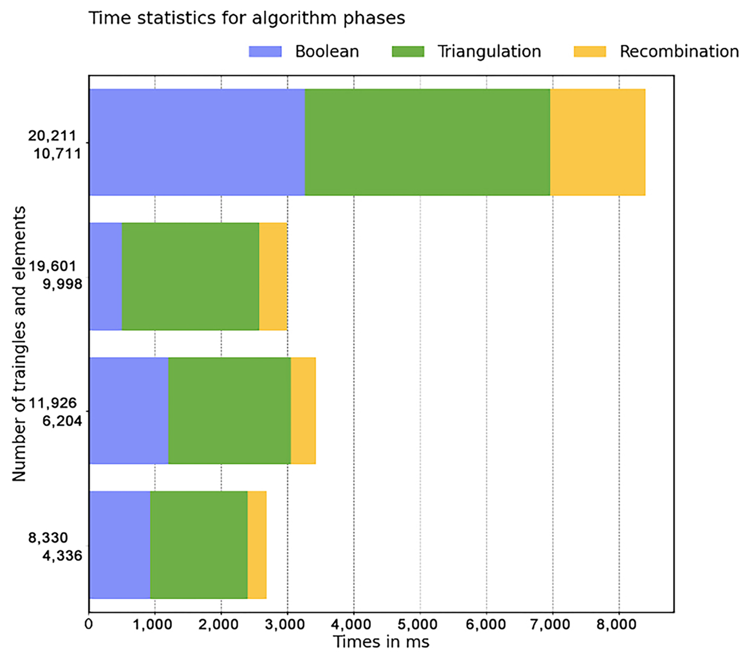The orientation of the mesh is dictated by the heuristic function called the cross-field, and it is this object that we will be utilizing through our modification, called the virtual stiffener algorithm, of the stiffener-based mesh generation from [10]. The overall timing, when discussing the efficiency of the algorithm, consists of two phases. The first phase is the triangulation phase, in which a triangular mesh, amenable to recombination into high quality quadrilaterals, is generated. The second phase is the recombination phase, in which the triangles are combined into quadrilaterals based on the minimal cost perfect matching algorithm. When reporting the performance of the algorithm, we will be reporting two numbers, the overall number of triangles and the final number of the elements (quadrilaterals and triangles) which were generated.

The use of triangle recombination in a quadrilateral mesh generator is not new in marine engineering. A notable example is the utilization of the qmorph algorithm in [5,21,22]. According to ([5], Section 5.3) this approach is available in several commercial meshers, including in Ansys, to automatically generate quad dominant meshes.

However, it was observed in [10] that such meshes can include lower quality quadrilaterals in a way which is not easy to control. The method proposed in [10], called Stiffener-Based Mesh Generation, achieved the control of the quality of quadrilateral meshes by subdividing the parts of the geometry adding extra stiffeners. A further improvement of the mesh was achieved by proactively modifying the geometry, e.g., by removing challenging parts of the geometry, in the procedure called idealization.

Our approach to the problem of generating high quality quadrilateral meshes for the structural analysis of marine structures is bases on the $L^{\infty }$ advancing front mesh generation algorithm from [9] in a combination with a minimally aggressive geometric preconditioning step. This preconditioning is primarily aimed to implement the restrictions posed by the rules of the classification societies restricting mesh generation, such as requiring precisely four elements per girder’s height, and restricting angles, in almost all cases, to the range between 45° and 135°. Let us point out that the classification societies, see ([2], Sections 3–2.2.4), depending on the particular scenario, require at least one two or three elements to resolve the girder height. We have implemented this restriction by requiring four elements per girder height. This is a compromise option which produces a compliant mesh which is, at the same time, fine enough to resolve the geometry of the girder when introducing openings. Furthermore, as a consequence of the utilization of the modeling software, there are frequent instances of overlapping plates which need to be idealized. To this end, we use Boolean geometric operations as implemented in a typical CAD geometric kernel. We use the Open CASCADE kernel6 which is intertwined with Gmsh and can be accessed through pygmsh Python module.

Our general approach to idealization was that the definition of the geometry should be respected as much as possible but that all overlaps should be removed automatically. We control the meshing algorithm by imposing restrictions on the cross-field (defining the orientation of an element) using virtual stiffeners. To be specific, the holes in the plates were localized by virtual stiffeners primarily for the purpose of enforcing the preference for quadrilaterals which have angles close to 90° and have sides parallel to boundaries of a plate in which they are punctured. In general, Blossom algorithm produces a quadrilateral mesh from any triangular mesh with even number of the triangles. Furthermore, the marching front quadrilateral Delaunay mesh generator produces triangles close to the right-angle triangle and so typically compensates inexactness in the definition of the surface, even in challenging situations, with at most a couple of acute angle triangles.

The makeup of the paper is as follows. We will first present materials and methods where we will describe the virtual stiffener algorithm for the control of the quadrilateral meshes generated by the algorithms from [9,19]. We will then present meshing results when applying these algorithms on several prototypical and realistic examples of ship substructures. In the discussion section, we will present statistical evaluation of the proposed algorithm. Finally, we will draw some conclusions about the use of open-source meshing software in naval architecture when comparing it to the interactively obtained meshes.

2. Materials and Methods

In this paper, we describe a geometry as a dictionary of elements, see Figure 1. The dictionaries which we consider consist of points, rods, surfaces, and openings. The points in the dictionary describe positions where the loads are applied or measurements are taken. Rods describe panel stiffeners or pillars. The set of surfaces consists of two types of entities: web surfaces (parallelograms with one dimension much smaller than the other) and regular surfaces (convex quadrilaterals defined by four co-planar nodes) [8,22]. Dictionaries which also include warped surfaces have been considered in a followup paper, see [23] for further details.

Let us note the following geometrical observation from ([9], Section 4.3). An equilateral triangle in the $L^{\infty }$ norm is isosceles in the $L^2$ norm. In fact, an equilateral triangle in the $L^{\infty }$ norm is half of the square. The marching front $L^{\infty }$ Delaunay algorithm generates a marching front of $L^{\infty }$ equilateral triangles, e.g., having angles close to the right angle, and pushes—by design—degenerate triangles to the boundary of the region to be tessellated. A subsequent application of the perfect matching algorithm from [19] yields a regular quadrilateral mesh with all of the degenerate triangles pushed to the boundary.

Modern quadrilateral meshing algorithms are designed around the notion of the cross field [24]. This is a heuristic function defined based on the geometry and it locally models the preferred orientation of the mesh. For a quadrilateral mesh generating algorithm, this is taken to be parallel to the boundaries of the domain. To compute the desired orientation of the mesh in a given node, the frontal meshing algorithms propagate this cross-field information from the boundaries and insert a point in the mesh so as to form an equilateral triangle. In the quad oriented algorithm, one uses the Delaunay approach in the $L^{\infty }$ norm, and so the equilateral triangle is actually isosceles with an angle close to a right-angle. These triangles can then be optimally matched into quadrilaterals using the graph theoretic approach which minimizes the measure of the departure of a quad (a pair of triangles) from regularity. Furthermore, the unmatched triangle will be pushed by the marching front to the boundary. In what follows, we will describe the basic properties of the algorithm and our method of imposing further line restrictions on the mesh by the addition of the virtual stiffeners to the model.

Let us define the quadrilateral mesh quality measures. For a quadrilateral q with internal angles ${\alpha }_i\left(q\right)$, $i=1,\cdots ,4$, we define the quadrilateral shape measure

$$\eta \left(q\right)=max\left[1-\frac{2}{\pi }\underset{i}{max}\left[|\frac{\pi }{2}-{\alpha }_i\left(q\right)|\right],0\right].$$

This quality measure is equal to one for the perfect rectangle and it is zero in the presence of angles which are less than zero or greater than the straight angle (a nonconvex quadrangle).

Let $G(V,E,c)$ be an undirected weighted graph. Here, V is a set of $n_V$ vertices, E is a set of $n_E$ undirected edges, and $c\left(E\right)={\displaystyle \sum _{e_j\in E}}c\left(e_{ij}\right)$ is an edge-based cost function. A matching is a subset $E^{\prime }$ of the set of edges such that a node V has, at most, one incident edge in $E^{\prime }$. A matching is called perfect if each node of V has exactly one incident edge in $E^{\prime }$. As a consequence, a perfect matching has exactly $n_{E^{\prime }}=n_V/2$ and can be only found in graphs with an even number of vertices. A matching is optimal if $c\left(E^{\prime }\right)$ is minimal among all possible perfect matchings.

In the case of triangle recombination, the graph $G(V,E,c)$ is defined by taking V to be the set of triangles and E to include those triangle pairs having a common edge. The matching is perfect if all triangles have been matched in quadrilaterals and it is optimal if

$$c\left(E^{\prime }\right)=\sum _{(e_1,e_2)\in E^{\prime }}(1-\eta \left(q_{12}\right))$$

is minimal over all subsets $E^{\prime }$. Here, $q_{12}$ is the quadrilateral obtained by merging a triangle pair $(e_1,e_2)$ from $E^{\prime }$. There are two options to apply the recombination algorithm in Gmsh. One is the full Blossom recombination algorithm which matches at least 99% of elements and the other simple Blossom recombination algorithm which stops when the introduction of further quad elements by matching triangles would decrease the quality of quadrilaterals as measured by $\eta$ [19,25].

To assess the quality of the generated mesh from the perspective of the rules of the clasification societies for the coarse mesh generation, see Appendix A.1, we will use the following statistical measures.

We define $\overline{\eta }$ as the average $\eta \left(q\right)$ taken over all quadrilaterals q in the mesh. We further measure the percentage of the triangles in the mesh $\tau$. By $\xi$, we denote the percentage of regular quadrilaterals (those with internal angles between 80° and 100°) in the mesh and use $\lambda$ to denote the percentage of the cs-confirming elements in the mesh. We point a reader to [7] to see a similar definition of the statistical performance measures for meshers in ship structural analysis.

2.1. Automatic Geometry Refinement Using Boolean Operations

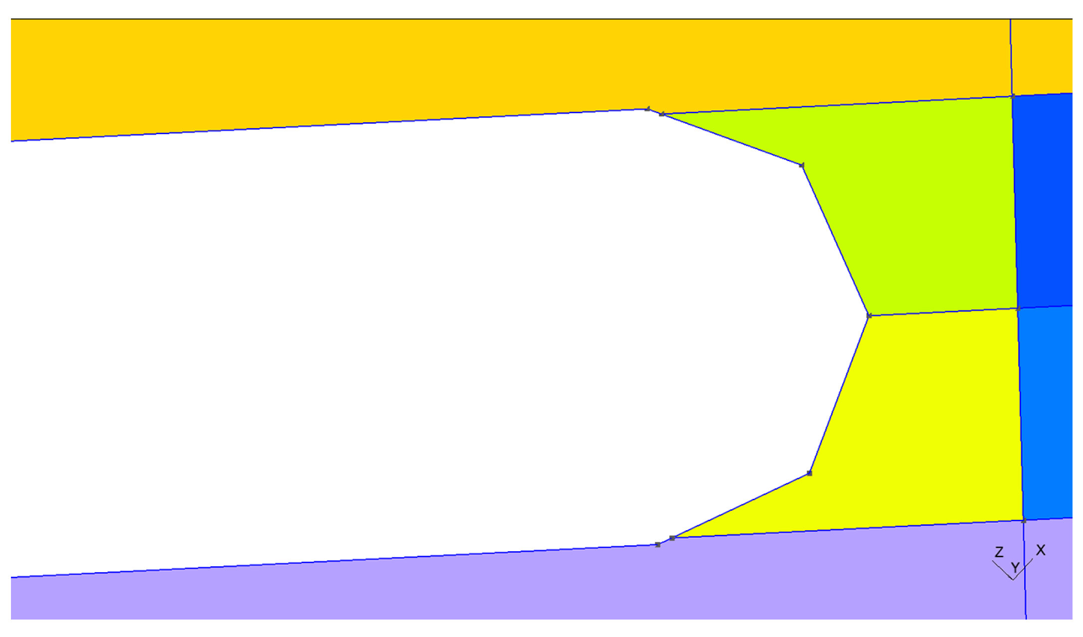
We will now briefly describe the effect of the Boolean operation on the geometry by considering two case studies. First, the unintended overlap of the two girders on Figure 2 and the effect of introducing a hole on the girder in Figure 3. The algorithm is restricted by the requirement that there are precisely four elements resolving the height of the girder. Subsequently, a Boolean operation resolving the overlap of a hole and a girder introduces a restriction incurring the use of possibly low-quality elements. We have tested our preconditioning algorithm on geometries requiring “coarse” meshes of up to hundred thousand elements with similar performance metrics. We note that in general the number of degenerate elements is minimized by an interactive approach which utilizes mesh mapping.

2.2. Automatic Mesh Generation Based on Virtual Stiffeners—Controlling the Local Mesh Orientation

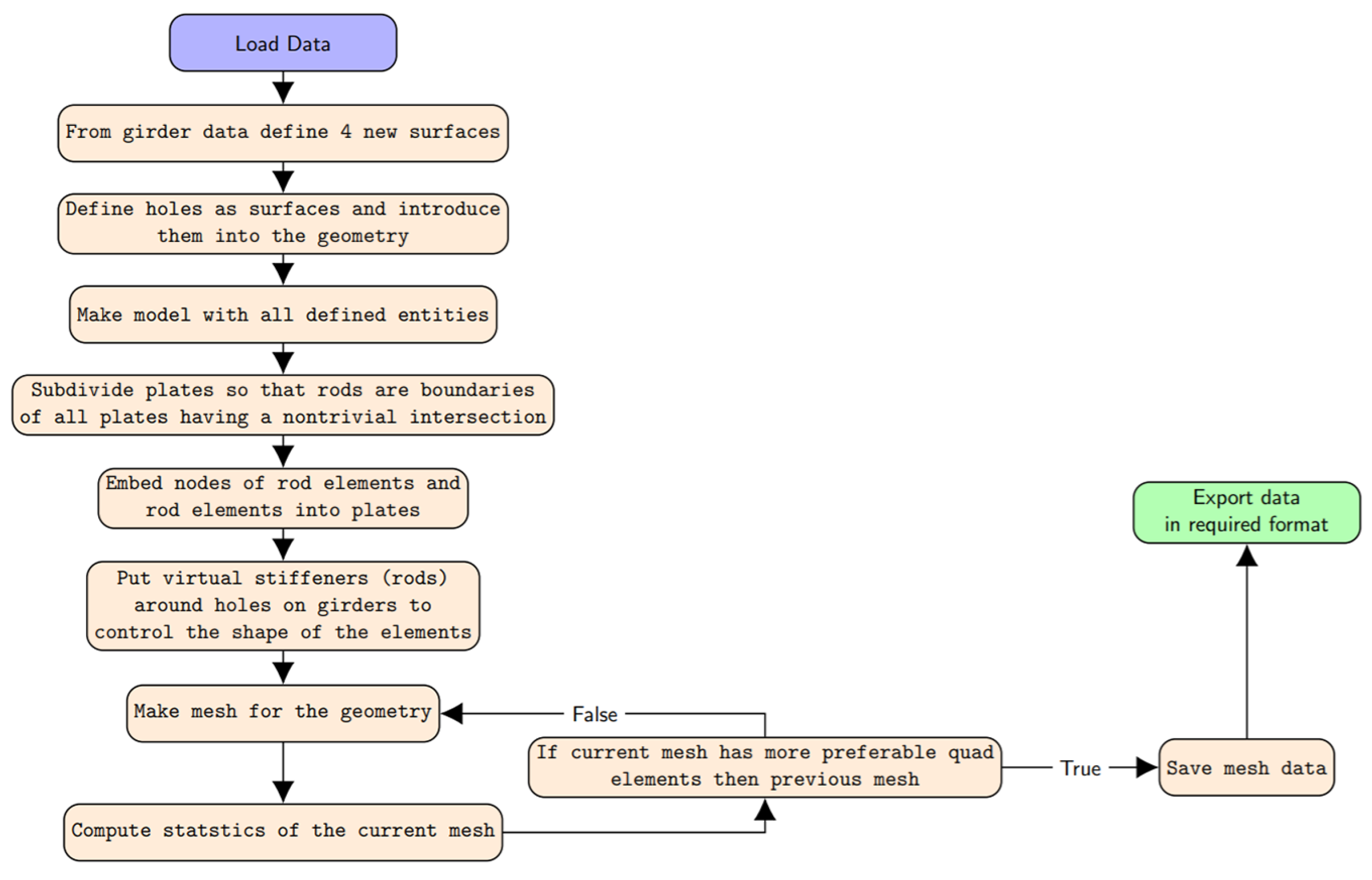
We will summarize the algorithm we implemented in the following flow chart (see Figure 4). On a high level, the algorithm consists of three parts. First, we preprocess the geometry to remove the overlapping surfaces. We further subdivide the surfaces along the stiffeners and ensure that all of the nodes on the stiffeners are nodes in the mesh. This step is implemented using the pygmsh library to access the highly optimized Boolean operations of the Open CASCADE geometric kernel. Second, we introduce virtual stiffeners to enforce the cross-field control on the quadrilateral elements. The virtual stiffeners are not bona fide one dimensional elements. They are not returned in the dictionary of one-dimensional elements and are only introduced to control the properties of the mesh around the holes in the structure and force the splitting of a surface in two surfaces with the desired cross field.

The newly generated surfaces inherit all of the properties of the parent surface. As the last step, we carry out a sequence of boundary-controlled refinements with the aim of determining the mesh with the lowermost number of nodes, in the sequence of refinements, with the highest percentage of regular quadrilaterals. For this part of the algorithm, we have used the Python interface to the Gmsh library of meshing routines. This allowed us to implement our algorithm based on the well tested and performance optimized routines—the Blossom perfect matching algorithm and the marching front Delaunay mesh generator. The implementation is described in Figure 4.

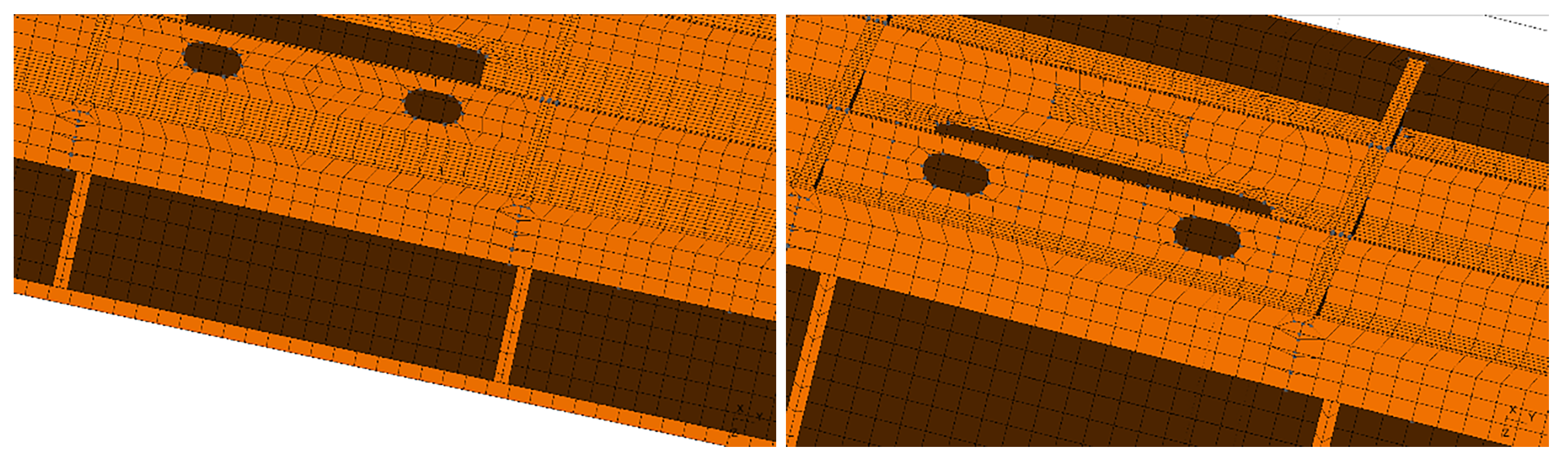
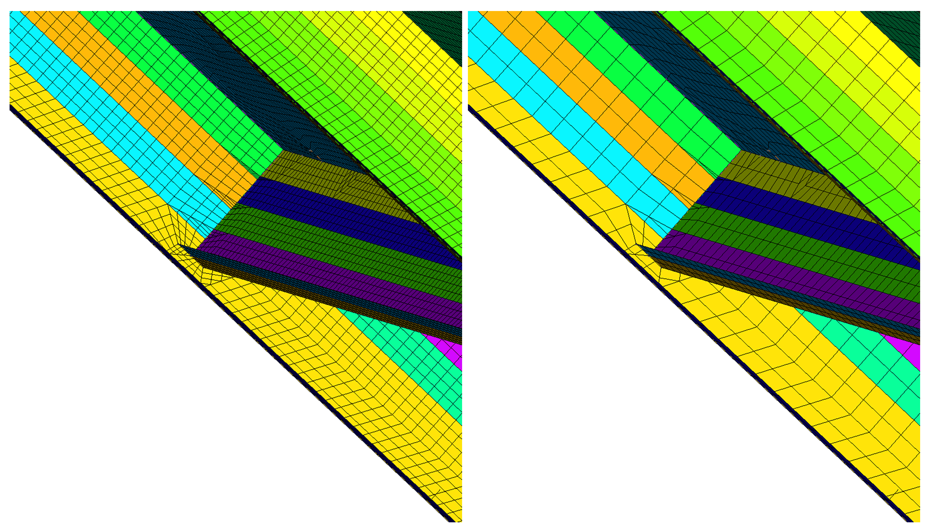
2.3. Controlling the Sizing Field of Web Surfaces

From the examples of ship structures presented thus far, we see that the main challenge for the mesher to produce the mesh conforming to the classification society’s rules is in handling the geometry of the web surfaces. Most of the degenerate elements are generated on the web surfaces as the consequence of the need to resolve the curved boundaries of the openings and to resolve the contacts of the girders of differing sizes. The rules of the classification societies stipulate that a web surface should be meshed with at least three elements per length of the shorter size (see [2], Sections 3–2.2.4).

Our stated optimization goal is to produce coarse meshes which are able to resolve the geometry features encountered when meshing ship substructures. We have opted to modify the requirement that a web surface should be meshed by at least three elements per length of the shorter side, while limiting the growth of the mesh size. We have opted adaptively generate four elements per shorter length of the web surface. The adaptivity first ensures that all of the openings are located in the two inner strips of elements. Then, we further control the size field in the Gmsh by running the Algorithm 1 on the collection of all web surfaces.

Algorithm 1: Mesh element size algorithm

$\mathrm{factor}=\left[\right]$ for S in web surfaces do       Divide S in 4 new surfaces along the shorter side       Calculate the size s of the shorter side of S       Append s to the array factor. end for Set $\overline{\mathrm{factor}}=\mathrm{average}\left(\mathrm{factor}\right)$ Set $\overline{\mathrm{factor}}$ as the minimal mesh size factor in Gmsh Set maximal mesh size factor in Gmsh as $1.5\ast \left(\overline{\mathrm{factor}}\right)$

3. Results

We will utilize two case studies for comparing the algorithms which we discussed in this note. The challenge in all of the models is to incorporate the line constraints in the mesh (e.g., stiffeners or girders intersecting with incommensurate dimensions), error in modeling as well as to generate a mesh which is mostly regular quadrilateral mesh. An example of a geometric situation where bad elements appear due to connectivity errors can be seen on Figure 5. Further challenges are placed by holes in the plates as well as additional 1D elements—the stiffeners—which make restrictions on the quality of the mesh which can be achieved.

In Figure 6, we see the location of a section where two girders pierce each other causing an undesired overlap. The algorithm resolves this overlap by ensuring that all boundaries of structural elements (surfaces) are edges of elements in mesh. Subsequently, the moving front algorithm deals with this problem by putting one degenerate triangle and thus marks the scope and the location of the problem. In Figure 7, we see a zoom in to the configuration of two girders piercing each other. We also see the marked triangles which need to be removed in the idealization procedure. The decision is, however, entirely placed at the user’s responsibility. Finally, we test present a test of the algorithm on the benchmark geometry from Figure 1. The result of the meshing is presented on Figure 8.

3.1. Effects of Geometry Refinement—We Did Not Idealize

In Figure 6 and Figure 7, we see the locations of the triangles which do not meet the desired prescriptions on the mesh geometry. In most cases, this was the consequence of the geometry description error. For instance, in Figure 7 we see two girders overlapping each other. This geometry error results in only three degenerate triangles. The rest of the geometry—including the undesired overlap—is meshed with regular quadrilaterals. We opt to leave these triangles in the mesh. A geometry idealization procedure, similar to the one described in [10], would simply modify the geometry by removing these sections. However, the right change in the model would have been to shorten one of the girders so that they are no longer overlapping. An important feature of a moving front mesh generator is that this situation will be detected by a presence of a single degenerate triangle (per intersection) and it is envisaged that a user modifies the geometry at these marked paces (rather than to have to search for them). The task of the algorithm is to mark the places which should be idealized. An automatic idealization algorithm, though desirable, seems to be too aggressive in comparison to this human in the loop procedure. We have limited our approach to virtual stiffener-based mesh control solely to the cases of holes in the girder and the need to enforce right angle preference on the quadrilaterals. In Figure 6, we show the cut of the final model form the far side in relation to the overlapping girders.

Finally, let us point out that there is another frequent situation which allows for idealization. This is the identification of the nearby elements which are not overlapping but closer than a tolerance threshold. An example would be a stiffener not attached to the plate with which it is almost co-planar. We refine this portion of the geometry. The geometry refinement is implemented using Boolean operations with tolerance.

3.2. Mesh Refinement and the Virtual Stiffener-Controlled Refinement Localization

The heavy lifting in this implementation is performed by the moving front Delaunay mesh generator. It is controlled by the notion of the cross-field function. Notice the interactions of the Delaunay fronts of quadrilaterals on automatically generated mesh on Figure 8. This is to be contrasted with the hierarchical approach in Figure 9. The main challenges to scaling this approach is in dealing with incommensurate dimensions in the geometry which force the refinement of the mesh size. In general, there are two ways to deal with the challenges posed by unnecessarily fine details in the model. One is to isolate this portion of the mesh by placing virtual stiffeners to enforce the line restrictions, see Figure 10. In this setting, we can opt to refine the isolated region according to the rules for the fine mesh Appendix A.2, cf. Figure 11. The real improvement would be to use mesh mapping approach, see [4], but this feature would require interactive meshing and we have opted to concentrate on coarse automatic (batch) meshing.

An alternative is a geometry preconditioning approach based on virtual stiffeners. The virtual stiffeners enforce the line restriction on the cross-field and allow for at most a couple of sub-optimal elements on the boundary. Rather than follow the principles of idealization and delete these elements from the model, we leave them in the model and argue that their presence will not affect the solution more than would their removal.

3.3. Performance of the Algorithm

In this section, we address the performance of the algorithm, in terms of the number of elements generated per second, and present timing benchmarks on four geometries. The algorithm has three parts:

(a)

geometric preprocessing performed using Boolean in Open CASCADE augmented by the virtual stiffener algorithm;

(b)

marching front triangular mesh generation in $L^{\infty }$ norm;

(c)

recombination algorithm which produces a quadrilateral dominated mesh using the perfect matching algorithm.

In Figure 12, we can see that the Delaunay marching front algorithm generates between five thousand to ten thousand triangles—suitable for recombination—per second. The median running time was six thousand triangles per second. To assess the performance of the whole quad-based algorithm, one needs to add the timing for the triangulation to the recombination time. We see that the algorithm can generate almost three thousand elements (quads and triangles) per second. The Boolean operations have not been counted into the performance statistic for the meshing part of the algorithm. For an easier focus on the meshing generator, we have opted to report the performance benchmarks of the algorithms when applied to a cleaned-up CAD model. Note that cleaning up the geometry includes imposing hard restrictions such as mandating four elements for resolving the girder height, removing overlapping plates, and idealizing those which were not in contact, but can reasonably be inferred that they should have been (stiffeners not being co-planar with the plate they are adjacent to and such situations).

3.4. Performance of the Indicators

Finally, we briefly present results on measuring the performance of the algorithm on three exemplary geometries. Those are the geometries from Figure 1 with the addition of a large section of the superstructure of a yacht. The result of the application of the meshing algorithm can be seen in Figure 13.

We now summarize the results of the application of the automatic mesher on the geometries $G_1$ and $G_2$ from Figure 1 and $G_3$ from Figure 13 in

Table 1. Quality measures for the studied geometries. Algorithm: Full recombination algorithm with smoothing.

Geometry Dictionary	$\overline{\mathit{\eta }}$	$\mathit{\xi }$	$\mathit{\tau }$	$\mathit{\lambda }$	Average SICN	Number of Elements
$G_1$	$0.93$	80	4	97	$0.94$	11,909
$G_2$	$0.91$	67	10	89	$0.88$	6549
$G_3$	$0.94$	49	6	95	$0.93$	128,093

.

The mesh for the geometry $G_2$ was of the lowest quality. To gain a better understanding of the experiment, for each of the meshes we have computed the average signed inverse of the condition number of the Jacobian of the mapping from an element onto the referent finite element. It turned out that the average SICN indicator was also rather low for $G_2$, even though—unlike geometries $G_1$ and $G_3$—the geometry $G_2$ did not contain any degenerate elements. The presence of degenerate elements in the geometries $G_1$ and $G_3$ could have been removed by defeaturing, which can only be resolved by a manual change of the geometry. On the other hand, the lower values of other indicators for $G_2$ have been caused by the fact that it is a relatively small geometry containing web surfaces with many close openings. A mesh with better quality indicators could have been obtained, as in ([7], Section 4), by the use of uniform refinement starting from the minimal element size sufficient to resolve all features of the geometry. Such mesh would undoubtedly have been too fine for the purpose of a coarse initial analysis or for a later use in an automatic optimization procedure. It underlines a reason why the classification society’s restrictions are implemented as an optimization instruction.

4. Discussion

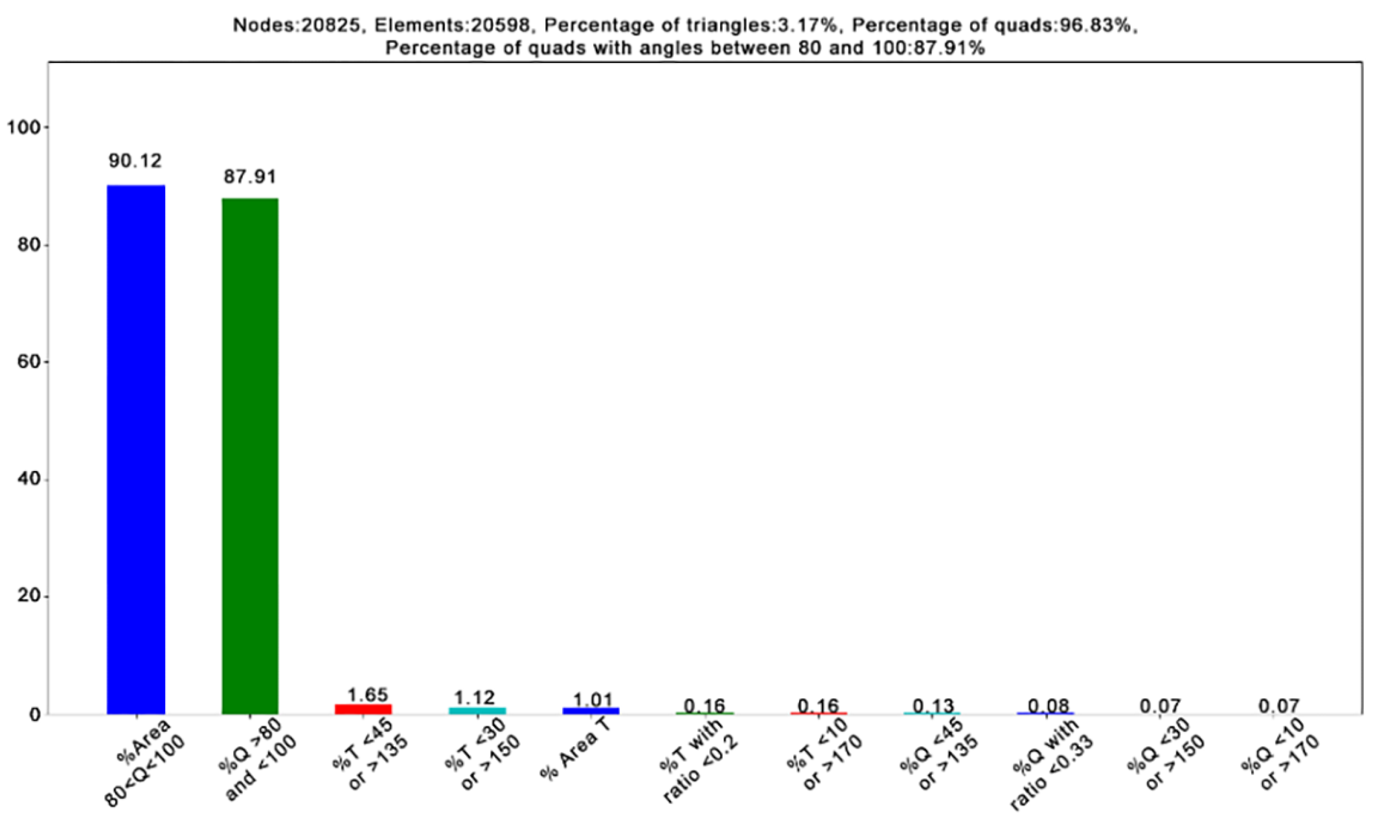
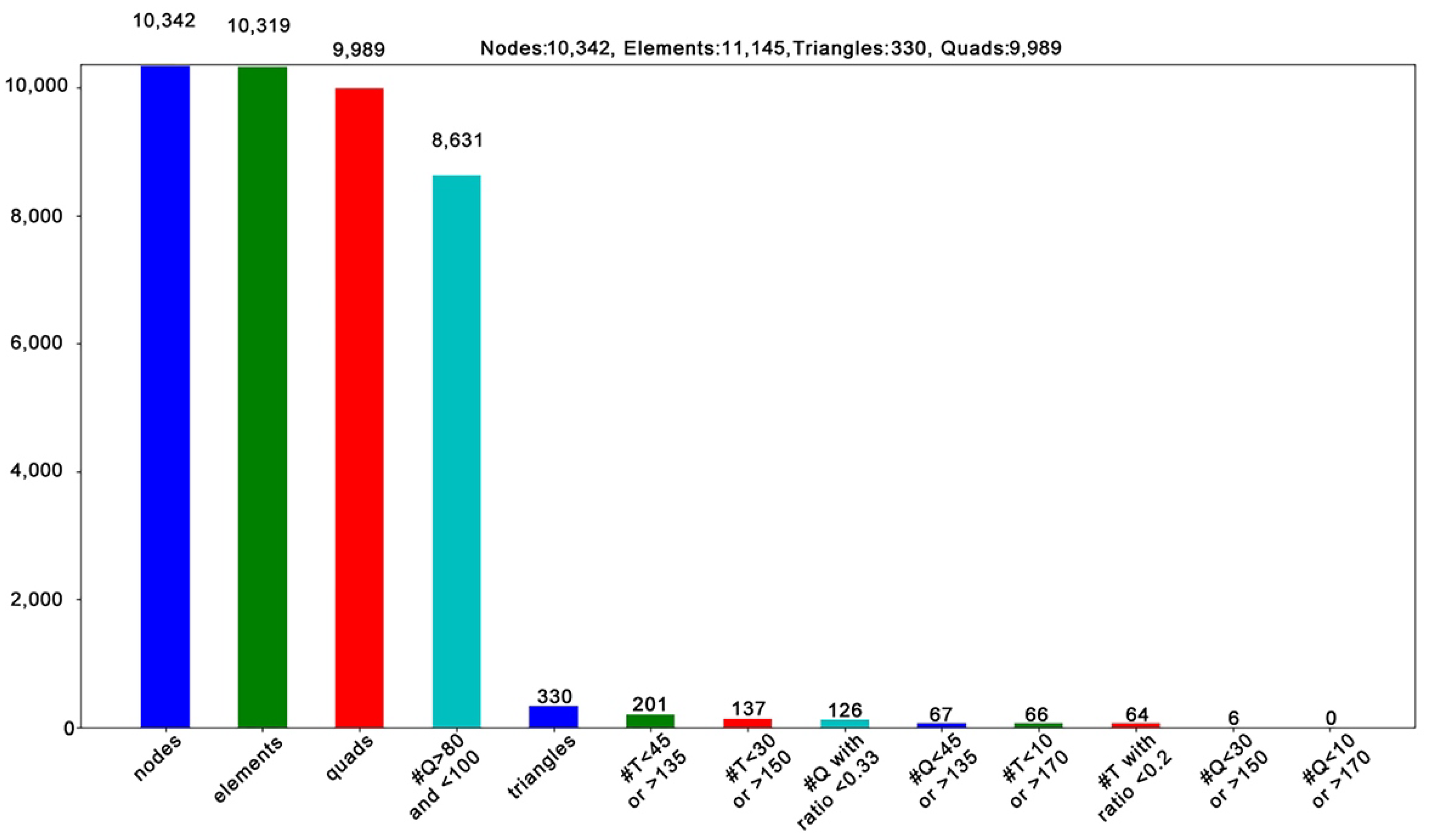
We assessed the quality of the mesh based on the statistics of the key performance indicators. Those are the values of the $\eta$ parameter which describe the local regularity of the mesh. A further performance measure is based on comparing the statistics for the gross number of elements (quads or triangles). We see that there are 3% triangles in the mesh and that 87% of elements are regular quadrilaterals. Those are quadrilaterals with the internal angles between 80° and 100°. Further analysis shows that the percentage of the surface area covered by regular elements is 90% (see Figure 14 representing statistics for the coarser mesh and Figure 15 representing statistics for the finer mesh).

A more informative consideration than an assessment of the statistical report is to consider where the problematic elements have appeared. The marching front quadrilateral Delaunay algorithm has pushed suboptimal elements (mostly triangles) to the boundary edges. In such a way, these elements could have been removed from the geometry in a modification of a geometric idealization procedure. This approach would incur problems of keeping the mesh connected while changing the model (possibly contrary to the wishes of a modeler). We claim, on the other hand, that it is better to leave the suboptimal elements on the boundaries of the model in the mesh. The perturbation which such elements cause to the stiffness matrix are such that they can be controlled by the modern linear system solvers. The potentially cause bad conditioning of the stiffness matrix, but their influence on the overall quality of the solution is controlled by a successful pivoting algorithm. By this, we mean any rank revealing sparse pivoting strategy, [26]. In particular, we envisage the use of the threshold rook pivoting from [27], which has been identified as the best compromise between robustness and efficiency. Given the fact that we have focused on providing as coarse meshes as possible which satisfy the accuracy criteria, we are typically dealing with small- to mid-size sparse matrices. As these matrices originated from surface meshes, we expect that the fill in in the LDU decomposition will be moderate and that the ill-conditioning will be picked out by the thresholded rook pivoting.

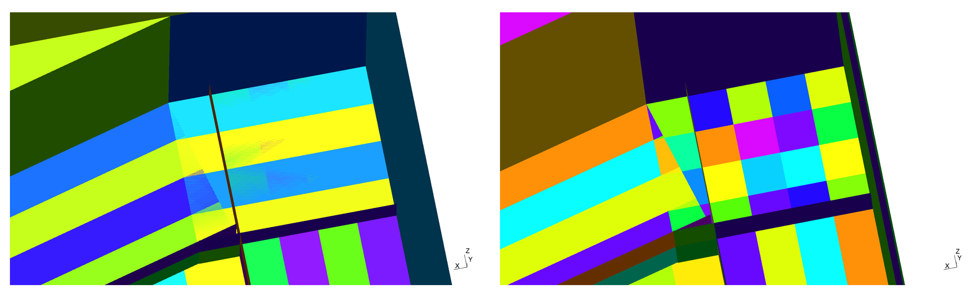
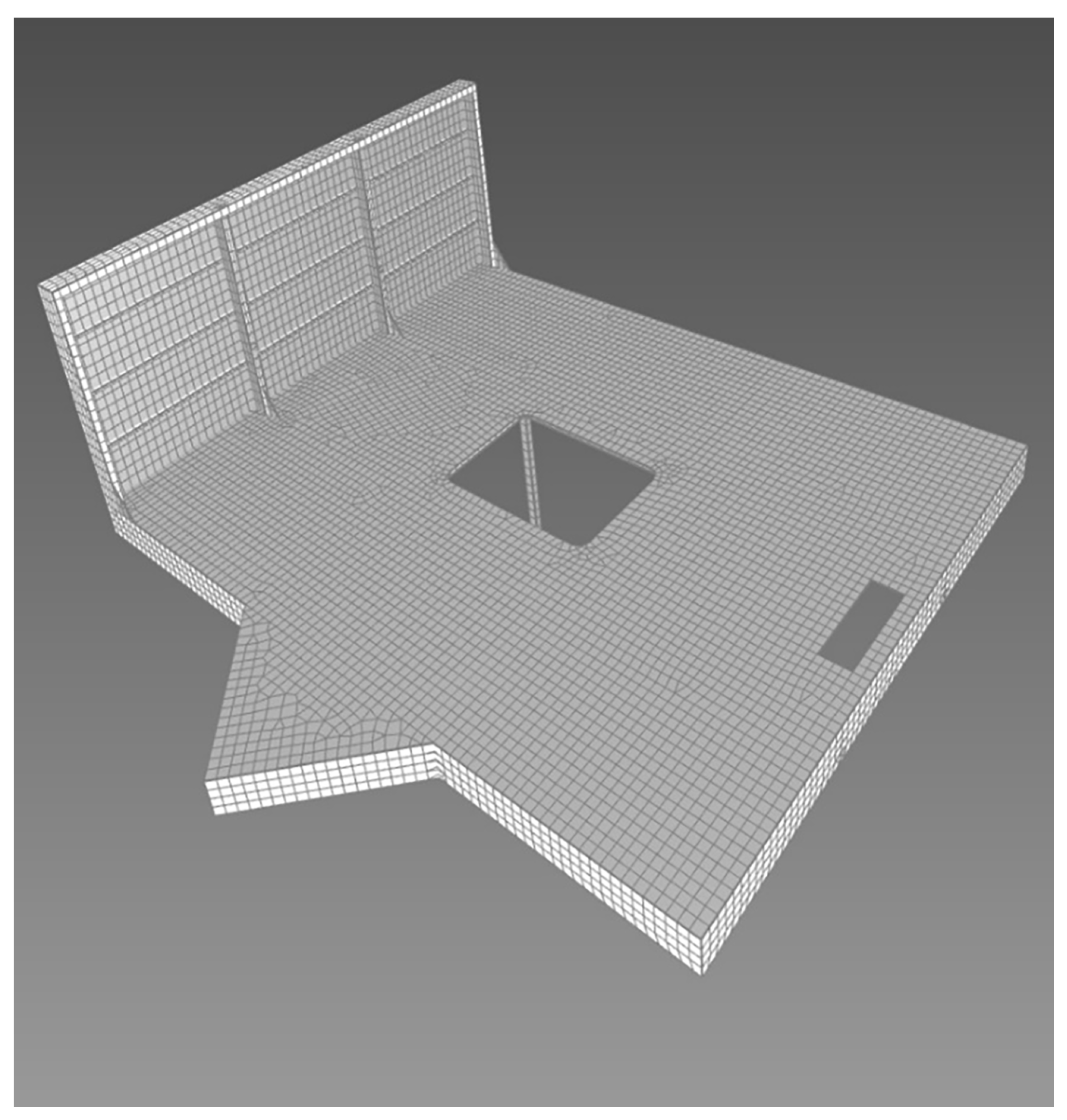
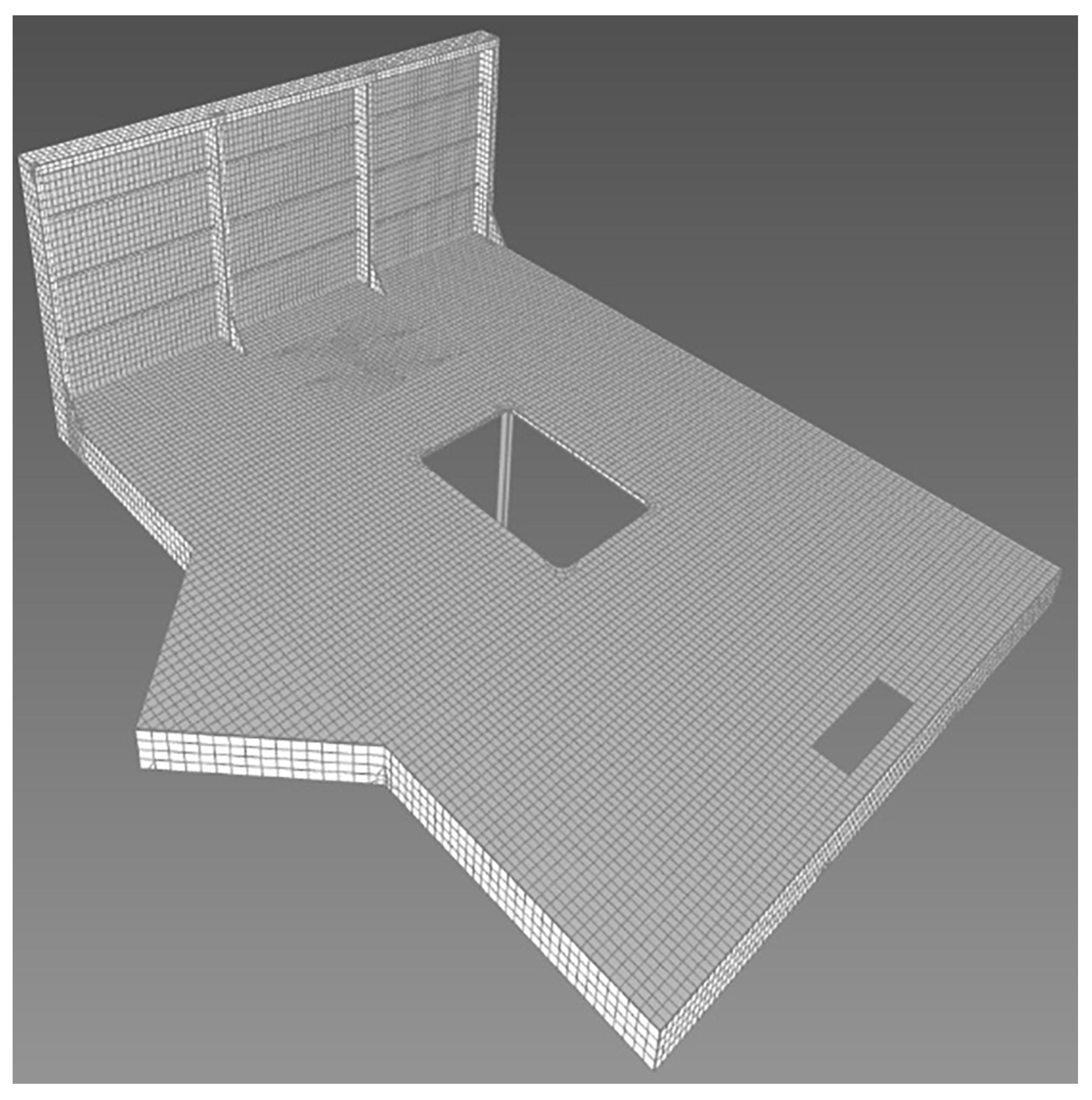
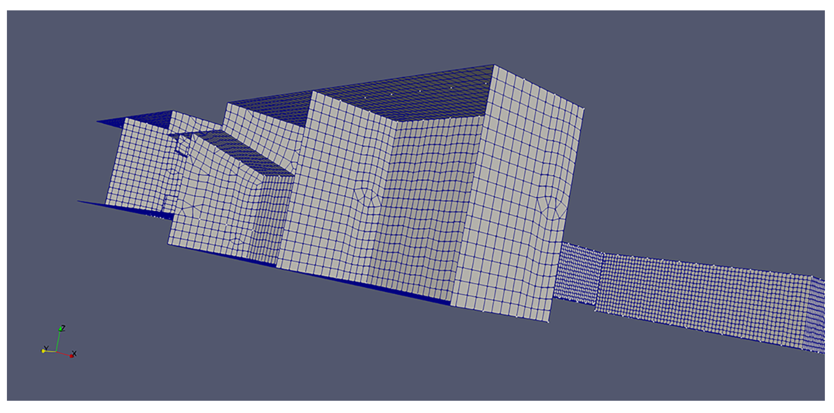
Finally, let us point out that an interactively generated mesh had 63% more degrees of freedom (at 18,481 elements). Furthermore, while manually generating the mesh, or when using the interactive mesh generation approach, the geometry is idealized by a modelers’ intervention and so a general comparison of the quality of mesh is hard. Should we compare the original or idealized/structured geometry? Based on the optimality of the perfect matching algorithm, we claim that it is not possible to generate a mesh by hand which will mesh the original geometry and have fewer than 12,000 elements. Note that in the automatically generated mesh in Figure 8 we clearly see a line of the gradual transition between advancing fronts of the quadrilateral elements. A gradual transition is achieved by a continuous transformation of a quadrilateral from a square to a slightly distorted trapeze (having angles in the span 80° to 100°). In comparison, the interactively generated mesh in Figure 9 has sharper transitions (a couple of more degenerate quadrilaterals or triangles) which accumulate the change needed to compensate for the consistent use of squares wherever possible. The meshing algorithm completed the automatic meshing task in under 10 s, whereas generating the mesh interactively requires expert engineering work. This is our main rationality for proposing the current solution.

If the comparison is to be made on the solution of a finite element study (statical/vibrational) then the influence of the triangles pushed to the boundary of the model on the accuracy of the assembled stiffness matrix is comparable with a similar perturbation of the boundary and should be accepted. This will be the subject of a separate numerical linear algebra analysis and is outside the scope of this paper.

Finally, let us compare the mesh generated by the automatic (batch) algorithm with the interactively generated mesh. The interactive algorithm allows for the full control of the mesh quality and produces a bespoke mesh (after many hours of expert work) which strictly satisfies the linear requirements, Figure 9. On the other hand, the fully automatic algorithm which starts from the uncleaned CAD geometry is able to generate a mesh with 30% fewer elements and the mesh satisfies the constraints in the statistical sense, Figure 8. This means that we interpret the optimization instruction to avoid triangles as a goal to keep the overall number of triangles below 5%. Note that almost 80% of the mesh is covered by regular quadrilaterals and that this mesh still satisfies the requirements of the classification societies for a coarse mesh model. Furthermore, when the geometry is updated by a designer searching for a design solution in the early phases of the design work, it can be easily be remeshed.

5. Conclusions

We have implemented a fully automatic processing pipeline for producing a quad dominated mesh for class-compliant ship structural analysis (see Figure 4). The mesh is generated to be suitable for the purposes of structural optimization or for early stages of the design process. The pipeline consists of three algorithms. First, we present an algorithm based on the Boolean operations with a tolerance. The algorithm is designed to correct the connectivity errors, solve the overlap problems for the elements of the geometry dictionary and to introduce obligatory points into the mesh. Such points could be the control or loading points, and they need to be retained in any mesh generated for a geometry. Second, we present the virtual stiffener algorithm which is used to control the local orientation of the mesh (cross-field) on web surfaces. Finally, last algorithm (Algorithm 1) in the pipeline is the adaptive sizing algorithm for web surfaces which is used to implement the classification society’s restrictions on the size of the mesh. We compare the results of our fully automatic mesh generation (see Figure 8) with the mesh generated interactively by an expert modeler (Figure 9). The automatic mesh has 97% of class compliant elements as opposed to 99% for the interactively generated mesh. However, the automatically generated mesh was produced without any user involvement in seconds. When assessing the results of the performance of the algorithm on other meshes, we propose that the method is fit for its declared purpose. Generating coarse meshes for use in optimization procedures and early stages of the design process.