Passive Sonar Target Tracking Based on Deep Learning

Abstract

At present, the tracking accuracy of underwater passive target tracking is often limited due to models that are overly simple, with low complexity, poor universality, and an inability to learn. In this paper, a cubature Kalman filter (CKF) algorithm based on a gated recurrent unit (GRU) network is proposed. The filter innovation, prediction error, and filter gain obtained from the CKF are used as the input to the GRU network, and the filter error value is used as the output to train the network. End-to-end online learning is carried out using the designed fully connected network, and the current state of the target is predicted. In this paper, a deep neural network based on the GRU architecture is used to convert the tracking prediction problem into a time series prediction problem in the field of artificial intelligence, and its strong fitting ability is used to resolve the uncertainty of the target motion. Simulation results show that an unmanned underwater vehicle (UUV) state estimation method based on the GRU filter proposed in this paper offers better accuracy and stability than the traditional state estimation method.

1. Introduction

Passive sonar is one of the main target detection methods for modern warships, submarines, unmanned underwater vehicles (UUVs), and so on [1]. Compared with active target tracking, passive target tracking has good concealment and high security. However, because it can only obtain the azimuth information of the target and has a long convergence time, its tracking accuracy is affected. Therefore, conducting in-depth research to improve tracking performance is essential. The principle of passive target tracking is to use sensors to passively measure the angle information of the target [2] and estimate the rule governing the variation in the motion parameters of the target with time in real time so as to establish and predict the course and trend of the motion state of the target. In essence, this is a nonlinear parameter estimation problem based on a filtered target state transition model used for prediction. At present, there are two main emphases of research on passive target tracking: improving the filtering algorithm and accurately describing the motion state of the target.

Passive target tracking is, in essence, a problem of nonlinear state estimation. Therefore, the commonly used nonlinear estimation methods mainly include the extended Kalman filter (EKF) [3,4], the unscented Kalman filter (UKF) [5,6,7], particle filters (PFs) [8,9,10], and the cubature Kalman filter (CKF) [11,12,13]. Because the measurement equation in passive target tracking contains only azimuth parameters, the system covariance matrix is prone to being negative definite in nature, resulting in filter divergence, which prevents stable tracking of the target. The authors of [14] took the azimuth change rate, the distance change rate, and the reciprocals of the azimuth and distance as state variables and proposed a modified polar extended Kalman filter (MPEKF) in a modified polar coordinate system, thereby effectively avoiding the possibility of a negative definite covariance matrix in the traditional EKF algorithm. Sun et al. [15] proposed a new augmented ensemble Kalman filter (AEnKF), which overcomes the limitations of linear measurement update rules in the framework of the linear minimum mean square error (LMMSE). However, the EKF algorithm is easily affected by initialization information, which may lead the tracking results to diverge or produce an ill-conditioned covariance matrix. The UKF algorithm [16] works with the actual nonlinear model and uses a minimum set of sample points to approximate the distribution function of the system state. Theoretically, it can capture the posterior mean and variance of any nonlinear function up to second order, making it especially suitable for solving higher-order nonlinear problems. Mehrjouyan et al. [17] proposed a robust adaptive unscented Kalman filter (RAUKF) for bearings-only tracking in three-dimensional cases (3DBOT). It combines the robustness of the UKF with the adaptability of the covariance matrix of the measurement noise, thereby improving the performance of the traditional UKF under an unknown noise covariance matrix and the errors caused by poor initial conditions. The complexity of the calculation is also reduced. Arasaratnam [18] used the third-order spherical radial rule to approximate the posterior distribution of states in order to solve the problem of filtering accuracy reduction or divergence in the UKF when solving a high-dimensional nonlinear state estimation problem. The CKF, which adopts the Gaussian filter equation in the Kalman filter structure, has better nonlinear approximation capabilities, numerical accuracy, and filter stability than the traditional UKF and EKF algorithms [19]. Leong et al. [20] combined the Gaussian mixture approach with the CKF to design a filter for bearings-only target tracking. Bearings-only tracking concerns a continuous–discrete system, with motion states in the continuous time domain and measurements in the discrete time domain. Because the CKF has higher estimation accuracy and fewer adjustable parameters than the UKF, it began to be applied to state estimation problems in many fields as soon as it was proposed. In many filtering methods, unpredictable approximation errors are inevitable due to the integration, discretization, and linearization of continuous models. To solve such problems, an adaptive covariance feedback framework has been proposed [21]. This framework is combined with a continuous–discrete volume Kalman filter to obtain the a priori covariance by using a posteriori covariance information. The covariance update is separated from the complex mathematical calculation; this can avoid unpredictable errors and improve the efficiency and accuracy, but significant changes in covariance will destroy the feedback channel. Based on the characteristics of cubature transformation, Zhang et al. [22] proposed a novel strong tracking CKF using the third-order information of the residual Taylor sequence expansion extracted by means of an attenuation factor. For different degrees of nonlinearity of the measurement function, this method demonstrates the superiority of introducing a fading factor.

Depending on the number of basic target state transition models used, target motion state prediction methods can be divided into single-model prediction methods and multi-model prediction methods. Single-model prediction methods are based on a single target state transition model. The commonly used basic target state transition models include the uniform speed model [7,23,24,25], the cooperative turning model [6,26,27], the constant acceleration model [28], the Singer model [29], and the current statistical model [30]. Multi-model prediction methods are based on multiple target state transition models. Depending on the matching degree between each model and the actual motion mode of the target, the single best-matching model may be used for prediction [31,32,33,34], or multi-model weighted prediction may be applied [35,36,37,38]. Reference [39] combined the EKF and UKF algorithms with the interactive multi-model (IMM) algorithm, analyzed the tracking performance of a bistatic passive tracking system, and verified through simulation that the IMM–UKF algorithm offers better stability when the system measurement error is large. Kim [40] proposed a filter restart strategy that tracks a maneuvering target by means of a constant speed observer under unequal speed constraints. When the filter is restarted, the stored target information can be reused by running the filter backward. Katsikas [41] applied a genetic algorithm to multiple models to design a genetic algorithm for online dynamic monitoring. Its structure changes with dynamic changes in the model, and a properly designed genetic algorithm is used to solve the model online. A variable structure multi-model algorithm based on directed graph switching and the UKF algorithm was proposed in [42]. Depending on the motion state of the target at different times, it matches different submodel sets according to the directed graph for filtering. Simulation results showed that this algorithm can effectively reduce the amount of calculation and make the model set better match the motion state of the target, thereby improving the tracking accuracy. Based on the monitoring and tracking of maneuvering maritime targets, focusing on strong maneuverability of the target and strong nonlinearity of the tracking system, Li et al. [43] established the IMM–SCKF algorithm by combining the IMM algorithm with the square root cubic Kalman filter (SCKF). Simulation results verified the accuracy of this algorithm in accurately identifying the time of a change in the motion pattern of the target. A new improved interactive multi-model particle filter (IMMPF) algorithm based on a mixed Gaussian flicker noise model was proposed in [44]. Simulation results showed that it exhibits a fast convergence speed and a strong adaptive ability, allowing it to better meet real-time tracking requirements for highly maneuverable targets.

In summary, the closer the established mathematical model is to the real motion mode of the target, the better the tracking effect will be. However, in practice, due to the unknown nature of the target motion, both the single-model and multi-model prediction methods discussed above face various problems, such as overly simple models, limited capabilities, and insufficient generalization. Although many filtering algorithms and improved methods have been proposed, it is still challenging to obtain accurate state estimation results due to the complexity and strong coupling of UUV dynamics and the inaccuracy of passive sonar measurements.

In recent years, due to its powerful feature expression ability, deep learning has achieved amazing results in natural language processing [45], image recognition [46,47], and other fields. At the same time, a large number of target tracking algorithms based on deep learning have emerged. An increasing number of tracking algorithms based on deep learning have achieved better performance than traditional tracking algorithms. Milan et al. [48] tried to determine the deformation state and controller coefficient of quadrotor with SPSA, and obtained the change of moment of inertia under deformation through a deep neural network. Then, in [49], several deformation states of hexarotor were obtained by using a deep neural network to estimate the moment of inertia and proportional integral derivative (PID) coefficient. The authors of [50] proposed a recurrent neural network (RNN) algorithm that can accomplish multitarget tracking tasks such as prediction, data association, state updating, target initiation, and termination under a unified network structure. The main advantage of this algorithm is that it is model free and does not require any prior knowledge about the target dynamics or clutter distribution. However, due to the simple structure of this algorithm, the potential of RNNs in dealing with uncertainty of the target motion is not given full play, and its tracking performance cannot meet the requirements [51]. The method of applying long short-term memory (LSTM) to solve complex and artificial long-term lag tasks was first proposed by Hocheriter et al. [52]. Kim et al. [53] combined LSTM with a residual framework to propose the Residual LSTM (RLSTM) algorithm for target tracking. Because the LSTM architecture alleviates the gradient disappearance problem of traditional RNNs in long time series, it has been applied in the field of sequence prediction. Gao et al. [54] proposed a method for addressing the uncertainty of the target motion based on a deep neural network for target tracking. Experiments proved that this method can better deal with uncertain target motion and offers better estimation accuracy. The gated recurrent unit (GRU) structure was proposed in 2014 [55]. Both GRU and LSTM are variants of RNN that can solve the problem of gradient disappearance in RNN when faced with long time series and thus have been widely used for sequence prediction. A GRU deep neural network achieves an effect similar to that of an LSTM deep neural network while having a simpler structure. A GRU network was constructed to capture the dynamic characteristics of tracking error in [56]. The tracking error is predicted by a trained neural network and compensated to a reference value in a feed-forward control structure, and good tracking performance is obtained. Hu et al. [57] proposed a hybrid algorithm based on the GRU structure and an IMM adaptive robust CKF. Experimental results validated its tracking error prediction ability and transient/steady state tracking performance.

To overcome the limitations of both traditional research methods and the latest deep learning theories and models in the field of sequence prediction, a CKF algorithm based on a GRU network (GRU–CKF) is proposed in this paper. GRU neurons are taken as the basic units to construct a multilevel neural network structure. The filter innovation, prediction error, and filter gain obtained from the CKF are used as the input to the GRU neural network, and the filter error value is used as the output to train the network. The trained GRU neural network is then used to compensate the filter state estimate of the CKF to obtain a new estimated state. Simulation results show that compared with traditional filter-based tracking methods (UKF, PF, and CKF), the proposed method offers better accuracy and stability.

2. Passive Sonar Target Tracking System Model

Unlike an active measurement system, a passive sonar system does not emit electromagnetic waves. It detects a target by receiving a radiation signal produced by the target itself or an external irradiation signal reflected by the target. Theoretically, two sensors can determine the unique position of a target in space when the measurement angle and the distance between them are known [58]. Therefore, a double observation station is used for real-time target tracking in this paper. As shown in Figure 1, the position of sensor 1 is taken as the origin of the coordinate system, the connecting line between sensors 2 and 1 is regarded as the X-axis, and the distance between the two sensors is L meters.

2.1. Target State Equation

The process of target motion can usually be described by the Markov state equation:

$${\mathrm{x}}_k=f_{k/k-1}\left(x_{k-1}\right)+w_k$$

(1)

Here, ${\mathrm{x}}_k={\left(x_k,y_k,{\dot{x}}_k,{\dot{y}}_k\right)}^T$ represents the target state vector, which usually contains the position, speed, and other information of the target. $f_{k/k-1}(•)$ represents the state transition function of the target from time $k-1$ to time $k$. $w_k$ represents the Gaussian noise in the target state: $w_k\sim N\left(q_k,Q_k\right)$.

2.2. Target Measurement Equation

The measured passive bistatic equation at time $k$ is:

$$z_k{=h}_k\left(x_k\right)+v_k$$

(2)

Here, $h_k={\left({\theta }_{{}_k}^{\left(1\right)},{\theta }_{{}_k}^{\left(2\right)}\right)}^T$ represents the measurement vector of the sensor and $v_k$ represents the Gaussian noise in the observation of the target: $v_k\sim N\left(r_k,R_k\right)$. The azimuth ${\theta }_{{}_k}^{\left(n\right)}$ measured by sensors 1 and 2 is calculated as follows:

$${\theta }_{{}_k}^{\left(1\right)}=\arctan \left(△y_k^{\left(n\right)}/△x_k^{\left(n\right)}\right)$$

(3)

$${\theta }_{{}_k}^{\left(2\right)}=\arctan \left[\left(△y_k^{\left(n\right)}-L\right)/△x_k^{\left(n\right)}\right]$$

(4)

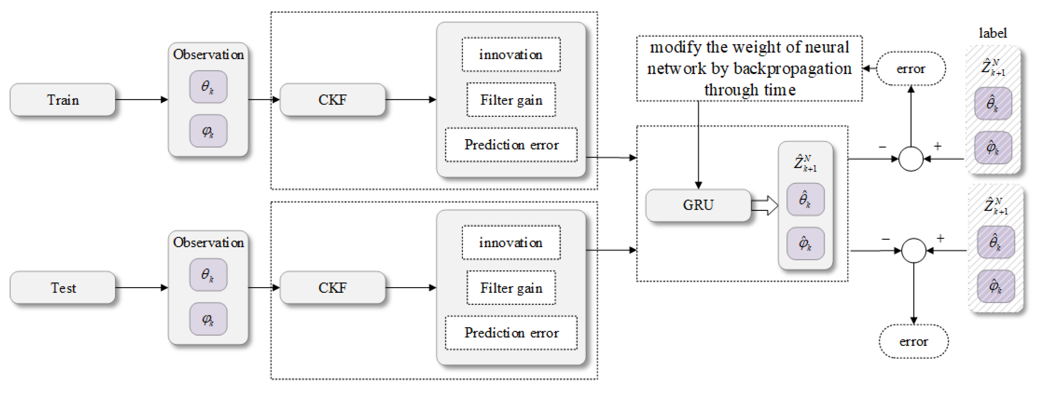
3. Passive Target Tracking Method Based on GRU–CKF

Underwater passive target tracking mostly relies on angle information, and there is a strong nonlinear relationship between observation and state, which leads to a nonlinear filtering problem. To solve a nonlinear filtering problem with a Gaussian distribution, it is necessary to solve the integral of the posterior expectation. As shown in Equation (5), the integrated function is the product of the nonlinear posterior distribution and a Gaussian probability density, and it is generally difficult to obtain an analytical solution.

$$I\left(f\right)={\displaystyle \underset{{ℝ}^n}{\int }f\left(x\right)\exp \left(-x^{T}x\right)dx}$$

(5)

Here, $f(•)$ is a nonlinear function, ${ℝ}^n$ is a ${}^n$ dimensional integral domain, and ${}^x$ is an integral vector.

The CKF algorithm is based on the third-order spherical radial cubature criterion and uses a set of equal weight cubature points to approximate the posterior probability density of the target state. Equation (6) is the integral formula for calculating the Gaussian weight.

$$I_N\left(f\right)={\displaystyle \underset{{ℝ}^n}{\int }f\left(x\right)N\left(x;\mathbf{0},I\right)dx\approx {\displaystyle \sum _{i=1}^m{\omega }_{i}f\left({\xi }_i\right)}}$$

(6)

Here, ${\xi }_i=\sqrt{\frac{m}{2}}{\left[1\right]}_i=\sqrt{\frac{m}{2}}{\left\{\left(\begin{array}{c}1\\ ...\\ 0\end{array}\right),...,\left(\begin{array}{c}0\\ ...\\ 1\end{array}\right),\left(\begin{array}{c}-1\\ ...\\ 0\end{array}\right),...,\left(\begin{array}{c}0\\ ...\\ -1\end{array}\right)\right\}}_i,{\omega }_i=\frac{1}{m},i=1,2,...,m=2n$ is the dimensionality of the system state vector, and ${}^n$ is the point set in [1] dimensional space.

It can be seen from the above process that the CKF uses $2n$ equal weight cubature points to calculate complex integrals and requires statistical methods to complete the time update and measurement update in the filtering cycle.

3.1. Time Update

Under the assumption that the posterior state probability density function $p\left(x_{k-1}\right)=N\left({\widehat{x}}_{k-1|k-1},P_{k-1|k-1}\right)$ at $k-1$ is known, Cholesky decomposition is performed on the estimation error covariance $P_{k-1|k-1}$:

$$P_{k-1|k-1}=S_{k-1|k-1}{S}_{k-1|k-1}^{\mathrm{T}}$$

(7)

Calculated Cubature points:

$$X_{i,k-1|k-1}=S_{k-1|k-1}{\xi }_i+{\widehat{x}}_{k-1|k-1}$$

(8)

The predicted value of the Cubature point is calculated by using the equation of state:

$$X_{i,k|k-1}^{\ast }=f\left(X_{i,k-1|k-1}\right)$$

(9)

Here, $i=1,2,\dots ,m$

Estimate the state prediction value at $k$:

$${\widehat{x}}_{k|k-1}=\frac{1}{m}{\displaystyle \sum _{i=1}^m{X}_{i,k|k-1}^{\ast }}=\frac{1}{m}{\displaystyle \sum _{i=1}^{m}f\left(X_{i,k-1|k-1}\right)}$$

(10)

It is estimated that the predicted value of state error covariance at $k$ time is:

$$P_{k|k-1}=\frac{1}{m}{\displaystyle \sum _{i=1}^m{X}_{i,k|k-1}^{\ast }}{X}_{i,k|k-1}^{\ast \mathrm{T}}-{\widehat{x}}_{k|k-1}{\widehat{x}}_{k|k-1}^{\mathrm{T}}+Q_{k-1}$$

(11)

3.2. Measurement Update

Cholesky decomposition of $P_{k|k-1}$:

$$P_{k|k-1}=S_{k|k-1}{S}_{k|k-1}^{\mathrm{T}}$$

(12)

Calculate the Cubature points of the predicted value of the state:

$$X_{i,k|k-1}=S_{k|k-1}{\xi }_i+{\widehat{x}}_{k|k-1}$$

(13)

Propagate the Cubature points through the measurement equation:

$$Z_{i,k|k-1}=h\left(X_{i,k|k-1}\right)$$

(14)

Estimated measured predicted value at $k$:

$${\widehat{z}}_{k|k-1}=\frac{1}{2n}{\displaystyle \sum _{i=1}^{2n}{Z}_{i,k|k-1}}=\frac{1}{2n}{\displaystyle \sum _{i=1}^{2n}h\left(X_{i,k|k-1}\right)}$$

(15)

Calculate the measurement autocorrelation error covariance matrix:

$$P_{zz,k|k-1}=\frac{1}{2n}{\displaystyle \sum _{i=1}^{2n}{Z}_{i,k|k-1}}{Z}_{i,k|k-1}^{\mathrm{T}}-{\widehat{z}}_{k|k-1}{\widehat{z}}_{k|k-1}^{\mathrm{T}}+R_k$$

(16)

Calculate the cross-correlation covariance matrix:

$$P_{xz,k|k-1}=\frac{1}{2n}{\displaystyle \sum _{i=1}^{2n}{X}_{i,k|k-1}{Z}_{i,k|k-1}^{\mathrm{T}}}-{\widehat{x}}_{k|k-1}{\widehat{z}}_{k|k-1}^{\mathrm{T}}$$

(17)

Calculate Kalman gain:

$$K_k=P_{xz,k|k-1}{P}_{zz,k|k-1}^{-1}$$

(18)

Calculate the estimated value of the system state at $k$:

$${\widehat{x}}_{k|k}={\widehat{x}}_{k|k-1}+K_k\left(z_k-{\widehat{z}}_{k|k-1}\right)$$

(19)

Calculate the estimated value of state error covariance matrix at $k$:

$$P_{k|k}=P_{k|k-1}-K_k{P}_{zz,k|k-1}{K}_k^{\mathrm{T}}$$

(20)

When the system is in a stable state, the filter gain $K_k$ tends to the minimum. At this time, if the target executes a sudden maneuver, the prediction error $\left({\widehat{x}}_{k|k-1}-{\widehat{x}}_{k|k}\right)$ increases, but the gain matrix remains at the minimum, which leads to divergence of the tracking results of the CKF algorithm. Therefore, the more complex the underwater environment is and the stronger the mobility of the target is, the more prominent the divergence of the CKF. Therefore, this paper proposes a passive tracking method based on a deep GRU neural network-assisted CKF. The GRU based neural network framework for time series expansion is composed of an input layer, a hidden layer, an intermediate layer, and an output layer, as shown in Figure 2. A GRU consists of an update gate $z_k$ and a reset gate $r_k$. $z_k$ determines the integration of newly input information and historical information, and $r_k$ determines the proportion of state information from the previous step that is integrated into the model. The forward calculation formula of a GRU is:

$${\tilde{S}}_k={\varphi }_{\tanh }\left(W_S\cdot \left(r_k\odot S_{k-1}\right)+U_S{x}_k+b_S\right)$$

(21)

$$S_k=\left(1-z_k\right)\odot S_{k-1}+z_k\odot {\tilde{S}}_k$$

(22)

$$z_k={\sigma }_{sig}\left(W_z{S}_{k-1}+U_z{x}_k+b_z\right)$$

(23)

$$r_k={\sigma }_{sig}\left(W_r{S}_{k-1}+U_r{x}_k+b_r\right)$$

(24)

Here, $\odot$ represents the element product formula; $W_z$ and $W_r$ are the weight matrices of $z_k$ and $r_k$, respectively; $W_S$ is the weight matrix of the output state; $x_k$ is the input data at $k$; ${\tilde{S}}_k$ and $S_k$ are the candidate states and output states, respectively, at $k$; $b_S$, $b_r$, and $b_z$ are constants; and ${\sigma }_{sig}$ and ${\varphi }_{\tanh }$ are the $sigmoid$ and $\tanh$ activation functions, which are used to activate the control gate and candidate states, respectively, and are expressed as $sig\left(x\right)=\frac{1}{1+e^x}$ and $\tanh \left(x\right)=2\ast sig\left(x\right)-1$. In the hidden layer, each GRU consists of a reset gate and an update gate. The reset gate combines new information with memory to help capture short-term information in the time series. The update gate determines the amount of memory information saved to the current time, which helps the GRU capture long-term correlation. In this way, GRUs can capture the features of time-related measurement information and model the mapping between the previous measurement of the target and the current state of the target.

As Figure 2 shows, the internal structure of the GRU neural network gradually expands over time. In this network, the input layer accepts the angle measurement information $\left\{{\theta }_k^1,{\theta }_k^2\right\}$ of the target at the previous time, the output layer produces the angle information $\left\{{\theta }_{k+1}^1,{\theta }_{k+1}^2\right\}$ of the target at the next time, and the hidden layer is composed of GRUs and is fully connected to the intermediate layer. The optimal number of hidden and middle layer neurons and the parameters are determined by the training data set and validation data set. In each time period, $k+1$, the measured value of the target at time $k$ is input to the network, and the effective eigenvalues from times $0:k-1$ are stored in the hidden layer. This structure increases the complexity between the hidden layer and the output layer to improve the sensitivity of the neural network parameters and the nonlinear expression ability of the model.

It can be seen from Equation (19) that the error between the updated state estimate value of the CKF and the accurate state is mainly affected by the innovation $\left(z_k-{\widehat{z}}_{k|k-1}\right)$, the prediction error $\left({\widehat{x}}_{k|k-1}-{\widehat{x}}_{k|k}\right)$, and the filter gain $K_k$. Therefore, based on the measured values from observation $k-1$ to $k$, the steps of passive target state estimation based on the GRU–CKF algorithm are as follows:

Step 1: Use the CKF process to collect the input data for the GRU network.

Taking the data from periods $0\to t_{k-1}$ as training data, the innovation $\left(z_k-{\widehat{z}}_{k|k-1}\right)$, prediction error $\left({\widehat{x}}_{k|k-1}-{\widehat{x}}_{k|k}\right)$ and filter gain $K_k$ obtained via the CKF method are used as the input to the GRU network. It can be seen from Equations (1) and (2) that the innovation $\left(z_k-{\widehat{z}}_{k|k-1}\right)$ is a one-dimensional vector, the prediction error $\left({\widehat{x}}_{k|k-1}-{\widehat{x}}_{k|k}\right)$ is a two-dimensional vector, and the filter gain $K_k$ is a two-dimensional vector. Therefore, the number of neurons in the input layer is 5, where the superscript * represents the input samples of training data from periods $0\to t_{k-1}$. At the same time, the error value $\left({\widehat{x}}_{k|k}-{\widehat{x}}_{k-1|k-1}\right)$ between the updated state estimate value ${\widehat{x}}_{k|k}$ and the accurate state value ${\widehat{x}}_{k-1|k-1}$ with the corresponding CKF method is taken as the output value of the GRU network. The dimensionality of the filtering error $\left({\widehat{x}}_{k|k}-{\widehat{x}}_{k-1|k-1}\right)$ is 2, so the number of neurons in the output layer is also 2. The connection weights between the hidden layer and the output layer of the GRU network are repeatedly trained based on these input and output values.

Step 2: Update the estimated state value through GRU-estimation-based filter error compensation.

By using the CKF method to filter and estimate the data in periods $t_k\to t_e$, we can obtain the innovation $\left(z_k-{\widehat{z}}_{k|k-1}\right)$, the prediction error $\left({\widehat{x}}_{k|k}-{\widehat{x}}_{k-1|k-1}\right)$, and the filter gain $K_k$ for the state update and take them as the input values for the GRU network after training to obtain the filter error $\tilde{X}$. By adding the estimated filter error $\tilde{X}$ output by the network to the filter estimated value ${\widehat{x}}_{k|k}$, we can obtain a new and more accurate state estimate. Based on the above steps, the passive sonar target tracking process of GRU–CKF is shown in Figure 3. This method based on GRU-assisted CKF utilizes the accuracy and stability of CKF estimation and the learning ability and speed of GRU to achieve a more accurate correction filter estimation value.

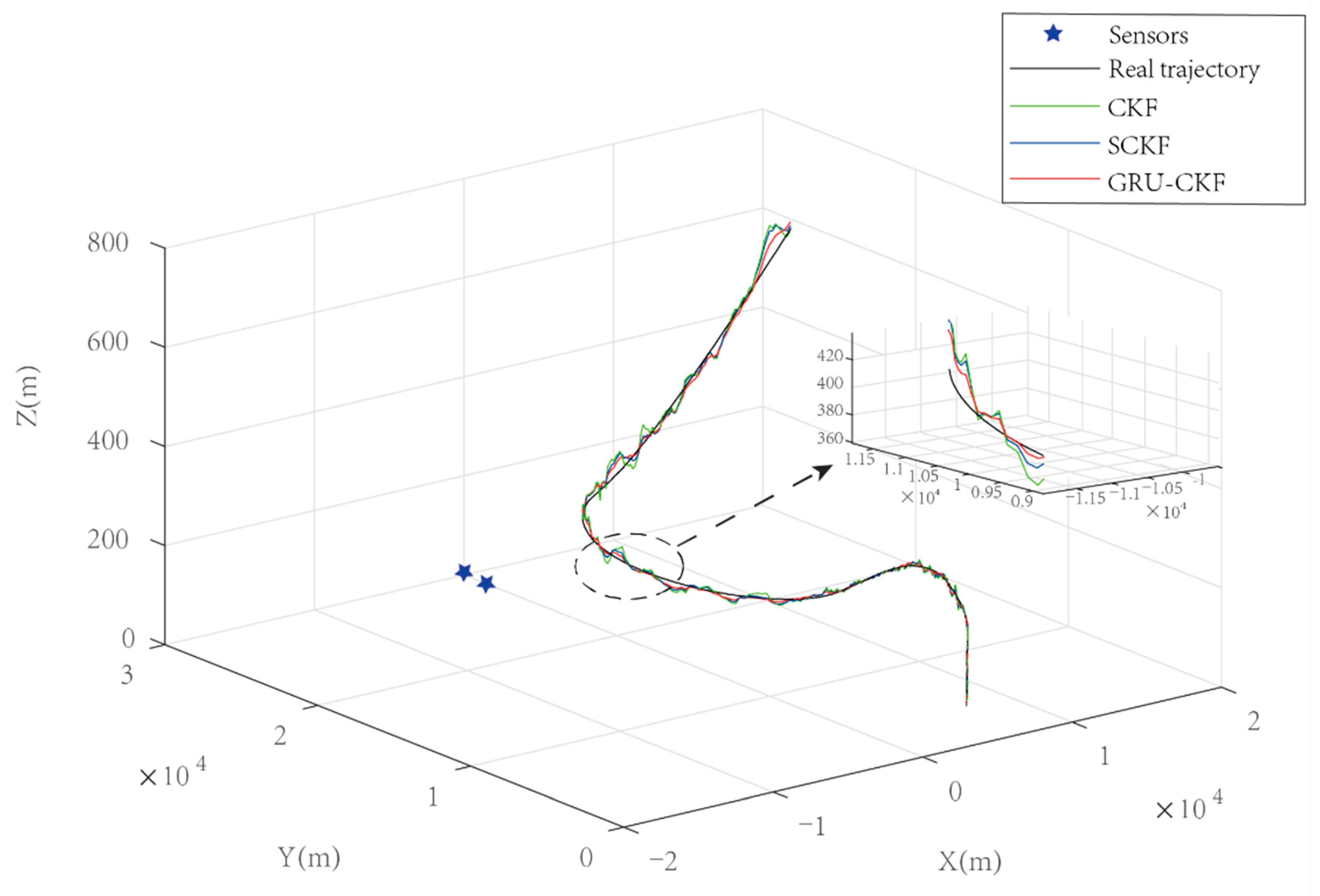
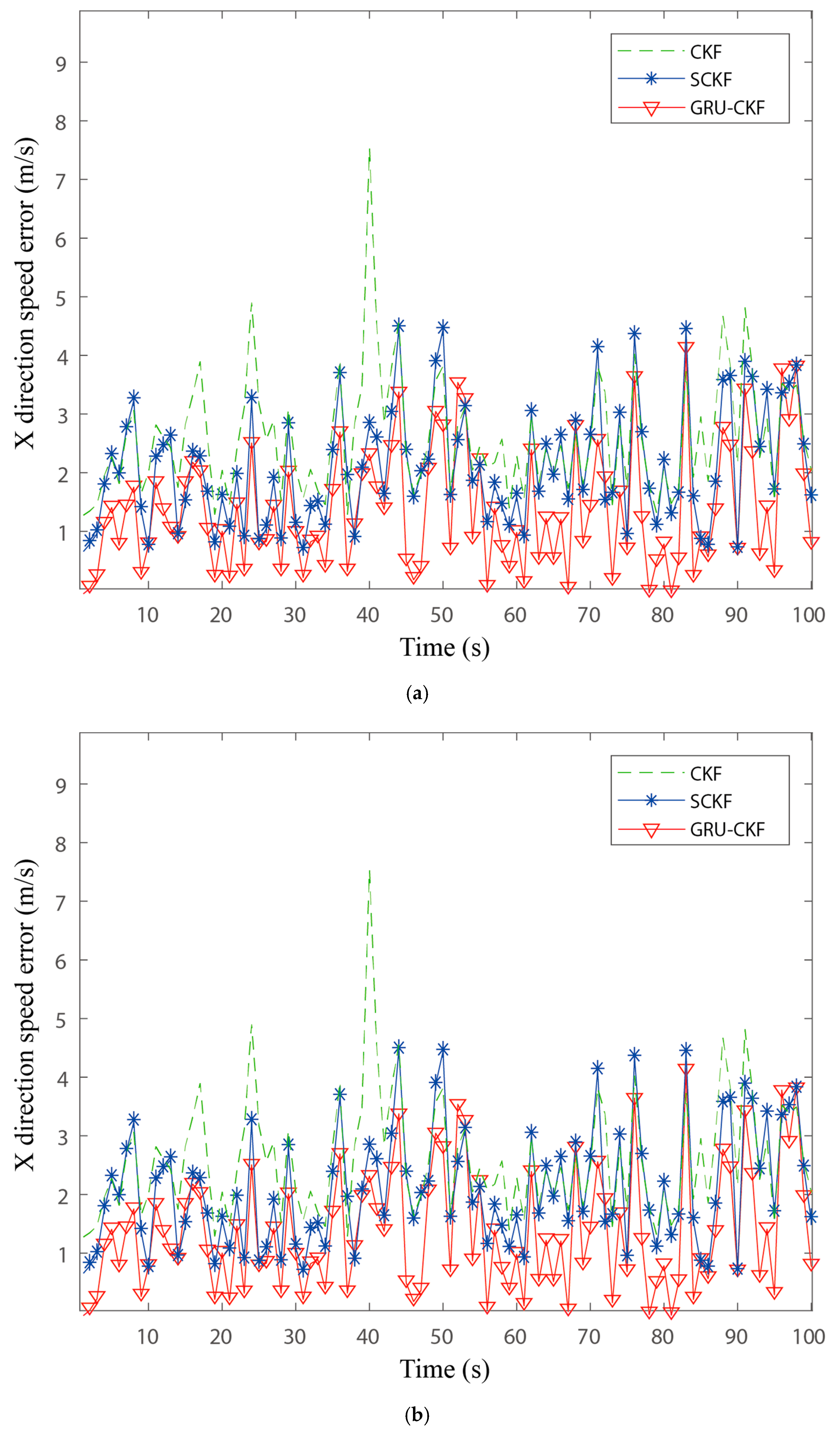
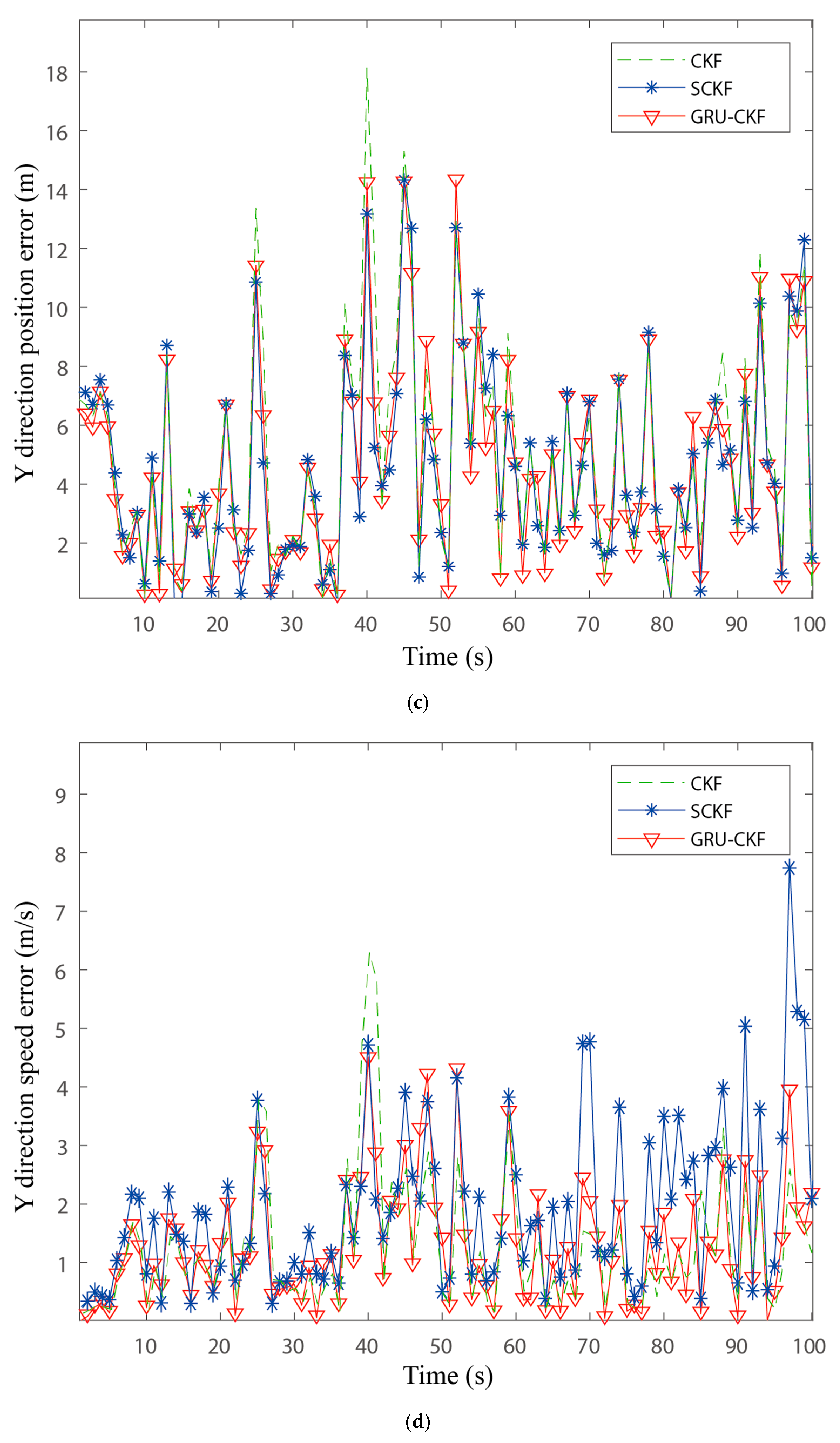
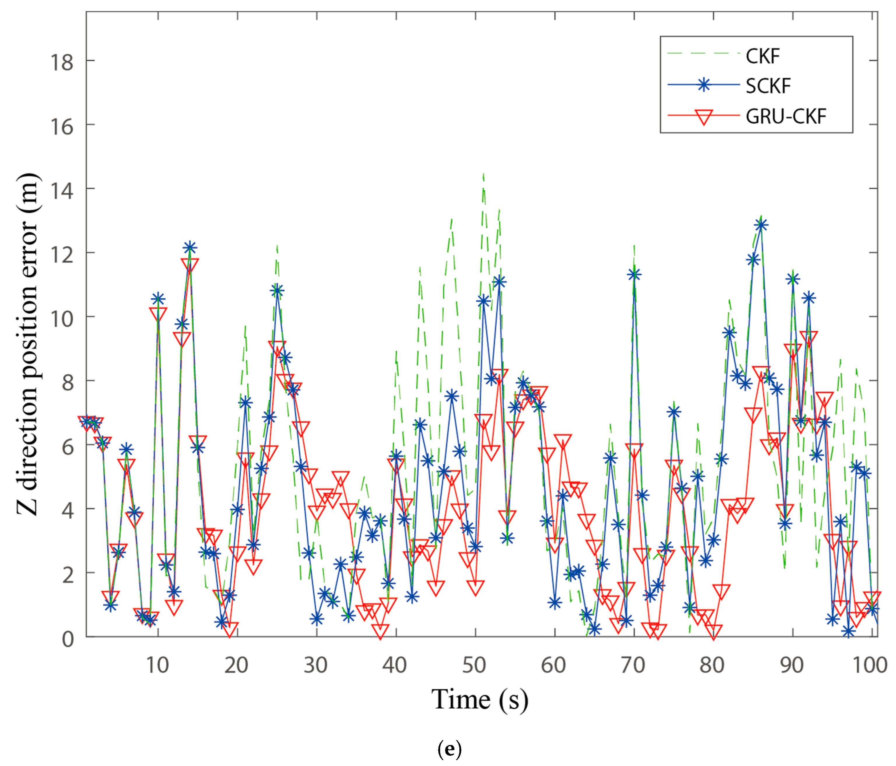
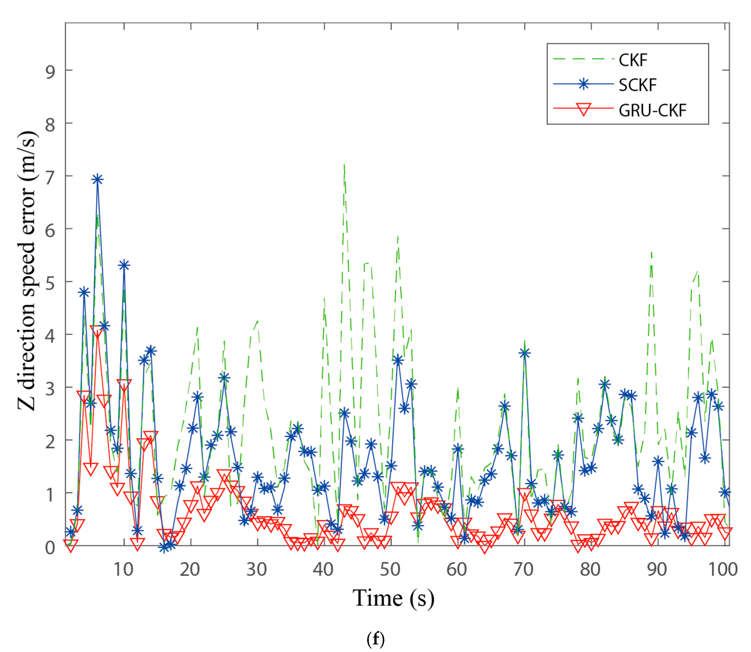
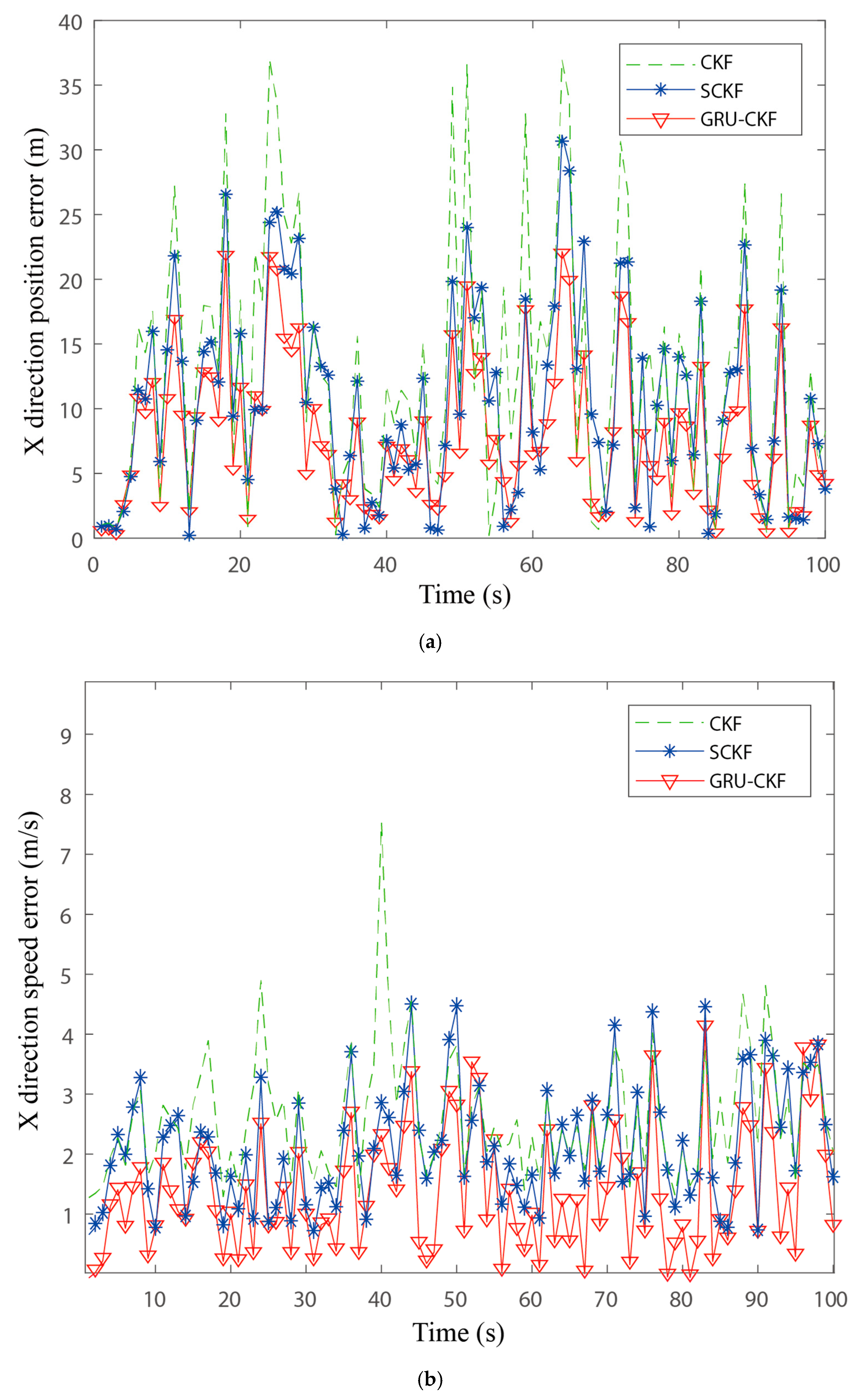
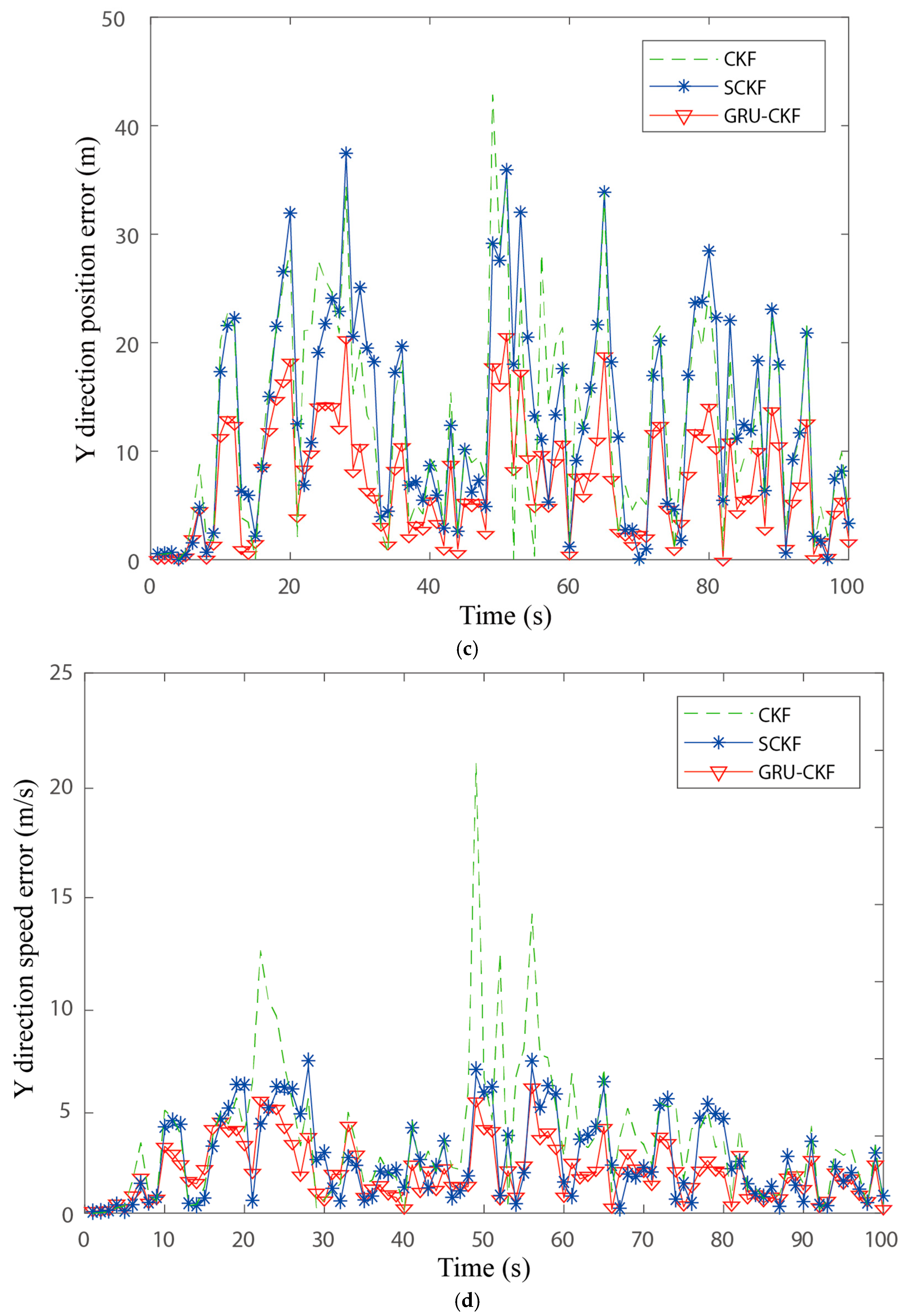
4. Simulation Results

Considering that in an actual environment, the target usually exhibits strong maneuvering and the maneuvering mode of the target is relatively complex, a general acceleration model cannot reasonably describe the form of the target motion. Therefore, this paper uses constant velocity (CV), constant acceleration (CA), and cooperative turning (CT) models to construct the target motion model, generate 4 sets of training samples, 2 set of test samples, and 1 set of test samples, with 400 samples in each set. The change in the motion state of the target in the test samples with time over time is expressed in

Table 1. Motion model design.

Time/s	Motion Model	Motion Parameters
0~50	CA	The accelerations in X, Y, and Z directions are set to: 0.5 m/s2, 0.4 m/s2, 0 m/s2
51~90	CV	The velocities in X, Y, and Z directions are set to: 25 m/s, −26 m/s, −15 m/s
91~170	CT	The angular velocity is set to: $\omega =2^{°}$
171~230	CA	The accelerations in X, Y, and Z directions are set to: −2 m/s2, −0.5 m/s2, −0.2 m/s2
231~320	CT	The angular velocity is set to: $\omega =-2^{°}$
321~400	CA	The accelerations in X, Y, and Z directions are set to: 2 m/s2, 1 m/s2, 0 m/s2

.

The position of one observation station is selected as the coordinate origin to establish the coordinate system. It is assumed that the coordinates of the two observation stations are $\left[0,0,0\right]$ and $\left[0,500,0\right]$, respectively.

The simulation duration is 400 s and the observation sampling period is 1 s.

The azimuth measurement variance is ${\sigma }_{1,2}^2={\left(0.1\times \left(\pi /180\right)\right)}^2\left({\mathrm{rad}}^2\right)$.

The number of Monte Carlo simulations is 50.

Select root mean square error (RMSE) as the standard to measure the predicted value and actual value:

$$RMSE(m,\stackrel{⌢}{m})=\sqrt{\frac{1}{N}{\displaystyle \sum _{i=1}^N{(m_i-{\stackrel{⌢}{m}}_i)}^2}}$$

(25)

where $m_i$ represents the actual value, ${\stackrel{⌢}{m}}_i$ represents the predicted value, and $N$ is the number of Monte Carlo simulations.

To analyze the performance of the GRU–CKF algorithm, it is compared with the CKF and SCKF algorithms in this section. Figure 4 shows the estimated target trajectories obtained using state estimation methods based on the CKF, SCKF, and GRU–CKF algorithms. It can be clearly seen from the estimated trajectories in Figure 4 that GRU–CKF achieves the best estimation performance in this scenario.

Figure 5 and Figure 6 show the root mean square errors (RMSEs) of the positions and velocities of the three methods in the X, Y, and Z directions with different measurement errors, respectively.

In addition, when other initial conditions are the same, consider increasing the azimuth measurement variance of the two observation stations by 10 times, and observe the tracking performance of the three algorithms under different measurement noise. Figure 6 shows the position error and velocity error of the three algorithms in all directions after the measurement variance of the observation station is expanded by 10 times.

As seen from Figure 5a–d, in the X and Y-axis directions, the RMSEs of the GRU–CKF and SCKF algorithms are similar in both position and velocity. As seen from Figure 5e,f, in Z-axis directions, compared with the other two methods, the GRU–CKF algorithm has the best RMSE in position and speed. After the measurement variance of the observation station is expanded by 10 times, the GRU–CKF algorithm has more obvious advantages with the other two methods, as shown in Figure 6, in the X, Y, and Z-axis directions, the GRU–CKF algorithm not only obtains the lowest position RMSE but also the most stable position RMSE. It can be seen from

Table 2. Stability and positioning accuracy of various algorithms.

Algorithm	${\mathit{\sigma }}_{\mathbf{1}\mathit{,}\mathbf{2}}^{\mathbf{2}}\mathbf{=}{\mathbf{\left(}\mathbf{0.1}\mathbf{\times }\mathbf{\left(}\mathit{\pi }\mathbf{/}\mathbf{180}\mathbf{\right)}\mathbf{\right)}}^{\mathbf{2}}\mathbf{\left(}{\mathbf{rad}}^{\mathbf{2}}\mathbf{\right)}$			${\mathit{\sigma }}_{\mathbf{1}\mathit{,}\mathbf{2}}^{\mathbf{2}}\mathbf{=}{\mathbf{\left(}\mathbf{0.5}\mathbf{\times }\mathbf{\left(}\mathit{\pi }\mathbf{/}\mathbf{180}\mathbf{\right)}\mathbf{\right)}}^{\mathbf{2}}\mathbf{\left(}{\mathbf{rad}}^{\mathbf{2}}\mathbf{\right)}$
	$\mathit{P}\mathit{M}\mathit{S}{\mathit{E}}_{\mathit{x}}$	$\mathit{P}\mathit{M}\mathit{S}{\mathit{E}}_{\mathit{y}}$	$\mathit{P}\mathit{M}\mathit{S}{\mathit{E}}_{\mathit{z}}$	$\mathit{P}\mathit{M}\mathit{S}{\mathit{E}}_{\mathit{x}}$	$\mathit{P}\mathit{M}\mathit{S}{\mathit{E}}_{\mathit{y}}$	$\mathit{P}\mathit{M}\mathit{S}{\mathit{E}}_{\mathit{z}}$
CKF	11.6104	11.3828	12.3102	26.3347	27.3653	15.0960
SCKF	9.4278	9.9950	9.9217	20.4412	21.2506	10.6005
GRU–CKF	6.6508	8.3904	7.2551	6.9011	8.6089	7.6733

that when the equivalent measurement error rises sharply, the stability of the GRU–CKF algorithm is better than the CKF and SCKF algorithm, and the relative position accuracy is basically consistent with that when the measurement error does not rise. It shows that the GRU–CKF algorithm has high stability. Even if the target suddenly changes its motion state or the measurement error rises sharply, it can still estimate the position of the target with high precision.

5. Conclusions

In this paper, the GRU–CKF algorithm is proposed to solve the problem of low accuracy of target state estimation caused by the strong nonlinear relationship between the pure angle measurement and the state in underwater passive target tracking and highly maneuverable target motion. First, the filter innovation, prediction error, and filter gain obtained from the CKF are used as the input to a GRU network, and the filter error value is used as the output. The connection weights between the hidden layer and the output layer of the GRU network are repeatedly trained, and then, the estimated state value is updated by means of filter error compensation based on the GRU estimation result. The GRU–CKF algorithm can identify and filter out nonlinear and uncertain measurement noise. The traditional methods of resolving uncertainty may lead to performance degradation and accuracy limitations. To study the performance of the proposed GRU–CKF algorithm, its estimation performance is compared with that of other state estimation methods based on the CKF and SCKF algorithms in various scenarios. The simulation results show that the proposed GRU–CKF method overcomes the limitations of the traditional model-based methods in terms of statistical estimation accuracy and handles uncertainty of the target motion well. However, due to the uncertainty and complexity of the underwater environment, the sensor may not work for a short time. To solve this kind of problem, further research and exploration are still needed.

References

1. Wang, Y.-K.; Ding, Y. Data Fusion Simulation Model of Passive Sonar Target Wake Tracing Based on MGEKF. Torpedo Technol. 2010, 18, 35–40. [Google Scholar]
2. Zhang, M.-T. Research on Fusion Algorithm of Multi Mobile Observations in Angle-Only Target Tracking. Master’s Thesis, Nanjing University, Nanjing, China, 2017. [Google Scholar]
3. Guan, X.; He, Y.; Yi, X. Emulational Analysis on the Performance of Underwater Bearing-only Passive Target Tracking Using Two Arrays. J. Syst. Simul. 2003, 15, 1464–1466. [Google Scholar]
4. Ito, M.; Tsujimichi, S.; Kosuge, Y. Tracking a three-dimensional moving target with distributed passive sensors using extended Kalman filter. Electron. Commun. Jpn. 2010, 84, 74–85. [Google Scholar] [CrossRef]
5. Cao, Z.Q.; Meng, H. Bearing-only tracking algorithm for underwater passive target. Electron. Des. Eng. 2014, 22, 74–76. [Google Scholar]
6. Xiao, B.-Q. Locating and Tracking of Target with Bearing-Only Small Maneuvering. Electron. Opt. Control 2017, 9, 27–30. [Google Scholar]
7. Wang, B.-B.; Wu, P.L. Underwater bearing-only tracking based on square-root unscented Kalman filter smoothing algorithm. J. Chin. Inert. Technol. 2016, 24, 180–184. [Google Scholar]
8. Xu, L.-X.; Liu, C.Y.; Yi, W.; Li, G.; Kong, L. A particle filter based track-before-detect procedure for towed passive array sonar system. In Proceedings of the 2017 IEEE Radar Conference (RadarConf), Seattle, WA, USA, 8–12 May 2017. [Google Scholar]
9. Tiwari, R.K.; Radhakrishnan, R.; Bhaumik, S. Particle Filter for Underwater Passive Bearings-Only Target Tracking with Random Missing Measurements. In Proceedings of the 2018 17th European Control Conference (ECC), Limassol, Cyprus, 12–15 June 2018. [Google Scholar]
10. Georgy, J.; Noureldin, A. Unconstrained underwater multi-target tracking in passive sonar systems using two-stage PF-based technique. Int. J. Syst. Sci. 2014, 45, 439–455. [Google Scholar] [CrossRef]
11. Liu, Y.-L.; Feng, X.-X. Multiple Passive Sensors Target Tracking Algorithm Based on CKF. Comput. Simul. 2013, 30, 189–193. [Google Scholar]
12. Dai, D.C.; Cai, Z.P.; Niu, C. Target Tracking Algorithm Based on Reduced Square-Root Cubature Kalman Filter. Electron. Opt. Control. 2015, 22, 11–14. [Google Scholar]
13. Xu, J.; Xu, M.Z.; Zhou, X.-Y. The Bearing Only Target Tracking of UUV based on Cubature Kalman Filter with Noise Estimator. In Proceedings of the 36th Chinese Control Conference, Dalian, China, 26–28 July 2017. [Google Scholar]
14. Hammel, S.; Aidala, V. Observability Requirements for Three-Dimensional Tracking via Angle Measurements. IEEE Trans. Aerosp. Electron. Syst. 2007, AES-21, 200–207. [Google Scholar] [CrossRef]
15. Tao, S.; Ming, X. Bearings-Only Tracking Using Augmented Ensemble Kalman Filter. IEEE Trans. Control Syst. Technol. 2020, 20, 1009–1016. [Google Scholar]
16. Geng, X.-M.; Suo, Y.J.; Yang, H. Algorithm for bearings-only Passive Localization Based on UKF. In Proceedings of the 2018 3rd International Workshop on Materials Engineering and Computer Sciences (IWMECS 2018), Jinan, China, 27 January 2018. [Google Scholar]
17. Mehrjouyan, A.; Alfi, A. Robust adaptive unscented Kalman filter for bearings-only tracking in three dimensional case. Appl. Ocean Res. 2019, 87, 223–232. [Google Scholar] [CrossRef]
18. Arasaratnam, I.; Haykin, S. Cubature Kalman Filters. IEEE Trans. Autom. Control 2009, 54, 1254–1269. [Google Scholar] [CrossRef] [Green Version]
19. Wang, B.; Wen, Q.; Fan, S.-D. A Target Tracking Algorithm for UUV Based on Huber M-CKF. J. Unmanned Undersea Syst. 2020, 28, 39–45. [Google Scholar]
20. Leong, P.H.; Arulampalam, S.; Lamahewa, T.A.; Abhayapala, T.D. A Gaussian-Sum Based Cubature Kalman Filter for Bearings-Only Tracking. Aerosp. Electron. Syst. IEEE Trans. 2013, 49, 1161–1176. [Google Scholar] [CrossRef]
21. He, R.-K.; Chen, S.-X.; Wu, H.; Xu, H.; Chen, K.; Liu, J. Adaptive Covariance Feedback Cubature Kalman Filtering for Continuous-Discrete Bearings-Only Tracking System. IEEE Access 2019, 7, 2686–2694. [Google Scholar] [CrossRef]
22. Zhang, A.; Shuida, B.A.; Fei, G.A.; Wenhao, B.I. A novel strong tracking cubature Kalman filter and its application in maneuvering target tracking. Chin. J. Aeronaut. 2019, 32, 99–112. [Google Scholar] [CrossRef]
23. Wu, L.; Lu, F.-X.; Liu, Z. UKF algorithm and its applications to passive target tracking. Syst. Eng. Electron. 2005, 27, 49–51. [Google Scholar]
24. Radhakrishnan, R.; Bhaumik, S.; Tomar, N.K. Continuous-discrete shifted Rayleigh filter for underwater passive bearings-only target tracking. IEEE J. Ocean Eng. 2019, 44, 492–501. [Google Scholar] [CrossRef]
25. Su, J.; Li, Y.-A.; Chen, X.; Zhao, Z.-Y. Data Association Algorithm for Multi-target Tracking of Underwater Bearings-only Systems with Double Observation Stations. J. Unmanned Undersea Syst. 2018, 26, 115–121. [Google Scholar]
26. Chen, Z.; Dai, W.-G.; Wang, Y.-C. Target course estimation for fixed monostatic passive sonar system. Chin. J. Sci. Instrum. 2017, 38, 320–327. [Google Scholar]
27. Li, C.; Han, C.-Z.; Zhu, H.-Y.; Lou, Y. Target tracking algorithm for single passive sensor. Opto-Electron. Eng. 2006, 33, 5–9. [Google Scholar]
28. Chen, H.; Li, C.; Lian, F. Track Initiation Algorithm for Two-dimensional Target Tracking Based on Bearing-only Measurements. Acta Aeronaut. Astronaut. Sin. 2009, 30, 692–697. [Google Scholar]
29. Wang, R.; Feng, X.X.; Du, W.; Yan, X.-M. A Target Tracking Algorithm of Passive Sensor Normal Truncated Model. In Proceedings of the 2015 International Conference on Computer Science and Applications (CSA), Wuhan, China, 16 January 2017. [Google Scholar]
30. Ou, Y.-C. Multi-target Tracking Based on Random Finite Set Theory for Passive Multi-Sensor Systems. Ph.D. Thesis, Xidian University, Xi’an, China, 2012. [Google Scholar]
31. Gao, W.-J.; Li, Y.-A.; Chen, X.; Chen, Z.-G. Application of IMM to Underwater Maneuver Target Tracking. Torpedo Technol. 2015, 23, 196–201. [Google Scholar]
32. Song, W.; Huang, Z.-Q. Inproved interacting multiple particle filter for passive multi-sensor. Ship Sci. Technol. 2017, 39, 145–149. [Google Scholar]
33. He, Z.-L. The Research and Application of Maneuvering Target Tracking Method Based on Interactive Multiple Model. Master’s Thesis, Harbin Engineering University, Harbin, China, 2016. [Google Scholar]
34. Yang, J.-L. Research on Algorithms of Target Tracking and Track Maintenance for Passive Multi-Sensor Systems. Ph.D. Thesis, Xidian University, Xi’an, China, 2012. [Google Scholar]
35. Shentu, H.; Xue, A.-K.; Peng, D.L. A minimum geometrical entropy approach for variable structure multiple-model estimation. In Proceedings of the IET International Radar Conference 2015, Hangzhou, China, 21 April 2016. [Google Scholar]
36. Dayu, H.; Jier, Q.; Shaofeng, W.; Yunze, C. A target tracking method based on tangential and normal acceleration variable-structure multiple model. In Proceedings of the 34th Chinese Control Conference, Hangzhou, China, 28 July 2015. [Google Scholar]
37. Xu, L.-F.; Rong, L.I.X. Hybrid Grid Multiple-Model Estimation With Application to Maneuvering Target Tracking. IEEE Trans. Aerosp. Electron. Syst. 2016, 52, 122–136. [Google Scholar] [CrossRef]
38. Wang, Z.-L.; Zhang, J.-Y.; Zhang, P.; Cheng, H.-B. An Improved Variable Structure Interacting Multiple Model Passive Tracking Algorithm. J. Air Force Eng. Univ. (Nat. Sci. Ed.) 2011, 12, 18–22. [Google Scholar]
39. Zhao, Z.-Y.; Li, Y.-A.; Chen, X.; Su, J. Passive Tracking of Underwater Maneuvering Target Based on Double Observation Station. J. Unmanned Undersea Syst. 2018, 26, 40–45. [Google Scholar]
40. Kim, J. Maneuvering target tracking of underwater autonomous vehicles based on bearing-only measurements assisted by inequality constraints. Ocean Eng. 2019, 189, 106404. [Google Scholar] [CrossRef]
41. Katsikas, S.K.; Likothanassis, S.D.; Beligiannis, G.N.; Berkeris, K.G.; Fotakis, D.A. Genetically determined variable structure multiple model estimation. IEEE Trans. Signal Process. 2001, 49, 2253–2261. [Google Scholar] [CrossRef]
42. Huang, X.Y.; Peng, D.L. A VSMM Algorithm Based on Unscented Digraph Switching for Maneuvering Target Tracking. Opto-Electron. Eng. 2010, 37, 30–34. [Google Scholar]
43. Li, S.J.; Cao, F.; Lin, H.-S.; Wang, J.; Tang, J. Marine Maneuvering Target Tracking Based on Space-Based Bearing-Only Measurement. In Proceedings of the 2017 International Conference on Computer Science and Application Engineering (CSAE 2017), Shanghai, China, 22–24 July 2017. [Google Scholar]
44. Feng, H.-L.; Guo, J.-L. Tracking Algorithm Based on Improved Interacting Multiple Model Particle Filter. J. Harbin Inst. Technol. 2019, 26, 47–53. [Google Scholar]
45. Cai, M.; Liu, J. Maxout neurons for deep convolutional and LSTM neural networks in speech recognition. Speech Commun. 2016, 77, 53–64. [Google Scholar] [CrossRef]
46. Han, M.; Chen, W.-Y.; Mogesa, D. Fast image captioning using LSTM. Clust. Comput. 2018, 22, 1–13. [Google Scholar] [CrossRef]
47. Zheng, Y.; Chen, Q.-Q.; Zhang, Y. Deep learning and its new progress in object and behavior recognition. J. Image Graph. 2014, 19, 175–184. [Google Scholar]
48. Köse, O.; Oktay, T. Hexarotor Longitudinal Flight Control with Deep Neural Network PID Algorithm and Morphing. European J. Sci. Technol. 2021, 27, 115–124. [Google Scholar]
49. Köse, O.; Oktay, T. Quadrotor Flight System Design using Collective and Differential Morphing with SPSA and ANN. Int. J. Intell. Syst. Appl. Eng. 2021, 9, 159–164. [Google Scholar] [CrossRef]
50. Milan, A.; Rezatofighi, S.H.; Dick, A.; Reid, I.; Schindler, K. Online Multi-target Tracking using Recurrent Neural Networks. arXiv 2016, arXiv:1604.03635. [Google Scholar]
51. Gao, C.; Liu, H.; Zhou, S.; Su, H.; Chen, B.; Yan, J.; Yin, K. Maneuvering Target Tracking with Recurrent Neural Networks for Radar Application. In Proceedings of the 2018 International Conference on Radar (RADAR), Brisbane, QLD, Australia, 27–31 August 2018. [Google Scholar]
52. Hochreiter, S.; Schmidhuber, J. Long Short-Term Memory. Neural Comput. 1997, 9, 1735–1780. [Google Scholar] [CrossRef]
53. Kim, H.I.; Park, R.H. Residual LSTM Attention Network for Object Tracking. IEEE Signal Process. Lett. 2018, 25, 1029–1033. [Google Scholar] [CrossRef]
54. Gao, C.; Yan, J.; Zhou, S.; Varshney, P.K.; Liu, H. Long short-term memory-based deep recurrent neural networks for target tracking. Inf. Sci. 2019, 502, 279–296. [Google Scholar] [CrossRef]
55. Chung, J.; Gulcehre, C.; Cho, K.; Bengio, Y. Empirical Evaluation of Gated Recurrent Neural Networks on Sequence Modeling. arXiv 2014, arXiv:1412.3555. [Google Scholar]
56. Hu, C.; Ou, T.; Zhu, Y.; Zhu, L. GRU-Type LARC Strategy for Precision Motion Control with Accurate Tracking Error Prediction. IEEE Trans. Ind. Electron. 2021, 68, 812–820. [Google Scholar] [CrossRef]
57. Li, D.G.; Wu, Y.Q.; Zhao, J.-M. Novel Hybrid Algorithm of Improved CKF and GRU for GPS/INS. IEEE Access 2020, 8, 202836–202847. [Google Scholar] [CrossRef]
58. Liu, C.-H.; Liang, Y.; Zhou, D.-H. A Survey of Passive Target Tracking. Mod. Radar 2003, 25, 5–10. [Google Scholar]
Figure 1. Schematic diagram of passive sensor detection system.
Jmse 10 00181 g001
Figure 2. Network structure of the GRU-based deep neural network framework unfold in time steps.
Jmse 10 00181 g002
Figure 3. Schematic diagram of GRU–CKF method.
Jmse 10 00181 g003
Figure 4. Target underwater trajectory.
Jmse 10 00181 g004
Figure 5. Position error and velocity error in X, Y, and Z directions (af) ( σ 1 , 2 2 = ( 0.1 × ( π / 180 ) ) 2 ( rad 2 ) ).
Jmse 10 00181 g005aJmse 10 00181 g005bJmse 10 00181 g005cJmse 10 00181 g005d
Figure 6. Position error and velocity error in X, Y, and Z directions (af) ( σ 1 , 2 2 = ( 0.5 × ( π / 180 ) ) 2 ( rad 2 ) ).
Jmse 10 00181 g006aJmse 10 00181 g006bJmse 10 00181 g006cJmse 10 00181 g006d