Numerical Study on the Turbulent Structure of Tsunami Bottom Boundary Layer Using the 2011 Tohoku Tsunami Waveform

Abstract

In this study, the tsunami-induced bottom boundary layer was investigated based on actual waveforms obtained by the GPS buoys along the coast of the Tohoku region during the 2011 Great East Japan Earthquake tsunami. The k-ω model was utilized for the numerical analysis in this study. As a result, the tsunami boundary layer thickness was found to be extremely thin compared to the water depth. The velocity distribution was similar to that of the bottom boundary layer under wind-generated waves. The flow regime is located in the transition from smooth turbulence to rough turbulence. Because of this, the gradient of the flow across the layer is much greater than the gradients in the steady flow direction. Therefore, the bottom friction is underestimated if the steady friction factor, such as in the Manning formula, is used. This study proposes a new simple method for calculating the bottom shear stress due to an irregular tsunami based on the wave friction law, and the k-ω model results are used to validate the proposed methods.

1. Introduction

One of the most distinct differences in wave-induced bottom boundary layers compared with steady open channel flow is an extremely thin boundary layer thickness with a steep velocity gradient near the sea bottom. In most wave theories, inviscid treatment ignoring the shear stress effect is sufficient, even for practical engineering applications. However, when we consider phenomena related to the frictional impacts, such as wave height attenuation and sediment movement, the inviscid theories are insufficient, and consideration of bottom friction is essential. For this reason, after the pioneering experiment by [1] using an oscillating tunnel, many investigations have been undertaken regarding the bottom boundary layer formed by wind waves.

In contrast to the wind-induced wave boundary layers, Manning’s roughness coefficient has generally been utilized in numerical simulations of tsunami to plan and design disaster prevention structures in various practical situations. However, according to the recent investigation by the authors, even if the wave motion is fully classified into a long wave condition, the boundary layer thickness can exhibit similar behavior under the ordinary wave boundary [2,3]. Furthermore, during the 2010 Chilean Earthquake Tsunami, typical characteristics of the wave boundary layer were observed from the measurement of the flow velocity distribution under the tsunami [4,5]. In addition, [6,7] found that the boundary layer near the tsunami source area is surprisingly in the laminar flow regime. However, in investigating the tsunami boundary layers, the waveform is usually assumed to comprise sinusoidal waves or solitary waves, which are totally different from the actual irregular tsunami waveform.

According to the linear long wave theory, the waveform of a water surface and a flow velocity waveform is the same. Moreover, according to boundary layer approximation, the pressure gradient that acts in a boundary layer can be replaced by the acceleration obtained from the flow velocity waveform. Therefore, the pressure gradient in the boundary layer under the actual tsunami, which has an irregular waveform, generally shows a complicated time variation. For this reason, it differs from the pressure gradient based on the simple waveform described by sinusoidal waves or solitary waves. It is well known that the turbulent flow transition in a boundary layer is generally greatly dependent on a pressure gradient [1].

This study presents a numerical analysis of the turbulent structure of the tsunami bottom boundary layer using the measured 2011 Tohoku Tsunami waveform using the data at several observation points of the GPS wave gauge.

2. Materials and Methods

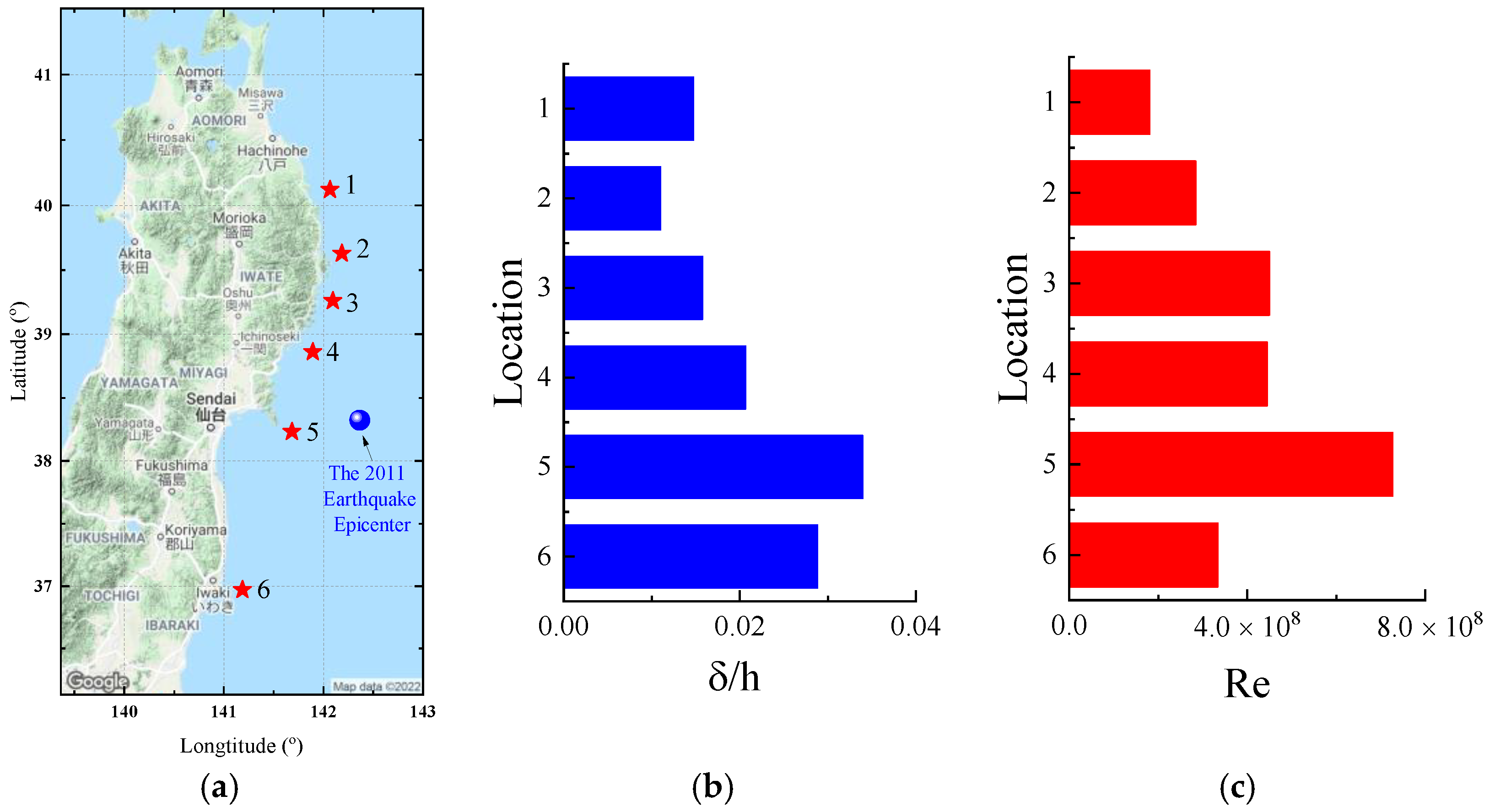
2.1. GPS Wave Gauge Data

This investigation used tsunami data [8] from six locations, as shown in Figure 1a. The result for each measuring point is illustrated using the station number shown in

Table 1. GPS wave gauge data used in this study.

No.	Measuring Station	Lattitude (deg.)	Longitude (deg.)	Water Depth (m)
1	North Iwate	40.1167	142.0667	125
2	Central Iwate	39.6272	142.1867	200
3	South Iwate	39.2586	142.0969	204
4	North Miyagi	38.8578	141.8944	160
5	Central Miyagi	38.2325	141.6836	144
6	Fukushima	36.9714	141.1856	137

. It is to be noted that Figure 1b,c is explained in detail later.

In order to investigate the tsunami-induced bottom boundary layer characteristics, the estimated tsunami-induced velocity was based directly on the measured water surface elevations at the GPS stations, as similar to [6]. The equation can be expressed as follows:

$$U(t)=\eta (t)\sqrt{\frac{g}{h}}$$

(1)

where $U(t)$ is the flow velocity, $\eta (t)$ is the water surface elevation, $h$ is the still water depth, and $g$ is the gravitational acceleration.

Figure 2 shows the flow velocity results from Equation (1) for six stations, which indicate a highly irregular waveform.

2.2. Numerical Analysis Using the k-ω Turbulence Model

The present study used the same k-ω model as in the previous study by [2,9]. For the 1-D incompressible unsteady flow, the equation of motion within the boundary layer can be expressed as follows:

$$\frac{\partial u}{\partial t}=-\frac{1}{\rho }\frac{\partial p}{\partial x}+\frac{1}{\rho }\frac{\partial \tau }{\partial z}$$

(2)

where $u$ is the horizontal velocity in the boundary layer, $t$ is the time, p is the pressure, $\rho$ is the fluid density, $\tau$ is the shear stress, x is the horizontal coordinate, and z is the vertical coordinate taken as positive upward from the bottom surface.

At the location outside of the boundary layer, the pressure gradient term is equal to the temporal variation free-stream velocity, $U(t)$, obtained from Equation (1). In addition, the shear stress for turbulence flow is calculated by introducing the eddy viscosity model. Hence, Equation (2) can be rewritten as follows:

$$\frac{\partial u}{\partial t}=-\frac{1}{\rho }\frac{\partial U}{\partial x}+\frac{1}{\rho }\frac{\partial }{\partial z}\left\{(\mathsf{\nu }+{\mathsf{\nu }}_t)\frac{\partial u}{\partial z}\right\}$$

(3)

where $\mathsf{\nu }$ is the molecular kinematic viscosity, and ${\mathsf{\nu }}_t$ is the eddy viscosity.

Although the nonlinear advection term is not considered in Equation (3), this linearized boundary layer equation has been successfully employed and validated even for nonlinear wave-induced boundary layers by imposing a pressure gradient under the nonlinear waves, such as hyperbolic wave [10], solitary wave [11,12,13], saw-tooth wave [14], and cnoidal wave [15]. In addition, the same Fortran code that was developed and validated by our group [12,15,16] was utilized in this study to ensure the reliability of the model results.

The system is closed using the standard two-equation k-ω model proposed by [17] and further developed by [18]. The transport equations for turbulent kinetic energy $k$ and the specific dissipation rate of the turbulent kinetic energy ω can be expressed as follows:

Turbulent kinetic energy ($k$):

$$\frac{\partial k}{\partial t}=\frac{\partial }{\partial z}\left\{(\mathsf{\nu }+{\mathsf{\nu }}_t{\sigma }_{k\omega })\frac{\partial k}{\partial z}\right\}+{\mathsf{\nu }}_t{(\frac{\partial u}{\partial z})}^2-{\beta }^{*}k\omega$$

(4)

Specific dissipation rate (ω):

$$\frac{\partial \omega }{\partial t}=\frac{\partial }{\partial z}\left\{(\mathsf{\nu }+{\mathsf{\nu }}_t{\sigma }_{\omega })\frac{\partial \omega }{\partial z}\right\}+\gamma {(\frac{\partial u}{\partial z})}^2-\beta {\omega }^2+2(1-F_1){\sigma }_{\omega 2}\frac{1}{\omega }\frac{\partial k}{\partial z}\frac{\partial \omega }{\partial z}$$

(5)

From k and ω, the eddy viscosity can be calculated as

$${\mathsf{\nu }}_t=\frac{k}{\omega }$$

(6)

where the values of the model constants are given as ${\sigma }_{k\omega }$ = 0.5 and ${\beta }^{*}$ = 0.09, which describes the nonlinear transition of a flow regime from a laminar flow to a turbulent flow in Menter’s model, ${\sigma }_{\omega }$ = 0.5, $\gamma$ = 0.553, and $\beta$ = 0.075 respectively, and $F_1$ is a blending function, given as:

$$F_1=\tanh ({\arg }_1^4)$$

(7)

where

$${\arg }_1=\min \left[\max (\frac{\sqrt{k}}{0.09\omega d_1},\frac{500\mathsf{\nu }}{d_1^2\omega }),\frac{4{\sigma }_{\omega 2}k}{{\mathit{CD}}_{k\omega }{d}_1^2}\right]$$

(8)

in which $d_1$ is the distance of the cell to the nearest surface, and ${\mathit{CD}}_{k\omega }$ is the positive portion of the cross-diffusion term of Equation (5) defined as:

$${\mathit{CD}}_{k\omega }=\max (2{\sigma }_{\omega 2}\frac{1}{\omega }\frac{\partial k}{\partial z}\frac{\partial \omega }{\partial z},{10}^{-20})$$

(9)

Thus, Equations (3)–(5) were solved simultaneously using the free stream velocity, $U$, angular frequency, σ, kinematics viscosity, ν and water depth, $h$. An implicit finite-difference scheme with exponentially increasing grid spacing is used to solve the governing equations, allowing for more precise numerical analysis near the bottom [2]. It is determined for a detailed velocity distribution near the bottom by making a mesh interval exponentially increase from the surface of a wall to a numerical computation using an implicit scheme finite difference method. One period is divided into 150,000 as a temporal decomposition, and the magnitude of the mesh is made to increase in the vertical direction in a geometric series towards the upper part so that about ten calculating points may be arranged in a viscous sublayer. The total number of vertical layers is 101. Because the details of the calculation methodology are explained by [16], the detailed explanations are not described here. The uniform median bed sediment is set to d = 0.3 mm, and $k_s=2d$ is the Nikuradse equivalent roughness estimation [19].

In the present study, the bottom shear stress results from the k-ω model are assumed as the true values, and other proposed methods will be compared with the k-ω model results to discuss the accuracy.

3. Results and Discussion

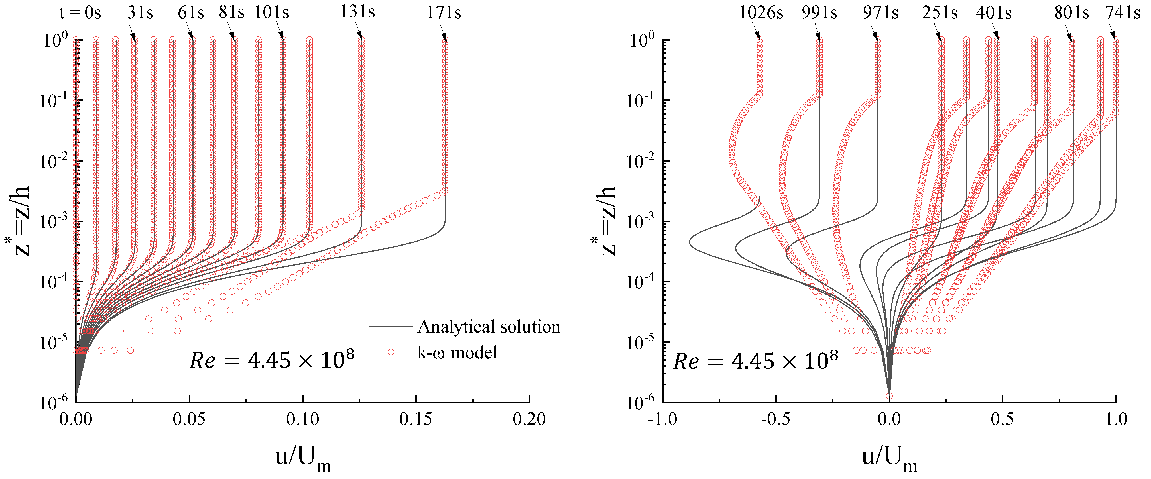
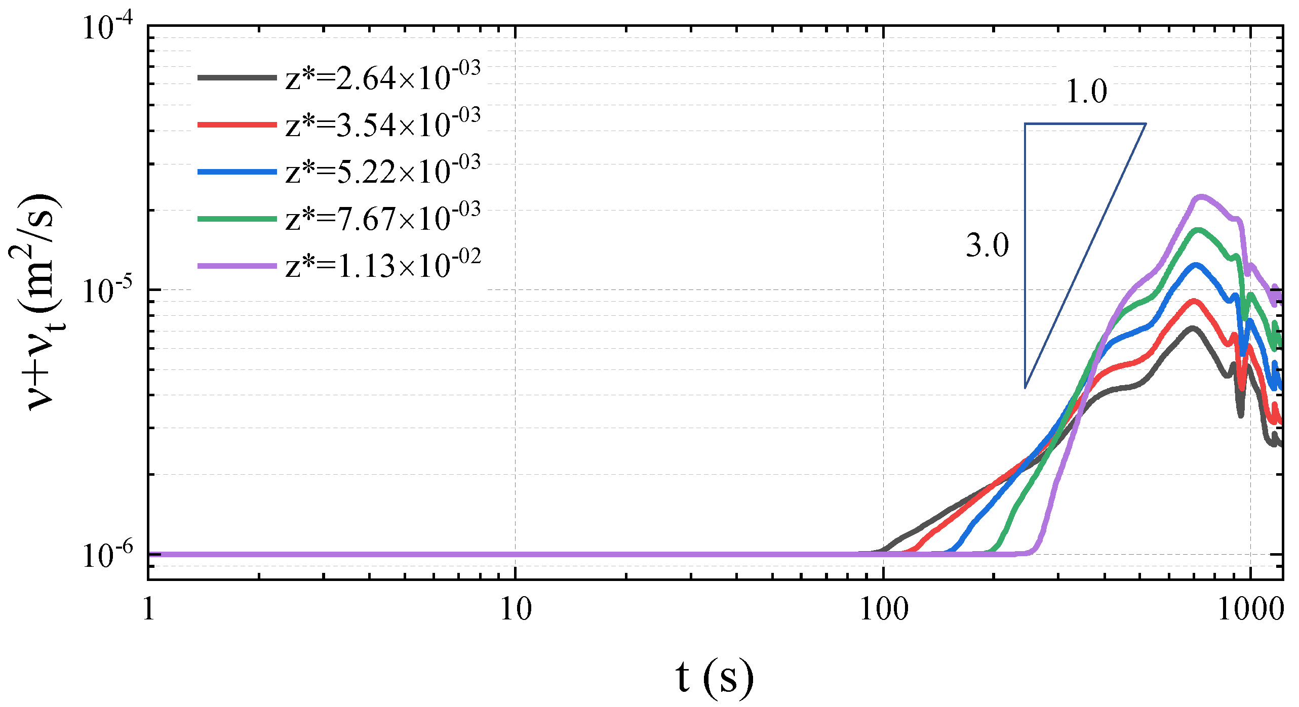
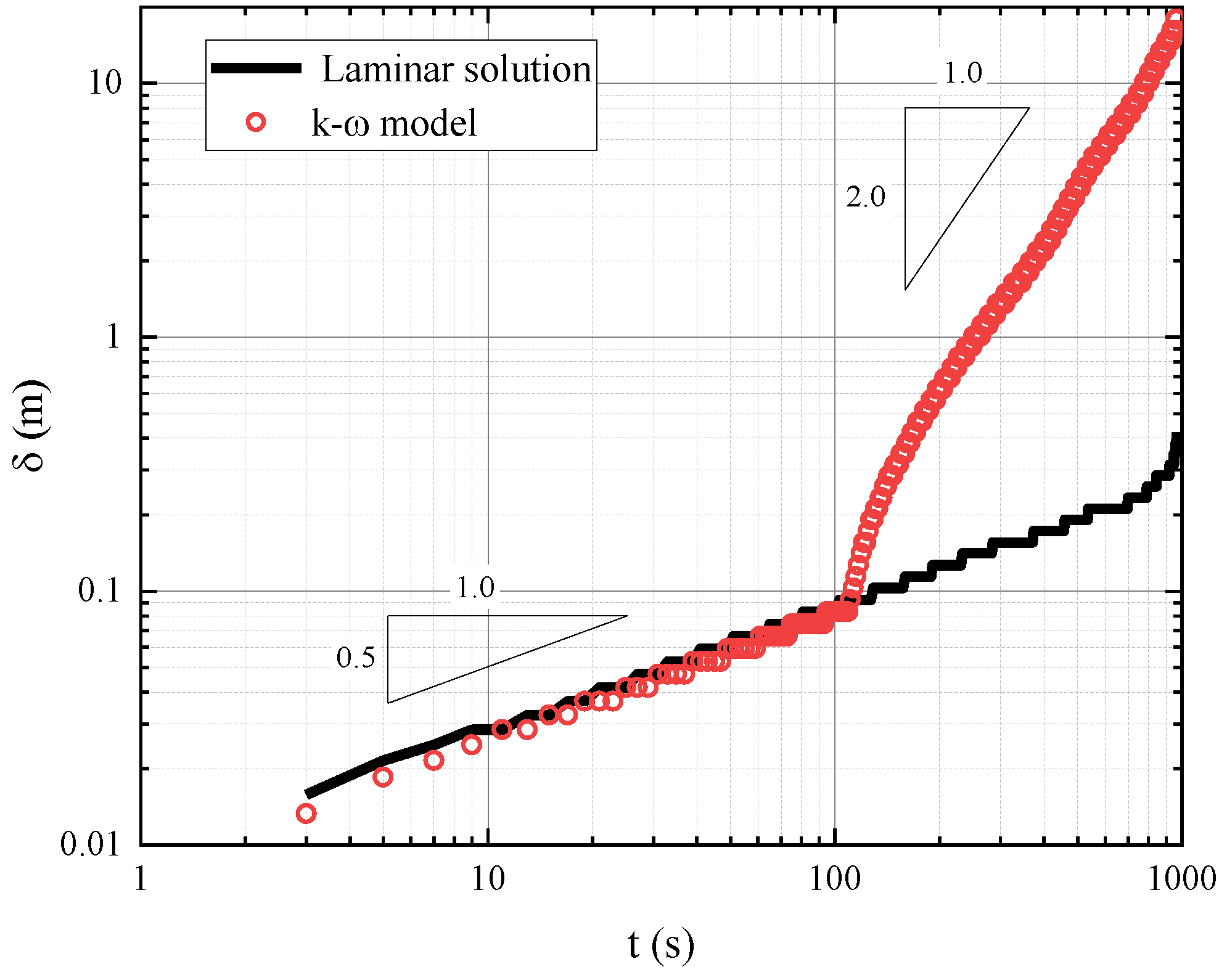
3.1. Transition from Laminar to Turbulence in the Tsunami Boundary Layer

In most of the current conventional tsunami numerical models, the tsunami wave is assumed as a longwave, and the shallow water equation can be applied. In this theory, the flow regime is classified as a turbulent flow regime, and the boundary layer thickness is developed up to the water surface. However, [6,7] found that the boundary layer near the tsunami source area is surprisingly in the laminar flow regime. Therefore, the use of the steady flow theory may not be applicable for the tsunami case. In addition, the development of a flow regime under a tsunami wave has not been studied before. In this study, the k-ω model was applied to provide detailed time variations of vertical velocity profiles.

As mentioned in [20]’s paper, Kondo [21] developed the laminar solution of the oscillating flow boundary layer under asymmetric flow velocity waveform using Laplace transformation. Although the details are omitted here, the theoretical solution is written as follows:

$$u(t,z)=U(t)-{\displaystyle \underset{0}{\overset{t}{\int }}\frac{z}{2\sqrt{\pi \mathsf{\nu }{(t-\xi )}^3}}\exp (-\frac{z^2}{4\mathsf{\nu }(t-\xi )})}U(\xi )d\xi$$

(10)

where $u(t,z)$: mainstream flow velocity, $U(t)$ is free-stream velocity, $\mathsf{\nu }$: kinematic viscosity coefficient, t: time; $\xi$ is dummy integration variable. It is possible to obtain an arbitrary flow velocity waveform by numerically integrating the above equation.

Figure 3 shows the comparison results between the k-ω model and Kondo’s analytical laminar solution under the No.4 GPS tsunami wave at selected phases. In order to quantitatively analyze the difference between the k-ω model and the analytical solution, the periodic averaged deviation, ε, which was introduced by [22], is utilized and is written as follows:

$$\epsilon ={\left[{{\displaystyle \sum _{i=1}^M\left\{\frac{U_{i(lam)}}{U_m}-\frac{U_{i(k\omega )}}{U_m}\right\}}}^2/M\right]}^{1/2}$$

(11)

where the subscripts (lam) and (kω) denote the analytical and k-ω model, respectively; $i$ is the time index in a wave; $U_m$ is the maximum velocity at the wave crest; $M=101$ is the number of vertical layers.

Figure 4 shows the time variation in the deviation difference between the k-ω model and the analytical laminar solution. The k-ω model result perfectly agrees with the laminar flow regime condition solution within 100 s of the initial stage of tsunami arrival, indicating the flow regime is laminar flow. After that, the k-ω model velocity profile tends to deviate compared to the laminar solution in the boundary layer. The flow transforms to a turbulent flow regime in an actual tsunami condition.

For determining the transition to turbulence, the spatial and temporal kinetic energy, $k$ can be computed by the k-ω model, and is shown in Figure 5. The average value of turbulent kinetic energy is normalized by the quadratic of the amplitude velocity under the crest, $U_m$. Figure 6 shows the time variation in the total molecular viscosity, $\mathsf{\nu }$, and eddy viscosity, ${\mathsf{\nu }}_t$, at several elevations near the bottom. The computed values of $k$ and total viscosity remained nearly constant until the suddenly increased transition point to turbulence around 100 s.

The transition from laminar to turbulence conditions can also be observed by analyzing the bottom boundary layer thickness development. Using the dimensional analysis for the partial derivative of Equation (2) for a steady flow, many studies have shown that the boundary layer under a laminar condition is proportional to the squared root of kinematic viscosity, $\mathsf{\nu }$, and time as $\delta =\sqrt{\mathsf{\nu }t}$. Under a turbulent flow, the thickness of a boundary layer development can be estimated as $\delta =\sqrt{{\mathsf{\nu }}_{t}t}$.

Figure 7 shows the log-plot analysis results of the bottom boundary layer thickness development from both the k-ω model and the analytical solution. Because of the absence of overshooting velocity during the accelerating phase, the bottom boundary layer thickness is consistently defined as the distance away from the bed surface where the velocity reaches 99% of the positive free-stream velocity and 101% of the negative free-stream velocity. During the first 100 s, the boundary layer thickness develops in an exponential of 1/2 with time, and thus confirms the flow is in laminar flow. The result of the boundary layer thickness by the k-ω model when transitioning to turbulent flow shows that it is very similar to the squared function of the time. Based on the above formula for turbulent boundary layer thickness, in order to obtain this quadratic relationship, the eddy viscosity ν_t should be proportional to the cubed function of the time in the turbulent flow. Figure 6 clearly suggests this relationship.

As discussed above, the velocity profile from the k-ω model result excellently agrees with the analytical laminar solution within 100 s of the initial stage of tsunami arrival, indicating the flow regime is in a laminar flow. Hence, the k-ω model velocity profile tends to deviate from the laminar solution in the boundary layer to transform to a turbulent flow regime in an actual tsunami condition. Although the transition from laminar flow to turbulence in the tsunami boundary layer exists, its duration is negligible.

3.2. Characteristics of the Turbulent Structure of Tsunami Bottom Boundary Layer Using the 2011 Tohoku Tsunami Waveform

3.2.1. Inspection of the Depth-Limitation Condition

The thickness of the wave boundary layer is calculated using the full range equation [23,24]. However, to apply this equation to non-sinusoidal waves such as the surveyed tsunami waveform, it is necessary to assume a certain equivalence.

The flow velocity waveform calculated by Equation (1) is shown in Figure 2. The maximum flow velocity at the outer edge of the wave boundary layer, $U_m$, is estimated from the first wave; and the representing length in a wave boundary layer is not the water depth, $h$, but the maximum water particle excursion length, $a_m$. In the case of sinusoidal waves, the following equation can be applied:

$$a_m=\frac{U_m}{\sigma }$$

(12)

where $\sigma$: the angular frequency. However, Equation (12) cannot be used in this investigation. Therefore, a method developed by [25] was utilized. The $a_m$ is calculated by integrating the positive flow velocity of the first wave, and $a_m$ is computed by dividing the integration by 2. The formula is written as.

$$a_m(t)=\frac{1}{2}{\displaystyle \underset{t_0}{\overset{t}{\int }}U(t)dt}$$

(13)

where $t_0$ is the time of the previous zero crossing of the free stream velocity.

Using Equation (13), the dimensionless boundary layer thickness (δ/h) can be computed, and the result is shown in Figure 1b. According to this, the ratio δ/h ranges from 0.011 to about 0.034, which means the boundary layer does not span the entire water surface for all six cases. Therefore, applying the steady friction law, such as the Manning formula, is invalid.

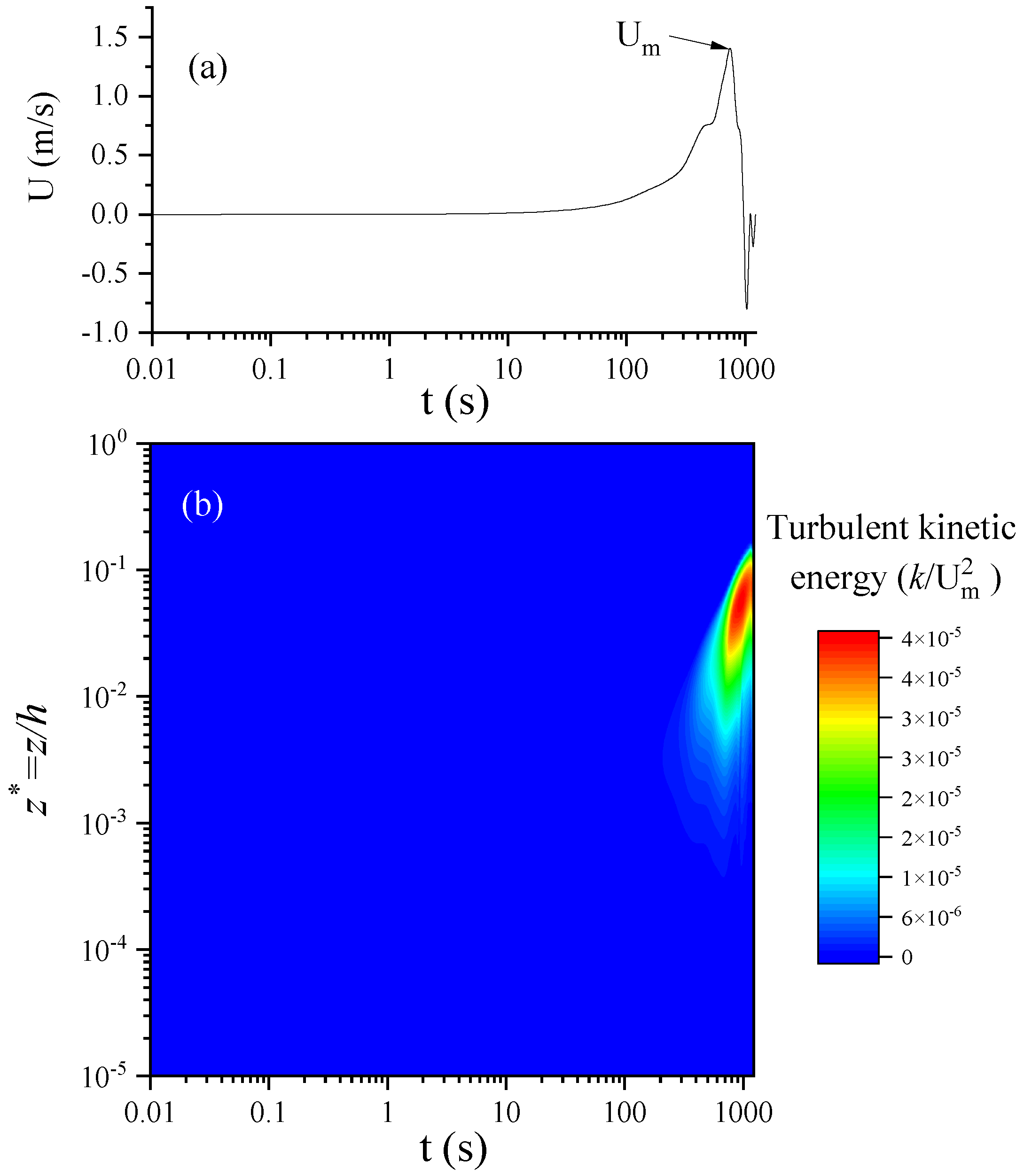
3.2.2. Inspection of the Transition to Turbulence

In this section of the study, we examined the turbulent flow transition in a wave boundary layer. According to the investigation of the hypothetical tsunami-induced flow regime of the bottom boundary layer by [7], it has been reported that a boundary layer is in a laminar flow regime near the tsunami source area. For this reason, it is crucial to clarify the location where the transition flow happened.

As previously mentioned, the relevant length in a wave boundary layer is the maximum water particle excursion length $a_m$. Therefore, the Reynolds number is calculated by the following equation:

$$R_e=\frac{U_m{a}_m}{\mathsf{\nu }}$$

(14)

The result is shown in Figure 1c. According to [26,27], it has been reported that the critical Reynolds number that changes to a turbulent flow is $Re=2.5\times {10}^5$. It was found that all cases are larger than this critical value, and the Reynolds number shown in Figure 1c is in a turbulent flow region.

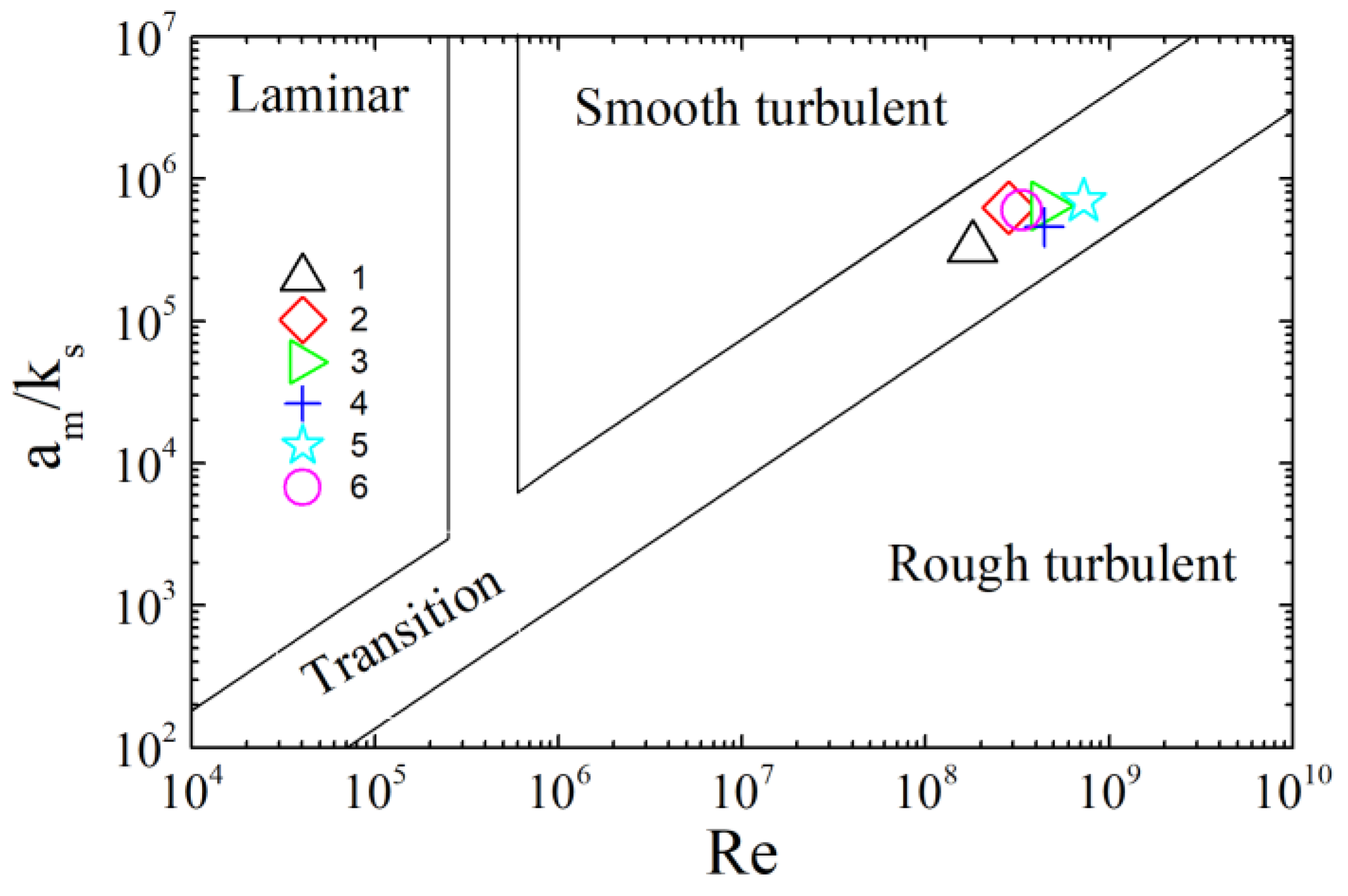
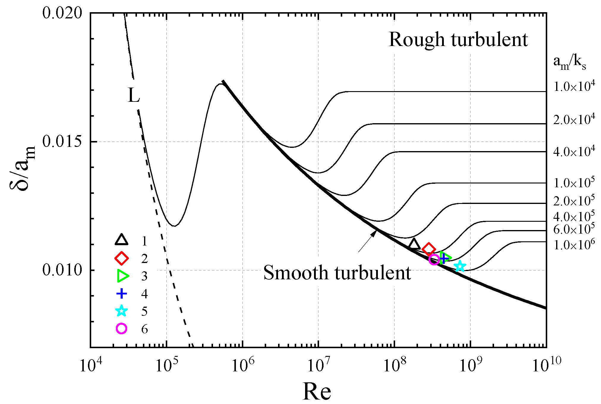
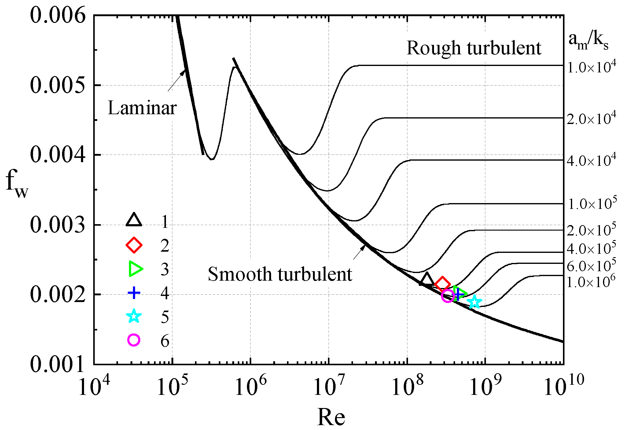
3.2.3. Inspection of the Flow Regime of the Boundary Layer

Figure 8 shows the flow regime for each measuring GPS station. Here, the flow regime classification of [23] was used. According to this, all the cases belong in the transition region from a smooth turbulent flow to a rough turbulent flow.

3.2.4. Inspection of the Transitional Characteristics of the Boundary Layer Thickness and Friction Factor

Using the full range equation of [24], the dimensionless boundary layer thickness (δ/h) and wave friction factor can be estimated and are illustrated in Figure 9 and Figure 10, respectively. It is again confirmed that all six cases are located in the turbulent transitional region from a smooth turbulent flow to a rough turbulent flow. Therefore, the judgment of the flow regime is important in the boundary layer under a tsunami. In addition, under the actual tsunamis, the friction coefficient of a transition region has a small value compared with the friction coefficient of a rough turbulent flow.

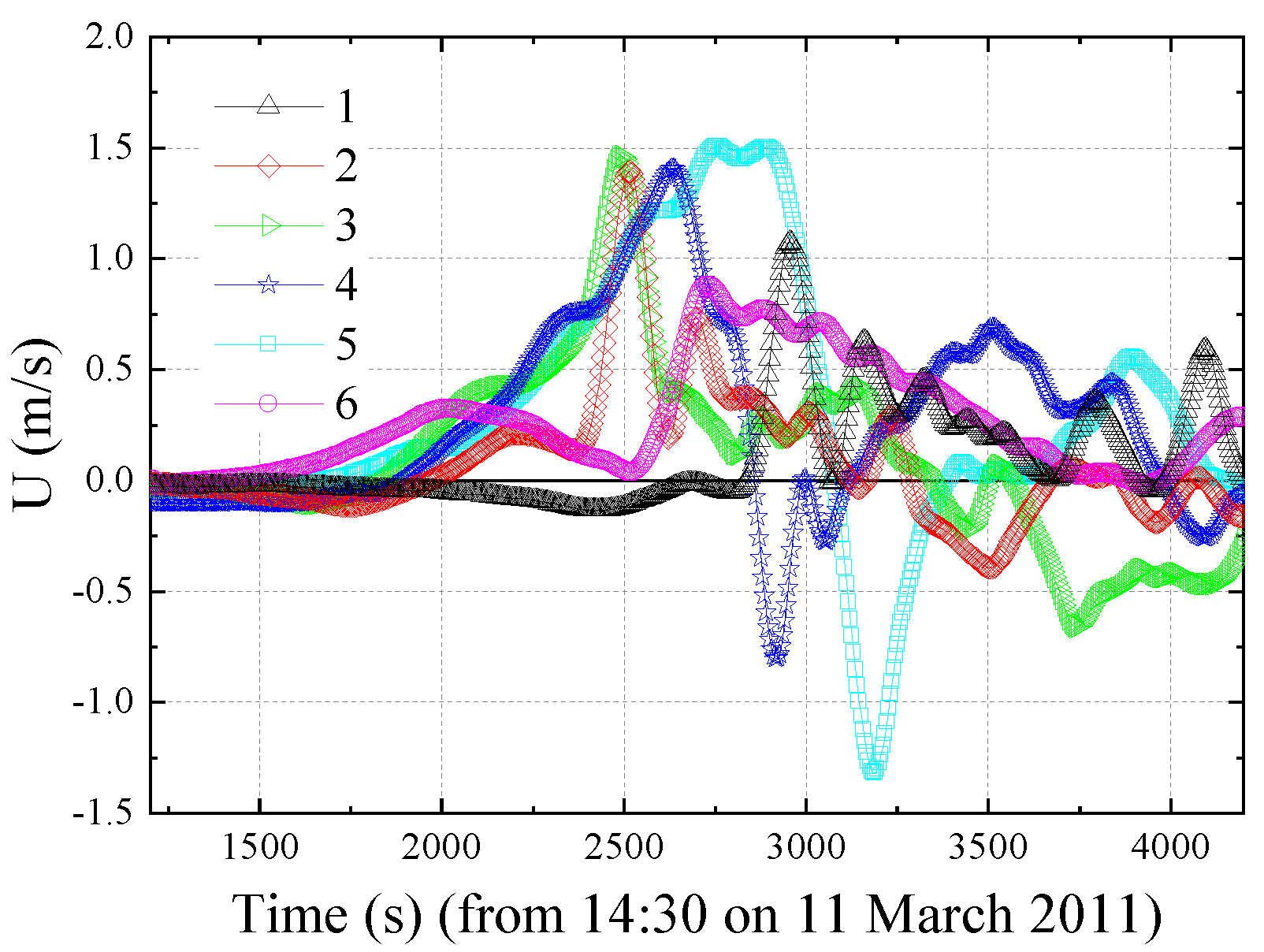
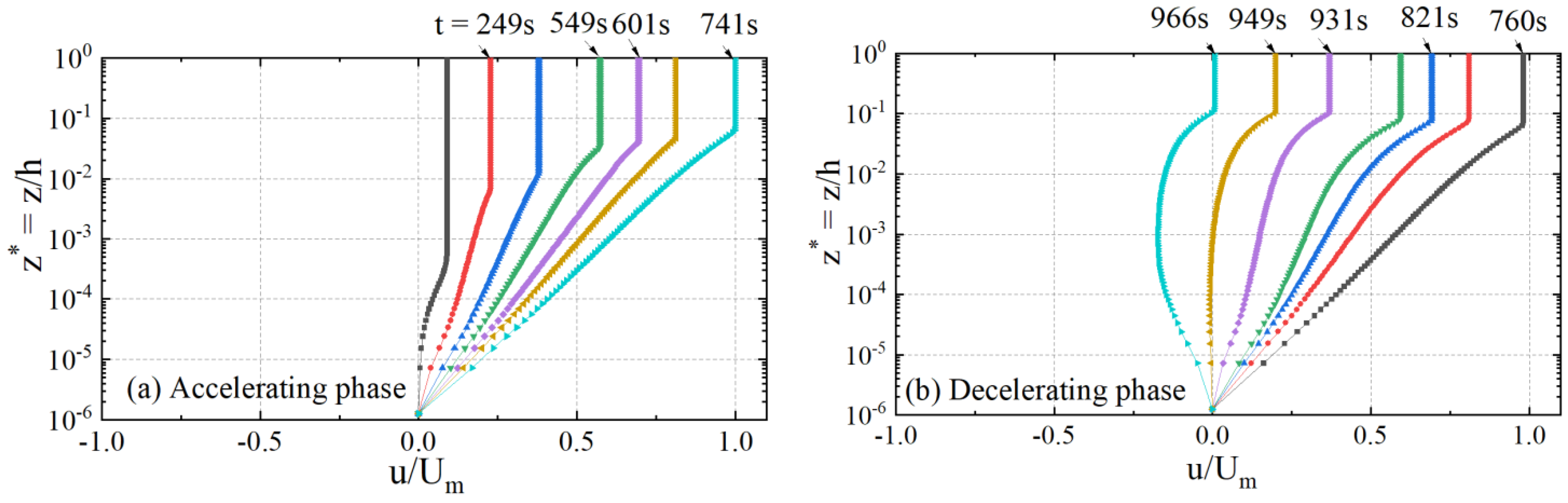
3.2.5. Tsunami-Induced Velocity

The flow velocity distribution obtained by numerical computation is shown in Figure 11. The dimensionless vertical coordinates and the flow velocity are normalized by the water depth, $h$, and the maximum flow velocity $U_m$. The acceleration phase in Figure 11a consists of a uniform flow above the boundary layer and logarithmic distribution inside the boundary layer. The development characteristic of the wave boundary layer is similar to that of an infinite flat plane. However, the velocity distribution of the acceleration phase differs significantly from the well-known periodic wave boundary layer (e.g., [28,29]). Instead, it is similar to the velocity distribution of a monotonous boundary layer.

Moreover, δ/h = 0.05, and the log-law distribution is not developed for the water surface like in an open channel and a large velocity gradient near the bottom. It is clear that the friction law of steady flows, such as the Manning formula, cannot be used.

The overshooting of velocity is remarkable at t = 966 s during the decelerating phase, as shown in Figure 11b. As mentioned above, the characteristic of the velocity distribution ranging from the acceleration phase to the decelerating phase is closely similar to the experimental result of the velocity distribution in a boundary layer under a solitary wave [30,31].

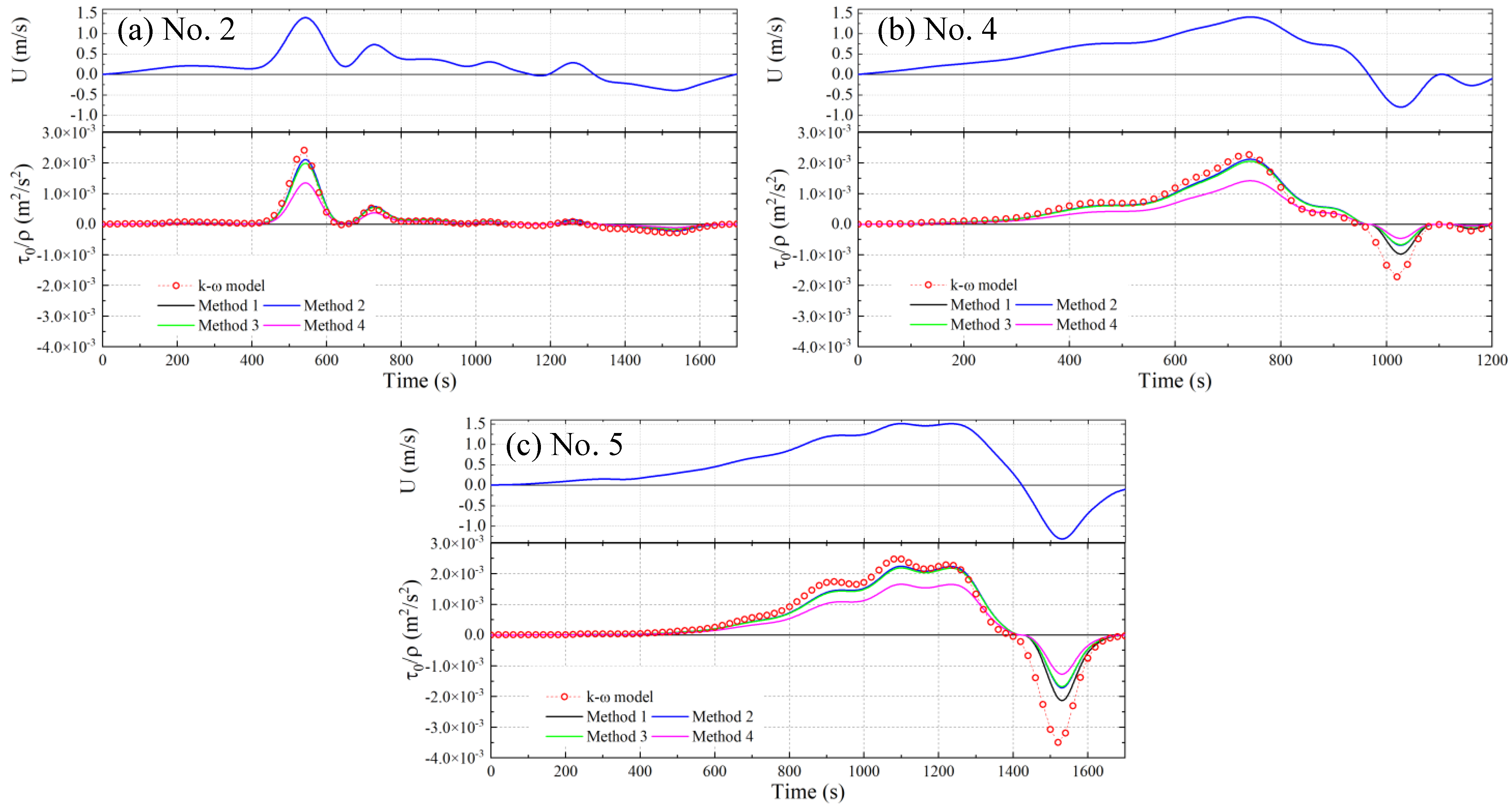
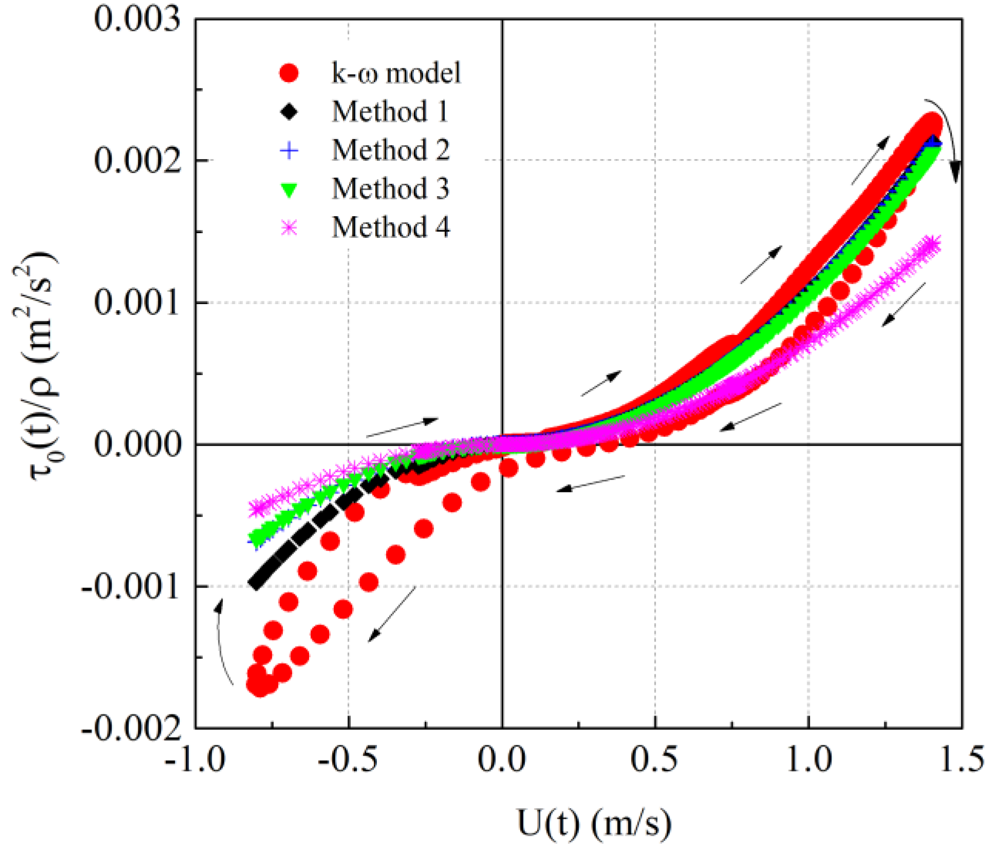
3.2.6. Tsunami-Induced Bottom Shear Stress

Figure 12 shows the time variation in the bottom shear stress obtained using the k-ω model at three measuring stations (No.2, No.4, and No.5) among the six stations in Table 1. The methods used in the figures are discussed in a later section. From t = 0 s to t = 520 s, the increase in shear stress is more rapid than the flow velocity.

Figure 13 shows the relationship between the instantaneous bottom shear stress ${\tau }_0\left(t\right)$ and the boundary layer outer edge flow velocity $U\left(t\right)$. The result confirms that the shear stress is proportional to the squared flow velocity. Therefore, a loop-like relationship is observed, as shown in Figure 13. However, the conventional expression for accurately estimating the bottom shear stress is required for practical application instead of the k-ω model. Therefore, we propose several simple methods in the next section.

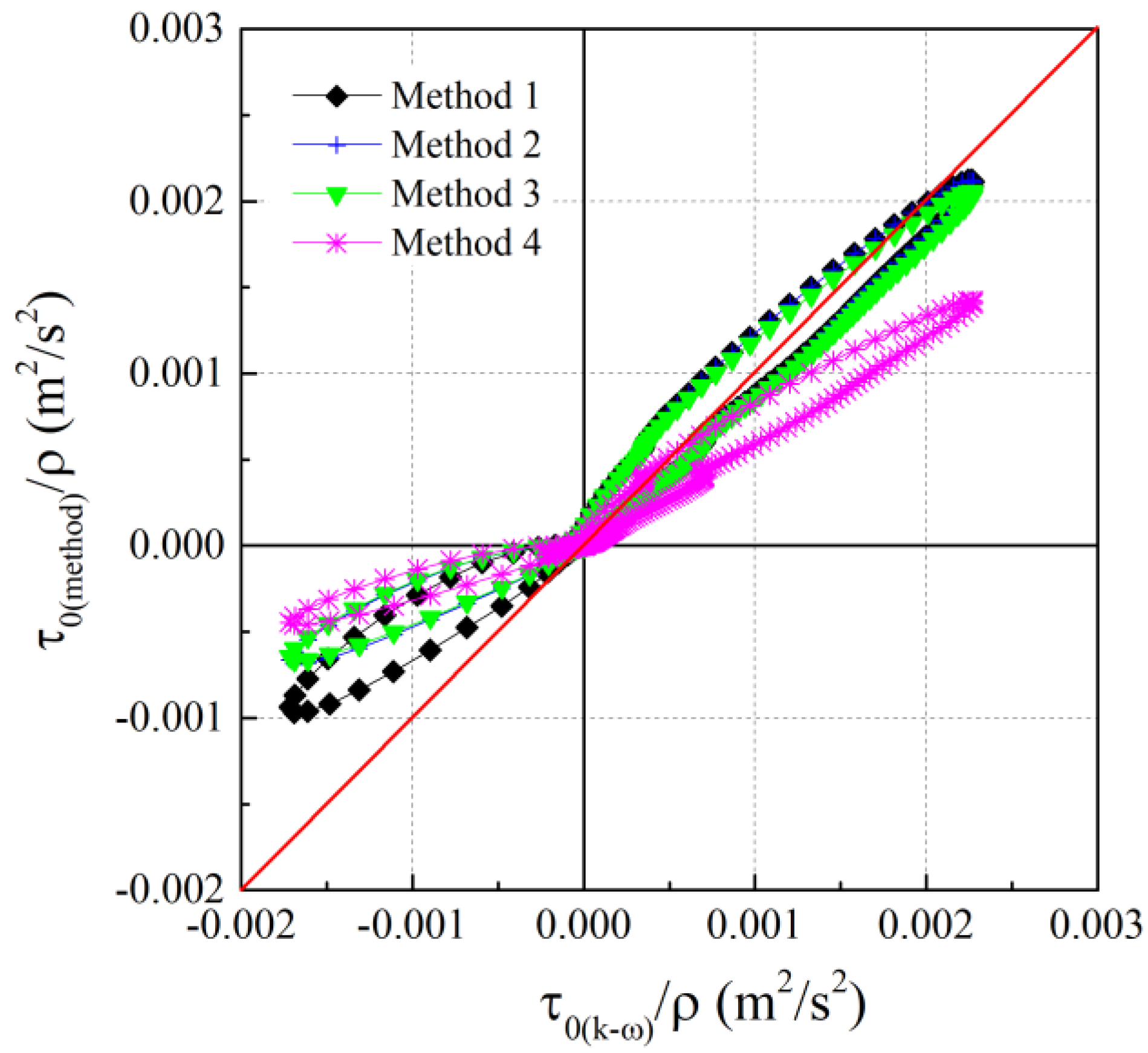
4. Simple Methods of Calculating Bottom Shear Stress

As discussed in previous sections, the tsunami-induced bottom shear stress needs to be calculated using the wave friction theory instead of the steady friction theory. However, all wave friction theories [11,12,13,14,15,16] are developed based on simple waveforms such as sinusoidal, solitary, and cnoidal waves, and a few are based on an irregular wave [23,32,33]. Therefore, we intended to develop simple methods to apply the wave friction factor, such as the full range equation by Tanaka and Thu (1994), in practice without using a complex model such as the k-ω model. One of the difficulties is how to determine the value of $a_m$. In this study, three methods are proposed to calculate $a_m$, as shown in

Table 2. Calculation method of bottom shear stress.

Method	Explanation
k-ω model (truth)	Numerical solution using the turbulence model.
Method 1	Using $a_{m1}$$, a_{m2}$, … for each crest phase and trough phase from numerical integration of the velocity, calculate $f_{w1}$$, f_{w2}$, … for each.
Method 2	Using $a_{m1}$ from the first positive wave, calculate $f_{w1}$, and use this single value for subsequent waves.
Method 3	Using the $U_m$ and $T_1$ (duration of the first positive wave), calculate $a_{m1}=U_m{T}_1/2\pi$ to obtain $f_{w1}$, and use this single value for subsequent waves.
Method 4	Steady flow friction coefficient $f_c$ (from log law).

. Method 1 uses Equation (13) for each wave crest phase and wave trough phase, then uses $a_{m1}$, $a_{m2}$, … to calculate $f_{w1}$, $f_{w2}$, … for each phase. Method 2 applies Equation (13) for the first maximum positive velocity phase to obtain $a_{m1}$ and f_w1, then assigns these values to the subsequent phases. Method 3 calculates $a_{m1}$ and f_w1 based on the sinusoidal wave formula for the first wave, and these values are applied to the subsequent phases. Method 4 uses the conventional steady flow friction f_c theory.

Finally, the bottom shear stress results from the k-ω model are assumed to be the true values in the present study, and other proposed methods are compared with the k-ω model results to discuss the accuracy.

Figure 12 and Figure 14 compare these four methods’ tsunami-induced bottom shear stress results with the k-ω model. As can be seen, Methods 1, 2, and 3 give good results in the first positive wave phase. However, they are underestimated compared to the k-ω model results in the subsequent negative wave phase. Nonetheless, Method 1 still provides better comparison results. Method 4 always gives remarkably underestimated results compared to the k-ω model in all phases.

For a more quantitative assessment of the methods’ accuracy, the root mean squared error (RMSE) was calculated for the trough and crest flow velocity phases, as shown in Figure 15. The underestimation in the subsequent trough flow velocity phase is more remarkable even with the wave friction coefficient methods. The significant difference is due to the limitation of the computation method that uses the knowledge of the sinusoidal waves. Therefore, further investigation is needed to consider the wave-like characteristics of such non-sinusoidal waveforms.

5. Conclusions

The characteristics of the bottom boundary layer under a tsunami were examined based on the surveyed tsunami waveform. Due to the irregularity of the tsunami waveform, the bottom shear stress could not be estimated accurately using the knowledge of sinusoidal waves. In this study, we proposed simple methods for calculating bottom shear stress for a tsunami with irregular waveforms. The new methods are comparable with the k-ω model results. In the future, the effect of the history of the reflecting waveform shape should be considered in order to increase the accuracy of the tsunami-induced bottom shear stress estimation.

References

1. Jonsson, I.G. Wave boundary layer and friction factors. Coast. Eng. Proc. 1966, 1, 127–148. [Google Scholar]
2. Tinh, N.X.; Tanaka, H. Study on boundary layer development and bottom shear stress beneath a tsunami. Coast. Eng. J. 2019, 61, 574–589. [Google Scholar] [CrossRef]
3. Tanaka, H.; Tinh, N.X.; Yu, X.; Liu, G. Development of depth-limited wave boundary layers over a smooth bottom. J. Mar. Sci. Eng. 2021, 9, 27. [Google Scholar] [CrossRef]
4. Lacy, J.R.; Rubin, D.M.; Buscombe, D. Currents, drag, and sediment transport induced by a tsunami. J. Geophys. Res. 2012, 117, C9. [Google Scholar] [CrossRef]
5. Makris, A.; Lacy, J.R.; Fuhrman, D.R. Numerical Simulation of the Boundary Layer Flow Generated in Monterey Bay, California, by the 2010 Chilean Tsunami Case Study. J. Waterw. Port Coast. Ocean. Eng. 2021, 147, 6. [Google Scholar] [CrossRef]
6. Williams, I.A.; Fuhrman, D.R. Numerical simulation of tsunami-scale wave boundary layers. Coast. Eng. 2016, 110, 17–31. [Google Scholar] [CrossRef] [Green Version]
7. Tanaka, H.; Tinh, N.X.; Sana, A. Transitional behavior of a flow regime in shoaling tsunami boundary layers. J. Mar. Sci. Eng. 2020, 8, 700. [Google Scholar] [CrossRef]
8. Kawai, H.; Satoh, M.; Kawaguchi, K.; Seki, K. Characteristics of the 2011 Tohoku tsunami waveform acquired around Japan by Nowphas equipment. Coast. Eng. J. 2013, 55, 1350008. [Google Scholar] [CrossRef]
9. Tinh, N.X.; Tanaka, H.; Yu, X.; Liu, G. Numerical implementation of wave friction factor into the 1D tsunami shallow water equation model. Coast. Eng. J. 2021, 63, 174–186. [Google Scholar] [CrossRef]
10. Larson, M. A closed form solution for turbulent wave boundary layers. Coast. Eng. Proc. 1996, 1, 3244–3256. [Google Scholar]
11. Liu, P.L.-F.; Park, Y.S.; Cowen, E.A. Boundary layer flow and bed shear stress under a solitary wave. J. Fluid Mech. 2007, 574, 449–463. [Google Scholar] [CrossRef]
12. Suntoyo; Tanaka, H. Numerical modeling of boundary layer flows for a solitary wave. J. Hydro-Environ. Res. 2009, 3, 129–137. [Google Scholar]
13. Vittori, G.; Blondeaux, P. The boundary layer at the bottom of a solitary wave and implications for sediment transport. Prog. Oceanogr. 2014, 120, 399–409. [Google Scholar] [CrossRef]
14. Suntoyo; Tanaka, H.; Sana, A. Characteristics of turbulent boundary layers over a rough bed under saw-tooth waves and its application to sediment transport. Coast. Eng. 2008, 55, 1102–1112. [Google Scholar] [CrossRef]
15. Suntoyo; Tanaka, H. Effect of bed roughness on turbulent boundary layer and net sediment transport under asymmetric waves. Coast. Eng. 2009, 56–59, 960–969. [Google Scholar]
16. Sana, A.; Ghumman, A.R.; Tanaka, H. Modeling of a rough-wall oscillatory boundary layer using two-equation turbulence models. J. Hydraul. Eng. 2009, 135, 60–65. [Google Scholar] [CrossRef]
17. Wilcox, D.C. Reassessment of the scale determining equation for advanced turbulence models. AIAA J. 1988, 26, 1299–1310. [Google Scholar] [CrossRef]
18. Menter, F.R. Two-equation eddy-viscosity turbulence models for Eng. applications. AIAA J. 1994, 32, 1598–1605. [Google Scholar] [CrossRef] [Green Version]
19. Kamphuis, J.W. Determination of sand roughness for fixed bed. J. Hydraul. Res. 1974, 12, 193–203. [Google Scholar] [CrossRef]
20. Nadaoka, K.; Yagi, H.; Nihei, Y.; Nomoto, K. Characteristics of turbulent structure in asymmetrical oscillatory flow. Proc. Coast. Eng. JSCE 1994, 41, 141–145. (In Japanese) [Google Scholar]
21. Kondo, J. Operational Calculus; Baifukan: Tokyo, Japan, 1956. (In Japanese) [Google Scholar]
22. Tanaka, H.; Sumer, B.M.; Lodahl, C. Theoretical and experimental investigation on laminar boundary layers under cnoidal wave motion. Coast. Eng. Japan 1998, 40, 81–89. [Google Scholar] [CrossRef]
23. Tanaka, H.; Thu, A. Full-range equation of friction coefficient and phase difference in a wave-current boundary layer. Coast. Eng. 1994, 22, 237–254. [Google Scholar] [CrossRef]
24. Tanaka, H.; Tinh, N.X.; Sana, A. Improvement of the full-range equation for wave boundary layer thickness. J. Mar. Sci. Eng. 2020, 8, 573. [Google Scholar] [CrossRef]
25. Larsen, B.E.; Fuhrman, D.R. Full-scale CFD simulation of tsunamis. Part 2 Boundary layers and bed shear stresses. Coast. Eng. 2019, 151, 42–57. [Google Scholar] [CrossRef]
26. Tanaka, H.; Shuto, N. Friction laws and flow regimes under wave and current motion. J. Hydraul. Res. 1984, 22, 245–261. [Google Scholar] [CrossRef]
27. Tanaka, H.; Sana, A. Numerical study on transition to turbulence in a wave boundary layer. The EUROMECH 310 Proc. In Sediment Transport Mechanisms in Coastal Environments and Rivers; World Scientific: Singapore, 1994; pp. 14–25. [Google Scholar]
28. Jensen, B.L.; Sumer, B.M.; Fredsøe, J. Turbulent oscillatory boundary layers at high Reynolds numbers. J. Fluid Mech. 1989, 206, 265–297. [Google Scholar] [CrossRef] [Green Version]
29. Tanaka, H.; Chian, S.C.; Shuto, N. Experiments on an oscillatory flow accompanied with a unidirectional motion. Coast. Eng. Japan 1983, 26, 19–37. [Google Scholar] [CrossRef]
30. Sumer, B.M.; Jensen, P.M.; Sørensen, L.B.; Fredsøe, J.; Liu, P.L.-F.; Cartesen, S. Coherent structures in wave boundary layers. Part 2. Solitary motion. J. Fluid Mech. 2010, 646, 207–231. [Google Scholar] [CrossRef]
31. Tanaka, H.; Winarta, B.; Suntoyo; Yamaji, H. Validation of a new generation system for bottom boundary layer beneath solitary wave. Coast. Eng. 2012, 59, 46–56. [Google Scholar] [CrossRef]
32. Yuan, J. Turbulent boundary layers under irregular waves and currents Experiments and the equivalent-wave concept. J. Geophys. Res. Oceans 2016, 121, 2616–2640. [Google Scholar] [CrossRef]
33. Tanaka, H.; Samad, M.A. Prediction of instantaneous bottom shear stress for turbulent plane bed condition under irregular waves. J. Hydraul. Res. 2006, 44, 94–106. [Google Scholar] [CrossRef]
Figure 1. (a) Location of the GPS station, (b) boundary layer thickness, (c) Reynolds number.
Jmse 10 00173 g001
Figure 2. The estimated tsunami-induced flow velocity from the measured water surface elevation.
Jmse 10 00173 g002
Figure 3. Comparison of the velocity profile for the case No. 4 between the k-ω model and the analytical laminar solution.
Jmse 10 00173 g003
Figure 4. Time variation in the deviation difference between the k-ω model and the analytical laminar solution results.
Jmse 10 00173 g004
Figure 5. (a) Time variation in free stream velocity, (b) distribution of turbulent kinetic energy.
Jmse 10 00173 g005
Figure 6. Time variation of the total molecular viscosity and eddy viscosity at several elevations near the bottom.
Jmse 10 00173 g006
Figure 7. Transitional behavior from laminar flow regime to turbulent flow regime.
Jmse 10 00173 g007
Figure 8. Flow regime of the 2011 tsunami.
Jmse 10 00173 g008
Figure 9. Bottom boundary layer thickness.
Jmse 10 00173 g009
Figure 10. Wave friction coefficient.
Jmse 10 00173 g010
Figure 11. Flow velocity distribution under the observed tsunami at the GPS No.4 during (a) the accelerating phase and (b) the decelerating phase.
Jmse 10 00173 g011
Figure 12. Flow velocity and bottom shear stress at the measuring point (a) No. 2, (b) No. 4, and (c) No. 5.
Jmse 10 00173 g012
Figure 13. Relationship between τ 0 ( t ) / ρ and U ( t ) .
Jmse 10 00173 g013
Figure 14. Comparison of other methods with the k-ω model results.
Jmse 10 00173 g014
Figure 15. RMSE of each calculation method.
Jmse 10 00173 g015