


Social Structure and Temporal Distribution of Tursiops truncatus in the Gulf of Taranto (Central Mediterranean Sea)

 , , ,
, , ,  and
and 
Abstract
1. Introduction
2. Materials and Methods
2.1. Study Area
2.2. Data Collection
2.3. Data Analysis
2.3.1. Photo-Identification Process
2.3.2. Site Fidelity
- The monthly sighting rate (MR), defined as the number of months a dolphin was identified as a proportion of the total number of months in which at least one survey was conducted;
- The yearly sighting rate (YR), defined as the number of calendar years a dolphin was identified as a proportion of the total surveyed;
- The seasonal sighting rates (SR), defined as the number of seasons a dolphin was identified as a proportion of the total number of seasons surveyed;
- The relative span-time (RST), defined as the portion of the whole observation time elapsed between the first and last ‘captures’ of the individual.
2.3.3. Residency Pattern
2.3.4. Association Pattern and Social Structure
3. Results
3.1. Data Collection
3.2. Photo-Identification
3.3. Site Fidelity
3.4. Residency Pattern
3.5. Association Pattern and Social Structure
4. Discussion
5. Conclusions
Author Contributions
Funding
Institutional Review Board Statement
Informed Consent Statement
Data Availability Statement
Acknowledgments
Conflicts of Interest
Appendix A
References
- Alexander, R.D. The evolution of social behavior. Annu. Rev. Ecol. Evol. Syst. 1974, 5, 325–383. [Google Scholar] [CrossRef]
- Stamps, J.; Groothuis, T.G.G. The development of animal personality: Relevance, concepts and perspectives. Biol. Rev. 2010, 85, 301–325. [Google Scholar] [CrossRef] [PubMed]
- Kappeler, P.M.; van Schaik, C.P. Evolution of primate social systems. Int. J. Primatol. 2002, 23, 707–740. [Google Scholar] [CrossRef]
- Gero, S. Fundamentals of Sperm Whale Societies, Care for Calves. Master’s Thesis, Dalhousie University, Halifax, NS, Canada, 2006. [Google Scholar]
- Krützen, M.; Sherwin, W.B.; Connor, R.C.; Barré, L.M.; Van de Casteele, T.; Mann, J.; Brooks, R. Contrasting relatedness patterns in bottlenose dolphins (Tursiops sp.) with different alliance strategies. Proc. Royal Soc. B 2003, 270, 497–502. [Google Scholar] [CrossRef]
- Corner, L.A.L.; Pfeiffer, D.U.; Morris, R.S. Social-network analysis of Mycobacterium bovis transmission among captive brushtail possums (Trichosurus vulpecula). Prev. Vet. Med. 2003, 59, 147–167. [Google Scholar] [CrossRef]
- McComb, K.; Reby, D.; Baker, L.; Moss, C.; Sayialel, S. Long-distance communication of acoustic cues to social identity in African elephants. Anim. Behav. 2003, 65, 317–329. [Google Scholar] [CrossRef]
- Whitehead, H.; Richerson, P.J. The evolution of conformist social learning can cause population collapse in realistically variable environments. Evol. Hum. Behav. 2009, 30, 261–273. [Google Scholar] [CrossRef]
- Lusseau, D.; Newman, M.E. Identifying the role that animals play in their social networks. Proc. R. Soc. B 2004, 271 (Suppl. 6), S477–S481. [Google Scholar] [CrossRef] [PubMed]
- Lusseau, D.; Wilson, B.E.N.; Hammond, P.S.; Grellier, K.; Durban, J.W.; Parsons, K.M.; Barton, T.R.; Thompson, P.M. Quantifying the influence of sociality on population structure in bottlenose dolphins. J. Anim. Ecol. 2006, 75, 14–24. [Google Scholar] [CrossRef]
- Vucetich, J.A.; Peterson, R.O.; Waite, T.A. Raven scavenging favours group foraging in wolves. Anim. Behav. 2004, 67, 1117–1126. [Google Scholar] [CrossRef]
- Papale, E.; Ceraulo, M.; Giardino, G.; Buffa, G.; Filiciotto, F.; Grammauta, R.; Maccarone, V.; Mazzola, S.; Buscaino, G. Association patterns and population dynamics of bottlenose dolphins in the Strait of Sicily (Central Mediterranean Sea): Implication for management. Popul. Ecol. 2017, 59, 55–64. [Google Scholar] [CrossRef]
- Wade, P.R.; Reeves, R.R.; Mesnick, S.L. Social and behavioural factors in cetacean responses to overexploitation: Are Odontocetes less “resilient” than mysticetes? J. Mar. Sci. 2012, 2012, 567276. [Google Scholar] [CrossRef]
- Snijders, L.; Blumstein, D.T.; Stanley, C.R.; Franks, D.W. Animal social network theory can help wildlife conservation. Trends Ecol. Evol. 2017, 32, 567–577. [Google Scholar] [CrossRef] [PubMed]
- Weiss, M.N.; Ellis, S.; Croft, D.P. Diversity and Consequences of Social Network Structure in Toothed Whales. Front. Mar. Sci. 2021, 8, 688842. [Google Scholar] [CrossRef]
- Whitehead, H. Analyzing Animal Societies: Quantitative Methods for Vertebrate Social Analysis; University of Chicago Press: Chicago, IL, USA, 2008. [Google Scholar]
- Burnham, K.P.; Anderson, D.R. Model Selection and Inference: A Practical Information-Theoretic Approach, 2nd ed.; Springer: New York, NY, USA, 2002. [Google Scholar] [CrossRef]
- Whitehead, H. SOCPROG programs: Analysing animal social structures. Behav. Ecol. Sociobiol. 2009, 63, 765–778. [Google Scholar] [CrossRef]
- Cairns, S.J.; Schwager, S.J. A comparison of association indices. Anim. Behav. 1987, 35, 1454–1469. [Google Scholar] [CrossRef]
- Newman, M.E.J. Analysis of weighted networks. Phys. Rev. 2004, 70, 056131. [Google Scholar] [CrossRef]
- Whitehead, H.; Bejder, L.; Ottensmeyer, C.A. Testing association patterns: Issues arising and extensions. Anim. Behav. 2005, 69, e1–e6. [Google Scholar] [CrossRef]
- Whitehead, H.; Dufault, S. Techniques for analyzing vertebrate social structure using identified individuals. Adv. Stud. Behav. 1999, 28, 33–74. [Google Scholar]
- Whitehead, H.; James, R. Generalized affiliation indices extract affiliations from social network data. Methods Ecol. Evol. 2015, 6, 836–844. [Google Scholar] [CrossRef]
- Hohmann, G.; Fruth, B. Dynamics in social organization of bonobos (Pan paniscus). In Behavioural Diversity in Chimpanzees and Bonobos; Boesch, C., Hohmann, G., Marchant, L.F., Eds.; Cambridge University Press: Cambridge, UK, 2002; pp. 138–150. [Google Scholar]
- Mitani, J.C.; Watts, D.P.; Pepper, J.W.; Merriwether, D.A. Demographic and social constraints on male chimpanzee behaviour. Anim. Behav. 2002, 64, 727–737. [Google Scholar] [CrossRef][Green Version]
- Vonhof, M.J.; Whitehead, H.; Fenton, M.B. Analysis of Spix’s diskwinged bat association patterns and roosting home ranges reveal a novel social structure among bats. Anim. Behav. 2004, 68, 507–521. [Google Scholar] [CrossRef]
- Carter, K.D.; Seddon, J.M.; Frère, C.H.; Carter, J.K.; Goldizen, A.W. Fission-fusion dynamics in wild giraffes may be driven by kinship, spatial overlap and individual social preferences. Anim. Behav. 2013, 85, 385–394. [Google Scholar] [CrossRef]
- Fishlock, V.; Lee, P.C. Forest elephants: Fission-fusion and social arenas. Anim. Behav. 2013, 85, 357–363. [Google Scholar] [CrossRef]
- Danaher-Garcia, N.A.; Melillo-Sweeting, K.; Dudzinski, K.M. Social structure of Atlantic spotted dolphins (Stenella frontalis) off Bimini, The Bahamas (2003–2016): Alternate reasons for preferential association in delphinids. Acta Ethol. 2020, 23, 9–21. [Google Scholar] [CrossRef]
- Wang, X.; Wu, F.; Turvey, S.T.; Rosso, M.; Tao, C.; Ding, X.; Zhu, Q. Social organization and distribution patterns inform conservation management of a threatened Indo-Pacific humpback dolphin population. J. Mammal. 2015, 96, 964–971. [Google Scholar] [CrossRef]
- Hartman, K.L.; Visser, F.; Hendriks, A.J.E. Social structure of Risso’s dolphins (Grampus griseus) at the Azores: A stratified community based on highly associated social units. Can. J. Zool. 2008, 86, 294–306. [Google Scholar] [CrossRef]
- Hinde, R.A. Interactions, relationships and social structure. Man 1976, 11, 1–17. [Google Scholar] [CrossRef]
- Whitehead, H. Analysing animal social structure. Anim. Behav. 1997, 53, 1053–1067. [Google Scholar] [CrossRef]
- Pepper, J.W.; Mitani, J.C.; Watts, D.P. General gregariousness and specific social preferences among wild chimpanzees. Int. J. Primatol. 1999, 20, 613. [Google Scholar] [CrossRef]
- Croft, D.P.; James, R.; Krause, J. Exploring Animal Social Networks; Princeton University Press: Princeton, NJ, USA, 2007. [Google Scholar]
- Wey, T.; Blumstein, D.T.; Shen, W.; Jordan, F. Social network analysis of animal behaviour: A promising tool for the study of sociality. Anim. Behav. 2008, 75, 333–344. [Google Scholar] [CrossRef]
- Leatherwood, S.; Reeves, R.R. The Bottlenose Dolphin, 1st ed.; Academic. Press: San Diego, CA, USA, 1990. [Google Scholar]
- Wells, R.S.; Scott, M.D. Bottlenose dolphin Tursiops truncatus (Montagu, 1821). In Handbook of Marine Mammals, Volume VI, The Second Book of Dolphins and Porpoises; Ridgway, S.H., Harrison, R., Eds.; Academic. Press: San Diego, CA, USA, 1999; pp. 137–182. [Google Scholar]
- Reynolds, J.E.; Wells, R.S.; Eide, S.D. The Bottlenose Dolphin: Biology and Conservation; University Press of Florida: Gainesville, FL, USA, 2000. [Google Scholar]
- Bearzi, G.; Fortuna, C.M.; Reeves, R.R. Ecology and conservation of common bottlenose dolphins Tursiops truncatus in the Mediterranean Sea. Mammal Rev. 2008, 39, 92–123. [Google Scholar] [CrossRef]
- Gnone, G.; Bellingeri, M.; Dhermain, F.; Dupraz, F.; Nuti, S.; Bedocchi, D.; Moulins, A.; Rosso, M.; Alessi, J.; Mccrea, R.S.; et al. Distribution, abundance, and movements of the Bottlenose dolphin (Tursiops truncatus) in the Pelagos Sanctuary MPA (north-west Mediterranean Sea). Aquat. Conserv. Mar. Freshw. Ecosyst. 2011, 21, 372–388. [Google Scholar] [CrossRef]
- Cañadas, A.; Sagarminaga, R.; García-Tiscar, S. Cetacean distribution related with depth and slope in the Mediterranean waters off southern Spain. Deep Sea Res. I 2002, 49, 2053–2073. [Google Scholar] [CrossRef]
- Forcada, J.; Gazo, M.; Aguilar, A.; Gonzalvo, J.; Fernandez-Contreras, M. Bottlenose dolphin abundance in the NW Mediterranean: Addressing heterogeneity in distribution. Mar. Ecol. Prog. Ser. 2004, 275, 275–287. [Google Scholar] [CrossRef]
- Santacesaria, F.C.; Bellomo, S.; Fanizza, C.; Maglietta, R.; Renò, V.; Cipriano, G.; Carlucci, R. Long-term residency of Tursiops truncatus in the Gulf of Taranto (Northern Ionian Sea, Central-eastern Mediterranean Sea). In Proceedings of the IMEKO Metrology for the Sea, Genova, Italy, 3–5 October 2019. [Google Scholar]
- Coll, M.; Piroddi, C.; Albouy, C.; Lasram, F.B.R.; Cheung, W.W.L.; Christensen, V.; Karpouzi, V.S.; Guilhaumon, F.; Mouillot, D.; Paleczny, M.; et al. The Mediterranean Sea under siege: Spatial overlap between marine biodiversity: Cumulative threats and marine reserves. Glob. Ecol. Biogeogr. 2012, 21, 465–480. [Google Scholar] [CrossRef]
- Micheli, F.; Levin, N.; Giakoumi, S.; Katsanevakis, S.; Abdulla, A.; Coll, M.; Fraschetti, S.; Kark, S.; Koutsoubas, D.; Mackelworth, P.; et al. Setting priorities for regional conservation planning in the Mediterranean Sea. PLoS ONE 2013, 8, e59038. [Google Scholar] [CrossRef]
- Reeves, R.R.; Notarbartolo di Sciara, G. The Status and Distribution of Cetaceans in the Black Sea and Mediterranean Sea; IUCN Centre for Mediterranean Cooperation: Malaga, Spain, 2006. [Google Scholar]
- Bearzi, G.; Fortuna, C.; Reeves, R. Tursiops truncatus (Mediterranean subpopulation). IUCN Red List. Threat. Species 2012, e.T16369383A16369386. [Google Scholar] [CrossRef]
- ACCOBAMS. Conserving Whales, Dolphins and Porpoises in the Mediterranean Sea, Black Sea and Adjacent Areas: An ACCOBAMS Status Report Notarbartolo; di Sciara, G., Tonay, A.M., Eds.; ACCOBAMS: Monaco, Monaco, 2021; pp. 50–52. [Google Scholar]
- Natoli, A.; Genov, T.; Kerem, D.; Gonzalvo, J.; Holcer, D.; Labach, H.; Marsili, L.; Mazzariol, S.; Moura, A.E.; Öztürk, A.A.; et al. Common bottlenose dolphin Tursiops truncatus Mediterranean subpopulation. IUCN Red List. Threat. Species 2021, in press. [Google Scholar]
- Gonzalvo, J.; Notarbartolo di Sciara, G. Tursiops truncatus (Gulf of Ambracia subpopulation). IUCN Red List. Threat. Species 2021, in press. [Google Scholar]
- Kopps, A.M.; Ackermann, C.Y.; Sherwin, W.B.; Allen, S.J.; Bejder, L.; Krützen, M. Cultural transmission of tool use combined with habitat specializations leads to fine-scale genetic structure in bottlenose dolphins. Proc. R. Soc. B 2014, 281, 20133245. [Google Scholar] [CrossRef] [PubMed]
- Krause, J.; Croft, D.P.; James, R. Social network theory in the behavioural sciences: Potential applications. Behav. Ecol. Sociobiol. 2007, 62, 15–27. [Google Scholar] [CrossRef] [PubMed]
- Carlucci, R.; Manea, E.; Ricci, P.; Cipriano, G.; Fanizza, C.; Maglietta, R.; Gissi, E. Managing multiple pressures for cetaceans’ conservation with an Ecosystem-Based Marine Spatial Planning approach. J.Environ. Manag. 2021, 287, 112240. [Google Scholar] [CrossRef] [PubMed]
- Carlucci, R.; Cipriano, G.; Cascione, D.; Ingrosso, M.; Russo, T.; Sbrana, A.; Fanizza, C.; Ricci, P. Application of a multi-species bioeconomic modelling approach to explore fishing traits within eligible cetacean conservation areas in the Northern Ionian Sea (Central Mediterranean Sea). Front. Mar. Sci. 2022, 9, 1005649. [Google Scholar] [CrossRef]
- Carlucci, R.; Fanizza, C.; Cipriano, G.; Paoli, C.; Russo, T.; Vassallo, P. Modeling the spatial distribution of the striped dolphin (Stenella coeruleoalba) and common bottlenose dolphin (Tursiops truncatus) in the Gulf of Taranto (Northern Ionian Sea, Central-eastern Mediterranean Sea). Ecol. Indic. 2016, 69, 707–721. [Google Scholar] [CrossRef]
- Carlucci, R.; Cipriano, G.; Paoli, C.; Ricci, P.; Fanizza, C.; Capezzuto, F.; Vassallo, P. Random Forest population modelling of striped and common-bottlenose dolphins in the Gulf of Taranto (Northern Ionian Sea, Central-eastern Mediterranean Sea). Estuar. Coast. Shelf Sci. 2018, 204, 177–192. [Google Scholar] [CrossRef]
- Dimatteo, S.; Siniscalchi, M.; Esposito, L.; Prunella, V.; Bondanese, P.; Bearzi, G.; Quaranta, A. Encounters with pelagic and continental slope cetacean species near the northern shore of the Gulf of Taranto, Italy. Ital. J. Zool. 2011, 78, 130–132. [Google Scholar] [CrossRef]
- Maglietta, R.; Seller, E.; Carlucci, R.; Fanizza, C.; Renò, V.; Dimauro, G.; Stella, E. Contour extraction algorithm for the automated photo-identification of dolphins. In Proceedings of the 2021 International Workshop on Metrology for the Sea, Learning to Measure Sea Health Parameters (MetroSea IEEE), Reggio Calabria, Italy, 4–6 October 2021; pp. 47–51. [Google Scholar]
- Fanizza, C.; Maglietta, R.; Buscaino, G.; Carlucci, R.; Ceraulo, M.; Cipriano, G.; Grammauta, R.; Renò, V.; Santacesaria, F.C.; Sion, L.; et al. Emission rate of acoustic signals for the common bottlenose and striped dolphins in the Gulf of Taranto (Northern Ionian Sea, Central-eastern Mediterranean Sea). In Proceedings of the IEEE International Workshop on Metrology for the Sea, Learning to Measure Sea Health Parameters (MetroSea), Bari, Italy, 8–10 October 2018; pp. 188–192. [Google Scholar]
- Santacesaria, F.C.; Fanizza, C.; Bellomo, S.; Crugliano, R.; Pollazzon, V.; Cipriano, G.; Ricci, P.; Carlucci, R. Evidence of shark attack on a bottlenose dolphin in the Gulf of Taranto (Northern Ionian Sea, Central-Eastern Mediterranean Sea). In Proceedings of the Book of Abstract of 51°Congress of Italian Society of Marine Biology, Milan, Italy, 14–17 June 2022. [Google Scholar]
- Ricci, P.; Ingrosso, M.; Carlucci, R.; Fanizza, C.; Maglietta, R.; Santacesaria, F.C.; Tursi, A.; Cipriano, G. Quantifying the dolphins-fishery competition in the Gulf of Taranto (northern Ionian Sea, central Mediterranean Sea). In Proceedings of the IMEKO Metrology for the Sea, Naples, Italy, 5–7 October 2020; pp. 135–140. [Google Scholar]
- Ricci, P.; Manea, E.; Cipriano, G.; Cascione, D.; D’Onghia, G.; Ingrosso, M.; Fanizza, C.; Maiorano, P.; Tursi, A.; Carlucci, R. Addressing Cetacean–Fishery Interactions to Inform a Deep-Sea Ecosystem-Based Management in the Gulf of Taranto (Northern Ionian Sea, Central Mediterranean Sea). J. Mar. Sci. Eng. 2021, 9, 872. [Google Scholar] [CrossRef]
- Capezzuto, F.; Carlucci, R.; Maiorano, P.; Sion, L.; Battista, D.; Giove, A.; Indennidate, A.; Tursi, A.; D’Onghia, G. The bathyal benthopelagic fauna in the north-western Ionian Sea: Structure, patterns and interactions. Chem. Ecol. 2010, 26, 199–217. [Google Scholar] [CrossRef]
- Harris, P.T.; Whiteway, T. Global distribution of large submarine canyons: Geomorphic differences between active and passive continental margins. Mar. Geol. 2011, 285, 69–86. [Google Scholar] [CrossRef]
- Pescatore, T.; Senatore, M.R. A comparison between a present-day (Taranto Gulf) and a miocene (Irpinia basin) foredeep of the southern Apennines (Italy). In Foreland Basins; Allen, P.A., Homewood, P., Eds.; Special Publication of the International Association of Sedimentologists: Hoboken, NJ, USA, 1986; Volume 8, pp. 169–182. [Google Scholar]
- Rossi, S.; Gabbianelli, G. Geomorfologia del Golfo di Taranto. Boll. Soc. Geol. Ital. 1978, 97, 423–437. [Google Scholar]
- Bakun, A.; Agostini, V.N. Seasonal patterns of wind-induced upwelling/down welling in the Mediterranean Sea. Sci. Mar. 2001, 65, 243–257. [Google Scholar] [CrossRef]
- Carlucci, R.; Battista, D.; Capezzuto, F.; Serena, F.; Sion, L. Occurrence of the basking shark Cetorhinus maximus (Gunnerus,1765) in the Central-Eastern Mediterranean Sea. Ital. J. Zool. 2014, 81, 280–286. [Google Scholar] [CrossRef]
- Matarrese, R.; Chiaradia, M.T.; Tijani, K.; Morea, A.; Carlucci, R. Chlorophylla multi-temporal analysis in coastal waters with MODIS data. Ital. J. Rem. Sens. 2011, 43, 39–48. [Google Scholar]
- Sellschopp, J.; Álvarez, A. Dense low-salinity outflow from the Adriatic Sea under mild (2001) and strong (1999) winter conditions. J. Geophys. Res. Oceans 2003, 108, C9. [Google Scholar] [CrossRef]
- Bo, M.; Bavestrello, G.; Canese, S. Coral assemblage off the Calabrian Coast (South Italy) with new observations on living colonies of Antipathes dichotoma. Ital. J. Zool. 2011, 78, 231–242. [Google Scholar] [CrossRef]
- Carlucci, R.; Bandelj, V.; Ricci, P.; Capezzuto, F.; Sion, L.; Maiorano, P.; Tursi, A.; Solidoro, C.; Libralato, S. Exploring spatio-temporal changes in the demersal and benthopelagic assemblages of the northwestern Ionian Sea (Central Mediterranean Sea). Mar. Ecol. Prog. Ser. 2018, 598, 1–19. [Google Scholar] [CrossRef]
- Chimienti, G.; Bo, M.; Taviani, M.; Mastrototaro, F. Occurrence and biogeography of Mediterranean cold-water corals. In Mediterranean Cold-Water Corals: Past, Present and Future; Springer International Publishing: Cham, Switzerland, 2019; pp. 213–243. [Google Scholar]
- Castellan, G.; Angeletti, L.; Taviani, M.; Montagna, P. The yellow coral Dendrophyllia cornigera in a warming ocean. Front. Mar. Sci. 2019, 6, 69. [Google Scholar] [CrossRef]
- D’Onghia, G.; Calculli, E.; Capezzuto, F.; Carlucci, R.; Carluccio, A.; Maiorano, P.; Pollice, A.; Ricci, P.; Sion, L.; Tursi, A. New records of cold-water coral sites and fish fauna characterization of a potential network existing in the Mediterranean Sea. Mar. Ecol. 2016, 37, 1398–1422. [Google Scholar] [CrossRef]
- Azzolin, M.; Arcangeli, A.; Cipriano, G.; Crosti, R.; Maglietta, R.; Pietroluongo, G.; Saintingan, S.; Zampollo, A.; Fanizza, C.; Carlucci, R. Spatial distribution modelling of striped dolphin (Stenella coeruleoalba) at different geographical scales within the EU Adriatic and Ionian Sea Region, central-eastern Mediterranean Sea. Aquat. Conserv. Mar. Freshw. Ecosyst. 2020, 30, 1194–1207. [Google Scholar] [CrossRef]
- Bellomo, S.; Santacesaria, F.C.; Fanizza, C.; Cipriano, G.; Renò, V.; Carlucci, R.; Maglietta, R. Photo-identification of Physeter macrocephalus in the Gulf of Taranto (Northern Ionian Sea, Central-eastern Mediterranean Sea). In Proceedings of the IEEE metrology for the Sea 2019 IMEKO TC-19 International Workshop on Metrology for the Sea, Genova, Italy, 3–5 October 2019. [Google Scholar]
- Carlucci, R.; Ricci, P.; Cipriano, G.; Fanizza, C. Abundance, activity and critical habitat of the striped dolphin Stenella coeruleoalba in the Gulf of Taranto (northern Ionian Sea, central Mediterranean Sea). Aquat. Conserv. Mar. Freshw. Ecosyst. 2018, 28, 324–336. [Google Scholar] [CrossRef]
- Carlucci, R.; Baş, A.A.; Liebig, P.; Renò, V.; Santacesaria, F.C.; Bellomo, S.; Fanizza, C.; Maglietta, R.; Cipriano, G. Residency patterns and site fidelity of Grampus griseus (Cuvier, 1812) in the Gulf of Taranto (northern Ionian Sea, central-eastern Mediterranean Sea). Mammal Res. 2020, 65, 445–455. [Google Scholar] [CrossRef]
- Carlucci, R.; Cipriano, G.; Santacesaria, F.C.; Ricci, P.; Maglietta, R.; Petrella, A.; Mazzariol, S.; De Padova, D.; Mossa, M.; Bellomo, S.; et al. Exploring data from an individual stranding of a Cuvier’s beaked whale in the Gulf of Taranto (Northern Ionian Sea, Central-eastern Mediterranean Sea). J. Experim. Mar. Biol. Ecol. 2020, 533, 151473. [Google Scholar] [CrossRef]
- Cipriano, G.; Carlucci, R.; Bellomo, S.; Santacesaria, F.C.; Fanizza, C.; Ricci, P.; Maglietta, R. Behavioral Pattern of Risso’s Dolphin (Grampus griseus) in the Gulf of Taranto (Northern Ionian Sea, Central-Eastern Mediterranean Sea). J. Mar. Sci. Eng. 2022, 10, 175. [Google Scholar] [CrossRef]
- Fanizza, C.; Santacesaria, F.C.; Ancona, F.G.; Bellomo, S.; Cipriano, G.; Crugliano, R.; Maglietta, R.; Pollazzon, V.; Renò, V.; Ricci, P.; et al. Occurrence records of Delphinus delphis (Linnaeus, 1758) in the Gulf of Taranto (Northern Ionian Sea, Central-eastern Mediterranean Sea). Biol. Mar. Mediterr. 2019, 26, 422–423. [Google Scholar]
- Maglietta, R.; Renò, V.; Cipriano, G.; Fanizza, C.; Milella, A.; Stella, E.; Carlucci, R. DolFin: An innovative digital platform for studying Risso’s dolphins in the Northern Ionian Sea (North-eastern Central Mediterranean). Sci. Rep. 2018, 8, 17185. [Google Scholar] [CrossRef]
- Buckland, S.T.; Anderson, D.R.; Burnham, K.P.; Laake, J.L.; Borchers, D.L.; Thomas, L. Introduction to Distance Sampling: Estimating Abundance of Biological Populations; Oxford University Press: Oxford, UK, 2001. [Google Scholar]
- Thomas, L.; Buckland, S.T.; Rexstad, E.A.; Laake, J.L.; Strindberg, S.; Hedley, S.L.; Bishop, J.R.; Marques, T.A.; Burnham, K.P. Distance software: Design and analysis of distance sampling surveys for estimating population size. J. Appl. Ecol. 2010, 47, 5–14. [Google Scholar] [CrossRef]
- Strindberg, S.; Buckland, S.T. Zigzag survey designs in line transect sampling. J. Agric. Biol. Environ. Stat. 2004, 9, 443–461. [Google Scholar] [CrossRef]
- Buckland, S.T.; Anderson, D.R.; Burnham, K.P.; Laake, J.L.; Borchers, D.L.; Thomas, L. (Eds.) . Advanced Distance Sampling: Estimating Abundance of Biological Populations; OUP: Oxford, UK, 2004. [Google Scholar]
- Irvine, A.B.; Scott, M.D.; Wells, R.S.; Kaufmann, J.H. Movements and activities of the Atlantic bottlenose dolphin, Tursiops truncatus, near Sarasota, Florida. Fish. Bull. 1981, 79, 671–688. [Google Scholar]
- Möller, L.; Allen, S.J.; Harcourt, R.G. Group characteristics, site fidelity and seasonal abundance of bottlenose dolphin Tursiops aduncus in Jervis Bay and Port Stephens, south-eastern Australia. Aust. Mammal 2002, 24, 11–21. [Google Scholar] [CrossRef]
- Shane, S.H. Behaviour and ecology of the bottlenose dolphins at Sanibel Island, Florida. In The Bottlenose Dolphin; Leatherwood, S., Reeves, R.R., Eds.; Academic Press: San Diego, CA, USA, 1990; pp. 245–265. [Google Scholar]
- Würsig, B.; Würsig, M. The photographic determination of group size, composition, and stability of coastal porpoises (Tursiops truncatus). Science 1977, 198, 755–756. [Google Scholar] [CrossRef]
- Würsig, B.; Jeffersos, T.A. Methods of photoidentification for small cetaceans. Rep. Int. Whal. Comm. 1990, 12, 43–52. [Google Scholar]
- Maglietta, R.; Carlucci, R.; Fanizza, C.; Dimauro, G. Machine Learning and Image Processing Methods for Cetacean Photo Identification: A Systematic Review. IEEE Access 2022, 10, 80195–80207. [Google Scholar] [CrossRef]
- Renò, V.; Losapio, G.; Forenza, F.; Politi, T.; Stella, E.; Fanizza, C.; Hartman, K.; Carlucci, R.; Dimauro, G.; Maglietta, R. Combined Color Semantics and Deep Learning for the Automatic Detection of Dolphin Dorsal Fins. Electronics 2020, 9, 758. [Google Scholar] [CrossRef]
- Renò, V.; Dimauro, G.; Labate, G.; Stella, E.; Fanizza, C.; Cipriano, G.; Carlucci, R.; Maglietta, R. A SIFT-based software system for the photo-identification of the Risso’s dolphin. Ecol. Informat. 2019, 50, 95–101. [Google Scholar]
- Maglietta, R.; Renò, V.; Cacioppoli, R.; Seller, E.; Bellomo, S.; Santacesaria, F.C.; Colella, R.; Cipriano, G.; Stella, E.; Hartman, K.; et al. Convolutional Neural Networks for Risso’s Dolphins Identification. IEEE Access 2020, 8, 80195–80206. [Google Scholar] [CrossRef]
- Akkaya Baş, A.; Öztürk, B.; Amaha Öztürk, A. Encounter rate, residency pattern and site fidelity of Bottlenose dolphins (Tursiops truncatus) within the Istanbul Strait, Turkey. J. Mar. Biol. Assoc. UK 2018, 99, 1009–1016. [Google Scholar] [CrossRef]
- Lusseau, D.; Schneider, K.; Boisseau, O.J.; Haase, P.; Slooten, E.; Dawson, S.M. The bottlenose dolphin community of Doubtful Sound features a large proportion of long-lasting associations. Behav. Ecol. Sociobiol. 2003, 54, 396–405. [Google Scholar] [CrossRef]
- Zanardo, N.; Parra, G.J.; Möller, L.M. Site fidelity, residency, and abundance of bottlenose dolphins (Tursiops sp.) in Adelaide’s coastal waters, South Australia. Mar. Mammal Sci. 2016, 32, 1381–1401. [Google Scholar] [CrossRef]
- Pace, D.S.; Di Marco, C.; Giacomini, G.; Ferri, S.; Silvestri, M.; Papale, E.; Casoli, E.; Ventura, D.; Mingione, M.; Alaimo Di Loro, P.; et al. Capitoline dolphins: Residency patterns and abundance estimate of Tursiops truncatus at the Tiber River Estuary (Mediterranean Sea). Biology 2021, 10, 275. [Google Scholar] [CrossRef]
- Gower, J.C. A general coefficient of similarity and some of its properties. Biometrics 1971, 27, 857–871. [Google Scholar] [CrossRef]
- Murtagh, F.; Legendre, P. Ward’s hierarchical agglomerative clustering method: Which algorithms implement Ward’s criterion? J. Classific. 2014, 31, 274–295. [Google Scholar] [CrossRef]
- Parra, G.J.; Corkeron, P.J.; Marsh, H. Population sizes, site fidelity and residence patterns of Australian snubfin and Indo-Pacific humpback dolphins: Implications for conservation. Biol. Conserv. 2006, 129, 167–180. [Google Scholar] [CrossRef]
- Allaire, J. RStudio: Integrated Development Environment for R; The Open-Source Data Science Company: Boston, MA, USA, 2012; Volume 770, pp. 165–171. [Google Scholar]
- Daly, R.; Smale, M.J.; Cowley, P.D.; Froneman, P.W. Residency patterns and migration dynamics of adult bull sharks (Carcharhinus leucas) on the east coast of southern Africa. PLoS ONE 2014, 9, e109357. [Google Scholar] [CrossRef]
- Whitehead, H. Analysis of animal movement using opportunistic individual identifications: Application to sperm whales. Ecology 2001, 82, 1417–1432. [Google Scholar] [CrossRef]
- Chilvers, B.L.; Corkeron, P.J. Association patterns of bottlenose dolphins (Tursiops aduncus) off Point Lookout, Queensland, Australia. Can. J. Zool. 2002, 80, 973–979. [Google Scholar] [CrossRef]
- Whitehead, H. Investigating structure and temporal scale in social organizations using identified individuals. Behav. Ecol. 1995, 6, 199–208. [Google Scholar] [CrossRef]
- Barrat, A.; Barthelemy, M.; Pastor-Satorras, R.; Vespignani, A. The architecture of complex weighted networks. Proc. Natl. Acad. Sci. USA 2004, 101, 3747–3752. [Google Scholar] [CrossRef]
- Pace, D.S.; Ferri, S.; Giacomini, G.; Di Marco, C.; Papale, E.; Silvestri, M.; Pedrazzi, G.; Ventura, D.; Casoli, E.; Ardizzone, G. Resources and population traits modulate the association patterns in the common bottlenose dolphin living nearby the Tiber river estuary (Mediterranean Sea). Front. Mar. Sci. 2022, 9, 935235. [Google Scholar] [CrossRef]
- Borgatti, S.P. NetDraw Software for Network Visualization; Analytic Technologies: Lexington, KY, USA, 2002. [Google Scholar]
- Cañadas, A.; Sagarminaga, R.; de Stephanis, R.; Urquiola, E.; Hammond, P.S. Habitat selection modelling as a conservation tool: Proposals for marine protected areas for cetaceans in southern Spain. Aquat. Conserv. Mar. Freshw. Ecosyst. 2005, 15, 495–521. [Google Scholar] [CrossRef]
- de Stephanis, R.; Cornulier, T.; Verborgh, P.; Sierra, J.S.; Gimeno, N.P.; Guinet, C. Summer spatial distribution of cetaceans in the Strait of Gibraltar in relation to the oceanographic context. Mar. Ecol. Prog. Ser. 2008, 353, 275–288. [Google Scholar] [CrossRef]
- Genov, T.; Centrih, T.; Kotnjek, P.; Hace, A. Behavioural and temporal partitioning of dolphin social groups in the northern Adriatic Sea. Mar. Biol. 2019, 166, 1–14. [Google Scholar] [CrossRef]
- Connor, R.C.; Wells, R.S.; Mann, J.; Read, A.J. The bottlenose dolphin: Social relationships in a fission-fusion society. In Cetacean Societies: Field Studies of Dolphins and Whales; Mann, J., Connor, R.C., Tyack, P.L., Whitehead, H., Eds.; University of Chicago Press: Chicago, IL, USA, 2000; pp. 91–126. [Google Scholar]
- Gowans, S.; Würsig, B.; Karczmarski, L. The social structure and strategies of delphinids: Predictions based on an ecological framework. Adv. Mar. Biol. 2007, 53, 195–294. [Google Scholar] [PubMed]
- Blasi, M.F.; Boitani, L. Complex Social Structure of an Endangered Population of Bottlenose Dolphins (Tursiops truncatus) in the Aeolian Archipelago (Italy). PLoS ONE 2014, 9, e114849. [Google Scholar] [CrossRef] [PubMed]
- Pace, D.S.; Pulcini, M.; Triossi, F. Anthropogenic food patches and association patterns of Tursiops truncatus at Lampedusa island, Italy. Behav. Ecol. 2012, 23, 254–264. [Google Scholar] [CrossRef]
- Benmessaoud, R.; Chérif, M.; Bejaoui, N. Baseline data on abundance, site fidelity and association patterns of common bottlenose dolphins (Tursiops truncatus) off the northeastern Tunisian coast (Mediterranean Sea). J. Cetacean Res. Manag. 2013, 13, 211–219. [Google Scholar]


| Year | Daily Surveys (n days) | No. Sightings | Sightings with Photo-ID (n days) | Effort (h) | Effort (nm) | Season | Month | Group Size (range) | Group Size (mean ± SD) | Depth Range (m) | Mean Depth (m) |
|---|---|---|---|---|---|---|---|---|---|---|---|
| 2013 | 5 | 5 | 3 | 25 | 175 | 1 | 2 | 2–15 | 6 ± 5 | 20–421 | 169 ± 166 |
| 2014 | 15 | 16 | 5 | 75 | 525 | 4 | 6 | 1–22 | 8 ± 6 | 2–423 | 98 ± 136 |
| 2015 | 19 | 19 | 1 | 95 | 665 | 3 | 6 | 1–25 | 9 ± 5 | 13–500 | 103 ± 107 |
| 2016 | 22 | 23 | 10 | 110 | 770 | 3 | 8 | 1–20 | 8 ± 5 | 11–277 | 71 ± 66 |
| 2017 | 29 | 29 | 13 | 145 | 1015 | 3 | 6 | 2–20 | 7 ± 5 | 13–441 | 103 ± 93 |
| 2018 | 49 | 50 | 36 | 245 | 1715 | 3 | 9 | 1–20 | 8 ± 5 | 15–900 | 196 ± 217 |
| 2019 | 37 | 39 | 30 | 185 | 1295 | 4 | 8 | 1–25 | 9 ± 6 | 15–470 | 132 ± 145 |
| 2020 | 14 | 14 | 11 | 70 | 490 | 2 | 3 | 1–12 | 5 ± 2 | 20–500 | 114 ± 142 |
| 2021 | 21 | 21 | 21 | 105 | 735 | 3 | 5 | 1–20 | 8 ±4 | 10–180 | 79 ± 87 |
| Overall | 211 | 216 | 130 | 1055 | 7385 | 18 | 33 | 1–25 | 8 ± 5 | 2–900 | 125 ± 147 |
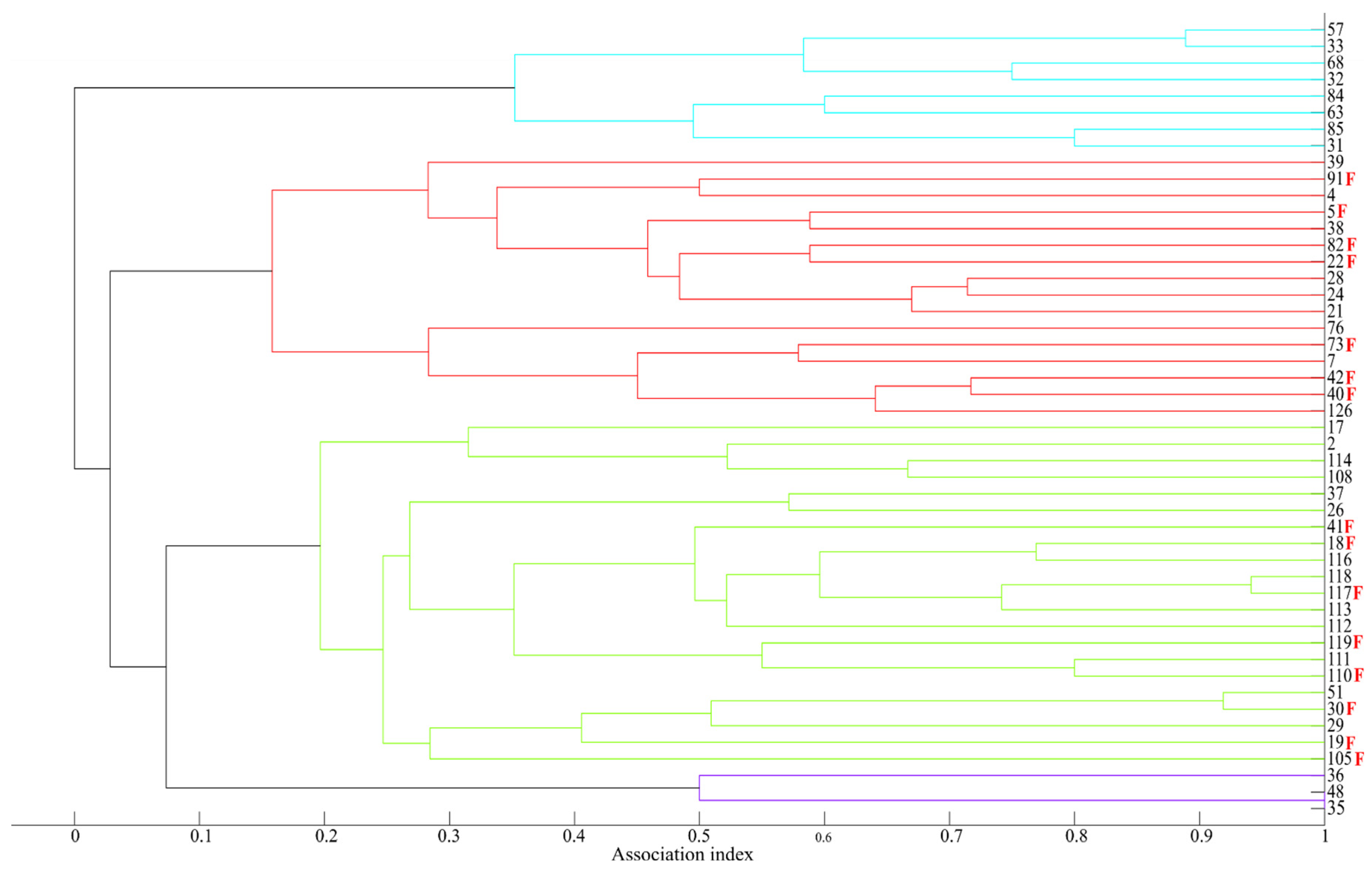
| Monthly Sighting Rate | Yearly Sighting Rate | Seasonal Sighting Rate | Relative Span Time | |||||||||||||
|---|---|---|---|---|---|---|---|---|---|---|---|---|---|---|---|---|
| Mean | Sd | Min | Max | Mean | Sd | Min | Max | Mean | Sd | Min | Max | Mean | Sd | Min | Max | |
| Cluster 1 (59 individuals) | 0.0322 | 0.0122 | 0.0256 | 0.0769 | 0.1111 | 0.0000 | 0.1111 | 0.1111 | 0.0549 | 0.0173 | 0.0476 | 0.0952 | 0.0034 | 0.0062 | 0.0000 | 0.0285 |
| Cluster 2 (20 individuals) | 0.2423 | 0.0663 | 0.1795 | 0.4103 | 0.5556 | 0.0883 | 0.4444 | 0.7778 | 0.3595 | 0.0567 | 0.2857 | 0.4762 | 0.6341 | 0.1596 | 0.3952 | 0.9903 |
| Cluster 3 (62 individuals) | 0.0877 | 0.0367 | 0.0513 | 0.1795 | 0.2778 | 0.0773 | 0.2222 | 0.4444 | 0.1452 | 0.0476 | 0.0952 | 0.2857 | 0.3696 | 0.2211 | 0.0901 | 0.8664 |
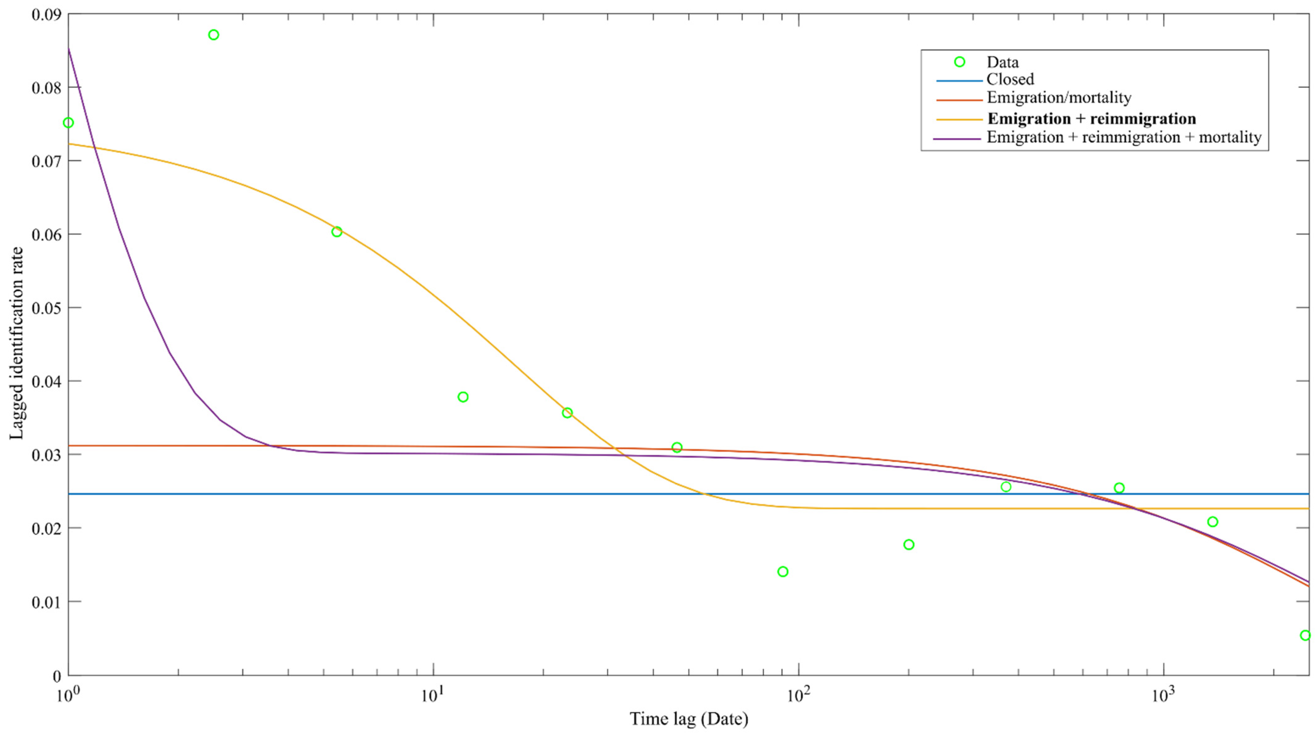
| Function Type | Explanation | QAIC | ΔQAIC |
|---|---|---|---|
| a1 | Closed | 9451.8 | 64.3 |
| a2*exp(−a1*td) | Emigration/mortality | 9411.0 | 23.5 |
| a2 + a3*exp(−a1*td) | Emigration + reimmigration | 9387.5 | |
| a3*exp(−a1*td) + a4*exp(−a2*td) | Emigration + reimmigration + mortality | 9399.7 | 12.2 |
| Mean HWI | |
|---|---|
| Cluster 1 | 0.06 ± 0.01 |
| Cluster 2 | 0.11 ± 0.02 |
| Cluster 3 | 0.14 ± 0.03 |
| Cluster 4 | 0.07 ± 0.01 |
| Mean HWI | |
| Cluster 1/Cluster 2 | 0.01 ± 0.03 |
| Cluster 1/Cluster 3 | 0.07 ± 0.03 |
| Cluster 1/Cluster 4 | 0.00 ± 0.00 |
| Cluster 2/Cluster 3 | 0.03 ± 0.03 |
| Cluster 2/Cluster 4 | 0.00 ± 0.00 |
| Cluster 3/Cluster4 | 0.00 ± 0.00 |
| Function Type | Explanation | QAIC | ΔQAIC |
|---|---|---|---|
| a1 | Pref. comps. | 6879.7 | 33.3 |
| a2*exp(−a1*td) | Casual acqs. | 6874.0 | 27.6 |
| a2 + a3*exp(−a1*td) | Pref. comps. + Casual acqs. | 6846.4 | |
| a3*exp(−a1*td) + a4*exp(−a2*td) | Two levels of casual acqs. | 6874.7 | 28.3 |
| Strength | Eigenvector Centrality | Reach | Clustering Coefficient | Affinity | |
|---|---|---|---|---|---|
| Overall | 5.33 ± 1.83 | 0.11 ± 0.09 | 31.74 ± 15.67 | 0.32 ± 0.09 | 5.64 ± 1.28 |
| Whitin clusters | |||||
| Cluster 1 (n = 3) | 3.01 ± 0.45 | 0.06 ± 0.02 | 15.04 ± 4.75 | 0.27 ± 0.02 | 4.92 ± 0.78 |
| Cluster 2 (n = 16) | 5.02 ±1.03 | 0.06 ± 0.03 | 27.49 ± 5.86 | 0.29 ± 0.06 | 5.47± 0.32 |
| Cluster 3 (n = 21) | 6.70 ± 1.54 | 0.20 ± 0.05 | 45.36 ±11.00 | 0.30 ± 0.06 | 6.76 ± 0.37 |
| Cluster 4 (n = 8) | 3.25 ± 0.46 | 0.00± 0.00 | 10.72± 1.34 | 0.48 ± 0.02 | 0.06 |
Publisher’s Note: MDPI stays neutral with regard to jurisdictional claims in published maps and institutional affiliations. |
© 2022 by the authors. Licensee MDPI, Basel, Switzerland. This article is an open access article distributed under the terms and conditions of the Creative Commons Attribution (CC BY) license (https://creativecommons.org/licenses/by/4.0/).
Share and Cite
Cipriano, G.; Santacesaria, F.C.; Fanizza, C.; Cherubini, C.; Crugliano, R.; Maglietta, R.; Ricci, P.; Carlucci, R. Social Structure and Temporal Distribution of Tursiops truncatus in the Gulf of Taranto (Central Mediterranean Sea). J. Mar. Sci. Eng. 2022, 10, 1942. https://doi.org/10.3390/jmse10121942
Cipriano G, Santacesaria FC, Fanizza C, Cherubini C, Crugliano R, Maglietta R, Ricci P, Carlucci R. Social Structure and Temporal Distribution of Tursiops truncatus in the Gulf of Taranto (Central Mediterranean Sea). Journal of Marine Science and Engineering. 2022; 10(12):1942. https://doi.org/10.3390/jmse10121942
Chicago/Turabian StyleCipriano, Giulia, Francesca Cornelia Santacesaria, Carmelo Fanizza, Carla Cherubini, Roberto Crugliano, Rosalia Maglietta, Pasquale Ricci, and Roberto Carlucci. 2022. "Social Structure and Temporal Distribution of Tursiops truncatus in the Gulf of Taranto (Central Mediterranean Sea)" Journal of Marine Science and Engineering 10, no. 12: 1942. https://doi.org/10.3390/jmse10121942
APA StyleCipriano, G., Santacesaria, F. C., Fanizza, C., Cherubini, C., Crugliano, R., Maglietta, R., Ricci, P., & Carlucci, R. (2022). Social Structure and Temporal Distribution of Tursiops truncatus in the Gulf of Taranto (Central Mediterranean Sea). Journal of Marine Science and Engineering, 10(12), 1942. https://doi.org/10.3390/jmse10121942