Article

On Sea-Level Change in Coastal Areas

by
Vincent Courtillot
1,
Jean-Louis Le Mouël
1,
Fernando Lopes
1,* and
Dominique Gibert
2
1
Institut de Physique du globe de Paris, Université de Paris, 75005 Paris, France
2
LGL-TPE, Université de Lyon 1, ENSL, CNRS, UMR 5276, 69622 Villeurbanne, France
*
Author to whom correspondence should be addressed.
J. Mar. Sci. Eng. 2022, 10(12), 1871; https://doi.org/10.3390/jmse10121871
Submission received: 2 November 2022 / Revised: 25 November 2022 / Accepted: 25 November 2022 / Published: 2 December 2022
(This article belongs to the Special Issue Late Quaternary Sea Level Changes: Causes, Patterns and Impacts)

Abstract

:
Variations in sea-level, based on tide gauge data (GSLTG) and on combining tide gauges and satellite data (GSLl), are subjected to singular spectrum analysis (SSA) to determine their trends and periodic or quasi-periodic components. GLSTG increases by 90 mm from 1860 to 2020, a contribution of 0.56 mm/yr to the mean rise rate. Annual to multi-decadal periods of ∼90/80, 60, 30, 20, 10/11, and 4/5 years are found in both GSLTG and GSLl. These periods are commensurable periods of the Jovian planets, combinations of the periods of Neptune (165 yr), Uranus (84 yr), Saturn (29 yr) and Jupiter (12 yr). These same periods are encountered in sea-level changes, the motion of the rotation pole RP and evolution of global pressure GP, suggesting physical links. The first SSA components comprise most of the signal variance: 95% for GSLTG, 89% for GSLl, 98% for GP and 75% for RP. Laplace derived the Liouville–Euler equations that govern the rotation and translation of the rotation axis of any celestial body. He emphasized that one must consider the orbital kinetic moments of all planets in addition to gravitational attractions and concluded that the Earth’s rotation axis should undergo motions that carry the combinations of periods of the Sun, Moon and planets. Almost all the periods found in the SSA components of sea-level (GSLl and GSLTG), global pressure (GP) and polar motion (RP), of their modulations and their derivatives can be associated with the Jovian planets. The trends themselves could be segments of components with still longer periodicities (e.g., 175 yr Jose cycle).

1. Introduction

A global rise in sea-level has become a topic of major concern for the both inhabitants of coastal areas and regions of very low altitude and a huge amount of studies have been devoted to the description and understanding of evolutions in global sea-level. The problem is sometimes confusing because the definition of sea-level rise (and drop) is not always clear and unique and the observations on which it is based have been obtained by very different methods (tide gauges, GPS measurements, satellite observations). Referring to works by [1,2,3,4,5,6], we define absolute the sea-level SL(P,t) as the difference between (1) the distance from the center of mass of the Earth to the sea surface, at time t and location P, and (2), the distance from the center of mass of the Earth to the sea bottom (solid Earth), which is the water depth, at the same time t and location P:
SL ( P , t ) = R s s ( P , t ) R s e ( P , t )
The evolution of sea level between time t and a reference time t r is simply:
SLE ( P , t ) = SL ( P , t ) SL ( P , t r ) = [ R s s ( P , t ) R s e ( P , t ) ] [ R s s ( P , t r ) R s e ( P , t r ) ]
which can be rearranged as:
SLE ( P , t ) = [ R s s ( P , t ) R s s ( P , t r ) ] [ R s e ( P , t ) R s e ( P , t r ) ]
In that form, changes in sea level are the difference between the changes in altitude of the sea surface (i.e., the geoid), which are measured by tide gauges in coastal areas and changes in the altitude of the solid Earth that can be measured at GPS stations (e.g., [7,8]). The geoid term [ R s s ( P , t ) R s s ( P , t r ) ] is modeled as: G γ ( P , t ) + c ( t ) , where G is the full gravitational potential G gravity at the Earth surface and c(t) stands for changes in masses at the surface, including ice melting [9].
Despite the actual complexity of the consequences of the (apparently simple) law of attraction of masses, Laplace [10] was able to build a full theory of celestial mechanics. He wrote a whole volume (the book IV of their Treatise) on the oscillations of the sea and of the atmosphere. Laplace showed that, in order for sea-level to be in equilibrium, the sum of forces had to be zero, eventually resulting in the famous Liouville–Euler system of partial differential equations. Tides were understood to be second-order oscillations, whose phases and amplitudes could be computed. The mathematical stage was set for the study of changes in sea-level.
The early 1930s saw a period of active interest in the determination of sea level and its changes, and the physical causes of these changes. Nomitsu and Okamoto [11] attributed SL variations in the Sea of Japan to variations in density and atmospheric pressure. Marmer [12] noted an annual oscillation at the tide gauges of Seattle and San Francisco that he also linked to meteorological phenomena. After a decade of additional observations, Jabobs [13] and LaFond [14] concluded that there was indeed a general rise in sea-level. Several explanations were considered: insulation from the Sun, meteorological tides, water density, changes in geography and geology of ocean basins. None was found to be completely satisfactory. McEwen [15] envisioned a complex mechanism with evaporation in the summer and precipitation in winter affecting the global sea-level. Further study showed that these annual variations were in fact in the phase in all observation stations, and the idea had to be dropped. Only the pressure patterns and hence the winds remained as a potential cause of periodic SL variations.
By the end of the 1970s and early 1980s, the principal cause of sea-level rise came to be attributed to a major phase of warming having resulted in the melting of the northern hemisphere ice caps. Refs. [16,17] elaborated on the theory of post-glacial isostatic rebound. The global warming of the atmosphere that took place over the past 150 years or so was attributed to anthropic release of greenhouse gases, contributing to the melting of glaciers and a rise in SL [18,19,20,21,22,23,24,25].
Our knowledge of sea-level and its variations in the 19th century and up to the present is primarily based on observations made by tide gauges. These provide the first half of Equation (3), that is [ R s s ( P , t ) R s s ( P , t r ) ] . One of the longest series comes from the Brest (France) tide gauge, established in 1807 and still in function. Le Mouël et al. [26] recently analyzed the Brest data and in parallel Earth’s pole positions (from the IERS, 1845–2019), submitting both of them to singular spectral analysis (SSA). The first SSA components of both series, i.e., the trends, are very similar, with a major acceleration event near 1900 and a sea-level lagging pole motion by 5–10 years. SSA components with periods 1 yr, ∼11 yr and 5.4 yr are common to the two series. An important feature is a 0.5 yr component that is present in sea-level but absent from pole motion. The remarkable similarity of the two trends and their phase lag suggests a causal relationship opposite to what is generally accepted.
The primary aim of the present paper is to apply the same analysis to the global database of tide gauges. The tide gauge data are maintained by the Permanent Service of Mean Sea Level (PSMSL, https://www.psmsl.org/data/obtaining/complete.php (accessed on 5 July, 2020). Measurements of coastal sea level are available at 1548 sites; the raw data at all sites are shown in Figure 1.
The second half of Equation (3), that is, vertical land motion VLM = [ R s e ( P , t ) R s e ( P , t r ) ] , can be accessed through GPS measurements. These allow far better coverage of Earth surface but cover a much shorter span of time, generally 30 yr at most. For that reason, only “recent” trends covering that period can be accessed. A very thorough analysis of these data has recently been published by [8]. The database is maintained by the Nevada Geodetic Laboratory, with 19286 sites scattered throughout the globe, and is called Median Interannual Difference Adjusted for Skewness (MIDAS, http://geodesy.unr.edu/velocities/ (accessed on 5 July 2020).
Since the beginning of the 1990s, the sea level has also been monitored by series of altimetric satellites that have allowed much denser global coverage but (as is the case for GPS measurements) over a short time range of 30 years. A number of recent papers have attempted to combine these very different data sets, resulting in various global sea-level (GSL) curves (e.g., [8,27]). Interest in these GSL curves has focused on their trends, acceleration, annual and inter-annual variations, and on the mechanisms responsible for these variations.
We recently successfully applied the SSA method (see Golyandina and Zhigljavsky [28], Lemmerling and Van Huffel [29], Golub and Reinsch [30]) to a number of geophysical and heliophysical time series. SSA decomposes any time series into a sum of components, a trend (that may or may not be present) and stationary quasi-periodic components. We have explained the method in a number of papers [31,32]. For instance, oscillations (pseudo-cycles) of ∼160, ∼90, ∼60, ∼22 and ∼11 yr are found in a series of sunspot numbers (e.g., Refs. [33,34,35,36,37,38,39]) as well as in a number of terrestrial phenomena [31,32,40,41,42,43,44,45,46,47,48,49,50,51,52,53], particularly sea level [26,54,55,56,57]. These particular periods (or periodicities) are of special interest, as they are members of the family of commensurable periods of the Jovian planets acting on the Earth and Sun [39,41,49,51,58]. These values are indeed close to the revolution periods of Neptune (165 yr), Uranus (84 yr), Saturn (29 yr) and Jupiter (12 yr) and several of their commensurable periods (see Table 1 in [51]).
In Section 2 of this paper, we discuss the tide gauge records and perform an SSA of these. In Section 3, we discuss and analyze the time series of vertical land motion (VLM) based on GPS measurements. In Section 4, we submit some global sea-level (GSL) curves that include satellite observations to SSA. We compare and discuss the results of these analyses in Section 5 and conclude in Section 6.

2. SSA of Tide Gauge Records Time Series (i.e., [ R ss ( P , t ) R ss ( P , t r ) ]

Drawing on a recent paper [26], in which we analyzed the record from the Brest tide gauge since 1807, using SSA to extract its main components, we proposed to build a global sea-level curve covering the past 200 years using data from tide gauges only (GSLTG). We are aware of the uncertainties due to geography and tectonics but are interested in subjecting the original data to as little manipulation as possible.
We have selected the recordings from 31 stations (Table 1) on the basis of two criteria: the longest possible span of time and the best possible—if still too restrained—spatial coverage (Figure 2).
We have also performed the analyses that follow on the full database (1548 tide gauge stations): this results in increased dispersion without changing what can be drawn from the selection of 31 stations. The raw data from the 31 stations are all displayed without any filtering or processing, except for the fact that the first value has been subtracted, so that all series begin with a zero and only relative vertical variations of SL are displayed (Figure 3).
The two tide gauges that have large slopes (plotted in green in Figure 3), one positive (Manila, S. Harbor, Philippines) and one negative (Churchill, Canada), outline a funnel shape (see Table 1). The funnel undergoes rapid growth after 1950, with a total amplitude of 2 m, determined by the two extrema at Manila and Churchill. The annual oscillation, first identified by Marmer [12], has an amplitude in the order of 200 mm (peak to trough) for all tide gauges. The individual data points are shown in Figure 4a.
We then determine a smooth mathematical model of the mean sea-level variations as a function of time, in a least squares sense (e.g., [59]). For a mathematical representation of this smooth model, we can choose between polynomials, sine functions, exponentials, or splines. We select sine functions, based on our previous experience with the Brest data [26]. We add sine components progressively, until no more significant information is brought by the new component (in the sense of the Akaike criterion, see [60] used in [45]). In the present case, this leads to a model consisting of eight sine components. This model is shown with the data in Figure 4a and enlarged in Figure 4b.
The model of Figure 4a represents the mean variation common to all 31 tide gauges. At first glance, it consists of an annual oscillation, with a peak to trough amplitude of approximately 100 mm and a rather constant overall mean value. Figure 4b shows more precisely the modulations of this amplitude. The remaining scatter of data points can be assigned to local or regional variability. We call this model GSLTG. The GSLTG curve is then analyzed using SSA. The analysis yields a sum of components with (pseudo-) periods of 1 yr, 90 yr, 60 yr, 80 yr, 0.5 yr and 20 yr (in order of decreasing amplitudes). These are shown (in order of decreasing period) in Figure 5 (see also Table 2). The leading annual component has an amplitude (peak to trough) of 80 mm and undergoes a (longer than centennial) modulation with 10 mm amplitude. The next two components (90 and 80 yr) both have an amplitude of 40 mm, and the next three of approximately 15 mm. Taken together, they capture 95% of the total variance. The trend itself can be modeled with only three sine functions with periods 90, 60 and 20 yr.

3. Introducing the GPS Vertical Land Motion Time Series (the [ R se ( P , t ) R se ( P , t r ) ]

As noted above, the GPS data series of VLM are all shorter than 30 years, which makes it impossible to directly combine them with the tide gauge data that are far longer on average and allow one to explore much longer periods. Unable to do better, one can at least calculate a recent (present) trend, applying a simple linear regression to the GPS data. Furthermore, a simple linear regression of all the series shown in Figure 3 allows a comparison and combination of the gauge and VLM data: Figure 6 shows the respective histograms of the slopes of the 1548 gauges and of the GPS at the same (or close by) coastal locations (Figure 7). The median for tide gauges is +2.0 mm/yr and 92.7 % of gauges have slopes between −10 and +10 mm/yr; the median for VLM is −0.6 mm/yr and 96.0 % of the values are between −10 and +10 mm/yr. The locations and values of the tide gauges and the VLM are plotted, respectively, in Figure 7a,b. Over a large part of the coastal areas, the tide gauge signal and the VLM appear to be opposite in sign, that is, anti-symmetrical (e.g., North America, the Mediterranean region). The results of this analysis are in full agreement with the thorough study of [8], in which water rises as the land tends to subside and vice versa.
If we assume that the recent (30 yr) VLM in Brest remained the same from 1807 to the present, then we can evaluate the mean sea level rise with respect to the Earth’s center of mass (Equation (3)) as 1.5 mm/yr. This rough estimate is in full agreement with a series of recent studies (e.g., [8,26,57,61,62,63,64].
The MIDAS database provides the slopes of the GPS data over their duration (life time), which can range from 2 to over 20 years. The authors in [8] argue that, apart from tectonic events, these give an accurate depiction of VLM. For each tide gauge, we fit straight line segments to sea level data in the same way (though over a much longer duration, between 3 and 217 years).

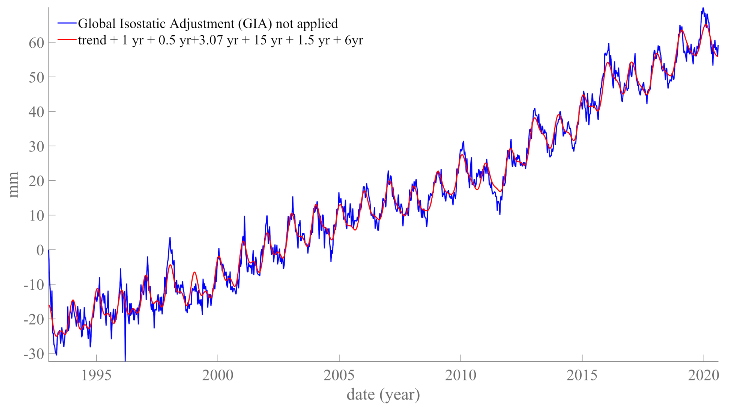
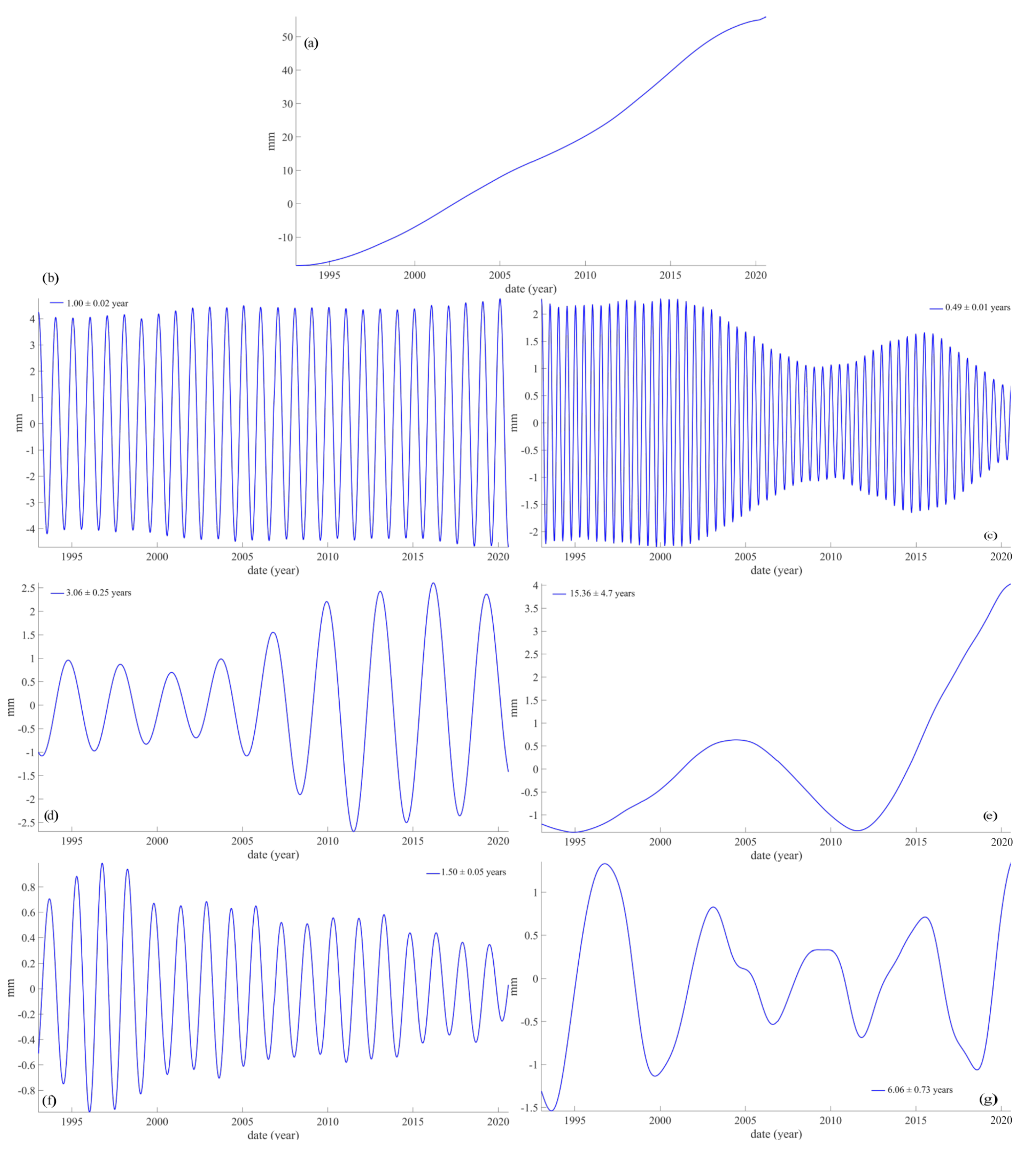
4. SSA of GSL Curves Obtained with Inclusion of Satellite Data

As far as we are interested in the long-term rise in sea level and its quasi-periodic components, but do not have VLM data over this long term, we can still use SSA to analyze a number of global sea-level curves available from the literature.
We select first that by [27], Figure 8. These authors estimated the rise in global average sea level from a combination of satellite altimeter data for the period 1993–2009 with coastal and island sea-level (tide gauge) measurements from 1880 to 2009. Variations in GSL as a function of time are provided by NASA (https://podaac-tools.jpl.nasa.gov/drive/files/allData/merged$_$alt/L2/TP$_$J1$_$OSTM/global$_$mean$_$sea$_$level/GMSL$_$TPJAOS$_$5.0$_$199209$_$202008.txt (accessed on 5 July, 2020). The SSA of the resulting curve GSLl (l for long) yields a trend and components at 54.5 ± 8.7, 19.4 ± 1.7, 10.1 ± 0.6, 3.9 ± 0.1 and 31.0 ± 5.5 yr (Table 2 and Figure 9) in order of decreasing amplitude (or roughly, given the uncertainties trend, 60, 20, 11, 4 and 30 yr). These components are shown in Figure 09 (in order of decreasing period); their sum amounts to 89.4% of the series total variance (Figure 8). The 3.9 yr component could correspond to the second harmonic of the Schwabe cycle [38]. Note that the prominent 1 and 0.5 yr variations have been filtered out by [27].
Since the 1880–2009 GSLl incorporates two very different data sets (measurements from tide gauges and satellites), we have resumed the analysis for the 1993–2009 GSLs (s for short) based on satellite data only. For details on the structure of the data, we refer the reader to [65]. For explanations on how the data set has been created from 27 years of altimetric measurements by the successive satellites TOPEX/Poseidon (T/P), Jason-1, Jason-2 and Jason-3, we refer the reader to [66,67]. The global mean sea-level data consist in several sets of time series, some with a “Global Isostatic Adjustment applied”, and some “GIA not applied”. The latter (without GIA) is shown in Figure 10, from January 1993 to August 2020, with a sampling interval of 9.92 days.
The SSA of the resulting curve GSLs yields a trend and components at 1.00 ± 0.02, 0.49 ± 0.01, 3.06 ± 0.25, 15.4 ± 4.7, 1.50 ± 0.05 and 6.06 ± 0.73 yr in order of decreasing amplitude (or roughly, given the uncertainties trend, 15-20, 6, 3, 1.5, 1 and 0.5 yr). These components are shown in Figure 11 (in order of decreasing period); their sum amounts to 87.3% of the series total variance (Figure 10). The sum of the seven first components extracted by SSA is plotted as a red curve. The 6.1, 3.1 and 1.5 yr quasi periods could correspond to the harmonics of the Schwabe cycle (cf. [38], Table 1).

5. Discussion

5.1. Components Shared by GSLl, GSLTG and SSN

Despite the fact that one is included in the other, the GSLl and GSLs series do not share many characteristics (cf. Table 2). Their trends are similar and they both have significant 1-year and 6-month components, but the two series do not share other quasi- periodic components (unless the 15-year component of GSLs can be considered to be the same as the 20 yr component of GSLl, given uncertainties). Actually, the span of the GSLs data is only 27 yr and should not be used to identify components with periods longer than, say, 27/2 or ∼15 yr.
In stark contrast, GSLl shares seven components with GSLTG: a trend of 60, 30, 20, 10, 1 and 0.5 yr components cf. Table 2).
Le Mouël et al. [48] and Courtillot et al. [39] have calculated the SSA components of the sunspot number SSN, a characteristic of solar activity. Four components of SSN are found in GSLl (60, 30, 20, 10 yr) and six in GSLTG (90, 60, 20, 30, 10, 5 yr), taking into account the uncertainties (fi. 10.15 ± 0.58 and 10.64 ± 1.17 are both considered equivalent to the SSN packet at 10.6 and 11.3 yr).
A puzzling observation is that the amplitude of the annual component of GSLs is only 8 mm peak to trough (Figure 11b), when tide gauges record a mean amplitude an order of magnitude larger (80 mm; Figure 5a). This could be due to the fact that tide gauges are located in shallow waters where wave amplitude is amplified; in any case, this is where the sea-level is relevant to human activities. The trend amplitude between 1860 and 2020 is 80 mm for GSLTG (Figure 4b) and more than 200 mm for GSLl (Figure 8). Moreover, with a GSLTG curve extending over two centuries, we see that the trend of the shorter series GSLs could actually be part of a longer cycle (in the same order as the ∼90 year Gleissberg cycle).

5.2. Comparison with Global Pressure GP

Thus, SSA reveals that GSLl and GSLTG share many characteristics that could constrain the mechanisms that control both series of sea-level change. In order to strengthen this hypothesis, one can try to find whether some other geophysical phenomenon would possess similar characteristic features with the same spectral signatures. We have searched whether the Earth’s global mean pressure (GP) meets these requirements. A series of monthly mean atmospheric pressure (everywhere in the world) is available was of 1846 [68]. It can be accessed through the Met Office Hadley Centre (http://www.metoffice.gov.uk/hadobs/hadslp2/data/download.html accessed on 5 July 2020) website under the name HadSPL2. Following Laplace’s work on the subject of the spatial and temporal stability of pressure ([10], book IV, chap 4, page 294), we built a series of monthly global pressure GP and submitted it to SSA: the first four components, i.e., the trend followed by periods of 1 yr, 6 months and ∼25 yr, account for 98% of the total variance. Thus, GSLTG and GP share three major components at ∼20/25 yr, 1 yr and 6 months. Comparisons between some features of GSLTG and GP are illustrated in Figure 12. The annual and semi-annual components match in phase and frequency and are slightly modulated with a time constant in the order of a century or more. Both series have ∼20/25 yr components that drift, one with respect to the other. Interestingly, the derivative of the trend of pressure GP matches the trend of GSLTG, suggesting a relation of the form GSLTG∼ (d/dt) GP. Furthermore, the ratios of the amplitudes of the various SSA components of GSLTG and GP are approximately constant (Table 3). Sea level and pressure respond in similar ways at all time scales.

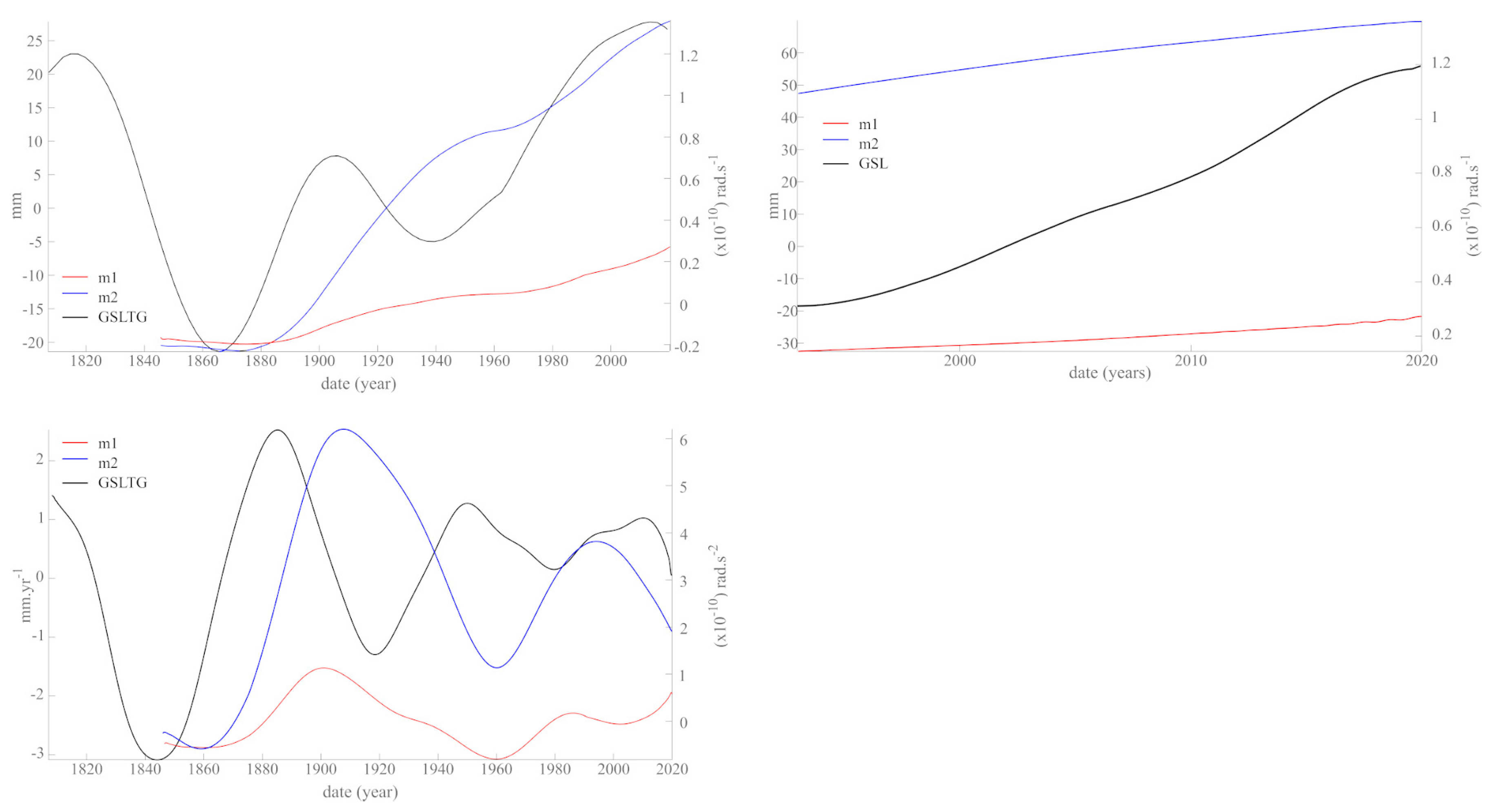
5.3. Comparison with the Mean Motion of the Rotation Pole (RP)

It is generally accepted (e.g., [17]) that the mean motion of the rotation pole (RP) and the mean sea-level (be it GSLTG or GSL) belong to the same family because of the reorganization of surface masses due to pole motion. Because the Liouville–Euler equations are a linear differential system of second order, one understands the resemblance between RP and both GSLTG or GSL, at least during longer periods. Can the analysis of the RP series bring additional light to the question of the forcing of sea level (we refer the reader to earlier work on polar motion by [31,32,51])?
The series of data describing the rotation pole coordinates (RP) is maintained by the International Earth Rotation and Reference Systems Service (IERS, https://www.iers.org/IERS/EN/DataProducts/EarthOrientationData/eop.html accessed on 5 July 2020). Two series of measurements of pole coordinates m 1 and m 2 are provided by IERS under the codes EOP-C01-IAU1980 and EOP-14-C04. The first one runs from 1846 to 1 July 2020 with a sampling rate of 18.26 days, and the second runs from 1962 to 1 July 2020 with daily sampling. Figure 13 displays the trends (top) and derivatives (bottom) of the rotation pole (RP) coordinates m 1 and m 2 together with those of GSLTG (1807–2020). There is a suggestive anti-correlation between the trend of GSLTG and the derivative of the trend of m 2 (GSLTG∼(d/dt) RP), with the former leading the latter by several decades (Figure 13, lower left). This behavior was noted for the Brest tide gauge by [32]. This is yet another line of observational evidence that the sea-level curve based on tide gauges has an underlying physical mechanism.
The three main components of pole motion RP, i.e., the Markovitch drift, the Chandler free oscillation (that has never yet been detected in sea level) and the annual forced oscillation, carry more than 75% of the signal’s total energy (variance) [31,51,53]. Ref. [31] also showed the presence of other components at 22 yr (Hale), 11 yr (Schwabe) and a 5.5 yr harmonic. The order of magnitude of these solar components is 10 12 to 10 14 rad.sec 1 , that is 1–4 orders of magnitude smaller than the main components (10 11 to 10 10 (rad· sec) 1 ). In [26,39,51], it has been shown that the derivative of the Markovitch component includes the 90 yr (Gleissberg) cycle as its trend. Ref. [51] identified some other components that also appear in the SSN sunspot series [39]. We limit ourselves to the shared (quasi-) periods of 90, 22, 11, 5.5, 1.4 and 1 year.

5.4. The Liouville–Euler System and Solar Components in Sea Level

The Liouville–Euler system of equations can be written (cf. [9]; chapters 3 and 4):
( 1 / σ r ) d m d t + m = f d m 3 d t = f 3
d m d t = m 1 + i m 2 , where ( m 1 , m 2 ) are the coordinates of motion of the Earth’s rotation pole (RP) and f = f 1 + i f 2 and f 3 are the excitation functions. These are explicitly written in [9], chapter 4, system 4.1.1, page 47. These functions belong to three distinct families: masses, motions (of masses), and imposed forces (torques). Parameters ( m 1 , m 2 , m 3 ) provide a global scalar for pole motion, and the excitation functions are also global. Because coupled system (4) is linear, any periodic component found in ( m 1 , m 2 , m 3 ) data/observations must also be present in ( f 1 , f 2 , f 3 ).
If system (4) does apply, since variations in sea-level are the motion part of the excitation functions, and since the Gleissberg cycle (90 yr) and annual components have been found, one should also find 1.4 yr component. In the same way, Moreira and Cazenave [69] identified an 11 yr oscillation, Jevrejeva et al. [54] a 22 yr oscillation and Chambers [55] another one at 60 yr (solar, cf. [39]) with weak amplitude in polar motion (cf. [51,53]). Thus, cycles that are commonly associated to the Sun are also detected in sea level, though they are a very weak component of polar motion.

5.5. Planetary Forcings

Laplace predicted that all terrestrial masses should be under the influence of other celestial bodies, at much longer periods (though he did not have the data to demonstrate it experimentally). For these longer durations, planets were the potential culprits. If one studies durations that are short compared to a decade, the 11 yr component will be included in the trend. In the same way, if one looks at the variations shorter than 5 days, the 28 day lunar cycle will be included in the trend. This is particularly true for fluid envelopes. In [39], we showed that sunspots, which move on the external fluid envelope of the Sun, include components with periods that can be linked to planetary ephemerids (commensurable periods of the Jovian planets), as proposed by [41], namely ∼ 165 yr (José cycle, associated with Neptune), ∼90 yr (Gleissberg cycle, associated with Uranus), ∼30 yr (Saturn), ∼ 22 yr (Hale cycle, a Jupiter/Saturn commensurability), ∼ 11 yr (Schwabe cycle, associated with Jupiter), etc. See Lopes et al. ([70]) for more details.
The solid Earth acts as an integrator (e.g., [9], Chapter 3) at the longer periods (e.g., [51]), but reacts almost instantaneously to the shorter periods (e.g., [71]). The effects are large in the former case, but less so in the latter. As pointed out by [10], Book IV, Chapters 4 and 5, because the atmosphere and oceans are fluids with low viscosity, they actually behave as solid envelopes at the longer periods. This is for instance the reason why the annual oscillations observed on tide gauges (Figure 11) have similar amplitudes. To this response is added the response described by the Liouville–Euler equations. It is used for instance by [17], who considered that there is a reorganization of surface masses when the inclination of the Earth’s rotation axis evolves in space. External forces influence polar motion and this should also be seen in sea-level and pressure. We do find the signatures of these influences in the trends (directly or through their derivatives) the most energetic components. The apparent rise of the sea-level is similar to the pattern of polar motion: this is why, like others, we find this funnel pattern of tide gauges. The mass of the system is constant; this agrees with the fact that the pressure variation remains constant and linked with the sea-level. Under the hypothesis of common external forcing (common to the solid Earth and its fluid envelopes) this would explain why the derivative of the trend of GP (with the sign reversed) and the trend of GSLTG match quite well (Figure 12, middle left).

6. Summary and Concluding Remarks

In the present paper, we have first analyzed variations in the geoid, using tide gauge data for the time span 1807–2020 (GSLTG) and variations in the global sea level combining tide gauges and satellite data (GSLl [27]); then, with much better spatial coverage but a much more restricted time span (1993-2020), satellite-only data (GSLs, [65]). Our main goal has been to determine the trends and successive periodic or quasi-periodic components of these time series, using the SSA method (SSA) that we have used, with interesting results, in a series of previous papers [26,31,39,47,48,51].
Since satellite data are first corrected using tide gauges, we analyzed the tide gauge data at 71 gauge stations separately (series GSLTG). We see all kinds of behavior, with increasing, stable or decreasing mean values (trend), giving the complete data set a funnel shape. The resulting GLSTG mean oscillates around an almost constant value. From 1860 to 2020, the trend increases by 90 mm, or a contribution to the mean rise rate of 0.56 mm/yr.
Our observations are compatible with previous results also based on tide gauge data but using different methods: [19] Figure 02, [72] Figures 9.1 and 9.2 and [24] Figure 03 show the funnel-shaped distribution of the data with values in agreement with GSLTG.
SSA analysis of the GSLTG series identifies components with celestial periods already found when analyzing the Brest tide gauge data [26]. We have shown (Table 3) that the ratios of amplitudes of SSA components (trend, 20–30 yr, 1 yr, 0.5 yr) of GSLTG vs. global pressure GP are almost constant (at 0.02 hPa/mm). This observation supports the idea that tide gauge data contain significant information on the physical links between mean pressure and (geoid) sea-level.
The longer (annual to multi-decadal) periods we encountered in the GSLTG and GSLl sea-level curves in the present study have already been encountered in a number of geophysical and heliophysical time series. These periods (or quasi-periods) are ∼80–90, 60, 30, 20, 10–11, and 4–5 years. They can be compared to the commensurable periods of the Jovian planets acting on the Earth and Sun as proposed by [41]. The combination of the revolution periods of Neptune (165 yr), Uranus (84 yr), Saturn (29 yr) and Jupiter (12 yr) and several commensurable periods makes additional pseudo-cycles of 60 and 20 yr appear in sunspots [32,39] as well as in a number of terrestrial phenomena [31,32,41,45,46,49,51,58], particularly in sea level [55,73,74,75,76]. It is therefore not a surprise to find Jovian periods in GSLTG. Even trends could be part of commensurate cycles longer than the time span over which the data are available.
The (often joint) periods encountered in the sea-level changes, the motion of the rotation pole RP and the evolution of global pressure GP and the relations between some of their trends (as determined using SSA) suggest that there may be physical links and causal relationships between these geophysical phenomena and the time series of observations available. The ubiquitous presence of many common components in the variations of many natural phenomena (that a priori might seem largely unrelated) has led us to return to the general forcing envisioned by [10] and to the full theory he developed. In their 1799 Treatise of Celestial Mechanics, Laplace derived the Liouville–Euler partial differential equations that describe the rotation and translation of the rotation axis of any celestial body, and showed that the only thing that influences the rotation of celestial bodies is the action of other celestial bodies. Laplace emphasized that one must consider the orbital kinetic moments of all planets in addition to gravitational attractions and concluded that the Earth’s rotation axis should undergo motions with components that carry the periods or combinations of periods of the Sun, Moon and planets (particularly Jovian planets).
In [51,53], we tested Laplace’s theoretical results using observations that have accumulated since their time. In [39], we gave evidence of the driving influence of the planets (mainly the Jovian planets) on the Earth’s rotation axis [51], and on solar activity, through exchanges of angular momentum. In the present paper, we have extended the analysis to changes in global sea-level, as measured by tide gauges (GSLTG), and we have also shown that there were several shared periodic components with global pressure GP and the Earth’s rotation axis RP.
Laplace’s treatment shows that the kinetic moments of planets act both directly on the Earth and on the Sun’s fluid external layers, and perturb its rotation; hence, its revolution and eventually the Earth’s axis of rotation RP. The SSA analysis of the envelopes of the derivatives of the three first polar motion components yields a number of additional periods that belong to the series of commensurable periods, among which 70 yr, 60 yr (Saturn; also found in global temperatures and oceanic oscillations), 40 yr (a commensurable revolution period of the four Jovian planets), 30 yr (Saturn) and 22 yr (Jupiter and Solar). The same is true for the first three SSA components of sunspot series SSN (trend or Jose 175 year cycle, linked to Neptune; 11 yr Schwabe cycle, linked to Jupiter; and 90 yr Gleissberg cycle, linked to Uranus). Almost all the (quasi-) periods found in the SSA components of sea-level (GSLl and GSLTG), global pressure (GP) and polar motion (RP) of their modulations and of their derivatives can be associated with Jovian planets (Table 3). These complement the list of SSA quasi-periodic and periodic components that are found in GSLl, GSLTG, GP, RP and SSN (90, 60, 30, 20, 10, 5, 1 and 0.5 years) and can all be associated with planetary forcings, as envisioned by Laplace. In particular, planetary forcing factors are likely causally responsible for many of the components of sea-level variations as measured by tide gauges. It is of particular interest to search for high-quality data series on longer time intervals, that can allow one to test whether the trends themselves could be segments of components of even longer periodicities (e.g., 175 yr Jose cycle). In any case, the first SSA components of the series analyzed in this paper comprise a large fraction of the signal variance: 95% for the first six components of GSLTG, 89% for the first six components of GSLl, 87% for the first six components of GSLs, 98% for the first four components of GP and 75% for the first three components of RP. It is clear that one should attempt to physically model these series with this set of periods (SSA components) before trying to invoke alternate sources (forcing functions).

Author Contributions

V.C., J.-L.L.M., F.L. and D.G. contributed to conceptualization, formal analysis, interpretation and writing. All authors have read and agreed to the published version of the manuscript.

Funding

This research was supported by the Université de Paris, IPGP and the LGL-TPE de Lyon.

Data Availability Statement

The used data are freely available at the following address: Permanent Service of Mean Sea Level: https://www.psmsl.org/data/obtaining/complete.php accessed on 5 July 2020; Median Interannual Difference Adjusted for Skewness: http://geodesy.unr.edu/velocities/ accessed on 5 July 2020; NASA: https://podaac-tools.jpl.nasa.gov/drive/files/allData/merged$_$alt/L2/TP$_$J1$_$OSTM/global$_$mean$_$sea$_$level/GMSL$_$TPJAOS$_$5.0$_$199209$_$202008.txt accessed on 5 July 2020; Met Office Hadley Centre: http://www.metoffice.gov.uk/hadobs/hadslp2/data/download.html accessed on 5 July 2020; International Earth Rotation and Reference Systems Service: https://www.iers.org/IERS/EN/DataProducts/EarthOrientationData/eop.html accessed on 5 July 2020.

Acknowledgments

We thank the anonymous reviewers for their helpful comments on the manuscript.

Conflicts of Interest

The authors declare that they have no known competing financial interest or personal relationships that could have appeared to influence the work reported in this paper.

References

  1. Farrell, W.E.; Clark, J.A. On post glacial sea level. Geophys. J. Int. 1976, 46, 647–667. [Google Scholar] [CrossRef]
  2. Wu, P.; Peltier, W.R. Glacial isostatic adjustment and the free air gravity anomaly as a constraint on deep mantle viscosity. Geophys. J. Int. 1983, 74, 377–449. [Google Scholar] [CrossRef] [Green Version]
  3. Mitrovica, J.X.; Milne, G.A. On post-glacial sea level: I.General theory. Geophys. J. Int. 2003, 154, 253–267. [Google Scholar] [CrossRef] [Green Version]
  4. Spada, G.; Stocchi, P. The Sea Level Equation, Theory and Numerical Examples; Aracne online edition 2006; Aracne Editrice: Roma, Italy, 2006; pp. 1–96. ISBN 10 8854803847. [Google Scholar]
  5. Spada, G.; Stocchi, P. SELEN: A Fortran 90 program for solving the sea-level equation. Comput. Geosci. 2007, 33, 538–562. [Google Scholar] [CrossRef]
  6. Spada, G.; Melini, D.; Galassi, G.; Colleoni, F. Modeling sea level changes and geodetic variations by glacial isostasy: The improved SELEN code. arXiv 2012, arXiv:1212.5061. [Google Scholar] [CrossRef]
  7. Blewitt, G.; Kreemer, C.; Hammond, W.C.; Gazeaux, J. MIDAS robust trend estimator for accurate GPS station velocities without step detection. J. Geophys. Res. Solid Earth 2016, 121, 2054–2068. [Google Scholar] [CrossRef] [Green Version]
  8. Hammond, W.C.; Blewitt, G.; Kreemer, C.; Nerem, R.S. GPS Imaging of Global Vertical Land Motion for Studies of Sea Level Rise. J. Geophys. Res. Solid Earth 2021, 126, e2021JB022355. [Google Scholar] [CrossRef]
  9. Lambeck, K. The Earth’s Variable Rotation: Geophysical Causes and Consequences; Cambridge University Press: Cambridge, UK, 2005. [Google Scholar]
  10. Laplace, P.S. Traité de méCanique céLeste; de l’Imprimerie de; Crapelet: Paris, France, 1799. [Google Scholar]
  11. Nomitsu, T.; Okamoto, M. The causes of the annual variation of the mean sea level along the Japanese coast. Mem. Coll. Sci. Kyoto Imp. Univ. Ser. 1927, 10, 125–161. [Google Scholar]
  12. Marmer, H.A. Tidal Datum Planes; US Government Printing Office: Washington, DC, USA, 1927; p. 135.
  13. Jacobs, W.C. Sea level departures on the California coast as related to the dynamics of the atmosphere over the North Pacific Ocean. J. Mar. Res. 1939, 2, 181–194. [Google Scholar] [CrossRef]
  14. LaFond, E.C. Variations of sea level on the Pacific coast of the United States. J. Mar. Res. 1939, 2, 17–29. [Google Scholar] [CrossRef]
  15. McEwen, G.F. Some Energy Relations between the Sea Surface and the Atmosphere; Yale Univ: New Haven, CT, USA, 1937. [Google Scholar]
  16. Peltier, W.R.; Andrews, J.T. Glacial-isostatic adjustment—I, The forward problem. Geophys. J. Int. 1976, 46, 605–646. [Google Scholar] [CrossRef]
  17. Nakiboglu, S.M.; Lambeck, K. Deglaciation effects on the rotation of the Earth. Geophys. J. Int. 1980, 62, 49–58. [Google Scholar] [CrossRef] [Green Version]
  18. Etkins, R.; Epstein, E.S. The rise of global mean sea level as an indication of climate change. Science 1982, 215, 287–289. [Google Scholar] [CrossRef]
  19. Gornitz, V.; Lebedeff, S.; Hansen, J. Global sea level trend in the past century. Science 1982, 215, 1611–1614. [Google Scholar] [CrossRef]
  20. Lambeck, K.; Nakiboglu, S.M. Recent global changes in sealevel. Geophys. Res. Lett. 1984, 11, 959–961. [Google Scholar] [CrossRef]
  21. Meier, M.F. Contribution of small glaciers to global sea level. Science 1984, 226, 1418–1421. [Google Scholar] [CrossRef]
  22. Peltier, W.R.; Tushingham, A.M. Global sea level rise and the greenhouse effect: Might they be connected? Science 1989, 244, 806–810. [Google Scholar] [CrossRef] [PubMed]
  23. Douglas, B.C. Global sea level rise. J. Geophys. Res. Oceans 1991, 96, 6981–6992. [Google Scholar] [CrossRef] [Green Version]
  24. Douglas, B.C. Global sea level acceleration. J. Geophys. Res. Oceans 1992, 97, 12699–12706. [Google Scholar] [CrossRef] [Green Version]
  25. Douglas, B.C. Global sea rise: A redetermination. Surv. Geophys. 1997, 18, 279–292. [Google Scholar] [CrossRef]
  26. Le Mouël, J.L.; Lopes, F.; Courtillot, V. Sea-Level Change at the Brest (France) Tide Gauge and the Markowitz Component of Earth’s Rotation. J. Coast. Res. 2021, 37, 683–690. [Google Scholar] [CrossRef]
  27. Church, J.A.; White, N.J. Sea-level rise from the late 19th to the early 21st century. Surv. Geophys. 2011, 32, 585–602. [Google Scholar] [CrossRef] [Green Version]
  28. Golyandina, N.; Zhigljavsky, A. Singular Spectrum Analysis for Time Series; Springer: Berlin/Heidelberg, Germany, 2013; p. 120. [Google Scholar]
  29. Lemmerling, P.; Van Huffel, S. Analysis of the structured total least squares problem for Hankel/Toeplitz matrices. Numer. Algorithms 2001, 27, 89–114. [Google Scholar] [CrossRef]
  30. Golub, G.H.; Reinsch, C. Singular value decomposition and least squares solutions. In Linear Algebra; Springer: Berlin/Heidelberg, Germany, 1971; pp. 134–151. [Google Scholar]
  31. Lopes, F.; Le Mouël, J.L.; Gibert, D. The mantle rotation pole position. A solar component. Comptes Rendus Geosci. 2017, 349, 159–164. [Google Scholar] [CrossRef]
  32. Le Mouël, J.L.; Lopes, F.; Courtillot, V. Characteristic time scales of decadal to centennial changes in global surface temperatures over the past 150 years. Earth Space Sci. 2020, 7, e2019EA000671. [Google Scholar] [CrossRef] [Green Version]
  33. Gleissberg, W. A table of secular variations of the solar cycle. Terr. Magn. Atmos. Electr. 1944, 49, 243–244. [Google Scholar] [CrossRef]
  34. Jose, P.D. Sun’s motion and sunspots. Astron. J. 1965, 70, 193–200. [Google Scholar] [CrossRef]
  35. Coles, W.A.; Rickett, B.J.; Rumsey, V.H.; Kaufman, J.J.; Turley, D.G.; Ananthakrishnan, S.A.; Armstrong, J.W.; Harmons, K.; Scott, S.L.; Sime, D.G. Solar cycle changes in the polar solar wind. Nature 1980, 286, 239–241. [Google Scholar] [CrossRef]
  36. Charvatova, I.; Strestik, J. Long-term variations in duration of solar cycles. Bull. Astron. Inst. Czechoslov. 1991, 42, 90–97. [Google Scholar]
  37. Usoskin, I.G. A history of solar activity over millennia. Living Rev. Sol. Phys. 2017, 14, 3. [Google Scholar] [CrossRef] [Green Version]
  38. Le Mouël, J.L.; Lopes, F.; Courtillot, V. Solar turbulence from sunspot records. Mon. Notices R. Astron. Soc. 2020, 492, 1416–1420. [Google Scholar] [CrossRef]
  39. Courtillot, V.; Lopes, F.; Le Mouël, J.L. On the prediction of solar cycles. Sol. Phys. 2021, 296, 1–23. [Google Scholar] [CrossRef]
  40. Wood, C.A.; Lovett, R.R. Rainfall, drought and the solar cycle. Nature 1974, 251, 594–596. [Google Scholar] [CrossRef]
  41. Mörth, H.T.; Schlamminger, L. “Planetary Motion, Sunspots and Climate”, Solar-Terrestrial Influences on Weather and Climate; Springer: Dordrecht, The Nederland, 1979; pp. 193–207. [Google Scholar]
  42. Schlesinger, M.E.; Ramankutty, N. An oscillation in the global climate system of period 65–70 years. Nature 1994, 367, 723–726. [Google Scholar] [CrossRef]
  43. Lau, K.M.; Weng, H. Climate signal detection using wavelet transform: How to maketime series sing, Bull. Am. Meteorol. Soc. 1995, 76, 2391–2402. [Google Scholar] [CrossRef]
  44. Scafetta, N. Empirical evidence for a celestial origin of the climate oscillations and its implications. J. Atmos. Sol. Terr. Phys. 2010, 72, 951–970. [Google Scholar] [CrossRef] [Green Version]
  45. Courtillot, V.; Le Mouël, J.L.; Kossobokov, V.; Gibert, G.; Lopes, F. Multi-Decadal Trends of Global Surface Temperature: A Broken Line with Alternating 30 yr Linear Segments? NPJ Clim. Atmos. Sci. 2013, 3, 34080. [Google Scholar] [CrossRef] [Green Version]
  46. Scafetta, N. High resolution coherence analysis between planetary and climate oscillations. Adv. Space Res. 2016, 57, 2121–2135. [Google Scholar] [CrossRef]
  47. Le Mouël, J.L.; Lopes, F.; Courtillot, V. A solar signature in many climate indices. J. Geophys. Res. Atmos. 2019, 124, 2600–2619. [Google Scholar] [CrossRef]
  48. Le Mouël, J.L.; Lopes, F.; Courtillot, V. Singular spectral analysis of the aa and Dst geomagnetic indices. J. Geophys. Res. Space Phys. 2019, 124, 6403–6417. [Google Scholar] [CrossRef]
  49. Scafetta, N.; Milani, F.; Bianchini, A. A 60-year cycle in the Meteorite fall frequency suggests a possible interplanetary dust forcing of the Earth’s climate driven by planetary oscillations. Geophys. Res. Lett. 2020, 47, e2020GL089954. [Google Scholar] [CrossRef]
  50. Cionco, R.G.; Kudryavtsev, S.M.; Soon, W.H.H. Possible Origin of Some Periodicities Detected in Solar Terrestrial Studies: Earth’s Orbital Movements. Earth Space Sci. 2021, 8, e2021EA001805. [Google Scholar] [CrossRef]
  51. Lopes, F.; Le Mouël, J.L.; Courtillot, V.; Gibert, D. On the shoulders of Laplace. Phys. Earth Planet. Inter. 2021, 316, 106693. [Google Scholar] [CrossRef]
  52. Scafetta, N. Reconstruction of the Interannual to Millennial Scale Patterns of the Global Surface Temperature. Atmosphere 2021, 12, 147. [Google Scholar] [CrossRef]
  53. Lopes, F.; Courtillot, V.; Gibert, D.; Mouël, J.-L.L. On Two Formulations of Polar Motion and Identification of Its Sources. Geosciences 2022, 12, 398. [Google Scholar] [CrossRef]
  54. Jevrejeva, S.; Moore, J.C.; Grinsted, A.; Woodworth, P.L. Recent global sea level acceleration started over 200 years ago? Geophys. Res. Lett. 2008, 35, 1–4. [Google Scholar] [CrossRef]
  55. Chambers, D.P.; Merrifield, M.A.; Nerem, R.S. Is there a 60-year oscillation in global mean sea level? Geophys. Res. Lett. 2012, 39. [Google Scholar] [CrossRef] [Green Version]
  56. Chen, X.; Feng, F.; Huang, N.E. Global sea level trend during 1993–2012. Glob. Planet Change 2014, 112, 26–32. [Google Scholar] [CrossRef]
  57. Wahl, T.; Chambers, D.P. Evidence for multidecadal variability in US extreme sea level records. J. Geophys. Res. Oceans 2015, 120, 1527–1544. [Google Scholar] [CrossRef] [Green Version]
  58. Bank, M.J.; Scafetta, N. Scaling, mirror symmetries and musical consonances among the distances of the planets of the solar system. arXiv 2022, arXiv:2202.03939. [Google Scholar] [CrossRef]
  59. Menke, W. Geophysical Data Analysis: Discrete Inverse Theory; International Geophysics Series; Academic Press: Cambridge, MA, USA, 1989; Volume 45. [Google Scholar]
  60. Glatting, G.; Kletting, P.; Reske, S.N.; Hohl, K.; Ring, C. Choosing the optimal fit function: Comparison of the Akaike information criterion and the F test. Med. Phys. 2007, 34, 4285–4292. [Google Scholar] [CrossRef]
  61. Tsimplis, M.N.; Baker, T.F. Sea level drop in the Mediterranean Sea: An indicator of deep water salinity and temperature changes? Geophys. Res. Lett. 2000, 27, 1731–1734. [Google Scholar] [CrossRef]
  62. Marcos, M.; Tsimplis, M.N. Coastal sea level trends in Southern Europe. Geophys. J. Int. 2008, 175, 70–82. [Google Scholar] [CrossRef] [Green Version]
  63. Wahl, T.; Haigh, I.D.; Woodworth, P.L.; Albrecht, F.; Dillingh, D.; Jensen, J.; Nicholls, R.J.; Weisse, R.; Wöppelmann, G. Observed mean sea level changes around the North Sea coastline from 1800 to present. Earth Sci. Rev. 2013, 124, 51–67. [Google Scholar] [CrossRef] [Green Version]
  64. White, N.J.; Haigh, I.D.; Church, J.A.; Koen, T.; Watson, C.S.; Pritchard, T.R.; Watson, P.J.; Burgette, R.J.; McInnes, K.L.; You, Z.J. Australian sea levels-Trends, regional variability and influencing factors. Earth Sci. Rev. 2014, 136, 155–174. [Google Scholar] [CrossRef] [Green Version]
  65. Beckley, B.; Zelensky, N.P.; Holmes, S.A.; Lemoine, F.G.; Ray, R.D.; Mitchum, G.T.; Desai, S.; Brown, S.T. Global Mean Sea Level Trend from Integrated Multi-Mission Ocean Altimeters TOPEX/Poseidon Jason-1 and OSTM/Jason-2 Version 3; Ver. 3; Dataset Accessed; 2015. Available online: https://podaac.jpl.nasa.gov/dataset/MERGED_TP_J1_OSTM_OST_GMSL_ASCII_V51 (accessed on 5 July 2020).
  66. Beckley, B.D.; Zelensky, N.P.; Holmes, S.A.; Lemoine, F.G.; Ray, R.D.; Mitchum, G.T.; Desai, S.D.; Brown, S.T. Assessment of the Jason-2 Extension to the TOPEX/Poseidon, Jason-1 Sea-Surface Height Time Series for Global Mean Sea Level Monitoring. Mar. Geodesy 2010, 33, 447–471. [Google Scholar] [CrossRef]
  67. Beckley, B.D.; Callahan, P.S.; Hancock III, D.W.; Mitchum, G.T.; Ray, R.D. On the “Cal Mode” Correction to TOPEX Satellite Altimetry and Its Effect on the Global Mean Sea Level Time Series. J. Geophys. Res. Oceans 2017, 122, 8371–8384. [Google Scholar] [CrossRef]
  68. Allan, R.; Ansell, T. A new globally complete monthly historical gridded mean sea level pressure dataset (HadSLP2): 1850–2004. J. Clim. 2006, 19, 5816–5842. [Google Scholar] [CrossRef] [Green Version]
  69. Moreira, L.; Cazenave, A.; Palanisamy, H. Influence of interannual variability in estimating the rate and acceleration of present-day global mean sea level. Glob. Planet Chang. 2021, 199, 103450. [Google Scholar] [CrossRef]
  70. Lopes, F.; Courtillot, V.; Gibert, D.; Le Mouël, J.L. On pseudo-periodic perturbations of planetary orbits, and oscillations of Earth’s rotation and revolution: Lagrange’s formulation. arXiv 2022, arXiv:2209.07213. [Google Scholar] [CrossRef]
  71. Le Mouël, J.L.; Lopes, F.; Courtillot, V.; Gibert, D. On forcings of length of day changes: From 9-day to 18.6-year oscillations. Phys. Earth Planet. Inter. 2019, 292, 1–11. [Google Scholar] [CrossRef]
  72. Warrick, R.A.; Oerlemans, J. Sea Level Rise Climate Change—The IPCC Scientific Assessment; 1990. pp. 257–281. Available online: https://www.ipcc.ch/report/ar1/wg1/sea-level-rise/ (accessed on 5 July 2020).
  73. Merrifield, M.A.; Thompson, P.R.; Lander, M. Multidecadal sea level anomalies and trends in the western tropical Pacific. Geophys. Res. Lett. 2012, 39. [Google Scholar] [CrossRef]
  74. Parker, A. Sea level trends at locations of the United States with more than 100 years of recording. Nat. Hazards 2013, 65, 1011–1021. [Google Scholar] [CrossRef]
  75. Parker, A.; Ollier, C.D. Coastal planning should be based on proven sea level data. Ocean Coast Manag 2016, 124, 1–9. [Google Scholar] [CrossRef]
  76. Dumont, S.; Petrosino, S.; Neves, M.C. On the Link Between Global Volcanic Activity and Global Mean Sea Level. Front. Earth Sci. 2022, 10, 845511. [Google Scholar] [CrossRef]
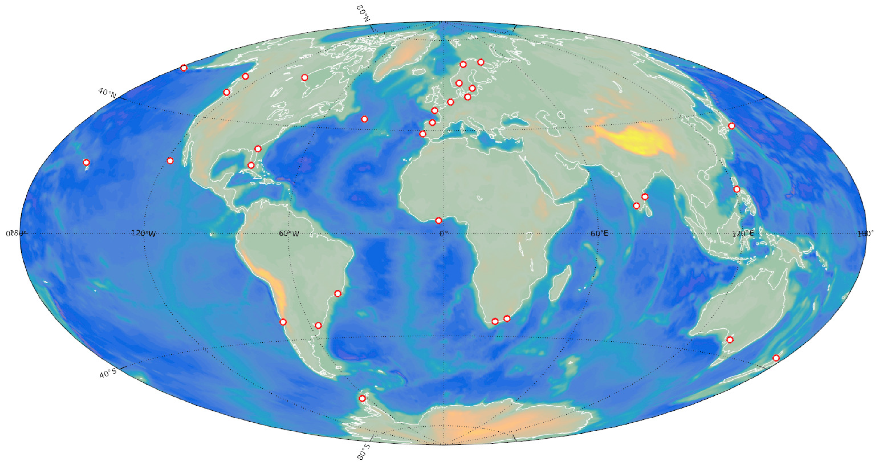
Figure 1. The full tide gauge database (1548 tide gauges of PSMSL series).
Jmse 10 01871 g001
Figure 2. Map showing the locations of tides gauges used to build the GSLTG series.
Jmse 10 01871 g002
Figure 3. Superposition of data series from the 31 tide gauges listed in Table 1.
Jmse 10 01871 g003
Figure 4. Fit of the 31 tide gauges. (a) Data points from the 31 tide gauges used in building GSLTG and their sinusoidal fit, with 8 sine waves. (b) The fit (black curve) of (a) with an enlarged ordinate scale.
Jmse 10 01871 g004
Figure 5. The first six most important components extracted from GSLTG. (a) First SSA component (1 yr) of the GSLTG data series of Figure 4b. (b) Second SSA component (∼90 yr) of the GSLTG data series. (c) Third SSA component (∼60 yr) of the GSLTG data series. (d) Fourth SSA component (∼80 yr) of the GSLTG data series. (e) Fifth SSA component (0.5 yr) of the GSLTG data series. (f) Sixth SSA component (∼20 yr) of the GSLTG data series.
Jmse 10 01871 g005
Figure 6. Superposition of the histogram of recent slopes of 1548 tide gauges with that of the MIDAS (GPS) data (from Hammond et al. [8]).
Jmse 10 01871 g006
Figure 7. Comparison of GPS and tide gauges slopes. (a). The locations of tide gauges and values of the local slope of sea-level change. Color code ranges from positive (red) to negative (blue). (b) The locations of GPS sites and the local changes (slopes) of vertical land movement (VLM) from the MIDAS database. Color code same as in (a).
Jmse 10 01871 g007
Figure 8. Global sea level GSLl curve from [27] in blue. Sum of first 6 components extracted by SSA, red curve.
Jmse 10 01871 g008
Figure 9. First six components extracted by SSA from GSLl data series. (a) The first SSA component (trend in red) superimposed on the GSLl data series. (b) Second SSA component (∼60 yr pseudo-period) of the GSLl data series. (c) Third SSA component (∼30 yr pseudo-period) of the GSLl data series. (d) Fourth SSA component (∼20 yr pseudo-period) of the GSLl data series. (e) Fifth SSA component (∼11 yr pseudo-period) of the GSLl data series. (f) Sixth SSA component (∼4 yr pseudo-period) of the GSLl data series.
Jmse 10 01871 g009
Figure 10. Global -sea level (GSLs) (blue curve). Sum of the first seven SSA components (red curve).
Jmse 10 01871 g010
Figure 11. First seven components extracted by SSA from GSL data series. First SSA component (trend) of the GSL data series of Figure 10. Second SSA component (1 yr) of the GSL data series. Third SSA component (0.5 yr) of the GSL data series. Fourth SSA component (3 yr) of the GSL data series. Fifth SSA component (15 yr) of the GSL data series. Sixth SSA component (1.5 yr) of the GSL data series. Seventh SSA component (6 yr) of the GSLs data series.
Jmse 10 01871 g011
Figure 12. Top left, the superposition of the trends of GSLTG (in black) and GP (in red). Middle left, the superposition of the trend of GSLTG (in black) and the first derivative of the trend of GP (in red). Bottom left, the ∼20 yr components of GP (red) and GSLTG (black). Top right and middle right (a zoom), the annual oscillations of GSLTG (black) and GP (red). Bottom right, the semi-annual cycles of GP (red) and GSLTG (black).
Jmse 10 01871 g012
Figure 13. Trends (top) and their derivatives (bottom) of the rotation pole (RP) coordinates m 1 (red) and m 2 (blue) compared with those for GSLTG (left; 1807–2020).
Jmse 10 01871 g013
Table 1. List of tide gauges selected in this study to build the GSLTG series.
Tide Gauge SiteLat ( )Lon ( )
Adak Sweeper Cove51.863−176.632
Argentine Islands−65.246−64.257
Auckland−36.843174.769
Brest48.3824.494
Churchill58.767−94.183
Chennai13.10080.300
Cochin9.96776.267
East-London−33.02727.932
Fernandina Beach30.672−81.465
Honolulu21.307−157.867
Ketchikan55.332−131.625
Key West24.555−81.806
Knysna−34.04923.046
Lisbon38.700−9.133
Marseille43.2795.354
Maasluis51.9184.25
Manila, S.harbor14.583120.967
Mera34.919139.825
Montevideo−34.900−56.250
Narvik68.42817.426
Oslo59.90910.735
Polyarny69.20033.483
Port Adelaide−34.780138.481
Rio de Janeiro−22.933−43.133
Swinoujscie53.91714.233
Takoradi4.885−1.745
Tofino49.150−125.917
Tuapse44.10039.067
Valparaiso−33.027−71.626
Visby57.63918.284
Xiamen24.450118.067
Table 2. Commensurate periods of the Jovian planets [41,51]. Periods of components extracted by SSA from sunspot series SSN, GSLl, GSLs and GSLTG are highlighted in red.
Jmse 10 01871 i001
Table 3. Ratios of SSA components of GP to GSLTG with the same periods (see text).
Sea Level (mm)Pressure (hPa)Ratio (hPa/mm)
Trend450.80.019
∼20–30 yr180.450.025
1 yr801.60.020
0.5 yr160.30.019
Publisher’s Note: MDPI stays neutral with regard to jurisdictional claims in published maps and institutional affiliations.

