Modeling of Thermodynamic Consolidation of Sea Ice Ridges Drifting in the Water with Changing Temperature

Abstract

Oceanographic and ice conditions in the region of Spitsbergen Bank in the Barents Sea were investigated in research cruises of the “Polarsyssel” in 2017–2019. Trajectories of ice drift were constructed using GPS data of the buoys deployed on the floes in the research cruises. The duration of the ice season in the region was analyzed using ice charts. The air temperature and wind velocities were analyzed using the data of meteorological stations on Bear Island and Hopen Island. Fieldwork on drifting ice showed the existence of thick consolidated floes with drafts up to 8 m, which were identified as completely consolidated sea ice ridges. The presence of such floes is dangerous for winter navigation along Spitsbergen Bank. A model of thermodynamic consolidation of ice ridges was formulated to investigate the thermodynamic evolution of ice ridges. The observed air and sea water temperatures were used in the boundary conditions on top and bottom surfaces of sea ice rubble. It was shown that the regular interaction of sea ice rubble with Atlantic and Arctic waters in the region of Spitsbergen Bank leads to almost complete consolidation of the ice rubble with an initial macro-porosity 0.2 for 150 days.

1. Introduction

Ice ridges are formed in sea ice due to the compressive failure of floe edges at their contact lines and consequent pushing of ice chunks in the water below the ice and on the ice surface. Usually, ice ridges are extended along the floe edges, but in cases of relatively small diameters of interacting floes, ridged ice can occupy regions of arbitrary shapes. The vertical dimension of ice ridge keels is greater than the vertical dimension of their sails in three to five times [1]. The length of ice ridges can reach several kilometers and greater [2]. Although vertical sizes of ice ridges exceed the thickness of level ice several times, the initial strength of ice rubble filling ridge keels is not high, because submerged ice chunks are not frozen with each other. The disposition of submerged ice chunks is characterized by the macro-porosity of ice rubble. The macro-porosity equals the ratio of the volume of sea water trapped inside ice rubble to the total volume of the rubble. Field investigations showed the ice rubble macro-porosity changing from 0.1 to 0.7 [3] (p. 206). The most frequent values of the macro-porosity are in the range from 0.2 to 0.3. The structure of submerged ice chunks is characterized by their microporosity, which is equal to the ratio of the volume of gas and liquid brine inside a chunk to the chunk volume [4].

Thermodynamic effects influence the formation of freeze bonds between submerged ice chunks, increasing the ice ridge strength. The thermodynamic consolidation of ice rubble occurs due to atmosphere cooling [5,6], the release of cold reserves from submerged ice chunks [7,8], and the penetration of fresher water inside ridge keels [9]. The shape of consolidated rubble inside ice ridge keels is similar a layer. Therefore, it is named the consolidated layer (CL). The ice rubble below the CL is not consolidated and further referred to as unconsolidated rubble (UR).

A simple model of thermodynamic consolidation of floating ice ruble due to atmosphere cooling based on the Stefan equation and assumption that UR is at the freezing point of sea water predicted the thickness of the consolidated layer as greater the level ice thickness by 1.6–2 times [10]. The maximal thickness of level sea ice in the Barents Sea is below 1 m. In the East-Siberian Sea, the Chukchi Sea and Beaufort Sea maximal thickness of level sea ice reaches 2–2.5 m. It means that the maximal thickness of consolidated layers in the Barents Sea is below 2 m, and in the East Arctic, it is below 4–5 m. At the same time, it is known that multiyear ice ridges with drafts greater than 5 m can be completely consolidated [11]. Høyland et al. [12], Strub-Klein et al. [13], and Shestov et al. [14] discovered that the second-year ice ridges in the Fram Strait are also completely consolidated. Field investigations of drift ice along Spitsbergen Bank in April 2017–2019 showed the existence of completely consolidated ice ridges with drafts up to 8 m [3].

Field measurements of the macro-porosity of ice ridges are performed by drilling. Completely consolidated ice ridges are those where the auger did not drop suddenly on some significant distance, which is recognized by the driller as a cave filled by water during the drilling of the ridge keel. Small caves of 10 cm in depth and smaller are not well-recognized by mechanical drilling. It influences the practical definition of completely consolidated ridges. For example, a macro-porosity of 0.1 means that an ice rubble of 10 m thickness includes 10 caves of 10 cm in depth that are not recognized by the drilling. Therefore, ridge keels with a macro-porosity of 0.1 and smaller can be considered as almost completely consolidated formations. The value 0.1 is also close to the microporosity of submerged ice chunks at −2 °C and salinity 5 ppt [4].

Ocean heat flux influences the melting of ridge keels and penetration of melt water inside them. Sea water trapped inside ridge keels is at the freezing point. The mixing of fresher and warmer melt water with saltier and colder sea water trapped inside keels leads to the formation of new ice. It influences the decreasing of the macro-porosity of ice ridges. The mathematical model of this process was formulated and investigated using the assumption that the temperature of UR and sea water inside UR equals the freezing point of sea water below UR [3]. The freezing point was assumed given. A set of model equations consisted of two Stefan equations and a salt balance equation. Stefan equations describe the growth of CL due to the cooling from atmosphere and the melting of UR from below due to the ocean heat flux. The salt balance equation describes the evolution of the macro-porosity of UR under the influence of salt fluxes at the boundaries. Numerical simulations were performed to estimate the time to complete the consolidation of ice rubble with an initial porosity from 0.2 to 0.3. It was shown that decreasing the ocean heat flux and increasing the initial macro-porosity influence increased the time of consolidation. The time of consolidation of ice rubble with an initial draft of 10 m and an initial macro-porosity of 0.2 was estimated about 200 days with an ocean heat flux of 20 W/m².

In the region of Spitsbergen Bank, Arctic waters coming from the northeast are mixed with Atlantic waters going around the bank to the north–east and to the northwest. This branch of Atlantic waters follows the west coast of Spitsbergen and penetrates inro the Barents Sea from the north between Svalbard and Franz Josef Land [15]. In the ice season, Arctic waters are at the freezing point, while Atlantic waters are above the freezing point. The salinity of Arctic waters is smaller than the salinity of Atlantic waters. Sea ice in the region of Spitsbergen Bank can drift by wind drag in the regions with colder and fresher Arctic waters and warmer and saltier Atlantic waters. Changes of water temperature below ice rubble influences changes of the ocean heat flux and the ice rubble temperature. The above-described model of thermodynamic evolution of ice ridges should be modified according to the oceanographic conditions along Spitsbergen Bank.

In the present paper, we describe the oceanographic conditions along Spitsbergen Bank, formulate a new model of thermodynamic evolution of ice rubble, and describe the results of numerical simulations of thermodynamic consolidation and melting of ice rubble drifting in the region of Spitsbergen Bank. Ice conditions along Spitsbergen Bank are discussed in Section 2 of the paper. Sea water characteristics and weather conditions are described in Section 3, Section 4 and Section 5. A model of thermodynamic consolidation and melting of ice ridges is formulated in Section 6. The results of numerical simulations are described in Section 7. Main achievements of the work are formulated and discussed in Conclusions.

2. Ice Conditions along Spitsbergen Bank

The shallow region of the Barents Sea with depths smaller than 100 m extending between Bear Island and Hopen Island is called Spitsbergen Bank (Figure 1a). The double black line in Figure 1a shows the location of the Polar Front between colder Arctic waters and warmer Antarctic waters. The red and blue lines show the directions of Atlantic and Arctic water currents, and the Tidal Front is shown by the blue triangles. The inflow of Artic water in shallow Spitsbergen Bank with depths below 50 m influences the extended ice season in comparison to the other regions of the Barents Sea located at the same latitudes. Isolines of the sea ice concentration in Figure 1b show that the ice edge along Spitsbergen Bank near Bear Island takes the most southern position in the Barents Sea.

Duration of the ice season along Spitsbergen Bank was estimated using ice maps downloaded from https://cryo.met.no (assessed on 22 August 2022). White bands and dots in Figure 2 show the days from 1998 to 2022 when the ice edge crossed the latitude 75° N to the north of Bear Island (Figure 1). The data for 2011 are shown by a solid white band in Figure 2, since the web resource did not provide ice maps for this year. The first appearance of sea ice at 75° N after the summer seasons was registered at the end of December, and the last observation of ice appearance at 75° N was registered in June. Most frequently, sea ice was found at 75° N in March and April. 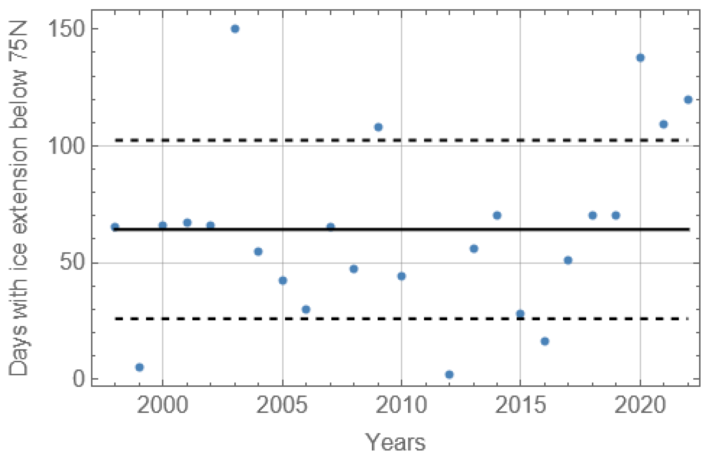Figure 3 shows annual numbers of days per year (AD75) when the ice edge crossed the 75° N latitude to the north of Bear Island since 1998. AD75 reached the maximum of 150 days in 2003, and it was equal to 138 days in 2020. Minimal values of AD75 reached 2 days in 2012 and 5 days in 1999. The mean value of AD75 shown by a solid black line in Figure 3 equals 60, and the standard deviation is 36.6 days.

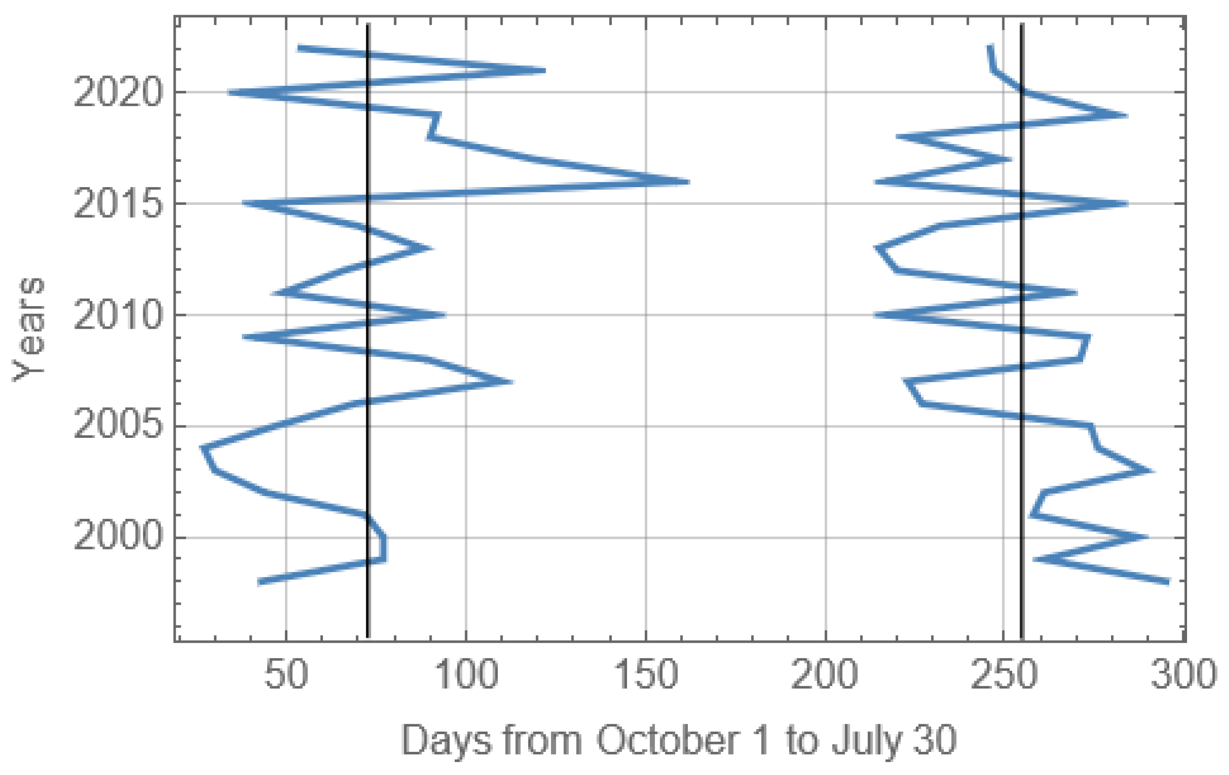
Broken lines in Figure 4 show the dates when sea ice was observed near Hopen Island in the first time (left line) and in the last time (right line) during ice seasons in 1998–2022. Straight lines show the mean dates of the beginning (December 11) and the end (June 11) of the ice seasons. It is possible to see a shortening of ice seasons from 1998 to 2017 and an extension of ice seasons after 2017. The mean duration of the ice seasons near Hopen Island (ADH) is 181 days. Standard deviations of the beginnings and the ends of the ice seasons are, respectively, 32 days and 25 days. Thus, ADH is three times greater than AD75.

Sea ice was observed and investigated during the research cruises of the “Polarsyssel” in the region of Spitsbergen Bank on 22–30 April 2017, 24–30 April 2018, and 23–29 April 2019. Trajectories of the “Polarsyssel” surveys are shown in Figure 5. The bathymetry map is constructed using Wolfram Mathematica GeoElevationData software. The field investigations were performed in ice-covered regions of the bank. The extension of sea ice along Spitsbergen Bank on 27 April in 2017, 27 April in 2018, and 26 April in 2019 is shown in Figure 6 (https://cryo.met.no, accessed on 20 November 2022). The shapes of areas covered by sea ice are very similar in 2017 and 2018 and different from the shape of the ice-covered area in 2019. It is explained by dominant winds in northern and southern directions in April of 2017 and 2018 and dominant wind from the west in the end of April 2019 (https://earth.nullschool.net, accessed on 20 November 2022).

The areas covered by sea ice in the region of Spitsbergen Bank in 2017 and 2018 are associated with sea depths smaller than 100 m. Depending on the weather conditions, the ice edge may extend to Bear Island or be located north of the island. Winds from the north influence ice drift to Spitsbergen Bank from the Olga Basin. Winds from the south may displace sea ice from the bank to the Store Fjord and Hopen Island, where the seawater temperature is near the freezing point. Winds from the west and the east displace ice in the regions of warm Atlantic currents, where the oceanic heat flux to the ice bottom influences ice melt. The latitude 75° N can be considered as a boundary characterizing the southern location of the ice edge along Spitsbergen Bank.

Drift ice observed along Spitsbergen Bank during the cruises consisted of relatively big areas with slushy ice, sea ice floes with a thickness of 30–40 cm, and diameters 10–100 m; consolidated sea ice floes with mean drafts 4–6 m and diameters 20–50 m; and bergy bits [16]. In 2019, fieldwork was performed on the consolidated floe with draft up to 9 m [3]. Thick consolidated floes were found in each of the cruises. Their occurrences were not rare events. Nevertheless, the number of consolidated floes was smaller than the number of floes with 30–40 cm in thickness. 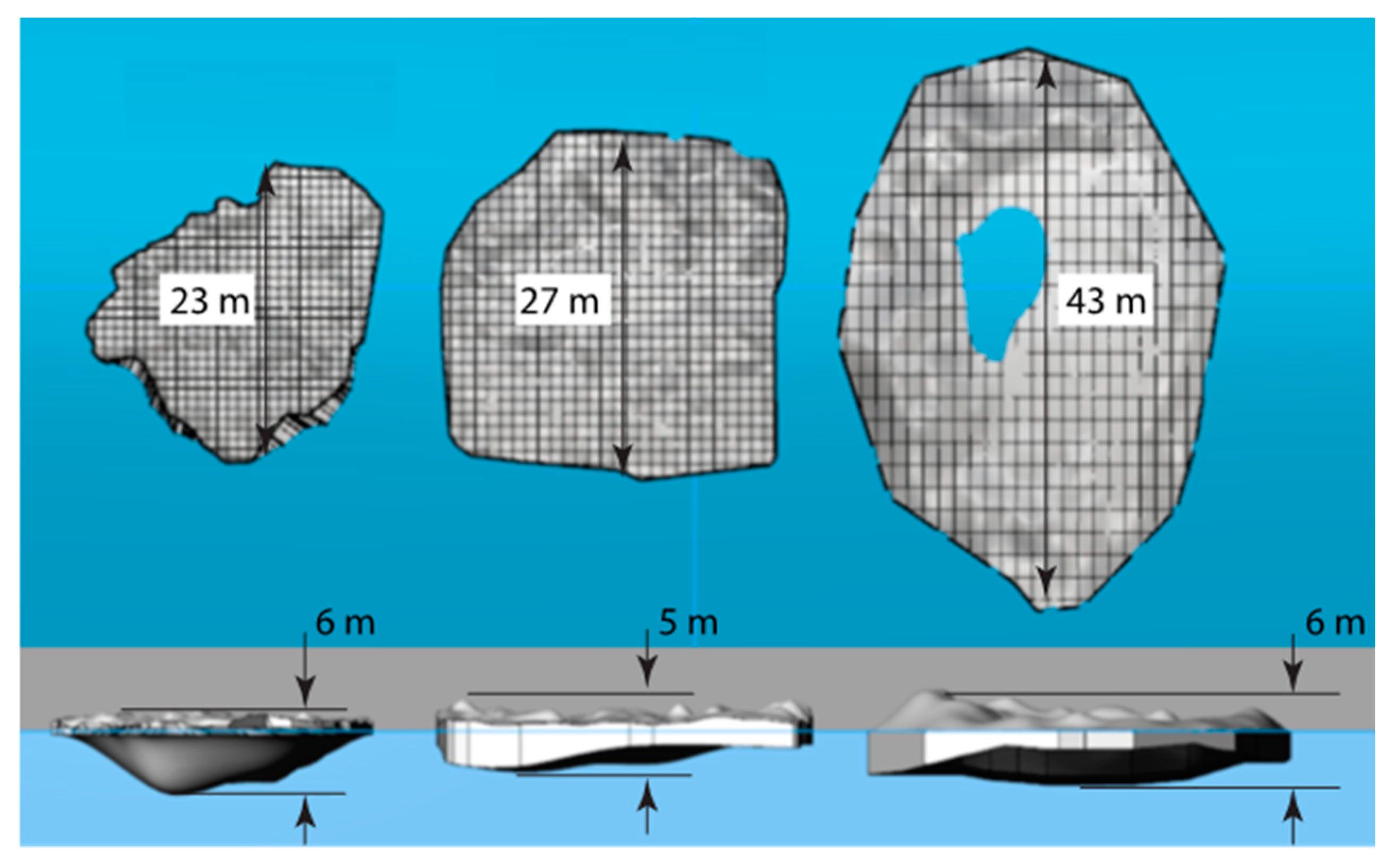Laser scanning and drilling studies were performed to investigate the structure and shape of the thick floes [16]. Examples of computational models of three floes investigated in 2017 and 2018 are shown in Figure 7. One can see that all floes have smoothed shapes and maximal thickness of 5–6 m. Thick consolidated floes consisting of the first-year sea ice were recognized as completely consolidated ice ridges [3]. We did not observe strong interactions of floes along Spitsbergen Bank and assumed that the observed consolidated ice ridges formed in some other places.

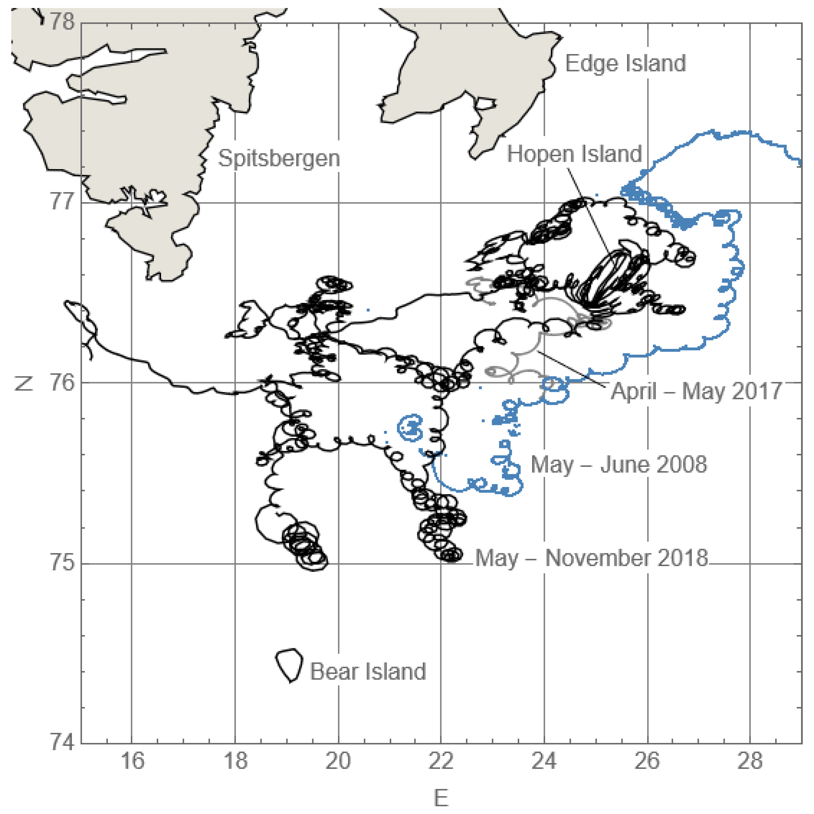
Figure 8 shows trajectories of three drifting buoys (Oceanetic Measurements Ltd., North Saanich, BC, Canada) deployed on sea ice along Spitsbergen Bank in 2008, 2017, and 2018. After the ice melt, the buoys survived and transmitted the data as trackers of surface currents. The GPS data were transmitted with 15-min sampling intervals via Iridium. The buoy trajectories consist of many loops passed by the buoys in a clockwise direction [17,18]. The clockwise motion of water and sea ice with a semidiurnal period are forced in the region by the semidiurnal tide [19]. The motion of drifting ice along Spitsbergen Bank can be considered as a free drift with significant shear deformations [20]. The shear deformations are explained by the actions of strong tidal currents in combination with wind and swell drags. Depending on the wind conditions, some of the buoys deployed along Spitsbergen Bank drifted in the region over several months (see the trajectory of the buoy deployed in 2018 in Figure 8), while other buoys left the region in a few weeks [20].

3. Sea Water Salinity and Temperature

Cold Arctic water transported by the East Spitsbergen current from the north interacts with warm Atlantic water in the Barents Sea [21]. The boundary zone between these waters shown in Figure 1a by a double black line is called the Polar Front [22]. Atlantic water has a higher salinity and density than Arctic water. The temperature of an “ideal” Arctic water is close to the freezing point (~−1.9 °C), and the salinity is below 34.5 PSU. The salinity of an “ideal” Atlantic water is around 35° PSU, and the temperature is above 0 °C [23]. Therefore, Atlantic water tends to occupy deeper ocean layers when it meets with colder and fresher Arctic water. One branch of Atlantic water penetrates the Barents Sea through the Barents Opening, and the other branch follows the west coast of Spitsbergen and penetrates the Barents Sea from the north between Svalbard and Franz Josef Land [15]. Polar Front water is saltier than Arctic water but colder than Atlantic water [24,25].

Measurements of vertical profiles of sea water temperature and salinity (CTD profiling) were performed 18 April–18 May 2008, along a 125-km transect extended between 250 m and 100 m isobaths in the range 23°–27° E and 75.5°–76.2° N [24] and on 9–10 August 2009 along a 200-km transect crossing the Spitsbergen Bank in the range 20°–25° E and 75°–76° N [25]. The shallow part of Spitsbergen Bank to the north of Bear Island is occupied by well-mixed Spitsbergen Bank water with a lower salinity than Polar Front water. Mixing is caused by strong tidal currents [26,27], wind forcing, and convection [24,28]. Wind action during cold weather may influence the overcooling of the surface water layer and the formation of frazil ice [29]. Consecutive convection replaces cold and saline water at the surface with slightly less saline and cold water from below. The processes of overcooling and frazil ice formations were observed and investigated in Storfjorden, Svalbard, in April 2006 [29].

The temperature and salinity measurements were performed by CTD profiling with SBE-19 in April 2017–2019 from drifting floes and from the board of the “Polarsyssel”. Locations, dates, and times of CTD profiling in 2017 and 2018 are shown in Figure 5 by points 1–7, and the times of the measurements are specified in

Table 1. Dates and time (UTC) of CTD profiling in April of 2017 and 2018.

Locations	1	2	3	4	5	6	7	8	9
Days and time, April 2017	24 11:30	25 11:26	26 22:17	27 03:17	27 07:08	27 10:37	28 10:32
Days and time, April 2018	26 07:38	26 08:44	26 12:10	27 11:02	27 15:10	27 18:40	27 20:20	27 21:05	28 08:43

. Vertical profiles of temperature and salinity measured in 2017 and 2018 are shown, respectively, in Figure 9a–d. In 2017, the CTD profiles in points 1 and 2 were measured from the floe, and the CTD profiles in points 3–7 were measured from the board of the “Polarsyssel” when she was moored and drifted together with a floe on 24–26 April near the point (23° E, 76.5° N). Then, the vessel crossed Spitsbergen Bank for visual observations of the ice conditions and CTD profiling in points 3–6 and returned to point 7 located near points 1 and 2 (Figure 5). The CTD profiles 1, 2, and 7 were performed almost in the same place near the tip of Store Fjord Trough but at different times. They demonstrate the strong spatial and temporal variability of the water characteristics in this place. The water characteristics at depths below 70 m are close to the characteristics of the “ideal” Atlantic water, and the water characteristics above this level are close to the Polar Front water, which is saltier than Arctic water but colder than Atlantic water [23,24,25].

The CTD profiles 3–6 were performed in the regions with depths shallower than 60 m. The water temperature was below −1.5 °C, and the water salinity was higher than 34.65 PSU in points 3 and 4. According to [24,25], the water masses in these locations are interpreted as the Polar Front water. In point 5, the water temperature was around −1.85 °C, and the salinity was around 34.68 PSU at the depths exceeding 10 m. At smaller depths, the salinity dropped to 34.42 PSU. The characteristics of the surface layer in point 6 were close to the “ideal” Arctic water. In point 6, the water temperature at depths smaller than 30 m varied between −1.5 °C and −1.0 °C, while the salinity decreased with the depth. It influenced the unstable stratification, causing water mixing. The water layer below 30 m can be interpreted as the Polar Front water. The surface layer salinity was close to the salinity of the “ideal” Atlantic water, but the water temperature was lower.

In 2018, CTD profiles 1–9 were performed from the ice floes or from the board of the “Polarsyssel” moored to the floes. Profiles 1–5 and 6–9 were recorded when the vessel was moored to the middle and right floes shown in Figure 7, respectively. Profiles 1–3 were performed in the depth range 40–50 m, profiles 4–6 were performed in the depth range 60–80 m, and profiles 7–9 were performed in the depth range 20–40 m in the shallowest part of Spitsbergen Bank. The salinity above 34.8 PSU supports to consider this water as cooled Atlantic water. Profiles 4–6 correspond to the Polar Front water. The salinity is approximately 34.5 PSU, and the temperature is around −1.8 °C on profiles 7–9. Their characteristics are close to the “ideal” Arctic water.

Figure 10 shows temperature-salinity diagrams based on CTD profiles measured in 2017 and 2018 in the shallowest regions of Spitsbergen Bank. Profiles 1–3 in 2018 show the temperature near the freezing point, and profile 2 indicates overcooling of the water column from 15 m to 40 m in depth. The overcooling may happen due to water mixing caused by tidal currents and strong wind in cold weather [29]. The overcooling was confirmed by large areas of slush on the sea surface observed during the fieldwork in 2018.

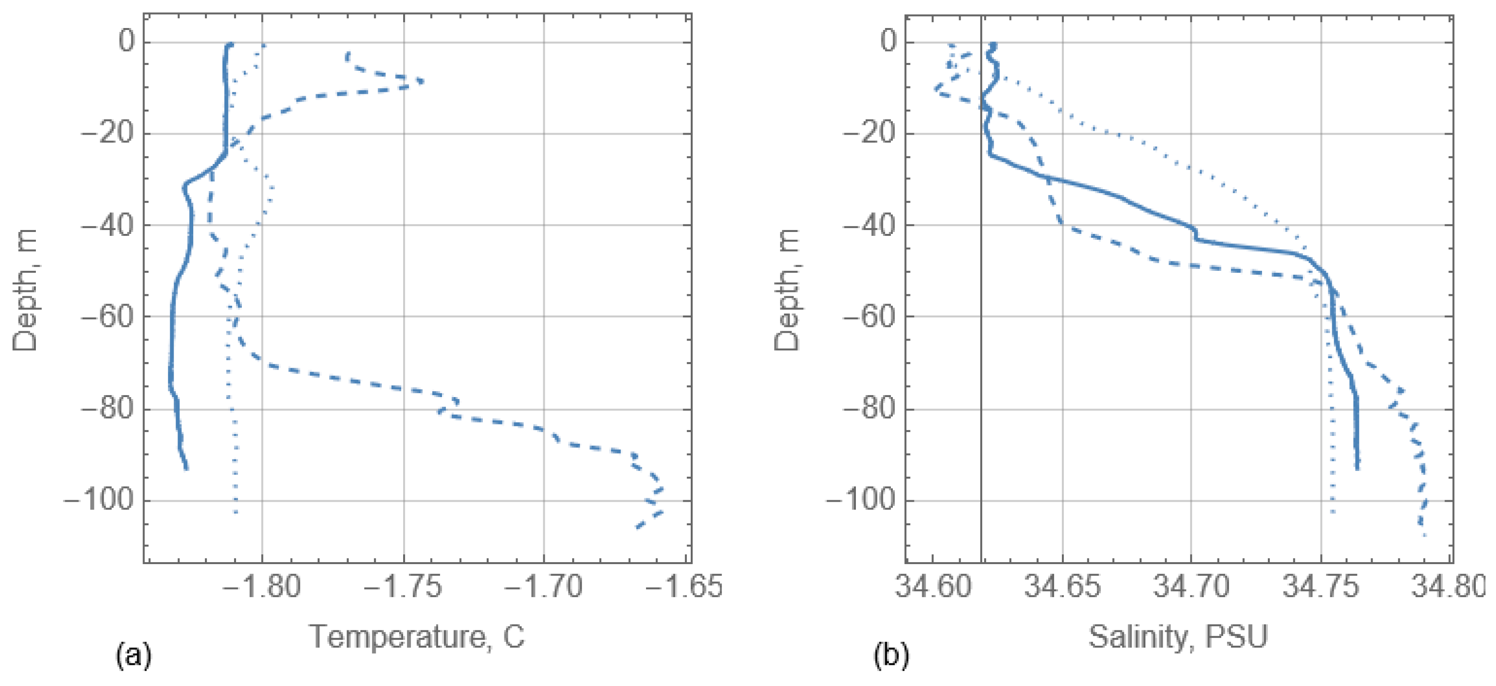
In 25–27 April 2019, all CTD profiles were performed from the “Polarsyssel” with a cast interval of one hour. The measurements were located over the bottom slope of Hopen Island at a distance 30 km from the island over a depth of 98–110 m (Figure 5). The ship drifted near consolidated floe with 9 m of draft, where the fieldwork was performed by moto-boats. Examples of temperature and salinity profiles from 25 to 27 April 2019 are shown in Figure 11. We note strong time variations in the vertical profiles associated with the internal waves of the semidiurnal period [30]. The water temperature within the water column changed between −1.83 °C and −1.65 °C, and the salinity changed between 34.6 PSU and 34.8 PSU. These characteristics indicates Polar Front water [31].

4. Heat Flux from Ocean to Sea Ice

Point measurements of the water velocities below the drift ice were performed in 2017 and 2019 using the Acoustic Doppler Velocimeter (ADV) SonTek (Ocean Probe 5 MHz) with 10 Hz sampling frequency. Temperature and pressure recorder SBE-39Plus was mounted together with the ADV and recorded the data with sampling frequency 2 Hz. In 2017 and 2019, the sensors were mounted in down-looking positions, respectively, on the sides of drifting floes. In 2018, the Acoustic Doppler Current Profiler (ADCP) RDI Workhorse 1228 kHz was deployed on the side of a floe also in the down-looking position. It was programmed to the sampling frequency of 5 Hz. The bin size was 25 cm, and the first bin range was 61 cm. The recorder SBE-39Plus was mounted on the side of the ADCP and recorded the temperature data with a sampling frequency 2 Hz. The deployment dates are shown in

Table 2. Dates and time (UTC) of water velocity measurements with the Acoustic Doppler Velocimeter (ADV) and the Acoustic Doppler Current Profiler (ADCP) in April 2017–2019.

Year	2017, ADV	2018, ADCP	2019, ADV
Days and time	24,14:54–25, 20:41	26,15:05–27, 07:58	25,18:22–27, 08:17
HF, W/m2	12,7; 19.5; 91.1	15.2	27.3

. In 2017, the measurements were performed near points 1 and 2, and in 2018, the measurements were performed near points 1–3 (Figure 3). In 2019, the measurements were performed near the “Polarsyssel” track shown in Figure 5. All records listed in Table 2 were performed when the “Polarsyssel” was disconnected from the floes and drifted at a distance greater than 300 m from them. In 2017, the ADV record within the time interval specified in Table 2 was performed in three stages.

The vertical ocean heat flux to the drift ice was calculated with the formula

$$Q_w={\rho }_{sw}c\langle {v^{\prime }}_z{T}^{\prime }\rangle ,$$

(1)

where ${\rho }_{sw}$= 1028 kg/m³ is the mean sea water density, $c=4.19$ kJ/kg·C is the specific heat capacity of water, ${v^{\prime }}_z$ is the fluctuation of vertical water velocity, and $T^{\prime }$ is the fluctuation of the water temperature. Symbol 〈 〉 means averaging over the specific interval of the measurements, which was programmed to 270 s within the burst interval of 300 s in 2017 and 600 s within the burst interval of 700 s in 2019. The fluctuations were calculated by the formula

$${v^{\prime }}_z=v_z-\langle v_z\rangle , T^{\prime }=T-\langle T\rangle ,$$

(2)

where $v_z$ and $T$ are measured values of the water velocity and temperature.

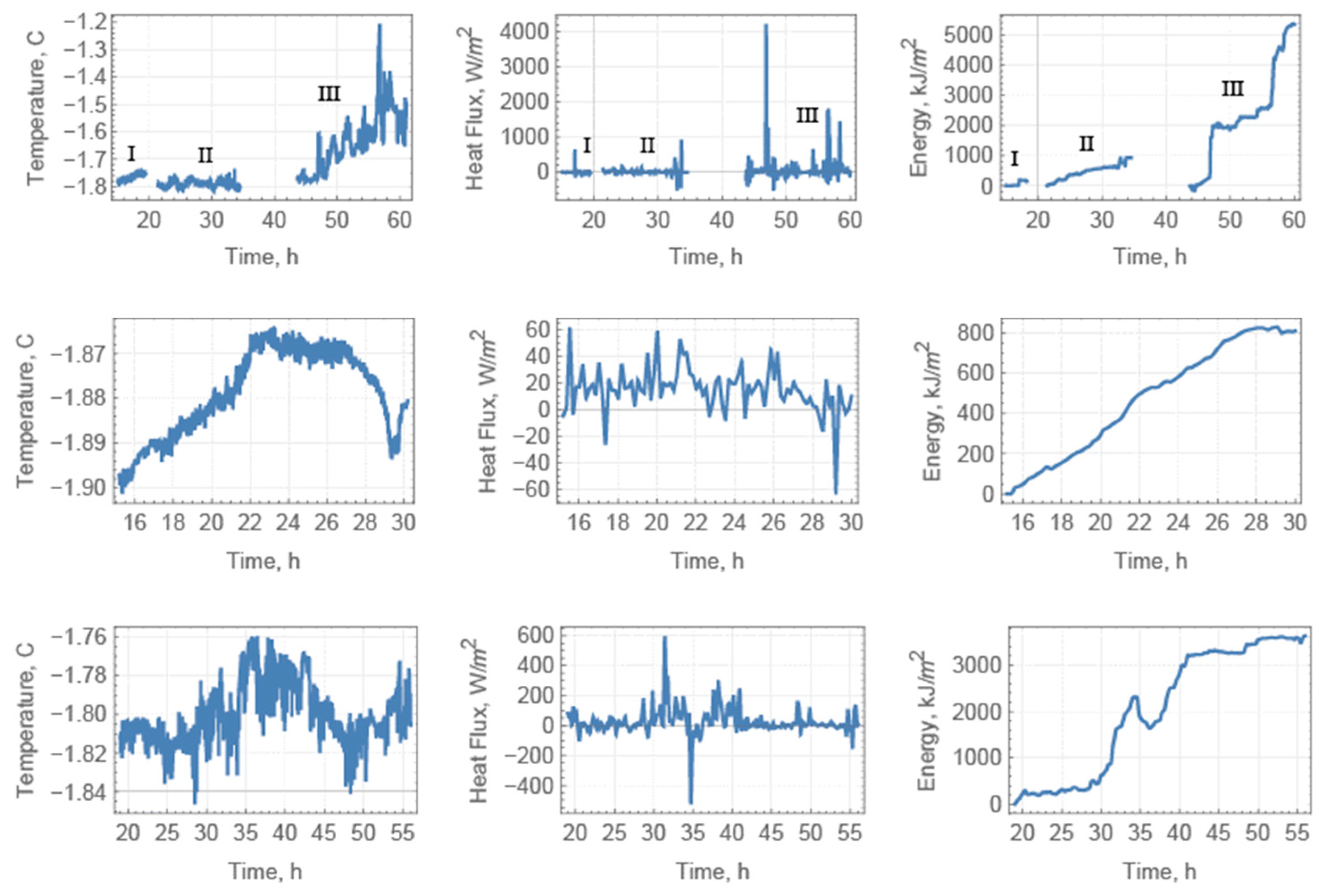
Figure 12 shows the recorded temperature below the ice (left panel), calculated ocean heat flux (middle panel), and cumulative heat flux (energy) versus time. The mean heat fluxes during three stages of measurements in 2017 were estimated as 12.7 W/m², 19.5 W/m², and 91.1 W/m². The increase in the heat flux on the third stage is explained by the increase of the water temperature from −1.8 °C to −1.2 °C (Figure 11, left graph in the top panel). In 2018 and 2019, the mean heat fluxes were 15.2 W/m² and 27.3 W/m², respectively.

5. Weather Conditions

Wind rise constructed with weather data from the meteorological station on Bear Island is shown in Figure 13 for the period from October 2018 to June 2019. Wind rise constructed for the same period in 2016–2017 and 2017–2018 was very similar. Dominant winds from north–Northeast influence ice drift to Bear Island. The probability of other wind directions is lower than 5%, and it is distributed uniformly over the azimuthal angle. Highest wind speed below 20 m/s is also distributed uniformly over the azimuthal angle. Wind drags supports the general direction of ice drift to Spitsbergen Bank from the northeast. At the same time, winds of other directions influence regular displacements of ice from Spitsbergen Bank in different directions.

Figure 14 shows the air temperature measured on the meteorological stations on Bear Island and Hopen Island. Although the air temperature on Hopen Island is lower than on Bear Island, the temperature changes over 280 days starting on 1 October are very similar. Lowest air temperatures below −15 °C were recorded in March and April. Stable negative air temperature was recorded in the period from December to May. Further, for the modeling of thermodynamic processes in ice ridges, we used the mean air temperature calculated with the data shown in Figure 14.

6. A Model of Thermodynamic Consolidation of Ice Ridges

6.1. General Assumptions

For the construction of a mathematical model describing the thermodynamic consolidation of ice ridges the following assumptions about the structure of their keels are made. The ridge keel consists of a consolidated layer (CL) in the upper part of the keel and unconsolidated rubble (UR) below CL (Figure 15a). Volumetric portion of water in UR is characterized by the macro-porosity $p$. Macro-porosity of CL equals zero. The thicknesses of CL and UR are denoted as $h_{cl}$ and $h_{ur}$, respectively. Thermal inertia is ignored inside CL, and the temperature profile in CL changes linearly from the surface temperature $T_s$ at $z=0$ to the bottom temperature $T_{ur}$ at $z=-h_{cl}$ (Figure 15a). According to the thermodynamic equilibrium, the UR temperature $T_{ur}$ equals the freezing point $T_f\left({\sigma }_{ur}\right)$ of seawater inside UR, where ${\sigma }_{ur}$ is the water salinity. The salinity of sea water inside UR and the salinity of brine inside submerged ice chunks inside UR are the same. The temperature $T_{ur}$ and water salinity ${\sigma }_{ur}$ depend on time but are constant over the UR thickness (Figure 15a).

Simplified formula describing the dependence of the freezing point from the salinity was given in [32]:

$${\sigma }_{ur}=\alpha T_{ur}, \alpha =-0.0182 {\mathrm{C}}^{-1}.$$

(3)

Sea water temperature ($T_{sw}$) and salinity (${\sigma }_{sw}$) below UR can be different from $T_{ur}$ and ${\sigma }_{ur}$. It leads to a difference of the densities of sea water trapped inside UR (${\rho }_{ur}$) and sea water below UR (${\rho }_{sw}$). Further, we assume neutral or stable stratification of sea water. The inequality:

$${\rho }_{ur}\le {\rho }_{sw},$$

(4)

corresponds to this assumption.

Sea water salinity changes in the range of 33–35 PSU in the Barents Sea, while sea ice salinity is usually smaller than 15 PSU. Variations of sea water temperature and salinity below drift ice caused by the penetration of Atlantic waters in ice-covered regions of the Barents Sea are, respectively, of about 1 °C and 1 PSU. Seawater temperature below drift ice is changed in the range from the freezing point to about 1 °C above the freezing point $T_f\left({\sigma }_{sw}\right)$. Seawater density in a proximity of the freezing point can be calculated with the formula

$${\rho }_{sw}\left({\sigma }_{sw},T\right)={\rho }_{sw}\left({\sigma }_{sw},T_f\left({\sigma }_{sw}\right)\right)+{\frac{\partial {\rho }_{sw}\left({\sigma }_{sw},T\right)}{\partial T}|}_{T=T_f\left({\sigma }_{sw}\right)}\left(T-T_f\left({\sigma }_{sw}\right)\right).$$

(5)

where ${\rho }_{sw}$ is the sea water density at atmosphere pressure. The melting of ice rubble from below may lead to the penetration of melt water with low salinity inside UR. Water freezing at the bottom of CL leads to the formation of saline water near the surface of UR. Variations of sea water salinity inside UR up to 25 PSU influence the water density gradients, leading to water mixing inside UR.

From the sea water density derived in [33] and freezing point formula derived in [34], it follows:

$$\begin{gathered} \left|{\rho }_{sw}\left({\sigma }_{sw},T_f\left({\sigma }_{sw}\right)+1°\mathrm{C}\right)-{\rho }_{sw}\left({\sigma }_{sw},T_f\left({\sigma }_{sw}\right)\right)\right|\le 0.03 \mathrm{kg}/{\mathrm{m}}^3, {\sigma }_{sw}\in \left(10,35\right) \\ {\rho }_{sw}\left(35 \mathrm{PSU},T_f\left(35 \mathrm{PSU}\right)\right)-{\rho }_{sw}\left(10 \mathrm{PSU},T_f\left(10 \mathrm{PSU}\right)\right)\approx 20.25 \mathrm{kg}/{\mathrm{m}}^3. \end{gathered}$$

(6)

Therefore, seawater salinity has a dominant influence on seawater density inside and in the proximity of UR. Based on these estimates, we replace inequality (4) with

$${\sigma }_{ur}\le {\sigma }_{sw}.$$

(7)

The sea ice density, the specific heat capacity $c_{si}$, and the latent heat $L_{si}$ of sea ice formation are determined by the formulas [32]

$${\rho }_{si}=\frac{\alpha {\rho }_{ur}{\rho }_i{T}_{ur}}{{\sigma }_{si}\left({\rho }_i-{\rho }_{ur}\right)+\alpha {\rho }_{ur}{T}_{ur}\left(1-{\sigma }_{si}\right)}, c_{si}=-\frac{{\sigma }_{si}{L}_i}{\alpha T_{ur}^2}+\frac{{\sigma }_{si}\left(c_w-c_i\right)}{\alpha T_{ur}}+c_i, L_{si}=\left(1-{\sigma }_{si}-\frac{{\sigma }_{si}}{\alpha T_{ur}}\right)L_i,$$

(8)

where $c_w=4.18$ J/(kg C) and $c_i=2.14$ J/(kg C) are the specific heat capacities of water and pure ice, $L_i=334$ kJ/kg is the latent heat of pure ice formation, and ${\rho }_i=917$ kg/m³ and ${\rho }_{ur}$ are the densities of pure ice and sea water trapped in UR. In the simulations, sea water densities ${\rho }_{ur}$ and ${\rho }_{sw}$ are calculated with standard formulas [33].

6.2. Model Equations

The heat $Q_s$ flux from the ice into the air influences water freezing between submerged ice chunks of UR, leading to the formation of CL. The CL thickness $h_{cl}$ increases in time according to the heat flux $Q_{cl}$ at the CL bottom. The thickness of CL is calculated from the Stefan equation

$${\rho }_{si}p{L}_{si}\frac{d{h}_{cl}}{dt}=Q_{cl}us\left(T_{ur}-T_s\right),$$

(9)

where $T_s$ is the temperature at the surface of CL. The unit step function $us\left(x\right)=0$ by $x<0$, and $us\left(x\right)=1$ by $x\ge 0$. The unit step function is used to exclude the melting of CL at the bottom when the surface temperature is higher than the freezing point. The heat flux is proportional to the vertical temperature gradient in CL

$$Q_{cl}=k_{si}\frac{\Delta T}{h_{cl}},$$

(10)

where $\Delta T=T_{ur}-T_s$, and $k_{si}=2.22$ W/(m C) is the thermal conductivity of sea ice. Formula (10) estimates the heat flux using assumption on linear dependence of the CL temperature $T_{cl}$ from the vertical coordinate $z$ (Figure 14a). It means that $Q_s=Q_{cl}$ and corresponds to the field observations [6,9].

The ice rubble melts from below due to the ocean heat flux, and melt water penetrates inside the UR. As a result, the ice rubble draft $h_r$ and macro-porosity $p$ decrease. The Stefan boundary condition at the bottom of UR is written as follows

$${\rho }_{si}\left(1-p\right)L_{si}\frac{d{h}_r}{dt}=-Q_{w}us\left(T_{sw}-T_{ur}\right),$$

(11)

where $Q_w$ is the heat flux from ocean (Figure 15b). The unit step function is used to exclude increasing $h_r$ when the sea water temperature is lower the temperature of UR. In this case, the vertical heat flux influences a decrease of the UR temperature, but the draft of UR does not change.

The ocean heat flux is determined by the formula [35]

$$Q_w={\rho }_{sw}{c}_{sw}{u}_{*}{\mathsf{\Phi }}_T^{-1}\left(T_{sw}-T_{ur}\right),$$

(12)

where $u_{*}$ is the turbulent velocity scale, and ${\mathsf{\Phi }}_T\approx 200$ is the Stanton number [36]. From Formula (12), it follows that $us\left(T_{sw}-T_{ur}\right)=1$ only when $Q_w\ge 0$.

The heat balance of UR is described by the thermal energy equation integrated over the UR thickness [37]

$$\begin{gathered} h_{ur}\left(\left(1-p\right){\rho }_{si}{c}_{si}+p{\rho }_{ur}{c}_{sw}\right)\frac{d{T}_{ur}}{dt}+{\rho }_{si}{h}_{ur}{L}_{si}\frac{dp}{dt}= \\ =-(p us\left(T_s-T_{ur}\right)+\left(1-p\right))Q_{cl}+\left(\left(1-p\right)us\left(T_{ur}-T_{sw}\right)+p\right)Q_w, \end{gathered}$$

(13)

where $h_{ur}=h_r-h_{cl}$ is the thickness of UR.

Mass of salts in a vertical column of UR with the horizontal cross-section of the unit area equals

$$S_{ur}=h_{ur}\left[{\sigma }_{ur}{\rho }_{ur}p+{\sigma }_{si}{\rho }_{si}\left(1-p\right)\right].$$

(14)

Salt fluxes at the bottom of CL and at the bottom of UR influence the water salinity inside UR and may cause the formation of new ice or melting of existing ice inside UR. The salt flux at the bottom of CL consists of two parts. The first part ($F_{sw,cl}>0$) describes salt expulsion into the water below CL due to the growth of CL:

$$F_{sw,cl}=p\left({\sigma }_{ur}{\rho }_{ur}-{\sigma }_{si}{\rho }_{si}\right)\frac{d{h}_{cl}}{dt}.$$

(15)

The second part describes salt deflux ($F_{si,cl}<0$) from UR due to the incorporation of ice chunks into CL:

$$F_{si,cl}=-{\sigma }_{si}{\rho }_{si}\left(1-p\right)\frac{d{h}_{cl}}{dt}.$$

(16)

The salt flux at the bottom of UR consists of three parts. The first part ($F_{si,p}<0$) is related to the extrusion of sea water trapped inside UR by the melt water formed at the bottom of UR:

$$F_{si,ur}={\rho }_{si}\left(1-p\right)\left({\sigma }_{ur}-{\sigma }_{si}\right)\frac{d{h}_r}{dt}.$$

(17)

The second part ($F_{sw,r}<0$) is related to salt deflux due to the discharge of water trapped inside UR:

$$F_{sw,ur}={\sigma }_{ur}{\rho }_{ur}p\frac{d{h}_r}{dt}.$$

(18)

The third part ($F_{sw,clur}\le 0$) is related to salt deflux caused by the turbulence below UR [38]:

$$F_{sw,t}={\rho }_{sw}{u}_{*}{C}_s\left({\sigma }_{ur}-{\sigma }_{sw}\right)us\left({\sigma }_{ur}-{\sigma }_{sw}\right), C_s\approx 2·{10}^{-4}.$$

(19)

The salt balance of UR is expressed by the equation

$$\frac{d{S}_{ur}}{dt}=F_{sw,cl}+F_{si,cl}+F_{si,ur}+F_{sw,ur}+F_{sw,t}.$$

(20)

The directions of the heat and salt fluxes in the ice rubble are shown in Figure 15b.

Four Equations: (9), (11), (13) and (20) describe temporal evolution of the four functions $h_{cl}\left(t\right)$, $h_r\left(t\right)$, $p\left(t\right)$, and $T_{ur}\left(t\right)$. Further, these equations are investigated numerically.

7. Results of Numerical Simulations

Numerical simulations were performed with the initial conditions:

$$h_{cl}=1 \mathrm{m}, h_r=10 \mathrm{m}, p=0.2,0.3; T_{ur}=-1.9 °\mathrm{C}, t=0.$$

(21)

The initial draft of 10 m is in the range of ice ridge drafts in the Barents Sea [39]. The simulations were performed for 150 days starting from the initial time ($t=0$) corresponding to the hundredth day after October 1. It means that the simulation period was from January to May. The simulation period corresponds to the ice season along Spitsbergen Bank (Figure 2 and Figure 4). The surface temperature $T_s$ was equal to the mean temperature recorded on the meteorological stations of Bear Island and Hopen Island in 2018 (Figure 14c and Figure 16a).

The simulations were performed with four different dependencies of the sea water temperature below UR from the times that are specified by the formulas

$$\begin{gathered} T_{sw1}=-1.9+0.35\left(1+\tanh \left[1000\left(t/t^{*}-0.05\right)\right]\right), \\ {T}_{sw2}=-1.55+0.35 \sin \left(\frac{500t}{t^{*}}-1\right), \\ {T}_{sw3}=-1.55+0.35 \sin \left(\frac{250t}{t^{*}}-1\right), \\ {T}_{sw4}=-1.55+0.35 \sin \left(\frac{125t}{t^{*}}-1\right), \end{gathered}$$

(22)

where the temperature is given in C. Figure 15b shows the graphs of $T_{sw1}\left(t\right)$ (blue), $T_{sw2}\left(t\right)$ (yellow), $T_{sw3}\left(t\right)$ (green), and $T_{sw4}\left(t\right)$ (red). These dependencies describe different types of changes of sea water temperature below UR along the ice ridge drift between the regions of Arctic water at −1.9 °C and Atlantic water at −1.2 °C (Figure 9, Figure 10, Figure 11 and Figure 12). The blue line in Figure 15b corresponds to a single crossing of the Polar Front by the ridge drifting from the Arctic water region to Atlantic water region. Yellow, green, and orange lines in Figure 16b correspond to multiple crossings of the Polar Front by the ridge.

The dimensionless variables

$$\tau =\frac{t}{t^{*}}, {\eta }_{cl}=\frac{h_{cl}}{h_0}, {\eta }_r=\frac{h_r}{h_0},$$

(23)

were used in numerical simulations. The representative time $t^{*}$ and $h_0$ in Formula (23) are specified by the formulas

$$t^{*}=h_0{\rho }_i{L}_i/Q^{*}, Q^{*}=k_{si}·1 °\mathrm{C}/h_0, h_0=1 \mathrm{m}.$$

(24)

Assuming ${\rho }_i=920$ kg/m³ and $L_{si}=334$ kJ/kg, we find that $t^{*}\approx 1741$ days. Dimensionless time $\tau$ corresponding $t=165$ days equals 0.095.

Numerical solutions of ordinary differential Equations (9), (11), (13) and (20) with boundary conditions (21) were carried out using NDSolve of Mathematica 13.0 software for the dimensionless time of 0.095. All internal computations were done with machine precision. The computational time for each of the water temperatures given by Formula (21) was 3 s.

The results of numerical simulations are shown in Figure 16, Figure 17, Figure 18 and Figure 19. Symbols hcl2 and hcl3 designate, respectively, CL thicknesses calculated with the initial macro-porosities 0.2 and 0.3. Similar designations are used for ice rubble drafts (hr2 and hr3), UR macro-porosities (p2 and p3), UR temperatures (Tur2 and Tur 3), and the heat fluxes from the ocean at the bottom of UR (HF2 and HF3). Colors of the lines in Figure 16, Figure 17, Figure 18 and Figure 19 correspond to the line colors in Figure 16b.

Figure 17a,b shows increasing CL thicknesses and decreasing drafts of the ice rubble with time due to the cold flux from the air and the heat flux from the ocean. Figure 17c shows that melting rate of the rubble with the initial macro-porosity 0.3 is higher than the melting rate of the rubble with the initial macro-porosity 0.2. Figure 17d shows that CL grows faster in the rubble with the initial macro-porosity 0.2 than in the rubble with the initial macro-porosity 0.3. The last effect is most visible along the yellow, green, and orange lines in Figure 17d, corresponding to multiple variations of sea water temperature below UR. The CL thickness increased from 1 m to 2 m when the initial microporosity of UR was 0.2 (Figure 17a) and from 1 m to 1.78 m when the initial microporosity of UR was 0.3 (Figure 17b). These values correspond well to the values of CL thickness calculated with using the models considering cold flux from the air as a unique reason for the formation of CL [5,6].

Figure 18 illustrates the other physical process leading to the consolidation or melting of UR. The behavior of the UR macro-porosity strongly depends on the initial value of the macro-porosity in cases when the surface temperature equals $T_{sw2}$, $T_{sw3}$, and $T_{sw4}$. If the initial macro-porosity is 0.2, then the thermodynamic evolution leads to the decreasing porosity, i.e., to the consolidation of UR (Figure 18a). If the initial macro-porosity is 0.3, then the thermodynamic evolution leads to the increasing porosity, i.e., to the melting of UR (Figure 18b). The final macro-porosity 0.12 calculated with the surface temperatures $T_{sw2}$ and $T_{sw3}$ by $t=150$ days is close to the microporosity of warm ice [4]. Simulations performed with the surface temperature $T_{sw1}$ imitating the single crossing of the Polar Front by the ridge did not show the consolidation of UR. The blue line in Figure 18a shows the macro-porosity varying around the initial value 0.2. The blue line in Figure 18b indicates the almost complete melting of UR in 140 days.

Figure 19 shows temporal evolution of the UR temperature (a,b) and the heat fluxes from the ocean to the bottom of UR (c,d). Temperature variations correspond to the changes of sea water temperature specified by Formula (21). Figure 16b and Figure 19c,d show that the heat fluxes increase with increasing of the sea water temperature below UR. Similar effects are visible in Figure 12. The UR temperature changes between −1.95 °C and −1.5 °C when the initial macro-porosity of UR is 0.2, and the surface temperature equals $T_{sw2}$, $T_{sw3}$, or $T_{sw4}$. The UR temperature changes between −1.95 °C and −1.6 °C when the initial macro-porosity is 0.3, and the surface temperature equals $T_{sw2}$, $T_{sw3}$, or $T_{sw4}$.

The heat fluxes change between positive and negative values in the range between −50 W/m² and 150 W/m² (Figure 19). The mean values of the heat fluxes calculated with the surface temperatures $T_{sw1}$, $T_{sw2}$, $T_{sw3}$, and $T_{sw4}$ are 49 W/m², 40 W/m², 39 W/m², and 36 W/m² when the initial porosity equals 0.2 and 46 W/m², 30 W/m², 30 W/m², and 26 W/m² when the initial porosity equals 0.3. All simulated heat fluxes are in the range of measured heat fluxes given in Table 2. Figure 20 shows the differences of the UR temperatures (a) and the heat fluxes from the ocean (b) calculated with the initial macro-porosities 0.2 and 0.3 versus time. One can see that the ice rubble with the initial macro-porosity 0.2 is colder than the ice rubble with the initial macro-porosity 0.3, and the ocean heat flux to the rubble with smaller macro-porosity is greater. Relatively small differences of the ice rubble temperatures (~0.05 °C) influence the difference of the heat fluxes about 10 W/m² because of the turbulence in the water below UR [35].

8. Conclusions

The new model describing the thermodynamic evolution of ice rubble was constructed and investigated to explain the formation of completely consolidated ice ridges observed along Spitsbergen Bank in the Barents Sea. The model describes the temporal evolution of consolidated layer thickness, macro-porosity, and temperature of unconsolidated rubble and ice rubble draft, depending on the air temperature and the heat flux from the ocean. The thermodynamic consolidation of ice rubble occurs due to increasing the consolidated layer thickness and reduction of the macro-porosity of unconsolidated rubble. The reduction of the macro-porosity is caused by the penetration of melt water inside unconsolidated rubble. The model equations include the heat energy balance and the salt balance in unconsolidated rubble and the Stefan conditions at the bottom of the consolidated layer and at the bottom of unconsolidated rubble. Previous models [3,5,6,7,8,9] describing thermodynamic consolidation of ice ridges did not consider the heat energy balance and the salt balance of unconsolidated rubble in one set of equations.

Numerical simulations of the model equations were carried out with typical weather, oceanographic, and ice conditions in the region of Spitsbergen Bank. The characteristics of these conditions were obtained from the analysis of ice charts, the data of meteorological stations on Bear Island and Hopen Island, and the data of the field studies. It was calculated that the macro-porosity of ridge keels with a 10-m draft decreases from 0.2 and 0.12 over 150 days, and the keel draft reduces to 6 m during the same time. The macro-porosity of ridge keels with the same draft and the initial macro-porosity of 0.3 increases above 0.8 over 150 days. Ice rubble with a macro-porosity of 12% can be considered as an almost completely consolidated formation, while ice rubble with a macro-porosity 80% should collapse. The draft value of 6 m corresponds well to completely consolidated ice ridges observed along Spitsbergen Bank in 2017–2019.

Based on the simulation results, it is possible to conclude selective actions of thermodynamic processes on ice ridges with different macro-porosities of the keels. Keels with smaller macro-porosities may consolidate and turn to completely consolidated formations. Keels with larger macro-porosities melt. Similar conclusions can be applied to parts of ice ridges with keels with varying macro-porosities. Parts of keels with smaller macro-porosities consolidate, while parts of keels with large macro-porosities melt. With time, the ice ridges can split on smaller consolidated fragments similar the floes observed in 2017–2019 along Spitsbergen Bank.

Synchronous growth of the consolidated layer and melting of unconsolidated rubble was predicted by model simulations [8] and observed in situ in drifting ice to the north of Spitsbergen [40]. However, in the model simulations, the growth of the consolidated layer was supported by the cold flux from the air, and the effect of melt water penetration inside unconsolidated rubble was absent. In the in-situ observations, the macro-porosity of unconsolidated rubble was not investigated. Two laboratory experiments were performed with chunks of sea ice submerged in sea water at the freezing point (−1.7 °C) and chunks of sea ice submerged in warmer sea water with temperatures 0.5 °C and 1.5 °C [41]. The mixtures of sea water and ice were placed in similar buckets insulated from the sides and from the bottom. The air temperature in a cold room was set to −5 °C. The duration of the experiments was 12 h and 15 h. In both experiments, it was found that the final masses of consolidated ice were larger in the buckets with initially warmer sea water. The experiments demonstrated the influence of melt water on the consolidation.

An analysis of ice charts showed that the mean duration of the ice season along Spitsbergen Bank in 1998–2022 was varied from 60 days near Bear Island to 180 days near Hopen Island. The ice conditions in the region were investigated during research cruises of the “Polarsyssel” in April and May of 2017–2019. In these years, stable negative temperatures of the air were measured at the meteorological stations of Bear Island and Hopen Island from December to June. Dominant winds from the north–northeast were registered in more than 10% of all observations over this time. Winds of any other direction were measured approximately 5% out of all observations over this time. Therefore, the wind drag influenced sea ice drift in the southwest direction only during 10% of the winter season days. In other times, the wind drag forced the sea ice to drift in other directions. Wind speeds in more than 50% of the measurements changed between 3.4 and 10 m/s. Maximal wind speeds were below 17 m/s.

Semidiurnal tidal currents with speeds up to and above 1 m/s in the region of Spitsbergen Bank influenced the trapped motion of sea ice along the bank [19,20]. The trajectories of the buoys deployed on the ice consist of many loops and segments with smaller curvatures between the loops. The loops are passed by the ice in a clockwise direction. Wind forcing leads to regular crossings of the Polar Front by sea ice drifting between the regions with warmer Atlantic and colder Arctic waters. Sea water temperature and salinity measured below drifting ice in different regions of Spitsbergen Bank in April and May of 2017–2019 changed, respectively, between −1.9 °C and −1.2 °C and 34.4 PSU and 34.8 PSU. The ocean heat flux to drifting ice varied from 12.7 to 91.1 W/m².

Field observations of sea ice in the “Polarsyssel” cruises along Spitsbergen Bank showed the existence of consolidated floes with drafts 6–8 m and diameters smaller, such as 30–40 m. The floes were identified as completely consolidated ice ridges that are very dangerous for navigation along Spitsbergen Bank. The numerical simulations have shown that such floes may form due to the thermodynamic evolution of ice ridges drifting from warm Atlantic water to cold Arctic water back and forth. A similar effect was observed in the laboratory experiment were ice samples gained mass due to their replacement between two vessels filled by the waters of different salinities at the freezing points [42]. The other physical reason of the complete consolidation of ice ridges can be related to their drift in the regions with overcooled water along Spitsbergen Bank. The penetration of overcooled water inside unconsolidated rubble may influence fast consolidation.

Although the simulations were done for specific conditions of Spitsbergen Bank, the model can be used for the description of the thermodynamic evolution of sea ice ridges in different regions of ice-covered seas. The model potentially can be adopted for the modeling of sea ice thermodynamics at a large scale. The effect of thermodynamic consolidation of ridged ice is not considered in large-scale models of sea ice dynamics. The thermodynamic block of large-scale models describes only growth and melting of level ice [43]. Ridged ice is characterized by a tail of ice thickness distribution function [44]. The temporal evolution of the ice thickness distribution function is calculated from the mass balance equation, including the redistribution function describing the conversion of thin ice into thicker ice due to the ridging. In this approach, all ice with thickness greater than some limit value (4–5 m) is considered as completely consolidated ridged ice with zero macro-porosity.

The main conclusions are:

• The evolution of ice ridge keels is accompanied by the growth of the consolidated layer due to the cold flux from the air and by the changes of macro-porosity of unconsolidated rubble due to the penetration of melt water inside the rubble and heat exchange with the ocean. The formation of melt water is caused by the melting of ice rubble under the heat flux from the ocean.
• Numerical simulations performed with the new model of the thermodynamic evolution of ice rubble showed that, in specific oceanographic and weather conditions of Spitsbergen Bank, ice ridge keels with macro-porosities 0.2 consolidate and turn to completely consolidated formations, while ice ridge keels with macro-porosity 0.3 melt.