High Speed and Precision Underwater Biological Detection Based on the Improved YOLOV4-Tiny Algorithm

Abstract

Realizing high-precision real-time underwater detection has been a pressing issue for intelligent underwater robots in recent years. Poor quality of underwater datasets leads to low accuracy of detection models. To handle this problem, an improved YOLOV4-Tiny algorithm is proposed. The CSPrestblock_body in YOLOV4-Tiny is replaced with Ghostblock_body, which is stacked by Ghost modules in the CSPDarknet53-Tiny backbone network to reduce the computation complexity. The convolutional block attention module (CBAM) is integrated to the algorithm in order to find the attention region in scenarios with dense objects. Then, underwater data is effectively improved by combining the Instance-Balanced Augmentation, underwater image restoration, and Mosaic algorithm. Finally, experiments demonstrate that the YOLOV4-Tinier has a mean Average Precision (mAP) of 80.77% on the improved underwater dataset and a detection speed of 86.96 fps. Additionally, compared to the baseline model YOLOV4-Tiny, YOLOV4-Tinier reduces about model size by about 29%, which is encouraging and competitive.

1. Introduction

Recently, the application value of underwater detection technology has attracted a lot of attention. Optical sensing is a critical information acquisition source for underwater detection equipment due to its rich and intuitive perception information [1]. At present, underwater object detection based on optical images has many applications in the marine environment, including the study of marine ecosystems, marine biological population estimation, marine species conservation, pelagic fishery, and underwater unexploded ordnance detection [2].

Many object detection algorithms have been immediately transferred for usage in marine research and industry [3]. However, two factors are restricting the application of underwater target detection algorithms. First, under the limited memory and computation resources of underwater detection machines such as ROVs and AUVs [4], it is a challenge to achieve accurate and fast detection performance. Second, the quality of underwater imaging is affected by the harsh underwater environment with the dissolved organic compounds, the concentration of inorganic substances, and bubbles in the water [5]. Thus, it is critical to propose a more lightweight network which has a high detection accuracy and improve the quality of underwater datasets.

Previously, numerous image and video processing algorithms were used in underwater biological detection. Palazzo et al. used Efficient Match Kernels (EKM) and Kernel Descriptors (KDES) as fish features and trained a multi-class SVM classifier to achieve excellent detection results [6]. Using the Spatial Pyramid Pooling (SPP) algorithm to extract invariant features and a linear Support Vector Machine (SVM) classifier for classification, Qin et al. [7] proposed a method for detecting deep-sea fish. However, underwater biological detection still faces some difficulties, such as image blurring, small targets, and target occlusion. Therefore, deep learning models have been increasingly applied in this field. Han et al. [8] designed a network for target recognition from underwater images based on the Faster R-CNN and Hypernet method. Arvind et al. [9] employed the Mask-RCNN [10] for fish detection, and used Gutorn [11] to track the detection results. Under the deep learning framework, Li et al. [12] provided a detection, location, and analysis strategy for behavior trajectory for sea cucumbers based on Faster R-CNN. The above algorithms are able to obtain high detection accuracy, but the number of generated candidate regions is too large, resulting in a long network running time. Therefore, the researchers proposed the use of one-stage algorithms in underwater detection. Liu et al. [13] chose the Single-Shot Multi-box Detector (SSD) algorithm to differentiate the regions between foreground fish and the background. The underwater feature extractor of fish images was created by Wu et al. [14] using the YOLO architecture, and the depth map was predicted using the SGBM approach. In order to detect uneaten feed pellets in underwater images, Hu et al. [15] proposed an improved YOLOV4 that can be used to evaluate the feeding status of fish and assist in creating a more scientific feeding schedule. However, those algorithms all have complex models and huge calculations, which can be a significant obstacle to deploy on underwater detection machines with limited memory and computation resources for underwater biological detection.

Scholars have conducted an extensive study to lower the size and running time of the detection model. Zhao et al. [16] introduced the lightweight network MobileNet to replace the feature extraction backbone network in YOLO, and realized real-time detection on the CPU platform. Based on Tiny-YOLO-V3, Fang et al. [17] proposed Tinier-YOLO, which introduced the fire module and Densnet to improve feature propagation, ensure maximum information flow in the network, reduce the model size, and improve detection accuracy and real-time performance. Jiang et al. [18] used two ResBlock-D modules instead of two CSPBlock modules in YOLOV4-Tiny, and extracted more target feature information by an auxiliary residual network block to improve detection accuracy. The above methods have made a reasonable contribution to lightning models in various fields. Unfortunately, there are few studies that effectively develop YOLO-based lightweight underwater target detection algorithms.

Furthermore, adequate training data is critical for training the object detection model [19]. Jiao et al. [20] improved the dataset geometrically by flipping, scaling, cropping, and panning the image. This strategy, however, can only increase the number of images, not the scene richness of the targets, and the trained model is prone to overfitting. CutMix is a hybrid data augmentation technique presented by Yun et al. [21] to increase the number of images by cutting and splicing local areas of two images and the label information on them. However, obtaining rich background information alone by merging two photos is impossible. As a result, the Mosaic augmentation approach was presented when the YOLOV4 was launched [22]. It increases the batch size by combining four photos, allowing the model to learn more information at once. Following that, Tao et al. [23] introduced a fundamental data augmentation strategy combining geometric transformation and the Mosaic algorithm, which significantly enhanced sea cucumber detection accuracy. However, the model training effect is severely affected by underwater images with low contrast, color deviation, or distortion.

This paper provides a lightweight detection network and an underwater data augmentation algorithm. The main contributions of this paper are as follows: (1) The CBAM self-attention mechanism and the Ghost module are used to improve the YOLOV4-Tiny. In this way, the useful underwater object feature information is emphasized and effectively minimizes the running time, while retaining excellent detection precision. (2) The Instance-Balanced Augmentation and underwater image restoration technology are applied based on the Mosaic algorithm to balance the data and improve the image quality.

2. Related Work

2.1. YOLOV4-Tiny

The YOLO series algorithms perform well, with YOLOV1, YOLOV2, YOLOV3, and YOLOV4 [24] introducing the Anchor mechanism, multi-scale fusion framework, Spatial Pyramid Pooling (SPP) structure, and Path Aggregation Network (PANet) to increase target detection precision at various scales. The detection speed decreases as the model becomes more complicated. YOLOV4-Tiny [25] is based on YOLOV4, which uses the most up-to-date network structure and training skills to achieve high accuracy and speed. The main improvements are shown below: (1) The backbone network is CSPDarknet53-Tiny instead of CSPDarknet53, and only 13 × 13 and 26 × 26 scale feature layers are used in the model structure. The CSPDarknet53-Tiny consists of a stacked CBL (Convolution, Batch Normalization, and Leaky-ReLU) structure and a CSPrestblock_body (Cross Stage Partial restblock body) structure [26]. The CBL module is composed of a convolutional layer, normalization processing, and an activation function. Usually, the CSPrestblock_body structure undergoes a stacking combination of multiple ResBottleneck (residual structures Bottleneck) [27]. However, in CSPDarknet53-Tiny model, in order to limit the model size and number of parameters, the CSPrestblock_body structure only passes the stacking of the residual structure once. The structure of CBL and CSPrestblock_body is shown in Figure 1. (2) YOLOV4-Tiny uses the FPN network (Feature Pyramid Networks) [28] to extract and fuse feature maps of various scales in the feature fusion section, which minimizes the number of upsampling and downsampling, and improves model detection speed. (3) The IOU (the ratio between the intersection and union of the prediction bounding box and the ground truth bounding box) loss function is replaced by CIOU (Complete-IOU) loss function [29], which makes the loss function calculation more stable on the scale, distance, penalty, and gap between the true box and the prediction box. The formulae are as follows:

$$CIOU=IOU-\frac{{\rho }^2(b,b^{gt})}{c^2}-\alpha v$$

(1)

$$\alpha =\frac{v}{1-IOU+v}$$

(2)

$$v=\frac{4}{{\pi }^2}{(arctan\frac{w^{gt}}{h^{gt}}-arctan\frac{w}{h})}^2$$

(3)

$$LOS{S}_{CIOU}=1-IOU+\frac{{\rho }^2(b,b^{gt})}{c^2}+\alpha v$$

(4)

where c represents the diagonal distance of the smallest closure area that can contain both the prediction box and the ground truth box; v is the similarity calculation of the aspect ratio of prediction box $\frac{w}{h}$ and ground truth box $\frac{w^{\mathrm{gt}}}{h^{gt}}$; ${\rho }^2{(b,b}^{gt})$ represents the Euclidean distance between the center point of prediction box b and the ground truth box $b^{gt}$; and finally, 1-CIOU is used to obtain the corresponding loss.

3. Methodology

3.1. The Proposed YOLOV4-Tinier Network Structure

The improved network structure can be divided into five parts: input, backbone, neck, head, and output. Figure 2 shows the improved network structure. The main improvements of our work are in the parts of input, backbone, and neck.

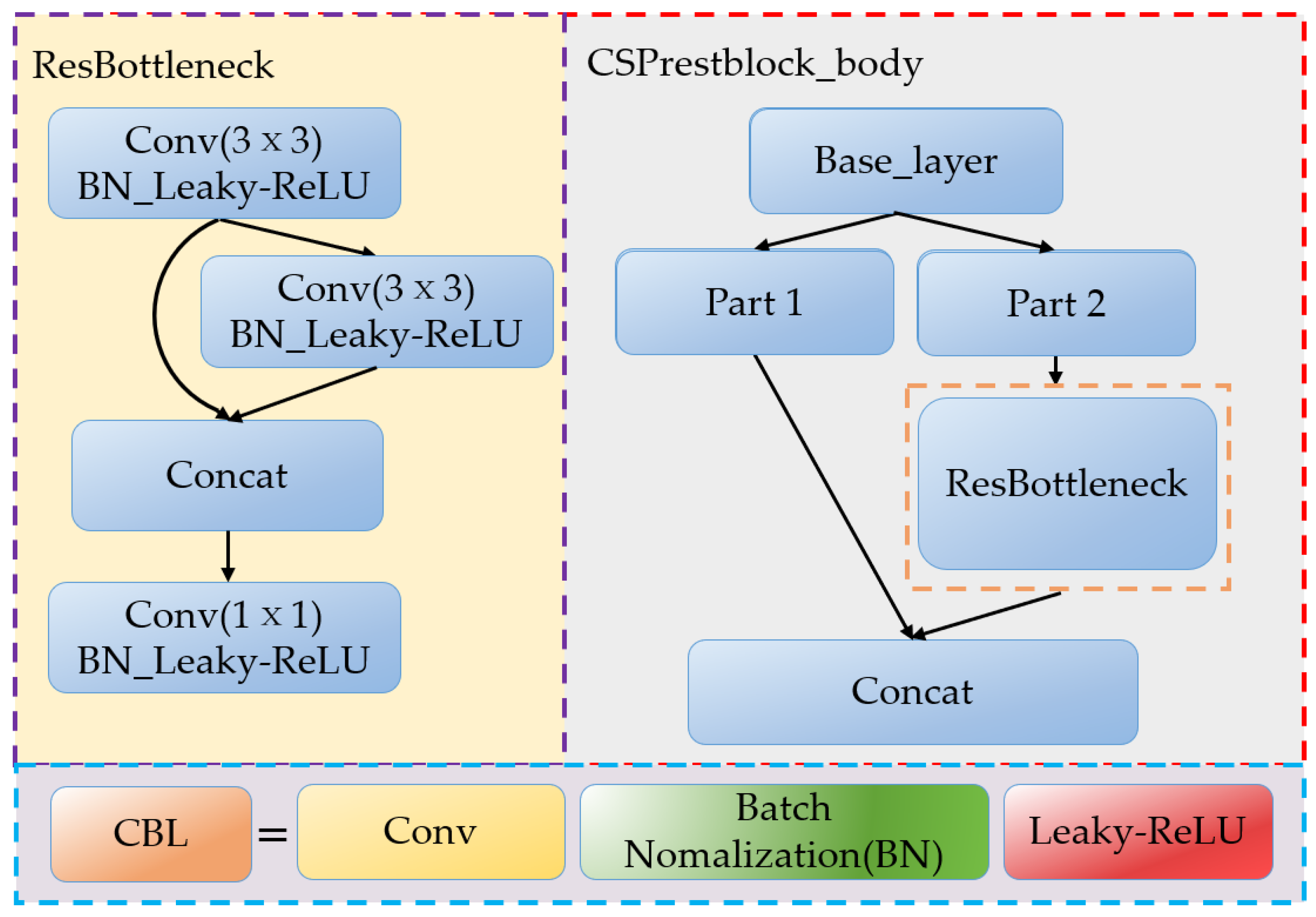
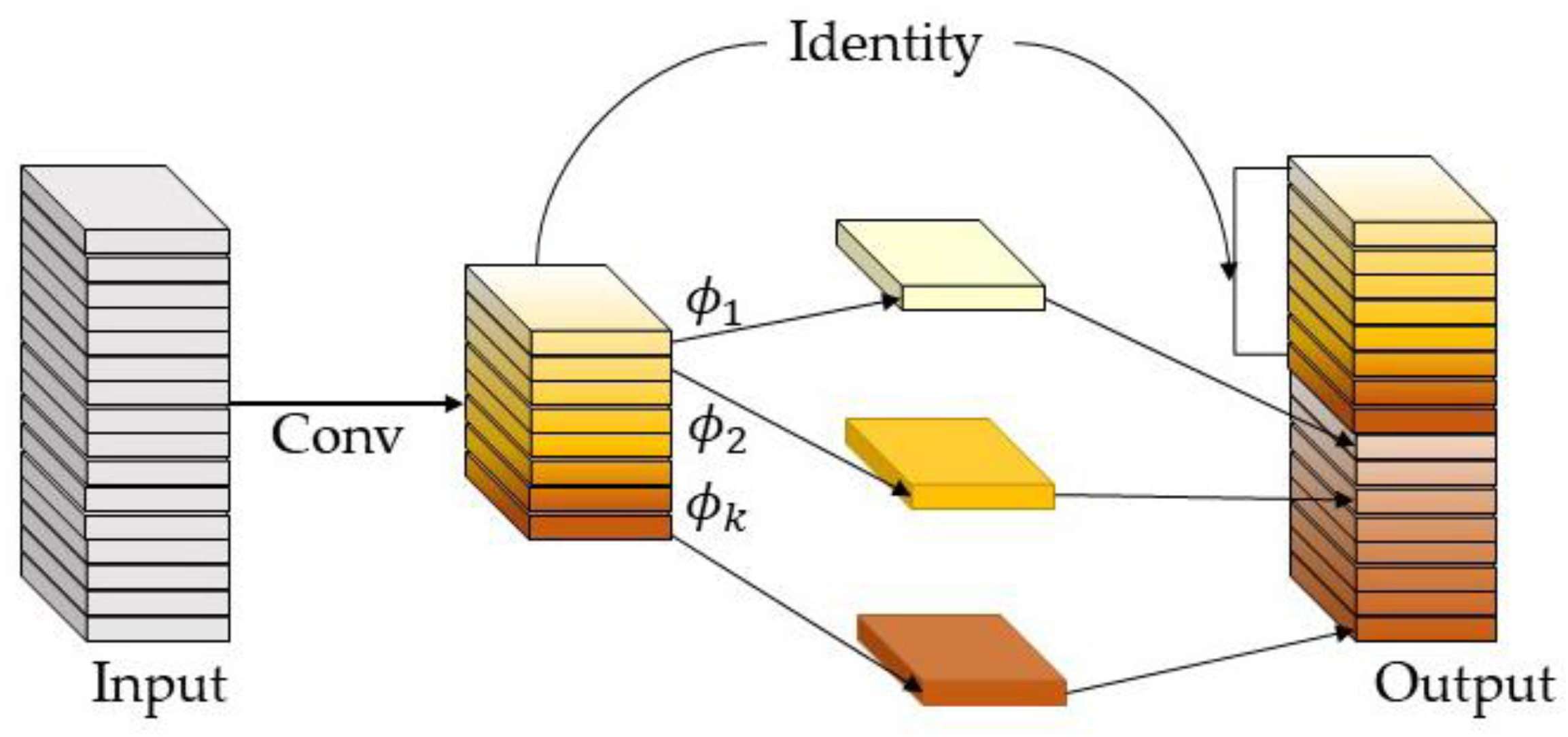
3.1.1. Improvement of Backbone Network

As shown in Section 2.1, the detection speed of the YOLOV4-Tiny method has substantially improved when compared with the YOLOV4 algorithm, but it still cannot realize the real-time operation of embedded underwater devices in a constrained environment.

In order to maintain the feature extraction capability of the backbone part, the proposed YOLOV4-Tinier algorithm still uses the CBL in the original network for the first two feature extraction layers. The backbone network of the YOLOV4-Tiny architecture contains three CSPresblock_body modules, which have multiple convolutional layers. Although the convolution operation can extract the features in the image, the convolution kernel contains a large number of parameters. Therefore, the original CSPresblock_body is replaced by Ghostblock_body, which is composed of a Ghost module, and the complex convolutional operation is replaced by a linear transformation, which effectively reduces the number of network parameters and the model size. The structure of Ghost module and Ghostblock_body is shown in Figure 2. The implementation process of the Ghost module [30] is divided into three steps: (1) Creating an intermediate feature map with fewer channels using 3 × 3 convolution. (2) Applying a series of linear adjustments to the feature maps to build more Ghost feature maps. (3) In the channel dimension, concatenating the feature maps which are created in the prior two phases. The implementation process of Ghostnet is shown in Figure 3 where ɸ represents the cheap transformations.

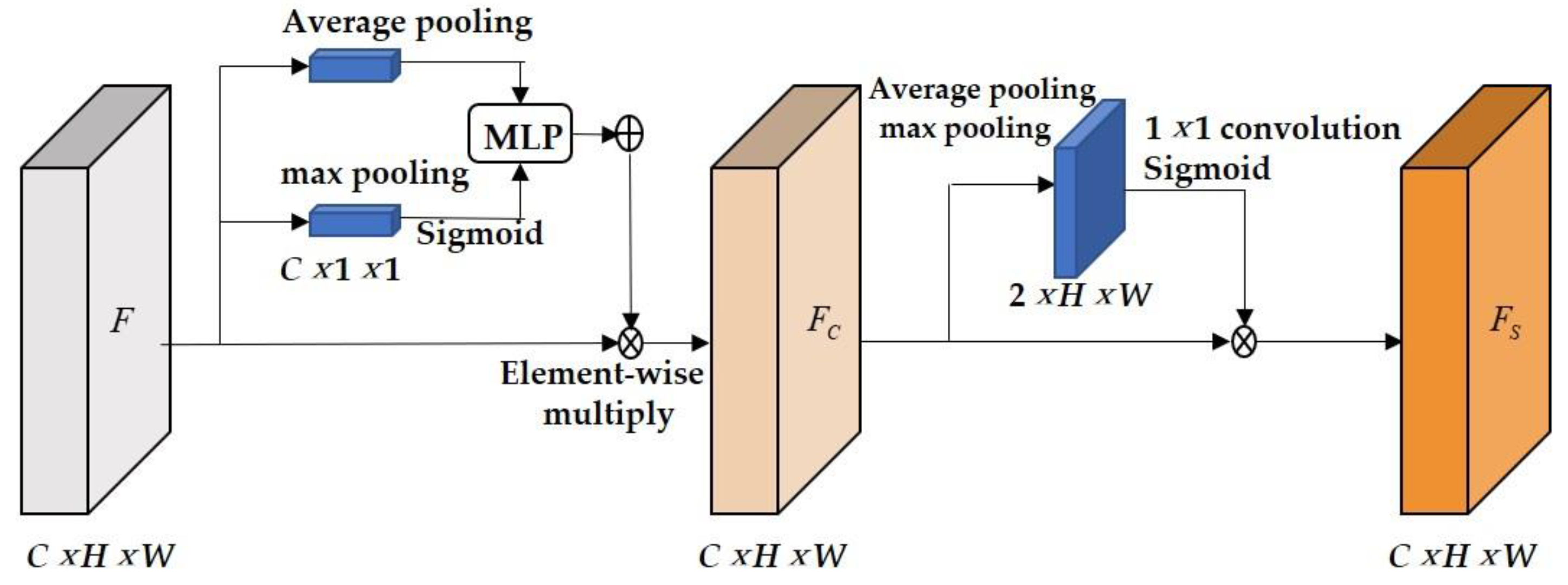
3.1.2. Improvement of the Neck Network

Using the Ghost module can increase the algorithm’s computation speed. However, the installation of the Ghost module will have an impact on the extraction of target data from the deep feature map. Additionally, the shallow feature map has a small receptive field that is suitable for the detection of small targets. However, the low-dimensional feature maps introduce a large amount of background noise, which impairs the accuracy of layered target detection. To address the aforementioned issues, this paper employs the convolutional block attention module (CBAM) proposed by Wu et al. [31]. It combines the convolution blocks of Channel and Spatial attention to process and transmit the effective features while suppressing the invalid features in order to improve target detection accuracy by tweaking a few parameters. Figure 4 depicts its structure. The channel attention module aggregates the spatial information of each channel through max pooling and average pooling, and obtains two 1 × 1 × C channel weight matrices, which are input into a Multilayer Perceptron (MLP) with shared parameters. Then, the element-wise summation is performed, and the addition result activated through Sigmoid to obtain the channel weight feature vector F_C; finally, element-wise multiplication is performed with the original feature map. For spatial attention, the feature map F_C output by the channel attention module is transmitted to the spatial attention module, and prossed by the average pooling and maximum pooling. Then, after splicing the feature graphs along the channel direction, a 1 × 1 convolution layer is input and activated by Sigmoid to conduct weight learning and multiply element by element with F_C. Finally, the spatial weight feature vector F_S is obtained, where C is the number of channels in the feature map and $H\times W$ is the size of the feature map.

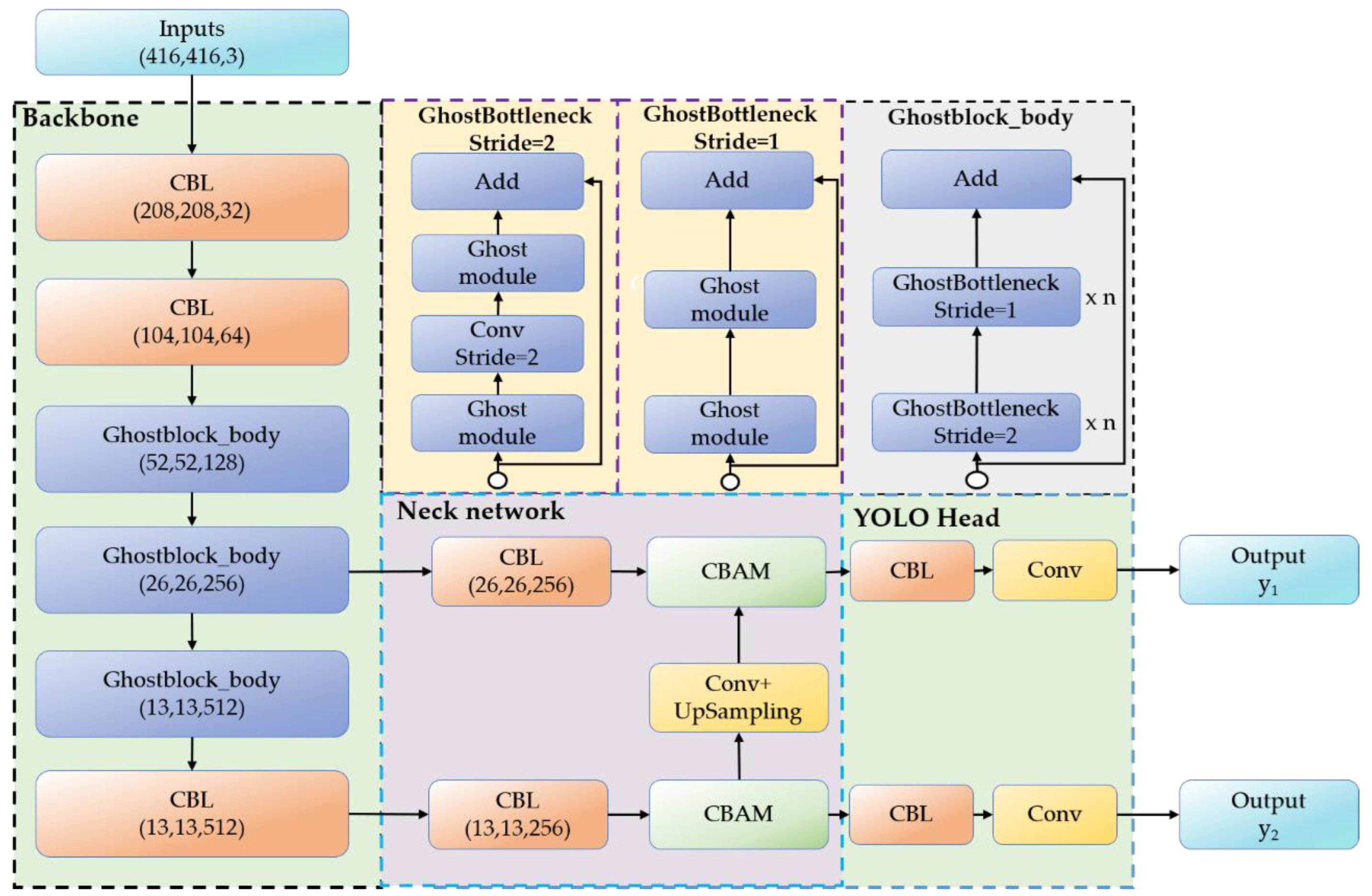
3.1.3. YOLOV4-Tinier Network Structure

Figure 2 shows the structure of the proposed YOLOV4-Tinier detection algorithm model. Firstly, the 416 × 416 pixel image is selected as the model input. In order to further reduce the calculations, we replace the 3 × 3 convolution with Ghost Module and stack it as Ghost Bottleneck on the basis of the CSPDarknet53-Tiny network to process feature layers of different dimensions. The shallow feature information is aggregated through two layers of CBL modules, and the feature dimension is changed to 104 × 104 × 64. Then, the features are further extracted through the four-layer Ghostblock_body, and two effective feature layers y₁ and y₂ are obtained. Among them, y₁ focuses on small and medium scale features, and y₂ focuses on large scale feature detection, with the dimensions 26 × 26 × 256 and 13 × 13 × 512. Then, the features extract more effective information through the two-layer CBL module and CBAM attention module. Finally, the processed feature information layer is used as the output to construct the Feature Pyramid Networks (FPN) structure. It combines the attention mechanism weights and performs feature fusion with the multi-scale feature level weights in order to realize feature fusion and reuse.

3.2. Improvement of the Input to the Proposed Underwater Data Augmentation Algorithm

In order to overcome the low quality of underwater images and the difficulty of uniform collection of different underwater objects, we propose an underwater data augmentation algorithm. Firstly, the Instance-Balance Augmentation algorithm is used to improve the distribution of datasets by copying images and adding disturbance. Then, the image restoration algorithm is used to improve the quality of underwater images. Finally, the Mosaic algorithm is introduced to enrich the image background information by splicing multiple images.

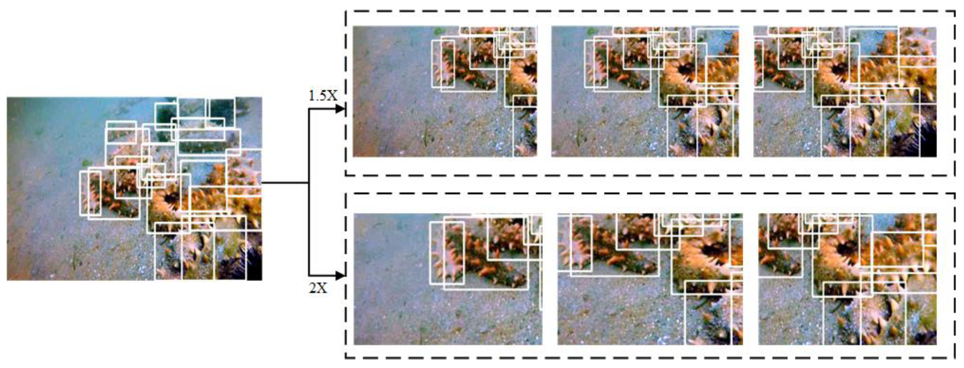
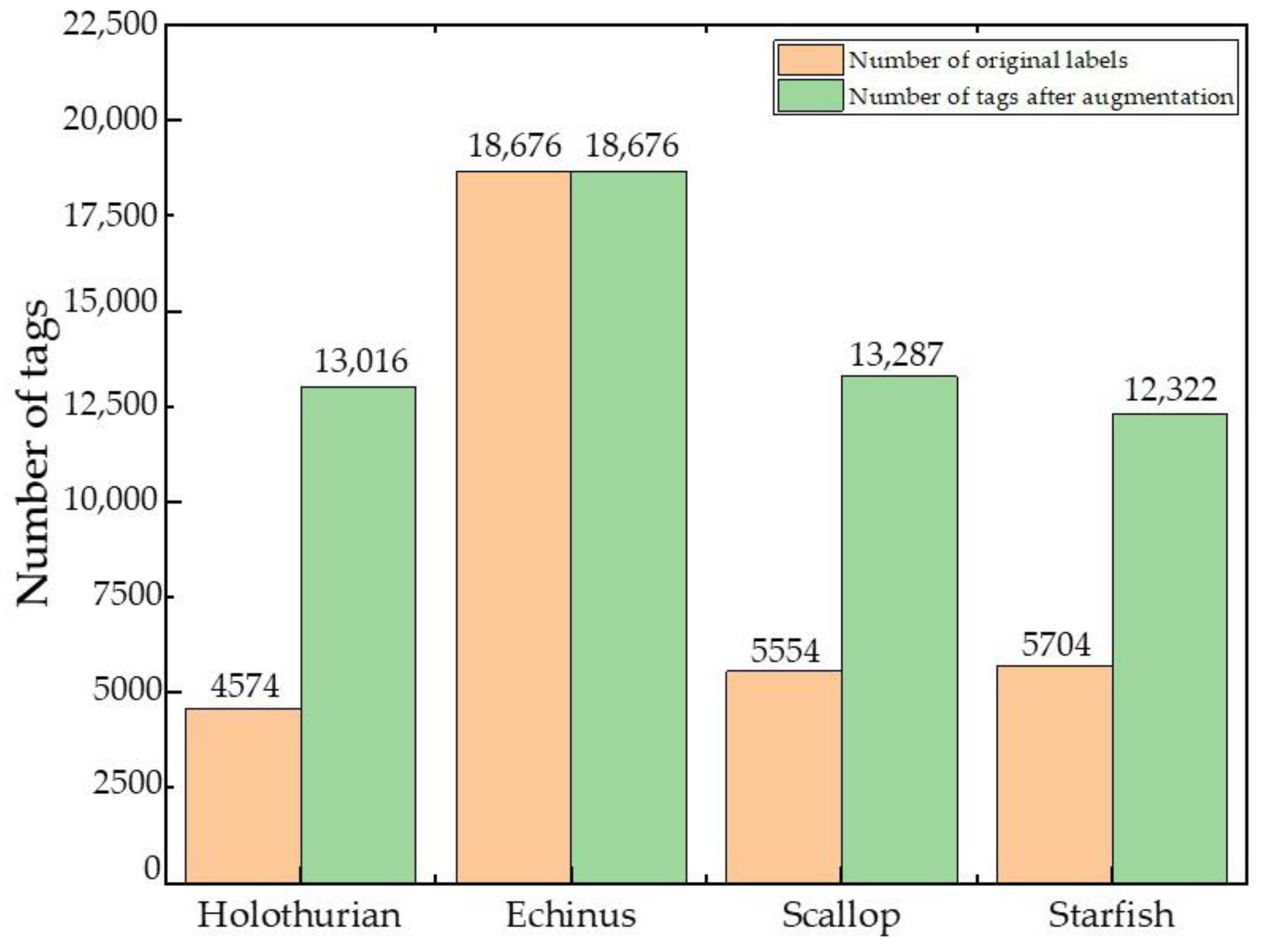
3.2.1. The Data Balance of the Proposed Underwater Data Augmentation Algorithm

Deep learning needs a large amount of data. Generally speaking, the more balanced the number of samples is, the better the prediction effect and generalization ability of the model are. However, the number of images in the dataset cannot meet the requirements or a large amount of data is distributed in some categories. To solve the above problems, the Instance-Balanced Augmentation algorithm [32] is introduced, which can not only increase the number of samples but also effectively improve the sample distribution.

Firstly, we enlarge the original image by 1.5 and 2 times, and then use the original size of the original image as the size of the sliding window. Movement is taken horizontally and vertically for three times on average in the form of a sliding window. The last image will obtain nine enhanced images equivalent to shift and scale. The algorithm steps are shown in Figure 5. In these sliding windows, select the optimal data containing desired targets to join the training set. There are certain rules in the process of selecting sliding windows. For example, the sliding window target with boundary overlap between the sliding window and the existing target at a certain step size will not be used, and the selection of the sliding window target will also refer to the distribution of the existing sample categories in the dataset. In order to enhance the original dataset, when the algorithm selects certain sliding window targets, it will change according to the resolution and scale and add some random disturbances. The white boxes in the image are the anchor boxes of the underwater targets which are pre-marked.

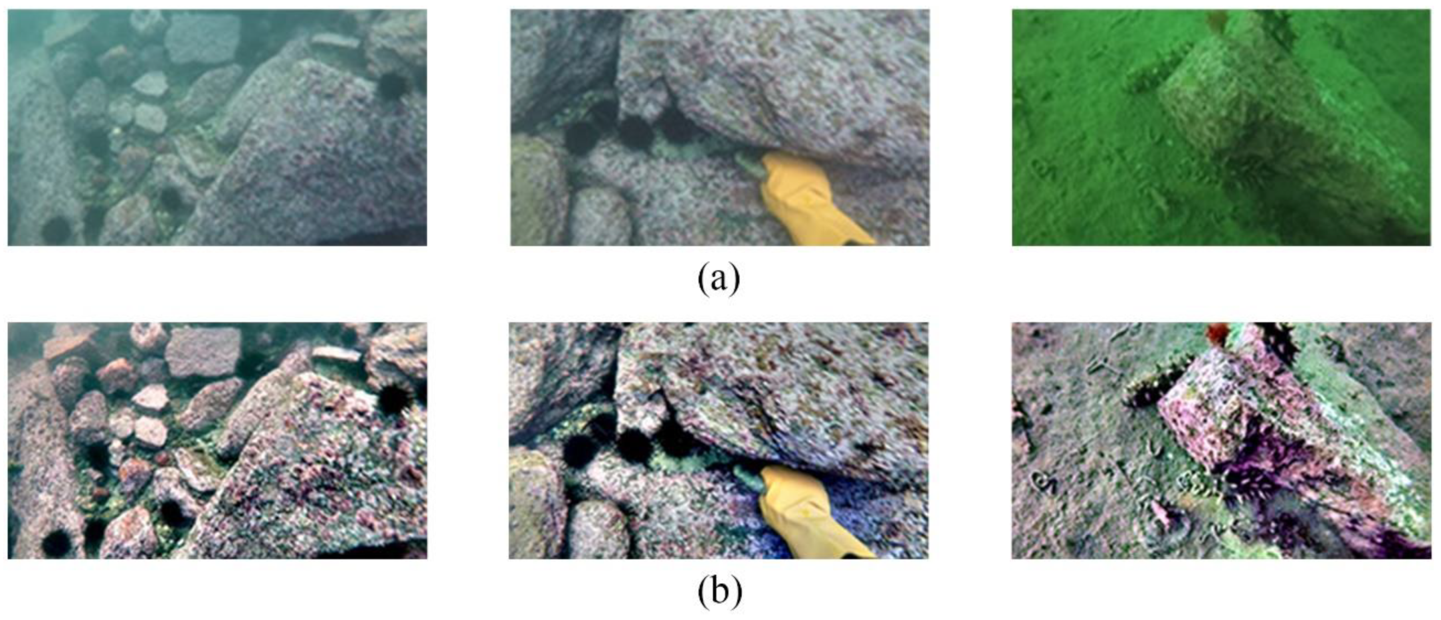
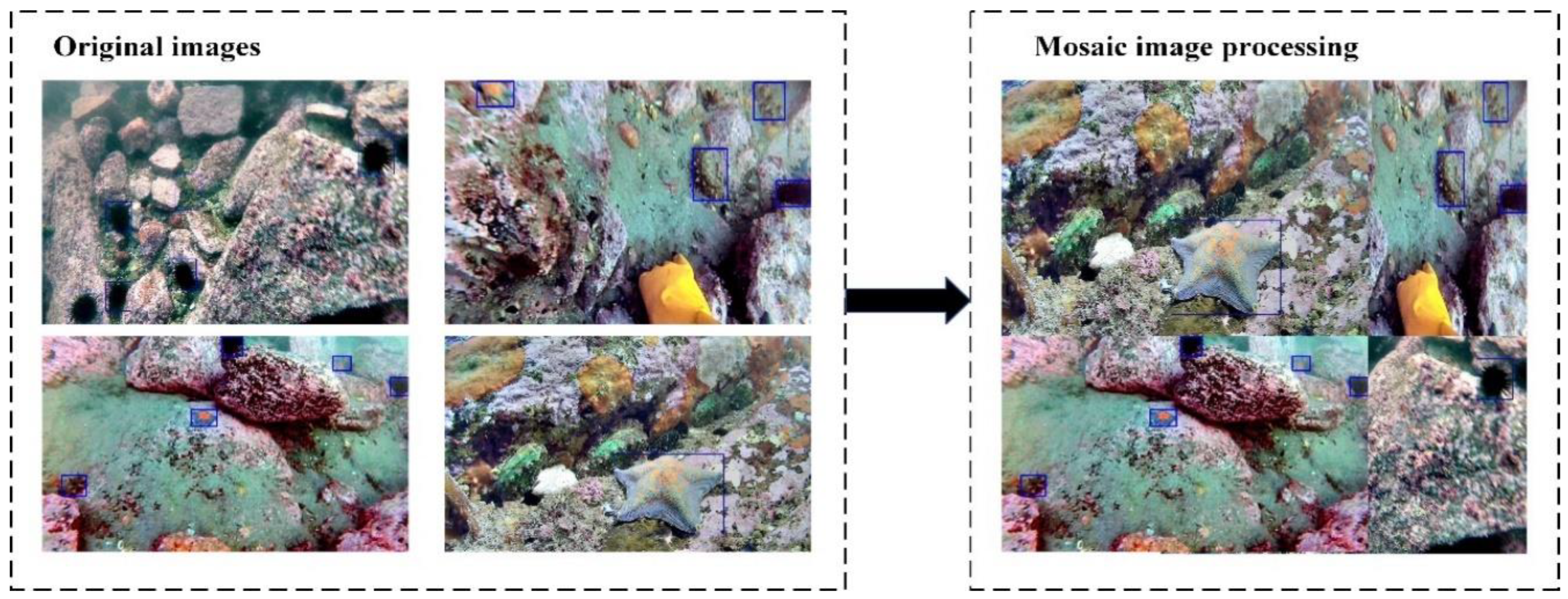
3.2.2. Image Restoration and Splice of Proposed Underwater Data Augmentation Algorithm

First, using the data balance algorithm introduced in Section 3.2.1 can expand the original dataset and improve data distribution. However, complex background and target details cannot be obtained only through simple image reproduction. At the same time, the dissolved organic compounds, inorganic substances, bubbles, and particles in the underwater environment lead to low contrast, chromatic aberration, and distortion of underwater images [33]. Therefore, in order to solve the above problems, we selected the BDYO algorithm (Based on Dark Channel Prior and Yin-Yang pair optimization) proposed by Yu Kun et al. [34] to repair underwater images. It can be seen in Figure 6 that the BDYO algorithm has a significant improvement in color and clarity compared to the original image. The balanced dataset is then processed by the Mosaic data augmentation algorithm. Four images are spliced into a new one and passed into the proposed network for learning so that the network can learn the information of four images at the same time. The results are shown in Figure 7. This method greatly enriches the background information of the object and effectively repairs the underwater images. The blue boxes in Figure 7 are the anchor boxes of the underwater targets which are pre-marked.

4. Experimental Settings

4.1. Experimental Environment

The experimental environment includes IntelXeonE3-1220V6 @3.00 GHz quad-core processor, 32GB RAM, and Nvidia GTX2080 Ti. All experiments were performed using CUDA 10.2 on PyTorch 1.5.1, Python 3.7, and Windows 10 platforms. The algorithm is written in the Windows 10 platform using the PyTorch framework.

4.2. Experimental Datasets

(a) Original image dataset: The underwater image labeling dataset provided by the official website of UPRC 2021. This dataset provides underwater target images of holothurian, echinus, scallop, and starfish, as well as their position coordinates in the images. There is a total of 5543 underwater optical images in .jpg format, with 4743 images in the training dataset and 800 images in the test dataset.

(b) Underwater data augmentation processing dataset: To balance the dataset, the original image is magnified by 1.5 times, and target extraction is performed using a sliding window of the same size as the original image. However, the dataset has an excessive amount of echinus, and there are numerous images with only one scallop, which easily leads to overfitting of the training model. Therefore, the sliding window must be limited: no enhancing processing is conducted if the sliding window comprises sea urchins or only one scallop image. The improved dataset has the following number of targets: 13,016 holothurians, 18,676 echinus, 13,287 scallops, and 12,322 starfish. As shown in Figure 8, the processed image category is balanced against the original dataset. Then, the balanced images are processed by underwater image restoration and Mosaic algorithm to produce a dataset with 18,982 pictures, including 14,236 training dataset and 4746 test dataset.

4.3. Parameter Settings

4.3.1. Training Parameter Settings

The input image size is uniformly 416 × 416 after processing, the initial learning rate is set to 0.0001, the momentum is 0.9, the weight decay is 0.0005, and the batch size is 16. The model trained for a total of 100 epochs.

4.3.2. Transfer Learning Parameter Settings

To speed up training, transfer learning is used to train the model. The underwater targets are trained using the feature information learned by YOLOV4-Tinier in the VOC dataset, and the pre-training model is frozen for 50 periods before being unfrozen. Figure 9 depicts the training results.

It can be seen from Figure 9 that, compared with random initialization, the convergence rate of the model is faster and the loss value of the model is lower in the training process of transfer learning.

4.4. Evaluation Indexes of Model Performance

To measure the performance of the model, the evaluation index introduced in this paper is as follows. (1) Precision (pre): represents the proportion of positive samples in the predicted positive samples. (2) Recall (rec): The proportion of positive examples in the sample that is correctly predicted. (3) mean Average Precision (mAP): The average of various types of detection precision (AP) to reflect the global detection performance of the model. (4) Frames per second (fps): The calculation speed of the model; the larger the value, the faster the calculation speed. The calculation formula of each evaluation index is as follows:

$$pre=\frac{TP}{TP+FP}$$

(5)

$$rec=\frac{TP}{TP+FN}$$

(6)

$$F_1=\frac{2\times pre\times rec}{pre\times rec}=\frac{2TP}{2TP\times FP\times FN}$$

(7)

$$AP={\displaystyle {\int }_0^1(pre\cdot rec)drec}$$

(8)

$$mAP=\frac{1}{c}{\displaystyle \sum _{i=1}^{c}A{P}_i}$$

(9)

where TP is True positive, FP is false positive, FN is false negative, and TN is true negative.

4.5. Experimental Results and Analysis

In order to verify the effectiveness of the proposed algorithm, four groups of experiments are conducted and analyzed for different detection models by using the evaluation indexes in Section 4.4. The experimental settings are as follows.

4.5.1. Effectiveness of Proposed Underwater Data Augmentation Algorithm

Three different datasets are used to test the effectiveness of the proposed underwater data augmentation algorithm: the original dataset, the dataset processed by the Mosaic algorithm, and the dataset processed by the underwater data augmentation algorithm. The proposed YOLOV4-Tinier model is used to run these three datasets. The results are shown in

Table 1. Comparison of the different datasets.

Datasets	AP (%)				[email protected]
	Starfish	Echinus	Holothurian	Scallop	(%)
Original dataset	49	39	29	4	30.05
Mosaic dataset	51	44	28	3	31.56
Proposed dataset	86	86	76	75	80.77

.

It can be found from Table 1 that, when using the YOLOV4-Tinier algorithm, compared with the original dataset and the Mosaic processing dataset, the proposed dataset greatly improves the detection precision of the trained model. Moreover, the detection accuracy of different types of targets is similar, indicating that the underwater data augmentation algorithm approach described in this research successfully improves the target feature extraction ability, balances the data distribution, and prevents overfitting.

4.5.2. Ablation Experiments for YOLOV4-Tinier

We used YOLOV4-Tiny as the foundation to check the model performance by utilizing various modules to test the efficacy of our proposed improved method.

Table 2. Ablation experiments from YOLOV4-Tiny to YOLOV4-Tinier on the proposed dataset.

YOLOV4-Tiny	GhostNet	CBAM	mAP (%)	Model Size (MB)
√			82.09	23.10
√	√		77.32	16.13
√		√	83.16	23.76
√	√	√	80.77	16.40

gives the results of mAP, fps, and model size of the ablation experiment.

The experimental results show that compared with YOLOV4-Tiny, the introduction of the Ghost module dramatically decreases the model size and fps when compared to YOLOV4-Tiny, while maintaining a high level of detection accuracy. The model size is decreased from 23.10 MB of YOLOV4-Tiny to 16.13 MB. On the basis of introducing Ghost modules, the employment of the CBAM attention module increases the mAP by 3.45% without adding too many parameters.

4.5.3. Real-Time Performance of YOLOV4-Tinier

The average test time and fps are selected as the measurement indexes of the real-time performance of the algorithm. We selected 3000 underwater images processed by the rich background data augmentation algorithm proposed in this paper to calculate the average detection time.

Table 3. Comparison of the real-time performance.

Model	Average Test Time (ms)	fps	Model Size (MB)
YOLOV3-Tiny	17.32	57.63	34.9
YOLOV4-Tiny	13.22	75.28	23.10
YOLOV4-Tinier	11.5	86.96	16.40

shows that the YOLOV4-Tinier algorithm has an average detection time of 11.5 ms and a frame rate of 86.96 fps. YOLOV3-Tiny and YOLOV4-Tiny, when compared to YOLOV4-Tinier, gain 17.32 ms and 57.63 fps and 13.22 ms and 75.28 fps, respectively. The YOLOV4-Tinier detection model is only 71% of the size of YOLOV4-Tiny and 47% of the size of YOLOV3-Tiny. The YOLOV4-Tinier algorithm, as can be observed, has reduced complexity, a faster calculation speed, and a smaller model size, making it more ideal for underwater real-time detection.

4.5.4. Performance of mAP on the Proposed Dataset

Due to the fact that Faster-RCNN, YOLOV3-Tiny, YOLOV4-Tiny, and our proposed techniques are lightweight deep learning algorithms, but YOLOV3 and YOLOV4 methods are not, we only compare our proposed method to lightweight algorithms in the following analysis. The model is trained on a dataset processed by the underwater data augmentation algorithm, and the uniform image size (416 × 416) is utilized as the input to keep the parameters under strict control. The experimental results are shown in

Table 4. Comparison of the detection accuracy of different models.

Model	Scallop		Echinus		Holothurian		Starfish		mAP
	Precision	Recall	Precision	Recall	Precision	Recall	Precision	Recall	@0.5
Faster-RCNN	49.09	84.97	50.11	79.59	40.64	74.17	61.14	86.29	74.91
YOLOV3-	88.35	55.3	88.93	34.21	90.79	55	90.05	60.17	67.72
Tiny
YOLOV4-Tiny	87.7	73.86	91.21	53.83	89.2	57.58	91.56	74.39	82.09
YOLOV4	87.05	72.14	92.46	48.98	88.98	56.89	90.84	73.44	80.77
-Tinier

.

It can be seen from Table 4 that the detection performance of the Faster-RCNN is good, since it creates a prior frame in advance and adds a feature fusion module. However, because no image pyramid has been built, it is unable to efficiently utilize information from the shallow layer, making it insensitive to small-scale targets. Furthermore, the proposed technique is substantially larger than the one-stage detection model. YOLOV4-Tinier uses a more complex network and multiple training procedures compared to the YOLOV3-Tiny algorithm, and its detection precision is enhanced by 13.05%. The proposed algorithm’s average accuracy is 1.32% lower than that of YOLOV4-Tiny; however, the model’s size is just half that of YOLOV4-Tiny. At the same time, as shown in Table 4, the addition of the CBAM module successfully reduces the influence of background noise on detection, resulting in improved YOLOV4-Tinier accuracy and recall, as well as a lower number of holothurian and echinus misdetections. As a result, YOLOV4-Tinier performs well in the above algorithms.

The detection results were visualized on the URPC underwater datasets and proposed dataset in Figure 10 and Figure 11. It was observed that the identification results of the proposed algorithm in the study were more accurate, with less misrecognition or missed recognition, while the Faster-RCNN algorithm and YOLOV3-Tiny algorithm have many false and missing detection cases in target detection. Additionally, the detection performance of the proposed dataset is significantly better than the URPC underwater datasets. In addition, we can see from Table 3 that our detection speed and model size are far less than those of the other two classical fast detection algorithms, which makes our detection algorithm more relevant in the application of small underwater equipment with limited computing power.

5. Conclusions

This paper proposes the YOLOV4-Tinier detection algorithm and the underwater data augmentation algorithm. The proposed model uses the Ghost module and adds the CBAM attention module to increase detection speed while maintaining high accuracy. Then, the underwater data augmentation algorithm is proposed to improve the image quality and make the distribution of data reasonable. Experiments show that the proposed algorithm has good detection accuracy. The average detection precision of the YOLOV4-Tinier algorithm reaches 80.77%, which is similar to YOLOV4-Tiny. The model size is reduced by 29% and the detection speed is increased by 15.51%. The YOLOV4-Tinier algorithm can further improve the speed of model calculation and is more suitable for embedded device development, while the underwater data augmentation algorithm provides an idea for obtaining high-quality underwater image datasets.

References

1. Chen, Y.; Ling, Y.; Zhang, L. Accurate Fish Detection under Marine Background Noise Based on the Retinex Enhancement Algorithm and CNN. J. Mar. Sci. Eng. 2022, 10, 878. [Google Scholar] [CrossRef]
2. Zhang, M.; Xu, S.; Song, W.; He, Q.; Wei, Q. Lightweight Underwater Object Detection Based on YOLO v4 and Multi-Scale Attentional Feature Fusion. Remote Sens. 2021, 13, 4706. [Google Scholar]
3. Sung, M.; Yu, S.; Girdhar, Y. Vision based real-time fish detection using convolutional neural network. In Proceedings of the OCEANS 2017, Aberdeen, DC, USA, 19–22 June 2017. [Google Scholar]
4. Kou, L.; Xiang, J.; Bian, J. Controllability Analysis of a Quadrotor-like Autonomous Underwater Vehicle. In Proceedings of the 2018 IEEE 27th International Symposium on Industrial Electronics (ISIE), Cairns, Qld, Australia, 13–15 June 2018. [Google Scholar]
5. Drews, J.P.; Nascimento, D.; Moraes, F. Transmission Estimation in Underwater Single Images. In Proceedings of the 2013 IEEE International Conference on Computer Vision Workshops, Sydney, NSW, Australia, 2–8 December 2013. [Google Scholar]
6. Palazzo, Simone, Francesca Fish species identification in real-life underwater images. In Proceedings of the 3rd ACM International Workshop on Multimedia Analysis for Ecological Data, Lisboa, Portugal, 10–14 October 2022.
7. Qin, H.; Li, J.; Peng, Y.; Zhang, C. DeepFish: Accurate underwater live fish recognition with a deep architecture. Neurocomputing 2016, 187, 49–58. [Google Scholar] [CrossRef]
8. Han, F.; Yao, J.; Zhu, H.; Wang, C. Marine organism detection and classification from underwater vision based on the deep CNN method. Math. Probl. Eng. 2020, 2020, 3937580. [Google Scholar] [CrossRef]
9. Arvind, C.S.; Prajwal, R.; Bhat, P.N. Fish detection and tracking in pisciculture environment using deep instance segmentation. In Proceedings of the TENCON IEEE Region 10 Conference, Osaka, Japan, 16–19 November 2020. [Google Scholar]
10. He, K.; Gkioxari, G.; Dollar, P.; Girshick, R. Mask r-cnn. In Proceedings of the IEEE International Conference on Computer Vision, Seoul, Republic of Korea, 20–23 June 1995. [Google Scholar]
11. Held, D.; Thrun, S.; Savarese, S. Learning to track at 100 fps with deep regression networks. In Proceedings of the European Conference on Computer Vision, Glasgow, UK, 23–28 August 2020. [Google Scholar]
12. Li, J.; Xu, C.; Jiang, L.; Xiao, Y.; Deng, L. Detection and analysis of behavior trajectory for sea cucumbers based on deep learning. IEEE Access 2019, 99, 18832–18840. [Google Scholar] [CrossRef]
13. Liu, W.; Anguelov, D.; Erhan, D.; Szegedy, C. SSD: Single shot multibox detector. In Proceedings of the European Conference on Computer Vision, Amsterdam, The Netherlands, 8–16 October 2016. [Google Scholar]
14. Wu, H.; He, S.; Deng, Z.; Kou, L.; Huang, K.; Sou, F.; Cao, Z. Fishery monitoring system with AUV based on YOLO and SGBM. In Proceedings of the 2019 Chinese Control Conference (CCC), Guangzhou, China, 3–5 June 2019. [Google Scholar]
15. Hu, X.; Liu, Y.; Zhao, Z.; Liu, J.; Yang, X.; Sun, C.; Zhou, C. Real-time detection of uneaten feed pellets in underwater images for aquaculture using an improved YOLO-V4 network. Comput. Electron. Agric. 2021, 185, 106–135. [Google Scholar] [CrossRef]
16. Zhao, T.T.; Xiao, L.Y.; Zhi, Y.Z.; Tao, F. MobileNet-Yolo based wildlife detection model: A case study in Yunnan Tongbiguan Nature Reserve. China J. Intell. Fuzzy. Syst. 2021, 41, 2171–2181. [Google Scholar] [CrossRef]
17. Fang, W.; Wang, L.; Ren, P. Tinier-YOLO: A real-time object detection method for constrained environments. IEEE Access 2019, 99, 1935–1944. [Google Scholar] [CrossRef]
18. Jiang, Z.C.; Zhao, L.; Li, S.; Jia, Y. Real-time object detection method based on improver YOLOV4-Tiny. In Proceedings of the Conference on Computer Vision and Pattern Recognition, Seattle, WA, USA, 13–19 June 2020. [Google Scholar]
19. Hsiao, Y.H.; Cheng, C.C.; Lin, S.L. Real-world underwater fish recognition and identification using sparse representation. Ecol. Inform. 2014, 23, 13–21. [Google Scholar] [CrossRef]
20. Jiao, Q.; Liu, M.; Ning, B.; Zhao, F.; Dong, L.; Kong, L. Image Dehazing Based on Local and Non-Local Features. Fractal. Fract. 2022, 6, 262. [Google Scholar] [CrossRef]
21. Yun, S.; Han, D.; Oh, S.J.; Chun, S.; Choe, J.; Yoo, Y. CutMix: Regularization Strategy to Train Strong Classifiers with Localizable Features. In Proceedings of the CVF International Conference on Computer Vision, Seoul, Republic of Korea, 20–26 October 2019. [Google Scholar]
22. Bochkovskiy, A.; Wang, C.Y.; Liao, H.Y.M. Yolov4: Optimal speed and accuracy of object detection. arXiv 2020, arXiv:2004.10934. [Google Scholar]
23. NgoGia, T.; Li, Y.; Jin, D.; Guo, J.; Li, J.; Tang, Q. Real-Time Sea Cucumber Detection Based on YOLOv4-Tiny and Transfer Learning Using Data Augmentation. In Proceedings of the International Conference on Swarm Intelligence, Qingdao, China, 17–20 July 2021. [Google Scholar]
24. Cai, Y.; Luan, T.; Gao, H.; Wang, H.; Chen, L.; Li, Y.; Li, Z. YOLOv4-5D: An Effective and Efficient Object Detector for Autonomous Driving. IEEE Trans. Instrum. Meas. 2021, 70, 4503613. [Google Scholar]
25. Li, X.; Pan, J.; Xie, F.; Zeng, J.; Li, Q.; Huang, X. Fast and accurate green pepper detection in complex backgrounds via an improved Yolov4-tiny model. Comput. Electron. 2021, 191, 106–115. [Google Scholar] [CrossRef]
26. Wang, C.; Liao, H.; Wu, Y. CSPNet: A new backbone that can enhance learning capability of CNN. In Proceedings of the IEEE Conference on Computer Vision and Pattern Recognition, Seattle, WA, USA, 13–19 June 2020. [Google Scholar]
27. He, K.M.; Xiang, Y.Z.; Shao, Q.R.; Jian, S. Deep Residual Learning for Image Recognition. In Proceedings of the IEEE Conference on Computer Vision and Pattern Recognition, Boston, MA, USA, 7–12 June 2015. [Google Scholar]
28. Lin, T.; Dollár, P.; Girshick, R. Feature pyramid networks for object detection. In Proceedings of the IEEE Conference on Computer Vision and Pattern Recognition, Honolulu, HI, USA, 21–26 July 2017. [Google Scholar]
29. Zheng, Z.; Wang, P.; Liu, W. Distance-IoU loss: Faster and better learning for bounding box regression. In Proceedings of the IEEE Conference on Artificial Intelligence, New York, NY, USA, 7–12 February 2020. [Google Scholar]
30. Han, K.; Wang, Y.; Tian, Q.; Guo, J.; Xu, C. GhostNet: More Features from Cheap Operations. In Proceedings of the IEEE Conference on Computer Vision and Pattern Recognition, Seattle, WA, USA, 13–19 June 2020. [Google Scholar]
31. Woo, S.; Park, J.; Lee, J.Y.; Kweon, I.S. Cbam: Convolutional block attention module. In Proceedings of the European Conference on Computer Vision (ECCV), Munich, Germany, 8–14 September 2018. [Google Scholar]
32. Wang, H.; Wang, Q.; Yang, F.; Zhang, W.; Zuo, W. Data augmentation for object detection via progressive and selective instance-switching. arXiv 2019, arXiv:1906.00358. [Google Scholar]
33. Amer, K.O.; Elbouz, M.; Alfalou, A.; Brosseau, C. Enhancing underwater optical imaging by using a low-pass polarization filter. Opt. Express 2019, 27, 621–643. [Google Scholar] [CrossRef] [PubMed]
34. Yu, K.; Cheng, Y.F.; Li, L.; Zhang, K.H.; Liu, Y.F. Underwater Image Restoration via DCP and Yin–Yang Pair Optimization. J. Mar. Sci. Eng. 2022, 10, 360. [Google Scholar] [CrossRef]
Figure 1. The network structure of CBL and CSPrestblock_body.
Jmse 10 01821 g001
Figure 2. The network structure of YOLOV4-Tinier.
Jmse 10 01821 g002
Figure 3. The Ghost module.
Jmse 10 01821 g003
Figure 4. CBAM attention module implementation process.
Jmse 10 01821 g004
Figure 5. Instance-Balanced Augmentation algorithm.
Jmse 10 01821 g005
Figure 6. Comparison of (a) original images and (b) BDYO algorithm output images.
Jmse 10 01821 g006
Figure 7. Schematic diagram of the Mosaic algorithm.
Jmse 10 01821 g007
Figure 8. Number of targets after Instance-Balance Augmentation.
Jmse 10 01821 g008
Figure 9. Loss function graph for different training methods. (a) The random initialization. (b) transfer learning.
Jmse 10 01821 g009
Figure 10. Detection results of different detection algorithms on the URPC dataset. (a) Faster-RCNN test results, (b) YOLOV3-Tiny test results, and (c) YOLOV4-Tinier test results.
Jmse 10 01821 g010
Figure 11. Detection results of different detection algorithms on the proposed dataset. (a) Faster-RCNN test results, (b) YOLOV3-Tiny test results, and (c) YOLOV4-Tinier test results.
Jmse 10 01821 g011