
Overall Scheduling Model for Vessels Scheduling and Berth Allocation for Ports with Restricted Channels That Considers Carbon Emissions


Abstract
:1. Introduction
2. Related Literature
3. Problem Description
- The resources required for inbound and outbound operations: channels, tugs, and berths
- The requirement for a reasonable vessel service sequence
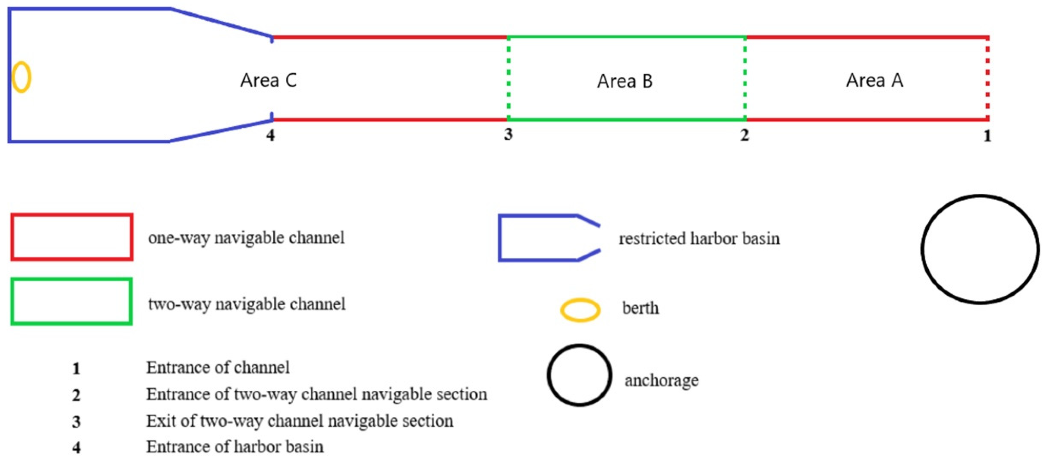
- The port’s navigation rules
- The safe time intervals needed to ensure the safety of navigation
- The tidal time windows for large vessels
- The physical factors and service types of the berth
- The distance between berths and the stockyard space in the yard
- The service times of different vessels using the same berth
- The carbon emissions of vessels (in relation to reasonable speed arrangements)
4. Mathematical Model and Formulas
4.1. Model Assumptions
- It is assumed that the time for all tugs to arrive at the inbound and outbound vessels is the same, and the distance from all berths to the entrance of the harbor basin is the same. This is based on the reasonable assumption that the distances within the harbor basin are small and have little impact on the overall scheduling.
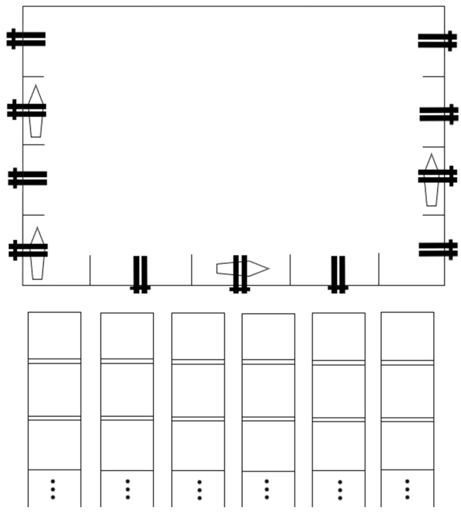
- In order to highlight the research focus, the yard and reclaimer allocation and scheduling are not considered at this stage. Therefore, it is assumed that there will be sufficient yard and reclaimer resources in the port to meet the needs of loading and unloading. As shown in Figure 2, the stockyard spaces in the yard are discrete. Each vessel is allocated stockyard spaces before entering the port to avoid any conflict.
- It is assumed that there are sufficient pilots at the pilot station and sufficient resources for wharf loading and unloading. The weather and visibility are assumed to be good and the pilot and captain to be experienced. It is also assumed that no accidents occur during navigation.
4.2. Mathematical Model
5. Algorithm Design
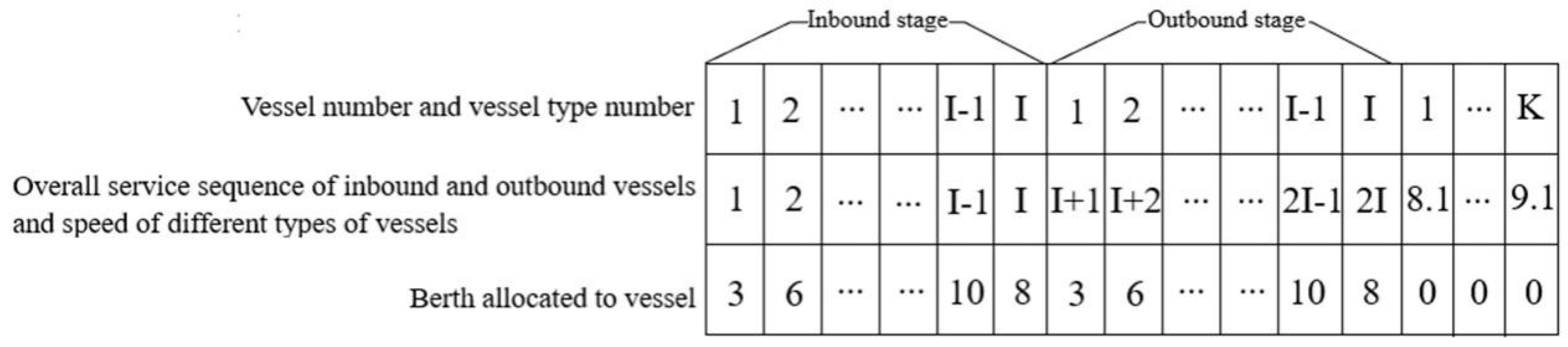
5.1. Gene Coding and Population Initialization
5.2. Fitness, Selection, Crossover, and Mutation
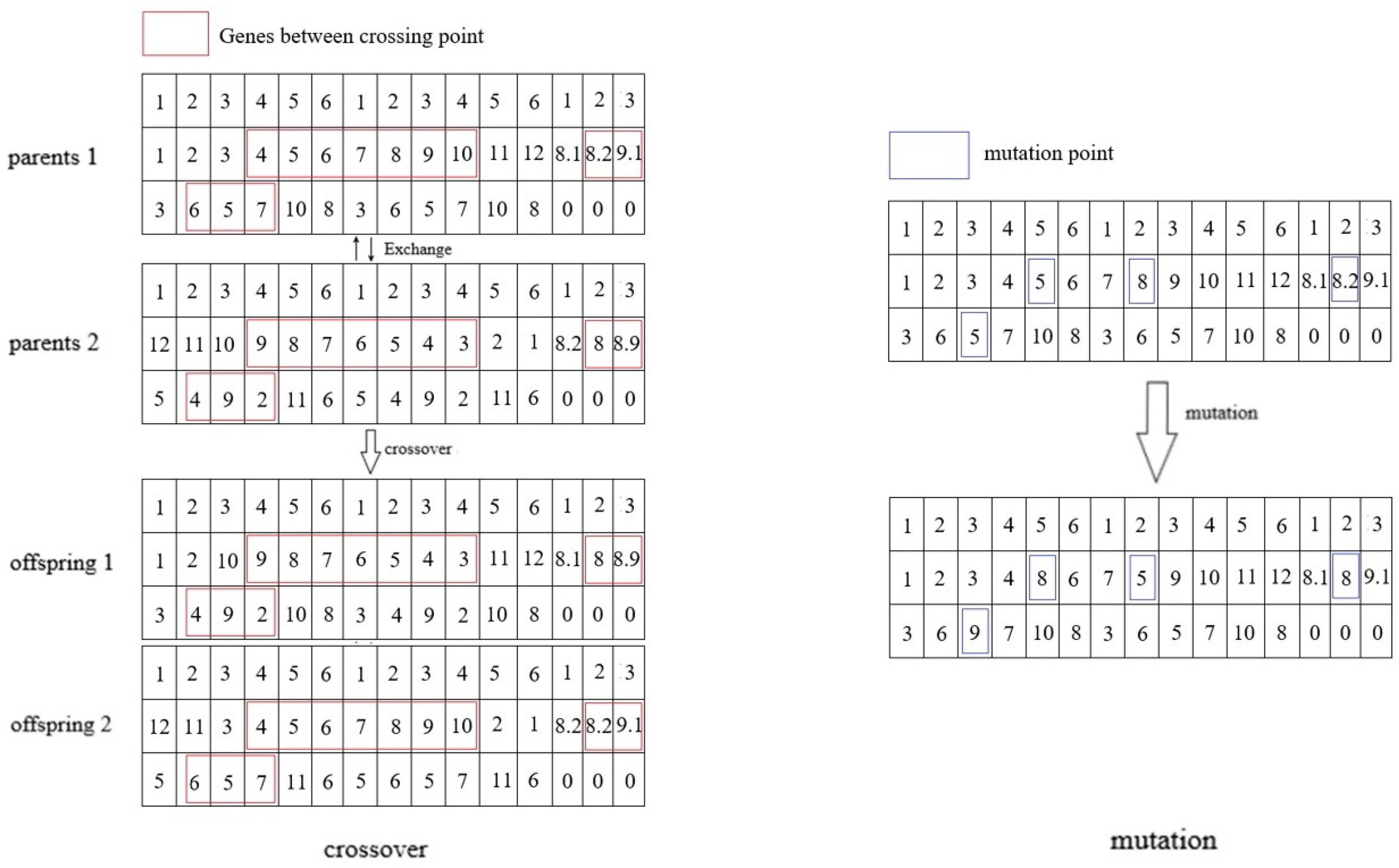
- After the crossover operation has been determined based on the crossover probability, two numbers between 0 and 2I are randomly generated as the crossover points, and the genes between the service sequence encoding crossover points of two parents are taken as the selected genes.
- Child 1 is generated with the same gene and location as the selected gene of parent 1.
- The position of the selected gene of parent 1 in parent 2 is found; the remaining genes of parent 2 are added to child 1 in order.
- Similarly, the selected gene of parent 2 is used to generate child 2.
- After the crossover operation has been determined by the crossover probability, two numbers between 0 and I are randomly generated, and the genes between the berth coding intersections of the two parents are selected as the selected genes.
- The selected genes of the berth codes of the two parents are exchanged.
- The 1-I genes of child 1 are copied to gene positions I + 1 to I + I; the same operation is then performed on child 2 to generate two new berth codes for the offspring.
- After the crossover operation has been determined by the crossover probability, two numbers between 0 and K are randomly generated as the intersection points, and the genes between the intersection points of the speed codes of the two parents are selected as the genes.
- The selected genes of the speed codes of the two parents are exchanged to generate two new speed codes for the offspring.
5.3. Elite Retention Policy
5.4. Adaptive Probability and Double-Population Strategy
| Algorithm 1: NSGA-II-DP |
| Algorithm parameters: chromosome (p), chromosome number (popsize), current algebra generation, upper limit on number of iterations (maxgeneration), maximum crossover probability (pcmax), minimum crossover probability (pcmin), maximum mutation probability (pmmax), minimum mutation probability (pmmin), best set of nondominated solutions of each generation (L1), objective function of Pareto solution (bestD), Pareto optimal solution set (bestpop) |
| 1: initial population [pop1, pop2] = {p1, p2, ppopsize−1, ppopsize} |
| 2: globalD←Inf |
| 3: generation←1 |
| 4: while (generation < maxgeneration) do |
| 5: if (generation = 1) then |
| 6: [pop1, pop2]←correction(pop1, pop2) |
| 7: [D1, D2]←calculate fitness(pop1, pop2) |
| 8: go to line 14 |
| 9: else |
| 10: [pop1, pop2]←[nnewpop1, nnewpop2] |
| 11: [D1, D2]←[newD1, newD2] |
| 12: go to line 14 |
| 13: end if |
| 14: [pops1, pops2]←selection(pop1, pop2) |
| 15: [popc1, popc2]←crossover(pops1, pops2, pcmax, pcmin) |
| 16: [popm1, popm2]←mutation(popc1, popc2, pmmax, pmmin) |
| 17: [popo1, popo2]←correction(popm1, popm2) |
| 18: [Do1, Do2]←calculate fitness(popo1, popo2) |
| 19: combinepop1←{pop1, popo1} |
| 20: combineD1←{D1, Do1} 21: combinepop2←{pop2, popo2} 22: combineD2←{D2, Do2} |
| 23: [newpop1, L11]←elite retention(combineD1, combinepop1) 24: [newpop2, L12]←elite retention(combineD2, combinepop2) 25: [nnewpop1, nnewpop2]←Dual Population(newpop1, L11, newpop2, L12) 26: [newD1, newD2]←calculate fitness(nnewpop1, nnewpop2) 27: combinepop←{nnewpop1, nnewpop2} 28: combineD ←{newD1, newD2} 29: L1←elite retention(combineD, combinepop) |
| 30: bestpop←L1 31: bestD←calculate fitness(L1) |
| 32: generation←generation + 1 |
| 33: end while |
| 34: output: bestpop, bestD |
6. Case Study
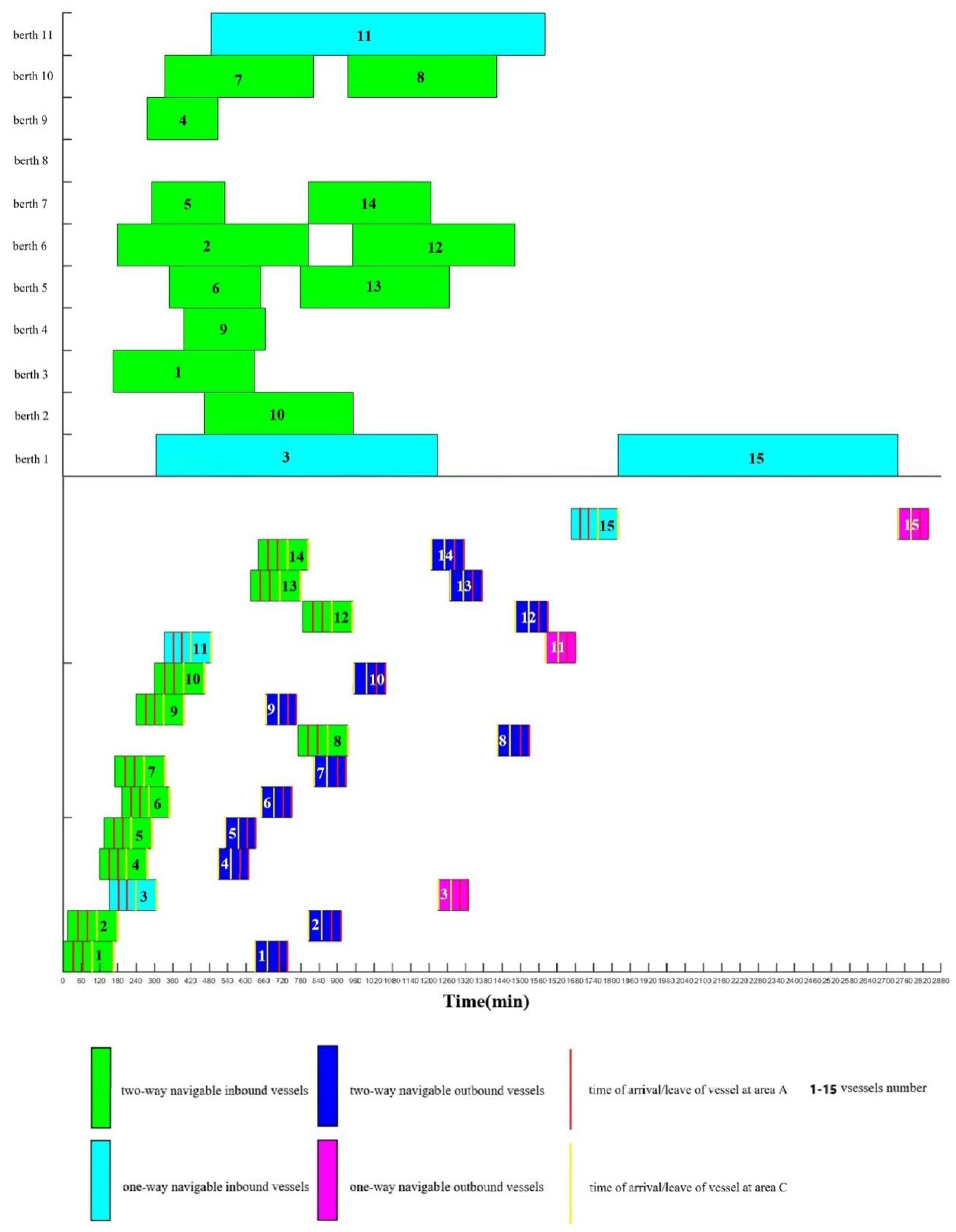
6.1. Case Study
6.2. Rationality Verification
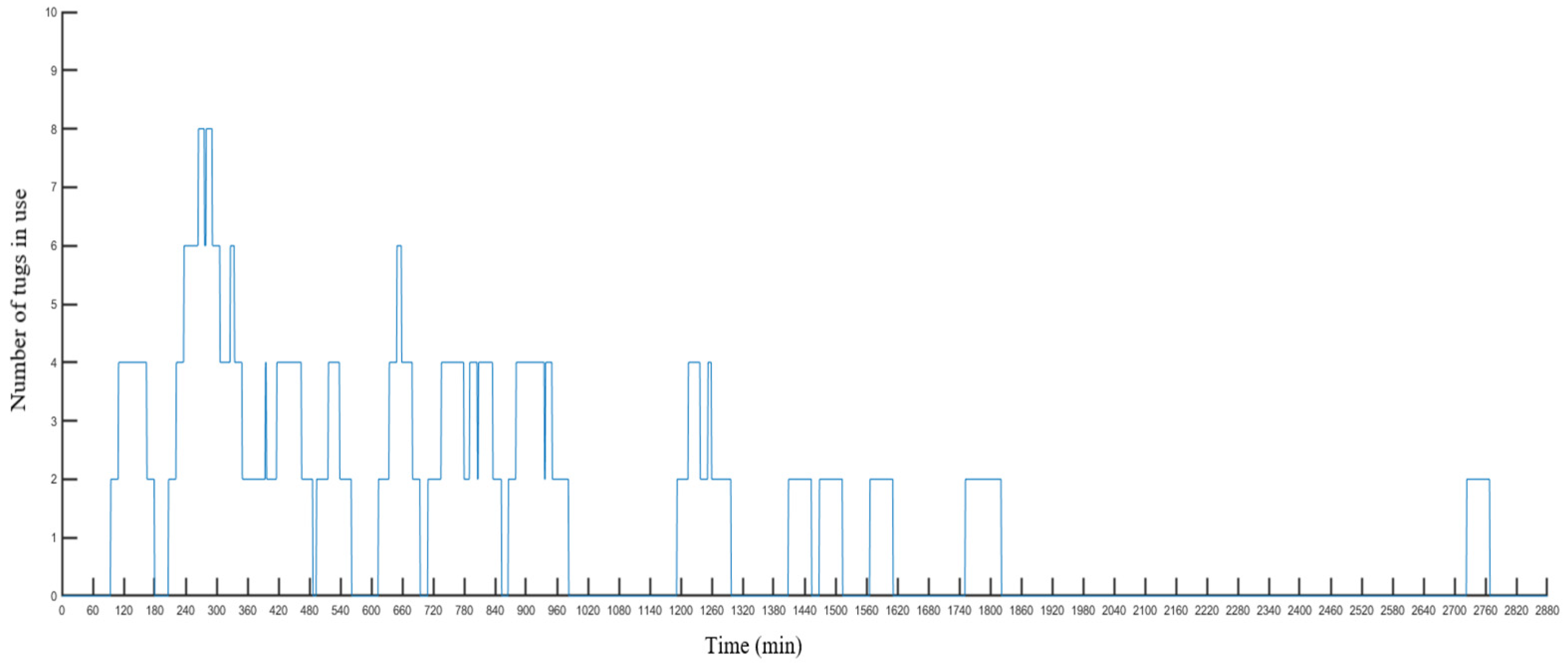
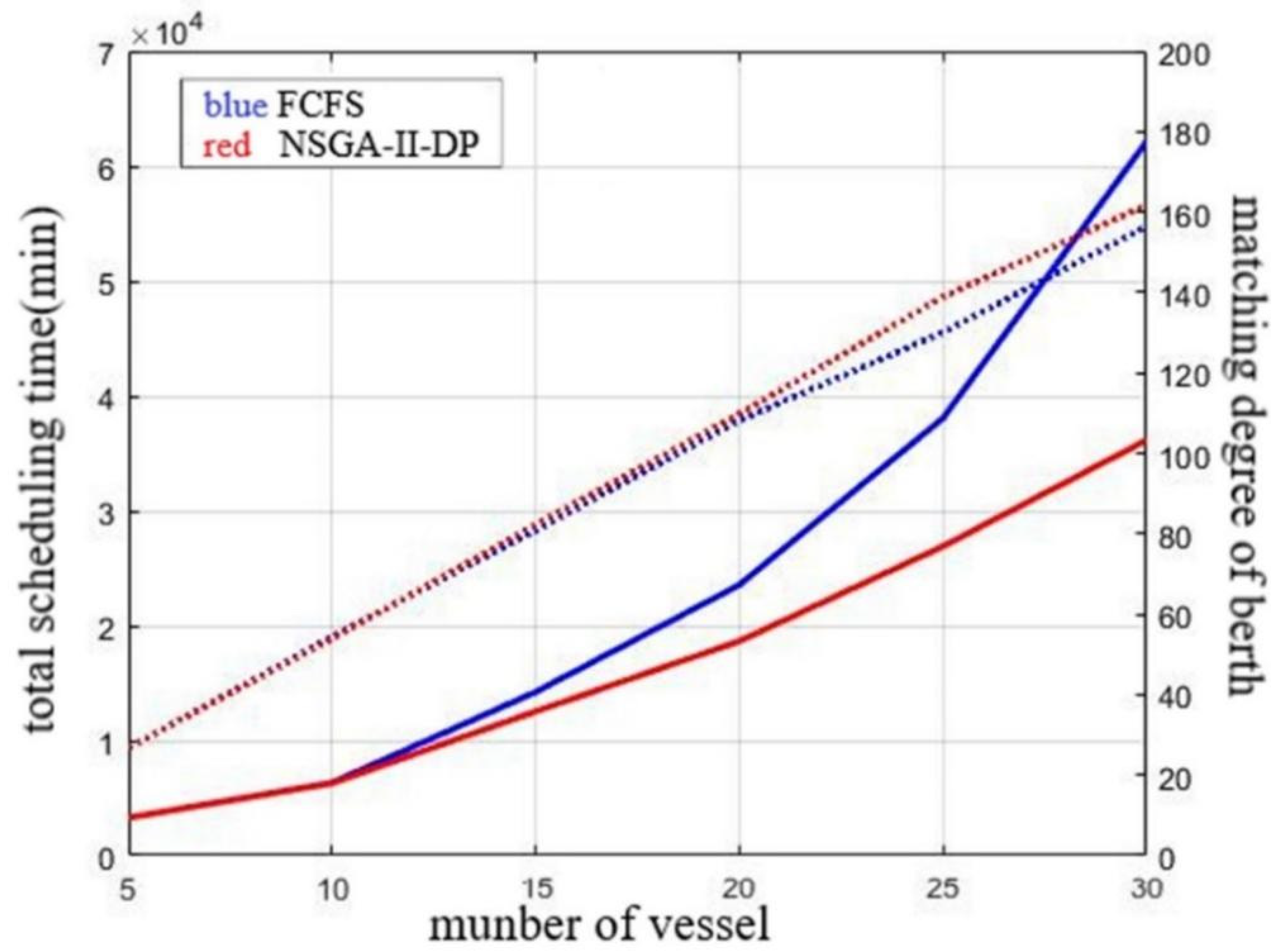
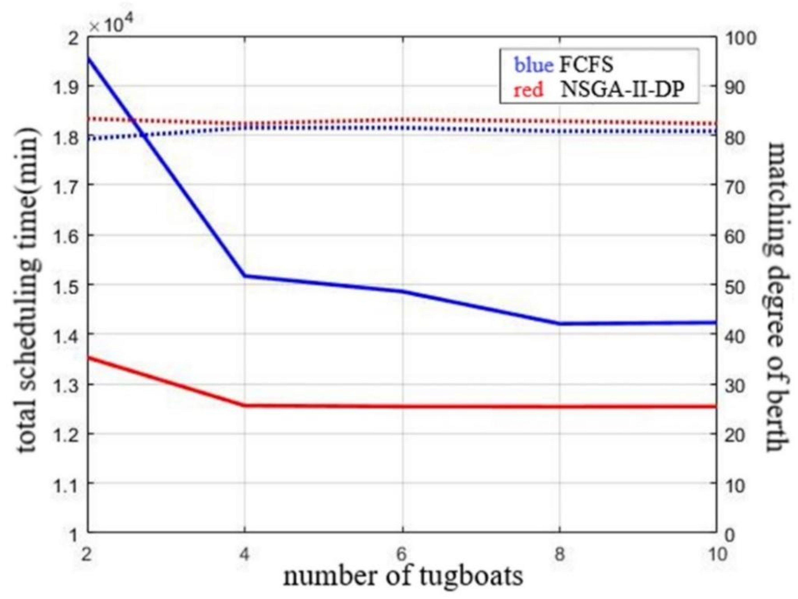
6.3. Sensitivity Analysis
6.4. Sensitivity Analysis
7. Conclusions
- (1)
- By considering both the complex vessel scheduling problem for a restricted channel along with the berth allocation problem, a comprehensive model for vessel scheduling in a restricted channel and berth allocation that considers carbon emissions is developed. avoiding the sub-optimal results of separate optimization.
- (2)
- Tide times, traffic conflicts, port scheduling resources, and other factors are considered in the overall scheduling model to make the model more realistic. Furthermore, the model also considers the matching degree between the berth and the ship and the carbon emissions during navigation, which brings the research more in line with the real requirements of port management and the general trend toward sustainable shipping. Through the experimental results, we explained the relationship between the three objectives, verified the rationality of the model results, and proved the superiority of our model and algorithm compared with the traditional FCFS strategy of port dispatching in different situations.
- (3)
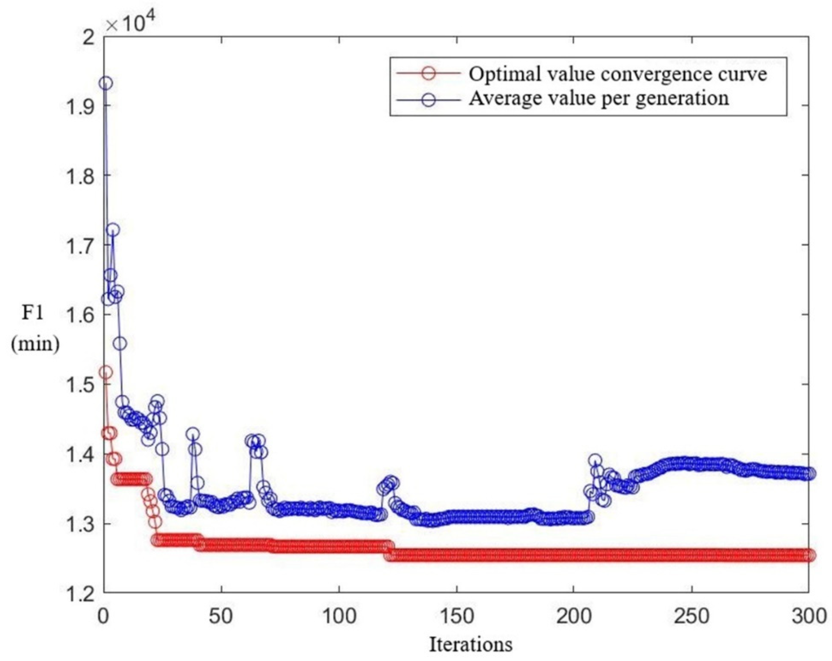
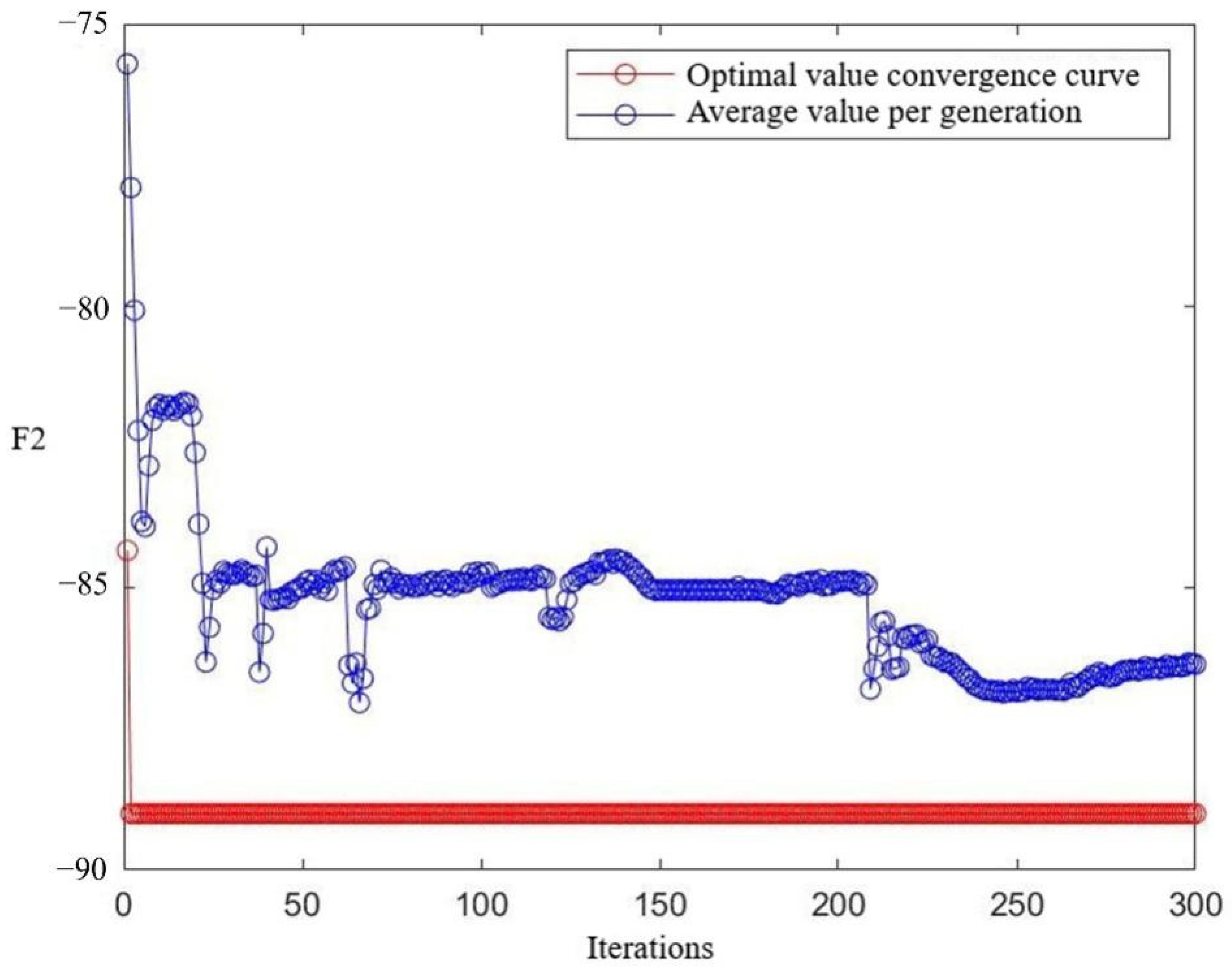
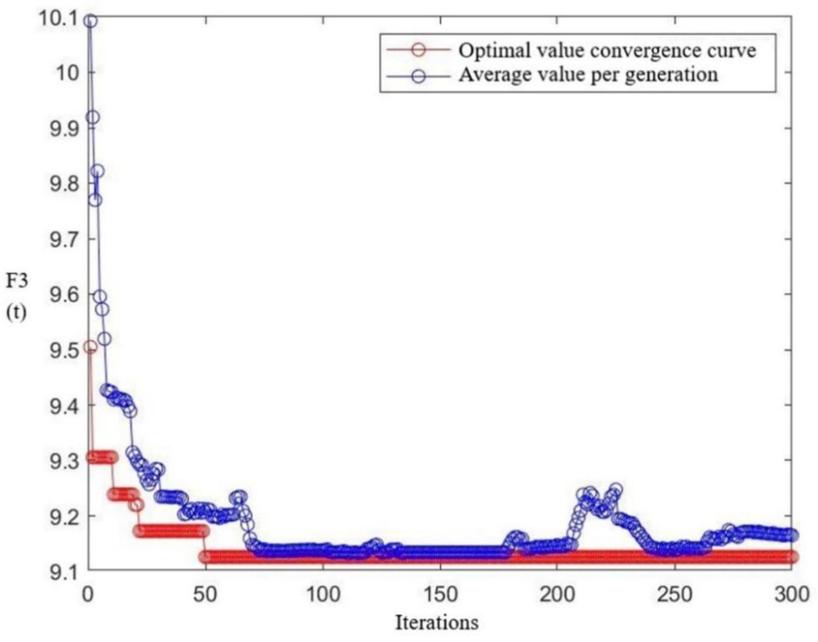
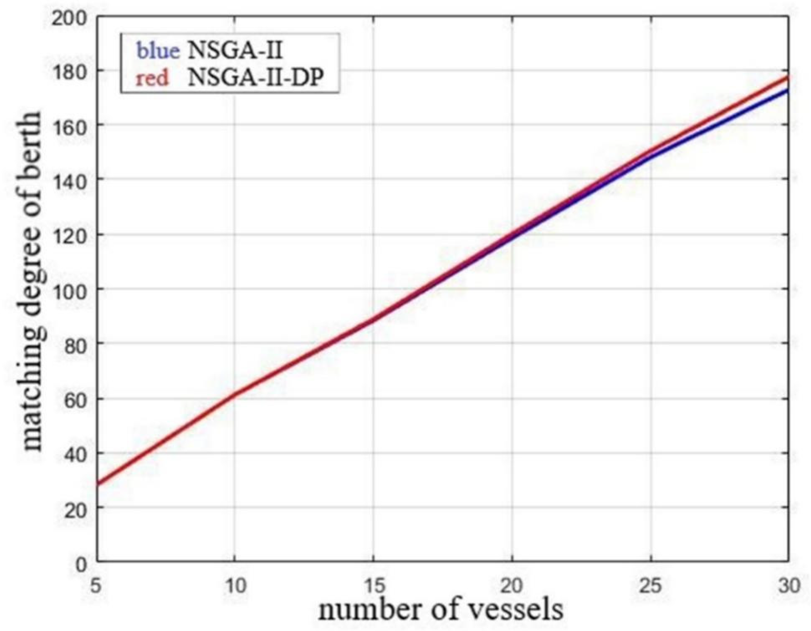
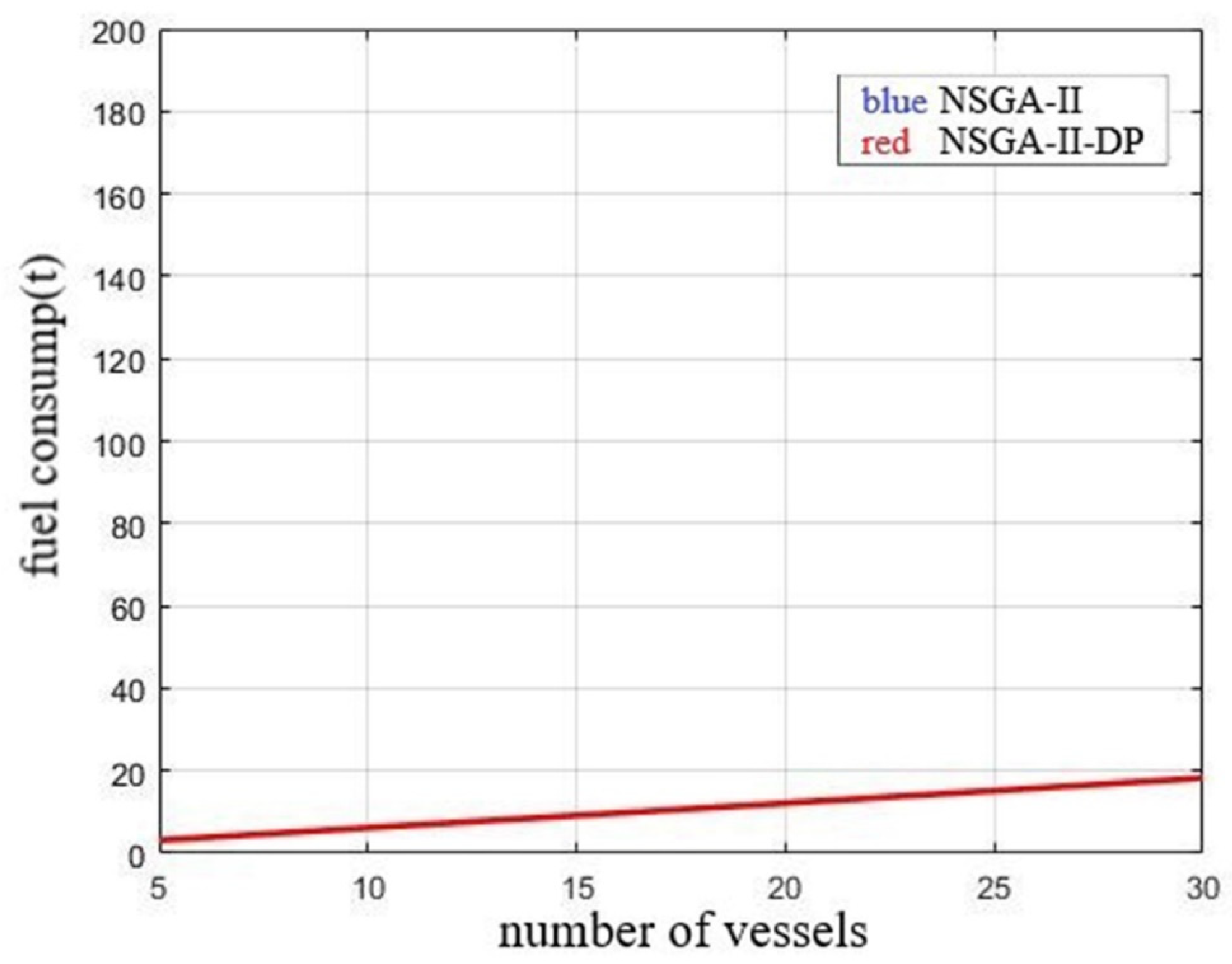
- In order to solve the problem that the population diversity of the NSGA-II algorithm decreases and the solution falls into the local optimum, we have constructed the algorithm NSGA-II-DP. We compared the results of applying the original NSGA-II algorithm and the NSGA-II-DP algorithm to cases with different numbers of vessels. The results showed that the overall convergence of the NSGA-II-DP algorithm is better than that of the NSGA-II algorithm and thus that the proposed NSGA-II-DP algorithm is a successful improvement on the NSGA-II algorithm.
Author Contributions
Funding
Institutional Review Board Statement
Informed Consent Statement
Data Availability Statement
Conflicts of Interest
References
- UNCTAD. Review of Maritime Transport 2021. United Nations Conference on Trade and Development. Available online: https://unctad.org/webflyer/review-maritime-transport-2021 (accessed on 1 October 2022).
- Jia, S.; Li, C.-L.; Xu, Z. Managing navigation channel traffic and anchorage area utilization of a container port. Transp. Sci. 2019, 53, 728–745. [Google Scholar]
- Li, J.; Zhang, X.; Yang, B.; Wang, N. Vessel traffic scheduling optimization for restricted channel in ports. Comput. Ind. Eng. 2021, 152, 107014. [Google Scholar]
- Zhang, X.; Chen, X.; Ji, M.; Yao, S. Vessel scheduling model of a one-way port channel. J. Waterway Port Coast. Ocean. Eng. 2017, 143, 04017009. [Google Scholar]
- Zhang, B.; Zheng, Z. Model and algorithm for vessel scheduling through a one-way tidal channel. J. Waterw. Port Coast. Ocean. Eng. 2020, 146, 04019032. [Google Scholar] [CrossRef]
- Abou Kasm, O.; Diabat, A.; Bierlaire, M. Vessel scheduling with pilotage and tugging considerations. Transp. Res. E. 2021, 148, 102231. [Google Scholar] [CrossRef]
- Hill, A.; Lalla-Ruiz, E.; Voß, S.; Goycoolea, M. A multi-mode resource-constrained project scheduling reformulation for the waterway ship scheduling problem. J. Sched. 2019, 22, 173–182. [Google Scholar]
- Zhang, B.; Zheng, Z.; Wang, D. A model and algorithm for vessel scheduling through a two-way tidal channel. Marit. Policy Manag. 2020, 47, 188–202. [Google Scholar] [CrossRef]
- Lalla-Ruiz, E.; Shi, X.; Voß, S. The waterway ship scheduling problem. Transp. Res. D. 2018, 60, 191–209. [Google Scholar] [CrossRef]
- Zhang, X.; Li, R.; Lin, J.; Xu, C. Optimisation modeling of vessel traffic scheduling for Y shaped bifurcated compound waterway. J. Dalian Marit. Univ. 2018, 44, 1–14. [Google Scholar]
- Al-Refaie, A.; Abedalqader, H. Optimal berth allocation under regular and emergent vessel arrivals. Proc. Inst. Mech. Eng. Part M J. Eng. Marit. Environ. 2021, 235, 642–656. [Google Scholar] [CrossRef]
- Correcher, J.F.; Van den Bossche, T.; Alvarez-Valdes, R.; Vanden Berghe, G. The berth allocation problem in terminals with irregular layouts. Eur. J. Oper. Res. 2019, 272, 1096–1108. [Google Scholar]
- Dulebenets, M.A. An Adaptive Island Evolutionary Algorithm for the berth scheduling problem. Memetic Comput. 2020, 12, 51–72. [Google Scholar]
- Bacalhau, E.T.; Casacio, L.; Tavares de Azevedo, A. New hybrid genetic algorithms to solve dynamic berth allocation problem. Expert Syst. Appl. 2021, 167, 114198. [Google Scholar] [CrossRef]
- Liu, C.; Xiang, X.; Zheng, L. A two-stage robust optimization approach for the berth allocation problem under uncertainty. Flexible Serv. Manuf. J. 2020, 32, 425–452. [Google Scholar]
- Mnasri, S.; Alrashidi, M. A comprehensive modeling of the discrete and dynamic problem of berth allocation in maritime terminals. Electronics 2021, 10, 2684. [Google Scholar]
- Hu, Z.H. Low-emission berth allocation by optimizing sailing speed and mooring time. Transport 2020, 35, 486–499. [Google Scholar]
- Guo, L.; Wang, J.; Zheng, J. Berth allocation problem with uncertain vessel handling times considering weather conditions. Comput. Ind. Eng. 2021, 158, 107417. [Google Scholar] [CrossRef]
- Wu, Y.; Miao, L. An efficient procedure for inserting buffers to generate robust berth plans in container terminals. Discret. Dyn. Nat. Soc. 2021, 2021, 6619538. [Google Scholar] [CrossRef]
- Guo, W.; Ji, M.; Zhu, H. Multi-period coordinated optimization on berth allocation and yard assignment in container terminals based on truck route. IEEE Access 2021, 9, 83124–83136. [Google Scholar]
- Zhang, X.; Lin, J.; Guo, Z.; Liu, T. Vessel transportation scheduling optimization based on channel–berth coordination. Ocean Eng. 2016, 112, 145–152. [Google Scholar] [CrossRef]
- Liu, B.; Li, Z.C.; Sheng, D.; Wang, Y. Short-term berth planning and ship scheduling for a busy seaport with channel restrictions. Transp. Res. E 2021, 154, 102467. [Google Scholar]
- Liu, B.; Li, Z.C.; Sheng, D.; Wang, Y. Integrated planning of berth allocation and vessel sequencing in a seaport with one-way navigation channel. Transp. Res. B Methodol. 2021, 143, 23–47. [Google Scholar]
- Wang, B. Research on Bulk Cargo Port Ship Scheduling System Based on Multi-Objective and Genetic Algorithm. Master’s Thesis, Beijing Jiaotong University, Beijing, China, 2021. (In Chinese). [Google Scholar]
- Al-Hammadi, J.; Diabat, A. An integrated berth allocation and yard assignment problem for bulk ports: Formulation and case study. RAIRO-Oper. Res. 2017, 51, 267–284. [Google Scholar]
- Iris, C.; Lam, J.; Siu, L. Recoverable robustness in weekly berth and quay crane planning. Transp. Res. Part B Methodol. 2019, 122, 365–389. [Google Scholar]
- Iris, C.; Pacino, D.; Ropke, S.; Larsen, A. Integrated berth allocation and quay crane assignment problem: Set partitioning models and computational results. Transp. Res. Part E Logist. Transp. Rev. 2015, 81, 75–97. [Google Scholar]
- Venturini, G.; Iris, C.; Kontovas, C.A.; Larsen, A. The multi-port berth allocation problem with speed optimization and emission considerations. Transp. Res. Part D Transp. Environ. 2017, 54, 142–159. [Google Scholar]
- Coello, C.A.C. An updated survey of GA-based multiobjective optimization techniques. ACM Comput. Surv. 2000, 32, 109–143. [Google Scholar]
- Fonseca, C.M.; Fleming, P.J. Genetic algorithms for multiobjective optimization—Formulation, discussion and generalization. In Proceedings of the Annual Meeting for the 5th International Conference on Genetic Algorithms, University Illinois Urbana Champaign. Urbana, IL, USA, 17–21 July 1993. [Google Scholar]
- Srinivas, N.; Deb, K. Multiobjective function optimization using nondominated sorting genetic algorithms. Evlutionary Comput. 1995, 2, 221–248. [Google Scholar]
- Yu, J.; Yin, Y. Assembly line balancing based on an adaptive genetic algorithm. Int. J. Adv. Manuf. Technol. 2010, 48, 347–354. [Google Scholar] [CrossRef]


| Authors | Research Topic | Channel | Constraint | Objective Function | Algorithm | |||||||||||||||
|---|---|---|---|---|---|---|---|---|---|---|---|---|---|---|---|---|---|---|---|---|
| CSP | BAP | CSP + BAP | 1 | 2 | 3 | 4 | 5 | 6 | 7 | 8 | 9 | 10 | 11 | 12 | 13 | 14 | ||||
| Zhang et al. | √ | one-way | √ | √ | √ | 1 + 2 | GA | |||||||||||||
| Zhang et al. | √ | one-way | √ | √ | 1 | SA + GA | ||||||||||||||
| Kasm et al. | √ | one-way | √ | √ | √ | 3 | CHA | |||||||||||||
| Hill et al. | √ | two-way | √ | √ | √ | 1 | CS | |||||||||||||
| Zhang et al. | √ | two-way | √ | √ | 1 | GA | ||||||||||||||
| Lalla-Ruiz et al. | √ | compound | √ | 1 | SA + TSP | |||||||||||||||
| Zhang et al. | √ | compound | √ | √ | 1 | GA | ||||||||||||||
| Li et al. | √ | restricted | √ | √ | √ | √ | √ | 1 + 2 | GA | |||||||||||
| Abbas et al. | √ | - | √ | √ | √ | √ | √ | 4 | CS | |||||||||||
| Correcher et al. | √ | - | √ | √ | √ | √ | 5 | CHA | ||||||||||||
| Maxim et al. | √ | - | √ | √ | √ | 6 | AIEA | |||||||||||||
| Eduardo et al. | √ | - | √ | √ | √ | √ | √ | 7 | GA + CHA | |||||||||||
| Liu et al. | √ | - | √ | √ | √ | √ | 8 | SWA + CHA | ||||||||||||
| Sami et al. | √ | - | √ | √ | √ | 7 | O-MaSE | |||||||||||||
| Hu et al. | √ | - | √ | √ | √ | √ | 9 + 10 | ε | ||||||||||||
| Guo et al. | √ | - | √ | √ | √ | √ | 11 + 12 | PSO | ||||||||||||
| Wu et al. | √ | - | √ | √ | √ | √ | 13 | CHA | ||||||||||||
| Guo et al. | √ | - | √ | √ | √ | √ | √ | 14 | GA | |||||||||||
| Zhang et al. | √ | one-way | √ | √ | √ | √ | √ | 1 | SA + GA | |||||||||||
| Liu et al. | √ | one-way | √ | √ | √ | √ | √ | √ | √ | 15 | CHA | |||||||||
| Liu et al. | √ | two-way | √ | √ | √ | √ | √ | √ | √ | 16 | CG | |||||||||
| Present study | √ | restricted | √ | √ | √ | √ | √ | √ | √ | √ | √ | √ | √ | √ | 1 + 10 + 17 | GA | ||||
| Type of Vessel | 35000 DWT Bulk Carrier | 35000 DWT Bulk Carrier | 35000 DWT Bulk Carrier |
|---|---|---|---|
| Dead weight (t) | 16,000 | 13,000 | 12,000 |
| Net load weight (t) | 35,000 | 50,000 | 75,000 |
| Vessel length (m) | 190 | 200 | 225 |
| Vessel draft (m) | 10 | 12 | 14 |
| Fuel consumption rate (g/kWh) | 167 | 130 | 127 |
| Berth Number | Water Depth (m) | Length (m) | Types of Cargo Serviced | Center Point Coordinates | Loading and Unloading Speed (t/h) |
|---|---|---|---|---|---|
| Berth 1 | 230 | 15 | ore, steel, coal | (20, 2212) | 4200 |
| Berth 2 | 210 | 13 | coal | (20, 1942) | 4600 |
| Berth 3 | 210 | 13 | coal, ore | (20, 1682) | 4900 |
| Berth 4 | 195 | 11 | ore | (20, 1429.5) | 5200 |
| Berth 5 | 210 | 13 | steel | (205, 1282) | 4600 |
| Berth 6 | 210 | 13 | coal, grain, ore | (465, 1282) | 4300 |
| Berth 7 | 210 | 13 | steel, coal | (725, 1282) | 5300 |
| Berth 8 | 195 | 11 | steel, ore | (910, 1429.5) | 3900 |
| Berth 9 | 195 | 11 | grain, coal | (910, 1674.5) | 5400 |
| Berth 10 | 210 | 13 | grain | (910, 1927) | 4600 |
| Berth 11 | 230 | 15 | grain, ore | (910, 2197) | 3600 |
| Parameter | Distance (nautical miles) |
|---|---|
| 4.4 | |
| 4.1 | |
| 4.2 | |
| 1.25 | |
| 1.85 |
| Vessel Number | Loading or Unloading | Tonnage (t) | Types of Cargo | Serial Number of Stockyard Space Allocated to the Vessel | Coordinates of Central Point of Stockyard Space | Time of Vessel Applying for Inbound Operation (min) | Number of Tugs Required |
|---|---|---|---|---|---|---|---|
| 1 | Unloading | 50,000 | Ore | 14, 49, 8 | (240, 939), (90, 177), (240, 1066) | 0 | 2 |
| 2 | Loading | 50,000 | Ore | 44, 34, 37 | (240, 304), (540, 558), (90, 431) | 11 | 2 |
| 3 | Unloading | 75,000 | Steel | 30, 20, 42, 59 | (840, 685), (240, 812), (840, 431), (690, 50) | 35 | 2 |
| 4 | Unloading | 35,000 | Coal | 5, 45 | (690, 1193), (390, 304) | 120 | 2 |
| 5 | Loading | 35,000 | Coal | 41, 4 | (690, 431), (540, 1193) | 126 | 2 |
| 6 | Unloading | 35,000 | Steel | 1, 2 | (90, 1193), (240, 1193) | 145 | 2 |
| 7 | Unloading | 50,000 | Grain | 12, 26, 54 | (840, 1066), (240, 685), (840, 177) | 170 | 2 |
| 8 | Loading | 50,000 | Grain | 7, 22, 23 | (90, 1066), (540, 812), (690, 812) | 179 | 2 |
| 9 | Loading | 35,000 | Ore | 58, 53 | (540, 50), (690, 177) | 240 | 2 |
| 10 | Unloading | 50,000 | Coal | 36, 28, 33 | (840, 558), (540, 685), (390, 558) | 300 | 2 |
| 11 | Loading | 75,000 | Ore | 60, 52, 6, 29 | (840, 50), (540, 177), (840, 1193), (690, 685) | 332 | 2 |
| 12 | Loading | 50,000 | Grain | 10, 19, 40 | (540, 1066), (90, 812), (540, 413) | 476 | 2 |
| 13 | Unloading | 50,000 | Steel | 35, 17, 25 | (690, 558), (690, 939), (90, 685) | 540 | 2 |
| 14 | Loading | 50,000 | Steel | 11, 39, 43 | (690, 1066), (390, 431), (90, 304) | 641 | 2 |
| 15 | Unloading | 75,000 | Coal | 46, 18, 47, 31 | (540, 304), (840, 939) (690, 304), (90, 558) | 645 | 2 |
| Total Scheduling Time (min) | Berth Matching Degree | Fuel Consumption (t) | |
|---|---|---|---|
| 12,542 | 82.33 | 10.05 | |
| 12,544 | 82.33 | 9.52 | |
| 12,567 | 82.33 | 9.13 | |
| 12,922 | 82.67 | 9.40 | |
| 12,987 | 83.83 | 9.37 | |
| 12,994 | 85.33 | 9.13 | |
| 13,365 | 86 | 9.13 | |
| 13,476 | 86.33 | 9.13 | |
| 13,911 | 87 | 9.22 | |
| 13,913 | 87 | 9.13 | |
| 13,959 | 87.33 | 9.13 | |
| 14,040 | 88.33 | 9.13 | |
| 14,897 | 89 | 9.13 | |
| Optimal value | F1 | F2 | F3 |
| 12,542 | 89 | 9.13 |
| Vessel Number | Start Time of Inbound Operations That Was Applied for (min) | Actual Start Time of Inbound Journey (min) | Start Time of Outbound Operations That Was Applied for (min) | Actual Start Time of Outbound Operations (min) | Allocated Berth | Vessel Speed (Knots) | |
|---|---|---|---|---|---|---|---|
| Channel | Harbor Basin | ||||||
| 1 | 0 | 0 | 613 | 629 | 3 | 8 | 5 |
| 2 | 11 | 15 | 713 | 806 | 6 | 8 | 5 |
| 3 | 35 | 152 | 1224 | 1230 | 1 | 8.9 | 5 |
| 4 | 120 | 120 | 509 | 509 | 9 | 8.7 | 5 |
| 5 | 126 | 135 | 532 | 532 | 7 | 8.7 | 5 |
| 6 | 145 | 193 | 650 | 650 | 5 | 8.7 | 5 |
| 7 | 170 | 170 | 823 | 823 | 10 | 8 | 5 |
| 8 | 179 | 771 | 1424 | 1424 | 10 | 8 | 5 |
| 9 | 240 | 240 | 644 | 665 | 4 | 8.7 | 5 |
| 10 | 300 | 300 | 953 | 953 | 2 | 8 | 5 |
| 11 | 332 | 332 | 1582 | 1582 | 11 | 8.9 | 5 |
| 12 | 476 | 786 | 1484 | 1484 | 6 | 8 | 5 |
| 13 | 540 | 615 | 1268 | 1268 | 5 | 8 | 5 |
| 14 | 641 | 641 | 1208 | 1208 | 7 | 8 | 5 |
| 15 | 645 | 1667 | 2739 | 2739 | 1 | 8.9 | 5 |
| Total vessel scheduling time (min) | Berth matching degree | Fuel consumption (t) | |||||
| 12,542 | 82.33 | 10.05 | |||||
| Vessel Number | Time of Entry to Area A (min) | Time Leaving Area A (min) | Time of Entry to Area B (min) | Time Leaving Area B (min) | Time of Entry to Area C (min) | Time Leaving Area C (min) | ||||||
|---|---|---|---|---|---|---|---|---|---|---|---|---|
| Inbound | Outbound | Inbound | Outbound | Inbound | Outbound | Inbound | Outbound | Inbound | Outbound | Inbound | Outbound | |
| 1 | 33 | 705 | 64 | 736 | 64 | 673 | 96 | 705 | 96 | 629 | 165 | 673 |
| 2 | 48 | 882 | 79 | 913 | 79 | 850 | 111 | 882 | 111 | 806 | 180 | 850 |
| 3 | 182 | 1302 | 210 | 1330 | 210 | 1273 | 239 | 1302 | 239 | 1230 | 327 | 1273 |
| 4 | 151 | 581 | 180 | 610 | 180 | 552 | 209 | 581 | 209 | 509 | 277 | 552 |
| 5 | 166 | 604 | 195 | 633 | 195 | 575 | 224 | 604 | 224 | 532 | 292 | 575 |
| 6 | 224 | 722 | 253 | 751 | 253 | 693 | 282 | 722 | 282 | 650 | 350 | 693 |
| 7 | 203 | 899 | 234 | 930 | 234 | 867 | 266 | 899 | 266 | 823 | 335 | 867 |
| 8 | 804 | 1500 | 835 | 1531 | 835 | 1468 | 867 | 1500 | 867 | 1424 | 936 | 1468 |
| 9 | 271 | 737 | 300 | 766 | 300 | 708 | 329 | 737 | 329 | 665 | 397 | 708 |
| 10 | 333 | 1029 | 364 | 1060 | 364 | 997 | 396 | 1029 | 396 | 953 | 465 | 997 |
| 11 | 362 | 1654 | 390 | 1682 | 390 | 1625 | 419 | 1654 | 419 | 1582 | 487 | 1625 |
| 12 | 819 | 1560 | 850 | 1591 | 850 | 1528 | 882 | 1560 | 882 | 1484 | 951 | 1528 |
| 13 | 648 | 1344 | 679 | 1375 | 679 | 1312 | 711 | 1344 | 711 | 1268 | 780 | 1312 |
| 14 | 674 | 1284 | 705 | 1315 | 705 | 1252 | 737 | 1284 | 737 | 1208 | 806 | 1252 |
| 15 | 1697 | 2811 | 1725 | 2839 | 1725 | 2782 | 1754 | 2811 | 1754 | 2739 | 1822 | 2782 |
| Number of Vessels | NSGA-II-DP | ||
|---|---|---|---|
| Optimal Value of Total Scheduling Time in Pareto Solution Set, F1 (min) | Optimal Value of Berth Matching Degree in Pareto Solution Set, F2 | Optimal Value of Fuel Consumption in Pareto Solution Set, F3 (t) | |
| 5 | 3285 | 28.25 | 3.1202 |
| 10 | 6316 | 61.25 | 6.1631 |
| 15 | 13,146 | 89 | 9.126 |
| 20 | 20,696 | 120 | 12.1289 |
| 25 | 30,649 | 148.25 | 15.1318 |
| 30 | 40,213 | 173.25 | 18.252 |
| Number of Vessels | FCFS | NSGA-II-DP | Gap (%) | |||
|---|---|---|---|---|---|---|
| F1 (min) | F2 | F1 (min) | F2 | |||
| 5 | 3293 | 26.75 | 3285 | 26.75 | −0.24 | 0 |
| 10 | 6334 | 54.42 | 6292 | 53.92 | −0.66 | −0.92 |
| 15 | 14,231 | 80.83 | 12,542 | 82.33 | −11.87 | 1.86 |
| 20 | 23,549 | 108.17 | 18,651 | 109.83 | −20.80 | 1.53 |
| 25 | 38,058 | 130.08 | 26,910 | 138.92 | −29.88 | 6.80 |
| 30 | 62,134 | 156.42 | 36,154 | 161.75 | −41.81 | 3.41 |
| Number of Tugs | FCFS | NSGA-II-DP | Gap (%) | |||
|---|---|---|---|---|---|---|
| F1 (min) | F2 | F1 (min) | F2 | |||
| 2 | 19,572 | 79.25 | 13,532 | 83.33 | −30.86 | 5.15 |
| 4 | 15,169 | 81.5 | 12,561 | 82.33 | −17.20 | 1.01 |
| 6 | 14,857 | 81.5 | 12,543 | 83.17 | −11.87 | 2.04 |
| 8 | 14,208 | 80.83 | 12,539 | 82.83 | −11.74 | 2.49 |
| 10 | 14,231 | 80.83 | 12,542 | 82.33 | −11.87 | 1.86 |
| Number of Vessels | 5 | 10 | 15 | 20 | 25 | 30 | ||
|---|---|---|---|---|---|---|---|---|
| F1: optimal value of total scheduling time (min) | NSGA-II | Worst value in 10 calculations | 3285 | 6358 | 12,962 | 19,896 | 29,506 | 40,393 |
| Best value in 10 calculations | 3285 | 6305 | 12,564 | 18,468 | 27,341 | 36,450 | ||
| Average of 10 calculations | 3285 | 6331.6 | 12,807.1 | 19,211.6 | 28,298.1 | 38,475.3 | ||
| NSGA-II-DP | Worst value in 10 calculations | 3285 | 6353 | 12,913 | 19,566 | 28,211 | 38,913 | |
| Best value in 10 calculations | 3285 | 6292 | 12,542 | 18,651 | 26,910 | 36,154 | ||
| Average value of 10 calculations | 3285 | 6315.8 | 12,723.8 | 19,188.4 | 27,665.3 | 37,188.9 | ||
| F2: optimal value of berth matching degree | NSGA-II | Worst value in 10 calculations | 28.25 | 61.25 | 87.67 | 116.5 | 146.42 | 170.08 |
| Best value in 10 calculations | 28.25 | 61.25 | 89 | 120 | 149.58 | 175.75 | ||
| Average value of 10 calculations | 28.25 | 61.25 | 88.47 | 118.6 | 148.13 | 172.85 | ||
| NSGA-II-DP | Worst value in 10 calculations | 28.25 | 61.25 | 87.67 | 120 | 147.92 | 175.08 | |
| Best value in 10 calculations | 28.25 | 61.25 | 89 | 120 | 150.92 | 178.92 | ||
| Average value of 10 calculations | 28.25 | 61.25 | 88.87 | 120 | 150.42 | 177.60 | ||
| F3: optimal value of fuel consumption (t) | NSGA-II | Worst value in 10 calculations | 3.12 | 6.16 | 9.13 | 12.13 | 15.13 | 18.25 |
| Best value in 10 calculations | 3.12 | 6.16 | 9.13 | 12.13 | 15.13 | 18.25 | ||
| Average value of 10 calculations | 3.12 | 6.16 | 9.13 | 12.13 | 15.13 | 18.25 | ||
| NSGA-II-DP | Worst value in 10 calculations | 3.12 | 6.16 | 9.13 | 12.13 | 15.13 | 18.25 | |
| Best value in 10 calculations | 3.12 | 6.16 | 9.13 | 12.13 | 15.13 | 18.25 | ||
| Average value of 10 calculations | 3.12 | 6.16 | 9.13 | 12.13 | 15.13 | 18.25 | ||
Publisher’s Note: MDPI stays neutral with regard to jurisdictional claims in published maps and institutional affiliations. |
© 2022 by the authors. Licensee MDPI, Basel, Switzerland. This article is an open access article distributed under the terms and conditions of the Creative Commons Attribution (CC BY) license (https://creativecommons.org/licenses/by/4.0/).
Share and Cite
Jiang, X.; Zhong, M.; Shi, J.; Li, W.; Sui, Y.; Dou, Y. Overall Scheduling Model for Vessels Scheduling and Berth Allocation for Ports with Restricted Channels That Considers Carbon Emissions. J. Mar. Sci. Eng. 2022, 10, 1757. https://doi.org/10.3390/jmse10111757
Jiang X, Zhong M, Shi J, Li W, Sui Y, Dou Y. Overall Scheduling Model for Vessels Scheduling and Berth Allocation for Ports with Restricted Channels That Considers Carbon Emissions. Journal of Marine Science and Engineering. 2022; 10(11):1757. https://doi.org/10.3390/jmse10111757
Chicago/Turabian StyleJiang, Xing, Ming Zhong, Jiahui Shi, Weifeng Li, Yi Sui, and Yuzhi Dou. 2022. "Overall Scheduling Model for Vessels Scheduling and Berth Allocation for Ports with Restricted Channels That Considers Carbon Emissions" Journal of Marine Science and Engineering 10, no. 11: 1757. https://doi.org/10.3390/jmse10111757
APA StyleJiang, X., Zhong, M., Shi, J., Li, W., Sui, Y., & Dou, Y. (2022). Overall Scheduling Model for Vessels Scheduling and Berth Allocation for Ports with Restricted Channels That Considers Carbon Emissions. Journal of Marine Science and Engineering, 10(11), 1757. https://doi.org/10.3390/jmse10111757