AIS-Enabled Weather Routing for Cargo Loss Prevention

Abstract

The operation of any vessel includes risks, such as mechanical failure, collision, property loss, cargo loss, or damage. For modern container ships, safe navigation is challenging as the rate of innovation regarding design, speed profiles, and carrying capacity has experienced exponential growth over the past few years. Prevention of cargo loss in container ship liners is of high importance for the Maritime industry and the waterborne sector as it can lead to potentially disastrous, harmful, or even life-threatening outcomes for the crew, the shipping company, the marine environment, and aqua-culture. With the installment of onboard decision support system(s) (DSS) that will provide the required operational guidance to the vessel’s master, we aim to prevent and overcome such events. This paper explores cargo losses in container ships by employing a novel weather routing optimization DS framework that aims to identify excessive motions and accelerations caused by bad weather at specific times and locations; it also suggests alternative routes and, thus, ultimately prevents cargo loss and damage.

1. Introduction

Optimal ocean route planning is strongly connected to the safety and energy consumption of vessels as well as to the minimization of CO₂ emissions that reduce cost and the overall environmental footprint of shipping. Among other factors, it depends on efficient and robust ship tracking and weather forecasting. There exists a wealth of spatiotemporal data-driven solutions related to these issues that build upon a multitude of features from vessel tracking devices and structural properties of ships, weather conditions, and internal machinery sensors. Tracking can be performed using synthetic aperture radar (SAR) images and data from an automatic identification system (AIS) [1] or other surveillance systems [2]. The spatial dimensions focus on local conditions, e.g., wave-energy spectra and currents, which affect the costs of the overseas movement of a ship, while the temporal aspects correspond to environmental and ship-system conditions, and examine how they evolve with time (e.g., speed, power absorbed by the ship propulsion system, rotational motions along the three axes of the vessel).

Over the past few years, a high rate of innovation was observed concerning the designs (size increase, speed profile, cargo stored on deck) and operational profiles (loading profile, estimated time of arrival, charter party contracts) of container ship liners. This has led to increased risks for Maritime companies as they have little to no experience when it comes to safe and cost-efficient navigation of large, newly-built vessels. Container-carrying capacity has increased by around 1500% since 1968 and has almost doubled in the past decade (this is indicative of the innovation and scale expansion rate). While serious shipping accidents worldwide have declined, incidents involving large vessels—namely container ships—are resulting in disproportionately high losses. Large container ships are prone to onboard accidents and cargo losses due to excessive motions and accelerations in bad weather conditions, leading to environmental pollution and financial damages for Maritime and insurance companies following container loss claims. Parametric roll due to bad weather conditions is one of the main reasons for cargo losses in container ships. Such situations can be avoided if identified along a vessel’s course; these situations can be potentially prevented by employing a decision support (DS) toolkit, which offers the vessel’s master an alternative route that takes into account the weather forecasts, the profile of the vessel, as well as navigational standards.

The research conducted in this paper is supported, enhanced, and validated by a large Maritime company 1 operating more than 70 container ships of various sizes, with a long-term commitment and expertise on the subject of safe navigation. Coupling and incorporating their input with guidelines extracted from the International Maritime Organisation (IMO) regulatory framework, this paper introduces a consolidated approach for routing optimization based on historical AIS and weather data in order to prevent parametric roll of the vessel and, therefore, container loss and damage. The envisaged framework will assist shipowners in achieving efficiency in fleet management with tangible benefits in terms of environmental compliance and protection of cargo and crew safety.

The remainder of the paper is organized as follows. Section 2 presents work related to weather routing. Section 3 provides the methodology followed in this work, including the necessary preprocessing for route extraction (Section 3.1), handling adverse conditions (Section 3.2), and the weather routing algorithm (Section 3.3). Section 4 presents the results of the corresponding computational study, while Section 5 concludes the paper.

2. Related Work

Weather routing has received increased attention in recent years due to increased available computational power, the improved quality of weather data and predictions, the increased interest in autonomous vessels and the drive to reduce emissions from ships. To that end, nowadays there is much better information on weather forecasts, with much higher spatial and temporal resolutions. The improvements in data quality and availability have facilitated the development of online algorithms for optimal routes during voyages. One must consider finding the optimal route and sailing speed for a given voyage considering the environmental conditions, mainly involving wind and waves. The objectives typically involve minimizing operating costs, travel time, fuel consumption, and risk of passage ([3]), with a focus on safety (i.e., parametric rolling or surf riding), comfort (passengers seasickness), and reducing cargo loss and damage. In [4], Fabbri et al. considered navigation risk based on sailing conditions following the IMO guidelines for navigators 2. Moreover, other approaches have targeted multiple objectives [5,6].

Walther et al. [7] evaluated different modeling approaches, optimization algorithms, and their applications in weather routing systems. The analysis shows that the weather routing problem is treated as a single-objective or multi-objective optimization problem that can be modeled as a constrained graph problem, a constrained nonlinear optimization problem, or a combination of both. Depending on the modeling approach, different methods were used to solve it, ranging from Dijkstra’s algorithm [8], dynamic programming [9,10], calculus of variations [11], and optimal control methods, to isochrone methods or iterative approaches for solving nonlinear optimization problems.

Zis et al. [3] presented a taxonomy of weather routing and voyage optimization research in Maritime transportation, explaining the main methodological approaches and key disciplines. Apart from the aforementioned methodologies, the use of pathfinding algorithms and heuristics as well as more recent applications using artificial intelligence and machine learning technologies were included.

Delitala et al. [12] presented two climatological simulations for ship routing. Simulations represented two theoretical long-distance routes in the central–eastern Mediterranean, which were analyzed across various simulated climatic conditions; the results were compared with those of control routes. Furthermore, a route simulator was developed for 7 Mediterranean routes and 15 different ships: passenger, cargo, and RO-PAX (i.e., dedicated to carry both passengers and tracks). The results were analyzed in terms of passenger and crew comfort, bunker consumption by ships, and crossing time. The route simulator, based on the available wind and wave forecasts, takes into account the optimal velocity, corresponding to the desired arrival time, the optimal power, corresponding to the expected fuel consumption, and the minimum comfort index, corresponding to the best possible comfort conditions for passengers.

Shigunov et al. [13] presented some considerations regarding ship-specific operational guidance in order to avoid cargo loss and damage due to conditions of excessive roll motions and large accelerations in heavy weather. Furthermore, limiting values were defined, taking into account the actual lashing systems and mass distributions in container stacks, as well as the standards for probabilistic safety criteria on the basis of the required safety level and cost–benefit considerations. Maki et al. [14] presented a genetic weather routing algorithm that incorporated three different types of objective functions with different weights to balance between fuel efficiency and ship safety, taking into account parametric rolling, and numerically validating that there is a trade-off between ship safety and fuel efficiency.

Veneti et al. [5] proposed a weather routing algorithm based on an exact time-dependent bi-objective shortest path algorithm for ship routes in the area of the Aegean Sea, Greece. The two objectives of the problem involved the minimization of fuel consumption and the total risk of the ship route while taking into account the prevailing weather conditions and the total travel time. In the proposed model, the risk was defined as the combination of the results of a marine accident probability with the severity of its consequences. These accidents can be divided into nine categories: foundered, missing vessel, fire/explosion, collision, contact, grounding/wrecked/stranded, war loss/hostilities, hull/machinery damage, and miscellaneous. For the risk assessment information, such as the vessel type, size, age, flag, navigation area characteristics, traffic data, and historic data about accidents, weather and sea conditions were considered.

Perera et al. [15] presented an overview of weather routing and safe ship handling approaches in the shipping industry, which should be implemented simultaneously to achieve optimal and safe ship navigation conditions and minimize the respective environmental pollution. In particular, weather routing and safe ship handling were combined by selecting an optimal route with appropriate ship orientations and engine power configurations with vessel design characteristics under forecasted and actual weather conditions (i.e., wind, waves and tides/currents).

In July 2002, Regulation 19 of the International Convention for the Safety of Life at Sea (SOLAS-V) came into force, i.e., large cargo vessels were obliged to fit and use AIS for reporting their position, speed, and heading, and for serving surveillance purposes. This regulation resulted in an abundance of data that completely changed the Maritime surveillance scenario ([16]). Since then, there have been vast amounts of data on the sailing speeds and positions of ships globally. AIS data can be particularly useful to identify when ships deviate due to weather from traditional routes and provide real information on the actual benefits achieved through weather routing, particularly regarding savings in total voyage time.

AIS data are extensively utilized to examine and predict vessel trajectories. In this regard, a dual linear autoencoder approach for vessel trajectory prediction using AIS data was proposed in [17]. Chen et al. [18] proposed a ship movement classification based on AID data using convolutional neural networks. Volkova et al. [19] also utilized neural networks based on AIS data to predict a vessel’s trajectory to reduce the likelihood of collisions or other incidents. A data mining approach was proposed by Rong et al. [20] to characterize shipping routes and offer anomaly detection, while pattern recognition for the vessel’s handling behavior using an AIS sub-trajectory clustering analysis was proposed in [21].

Further, Varlamis et al. [22] presented a methodology for extracting information from the navigation network for an area, using data from the trajectories of multiple vessels, which are collected using AIS. The resulting information was modeled using a network abstraction, which allows identifying the various movement patterns of vessels across an edge of the network and can be the basis for outlying behavior detection using off-the-shelf methods.

Kontopoulos et al. [16] extended the concept of the network abstraction model proposed in [22] and presented a distributed framework that captured the cargo vessel’s behavior and extracted the pattern of its movement using AIS data. Specifically, it employs sparse historic AIS data and polynomial interpolation in order to extract shipping lanes. It modifies a well-established clustering algorithm, called density-based spatial clustering of applications with noise (DBSCAN) in order to achieve more coherent trajectory clusters, which are then composed to create the shipping lanes. Each itinerary that is represented as a set of convex hulls manages to accurately represent the spatial boundaries of the vessel movement indicating that any future AIS position can be effectively predicted and placed in a certain geographic region. Simultaneously, the convex hulls represent the behaviors of the vessel movements in terms of speed and headings and detect possible anomalies and deviations. This Maritime traffic model assumes that large vessels of the same type, such as cargo vessels or passenger ships, which mainly employ AIS, travel between the same waypoints by following the same routes and similar speeds, locations, and directions.

Kim et al. [23] calculated the energy efficiency operational indicator (EEOI) for monitoring the operational efficiency of a ship by using big data technologies to handle the large amount of ship dynamic data, which can be obtained from AIS in combination with the ship’s static data and weather data. The latter is used for the estimation of additional resistance acting on the ship in order to calculate the engine power of the ship.

Kaklis et al. [24] presented a big data framework for the real-time monitoring of the operational state of a vessel as well as for simulation and model deployment purposes. This tool was utilized accordingly to extend and enhance the methodology initially proposed in [25,26] regarding fuel oil consumption (FOC) estimation. More specifically, a novel recurrent neural network architecture was introduced that ideally approximates the underlying function describing the vessel’s FOC by taking into account historical operational and weather data. Finally, it was demonstrated how the FOC deep learning model could be coupled with a weather routing algorithm, proposing the optimal route for a vessel in terms of fuel consumption efficiency.

The scope of this work is to define a weather routing approach as a decision-making process to select the optimal route in a given voyage, taking into account the expected weather and sea conditions in order to prevent cargo loss and damage in container ships utilizing AIS data. The optimality of the selected route depends on the objective of reducing risk by avoiding certain areas with adverse weather. For this reason, we set some boundaries (standards) for unacceptable combinations of ship speed and course with respect to the mean wave direction, mean seaway periods, and significant wave heights. In order for the ship master to avoid these combinations, an alternative route was proposed in real time to satisfy the standards calculated from the ship’s dynamic data (AIS) and weather data.

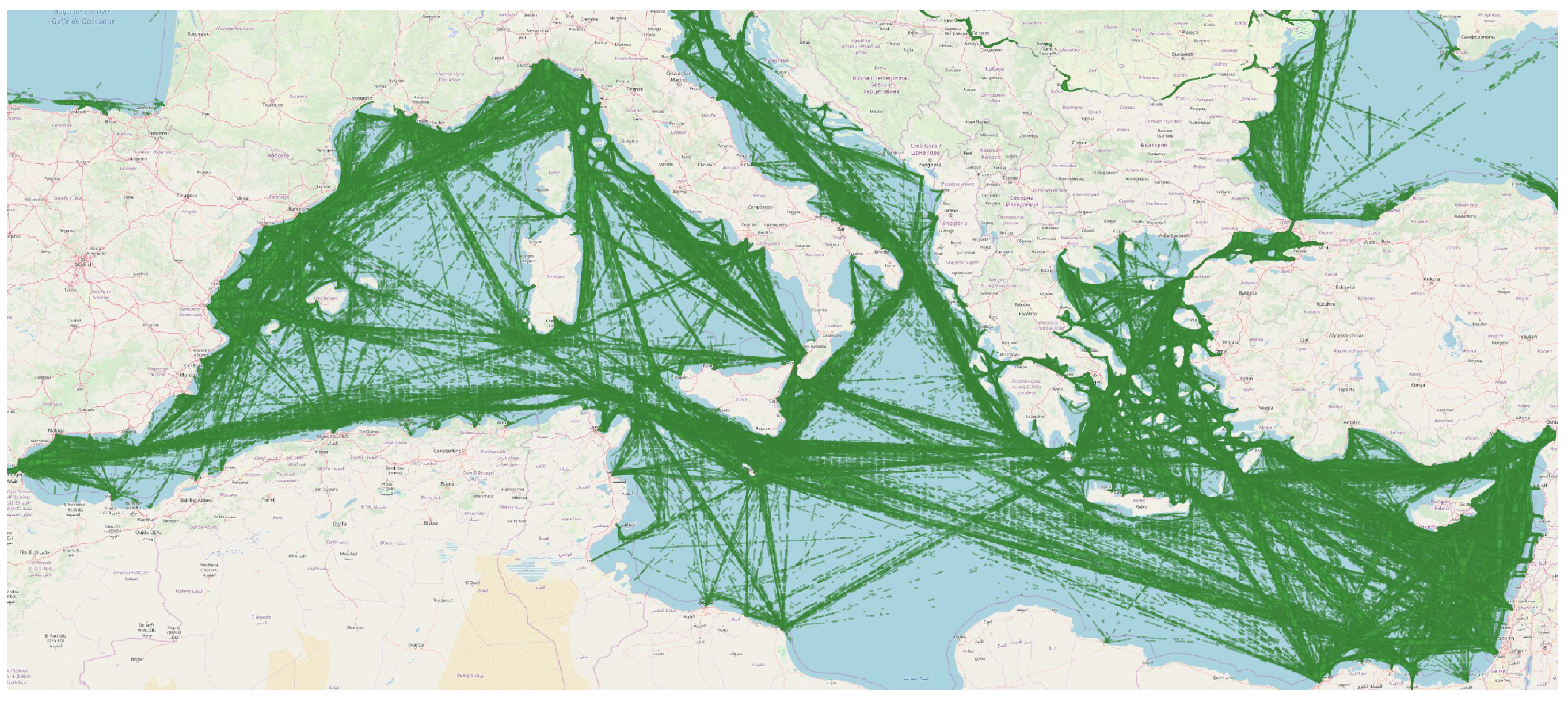
3. Methodology

In this section, a detailed description of the weather routing methodology is provided. Initially, a preprocessing phase takes place to extract the routes from the AIS messages. Then, the proper thresholds of the weather conditions when following Maritime routes are investigated and, finally, the weather routing algorithm is described.

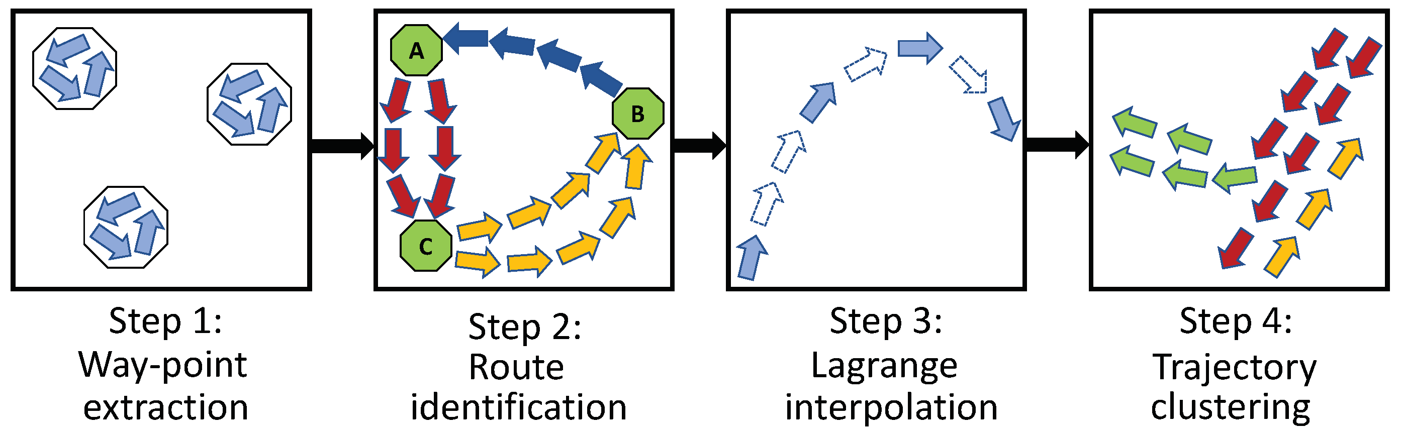
3.1. Preprocessing

In this first phase, Maritime routes need to be extracted to be used as the baseline. To do so, previous works on extracting Maritime traffic patterns [16,22] were exploited. In these works, a series of steps were followed to extract the most commonly used vessel routes. Figure 1 illustrates these steps.

Initially, the DBSCAN clustering algorithm was used to identify clusters or regions at sea, called waypoints, where the vessels stop. These waypoints correspond to ports and anchorage areas. Then, the AIS trajectories of each vessel were segmented based on the waypoints, thus routes from waypoint to waypoint were identified for each vessel. Because the vessel trajectories may be more sparse at certain points in time and space due to bad signal reception or other factors, interpolation was applied to the trajectories in step 3. Therefore, for each vessel route, dense and rich information trajectories were available. The final step employed a modified version of the DBSCAN algorithm to cluster multi-vessel trajectories of the same route (waypoint to waypoint) based on the location, speed, and heading of the AIS positions. As a result, several clusters along each route were created; each cluster represented the area in which vessels moved with a certain speed and heading. More details can be found in [16].

Figure 2 illustrates the final Maritime route network of the Mediterranean Sea that was extracted from the preprocessing phase. For each departure and destination point (e.g., from Piraeus to Port Said), a set of clusters and their centroids are available, which specify the ways the vessels move in terms of space, speed, and headings between the departure and destination points.

3.2. Adverse Weather Conditions for Container Ships

To identify changes in the route based on the weather, the Copernicus Marine Service 3 (CMEMS) and the Copernicus Climate Change Service 4 (C3S) were used for the wave and wind data, respectively. Data from these services are gridded, meaning that weather data are provided for each cell in the grid. The grid resolution for the former service is $0.{083}^{\circ }$, while for the latter service is $0.{25}^{\circ }$. To create a uniform grid for all the weather data at the same time, bilinear interpolation of the wind data onto the wave data was employed. As a result, the final weather grid that contains both wind and wave information had a resolution of $0.{083}^{\circ }$. This resolution was chosen in order to have a more fine-grained grid, creating a richer pool of spatial options to choose from when considering alternate routes. Due to a large amount of weather data for our study area, a three-hourly temporal resolution was chosen. So, each route was generalized and divided into three-hourly intervals to synchronize with the weather data. In particular, the timestamp of each route’s centroid was matched to the nearest available timestamp of the weather data grid.

After careful examination of the IMO guidelines 5${}^{,}$6, the literature review conducted in Section 2 and incorporating the expertise of a major container ship operator (Danaos Shipping), it was decided that the significant wave height, the mean wave period, the mean wind speed, the wave direction, and their corresponding thresholds—adverse condition thresholds—as shown in

Table 1. Weather thresholds of adverse conditions.

Significant Wave Height ${\mathit{h}}_{\mathit{s}}$ (m)	Peak Wave Period ${\mathit{T}}_{\mathit{p}}$ (s)	Mean Wind Speed (m/s) ${\mathit{V}}_{\mathit{w}}$	Wave Direction (Range in ${}^{\circ }$)
≤6.0	$7.0\le T_p\le 15.0$	≤22.6	60–120° and 240–300°

, will be used for the implementation of the weather routing algorithm. Danaos’s expertise originated from the investigation of operational incidents resulting in cargo loss. Investigation reports include weather conditions at the time of the incident as potential root causes for the loss of cargo. The definition of the Weather threshold contains an empirical analysis in reference to the investigation of past incidents as reported in the organizational assets of Danaos shipping.

Specifically, regarding the wave period, it was decided to use the metric of the mean wave period. According to IMO guidelines, when a ship rides on the wave crest, there is a great possibility of its stability reduction. This may become critical for wavelengths ($\lambda$) within the range of 0.6 to 2.3 L (where L is the ship’s length in meters). So, considering the wavelength as 0.6 L, the mean wave period was calculated in relation to the wavelength ($\lambda$) following the equation $0.8·sqrt(\lambda$).

Regarding the wave direction, thresholds according to [13] were used, in which unacceptable combinations of the ship heading, with respect to the mean wave direction, are displayed. If the ship master avoids the lateral wave direction (beam-to-quartering waves) as shown in Table 1, the risk of excessive motions and accelerations will reduce and, thus, the prevention of cargo loss and damage increases.

Our study focused on vessels that have lengths below 200 m (i.e., with the length between perpendiculars (lpp): lpp < 200). This means that at any given time point: (i) the wave must not exceed a height of $4.5$ m, (ii) the mean wave period must not exceed 8 s, (iii) the wind must not exceed a mean speed of 19 m per second, and (iv) the difference between the direction of the wave and the direction of the vessel must not be in the specified ranges.

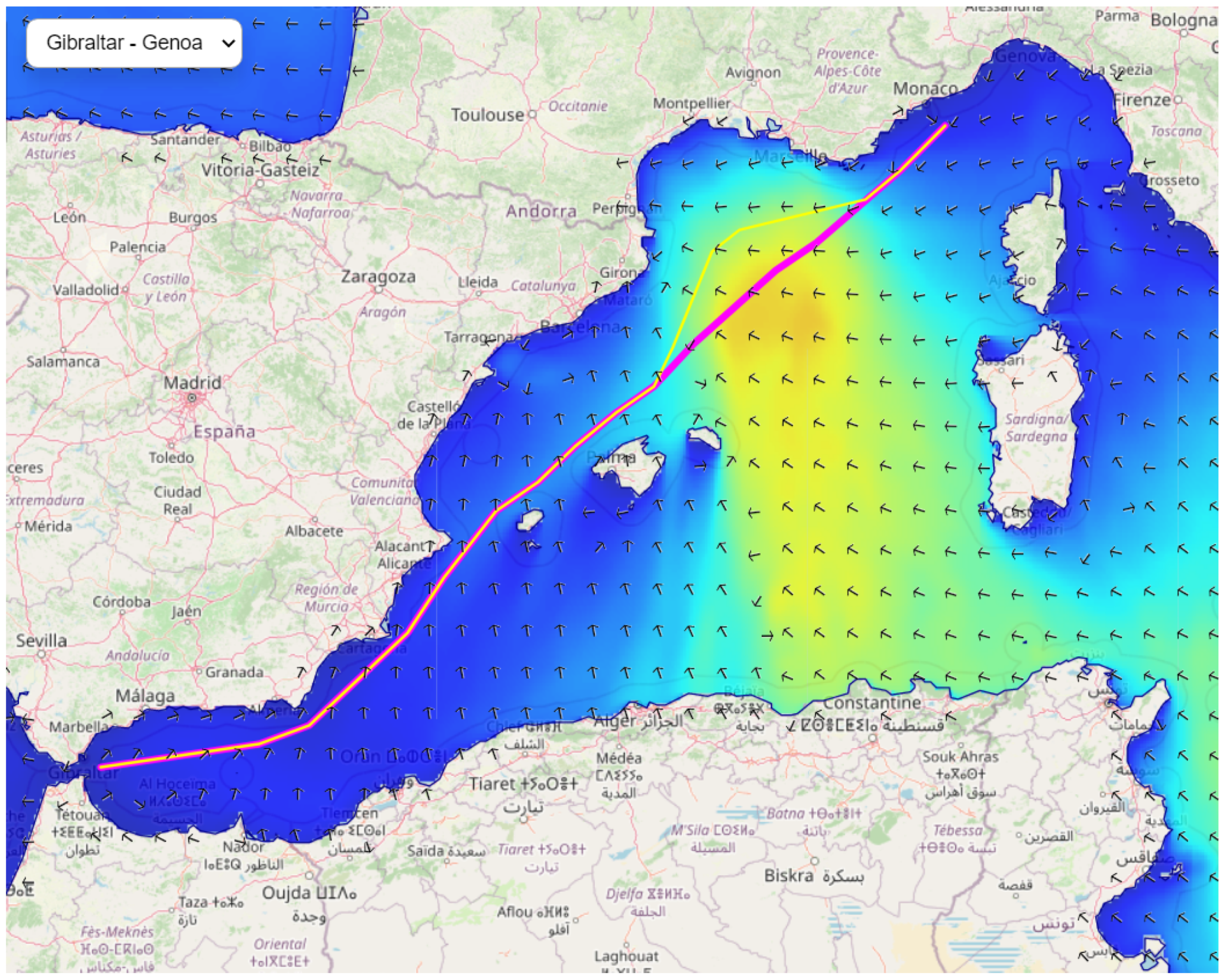
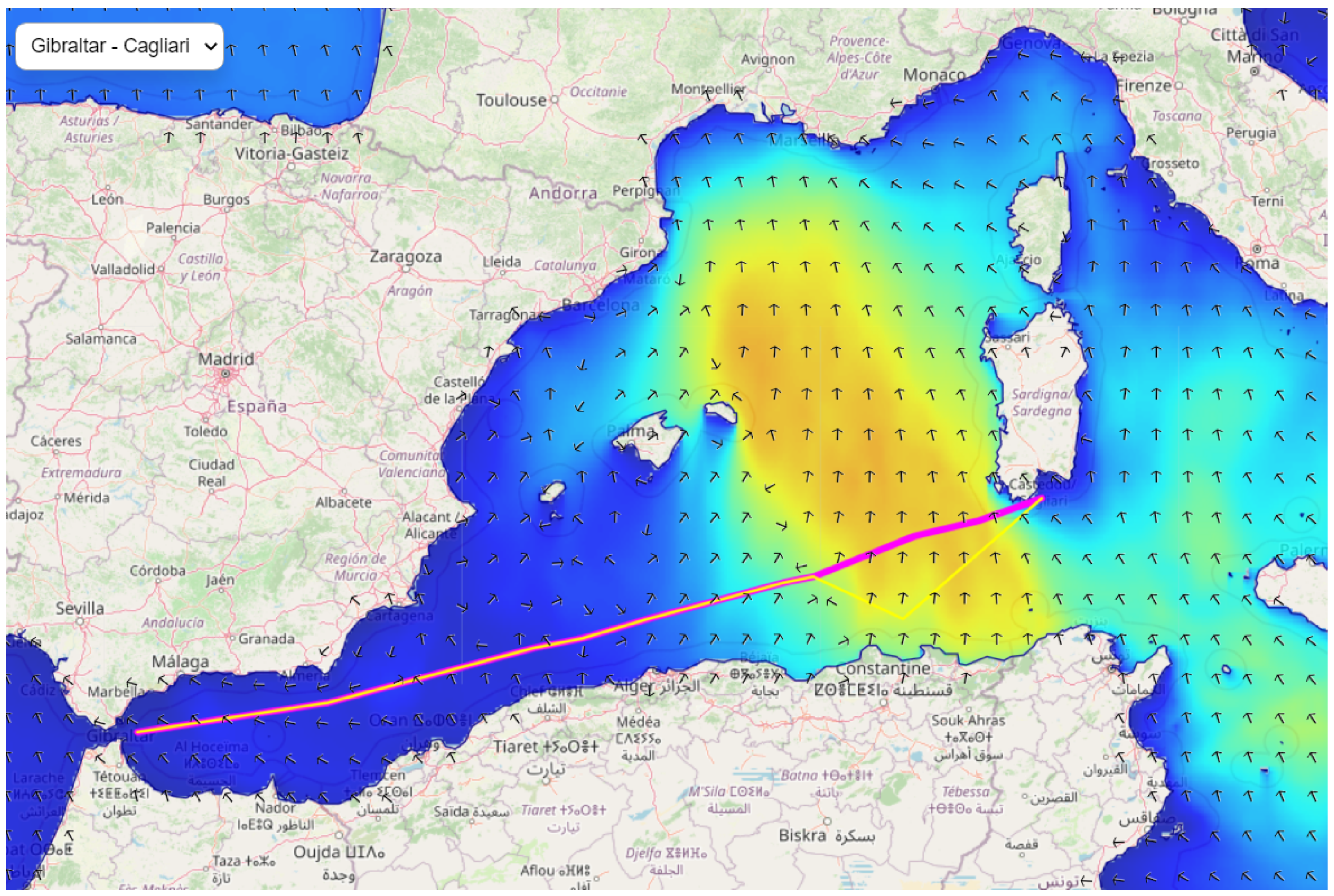
3.3. Weather Routing Algorithm

To calculate an alternate route option based on the adverse weather conditions as defined in Table 1, and given an initial departure/destination point, and departure time, the set of centroids (see Section 3.1) along that route is iterated. The following steps are made during the weather routing process and are depicted in Algorithm 1:

• Based on the current timestamp 7, the mean speed provided by the current centroid of the route 8, and the Haversine 9 distance between the current centroid and the next one along that route, the timestamp of the next centroid is calculated (line 4).
• The position of the next centroid is used to find the cell of the weather grid at which the vessel will be located.
• Given the timestamp and the grid cell of the next centroid, the weather conditions from the Copernicus services are retrieved (line 5).
• If the weather conditions are adverse (see Section 3.2), the nearest cell of the weather grid in the space–time that satisfies the weather thresholds is found (line 7). The centroid of the weather grid acts as the proposed alternative for the vessel to move to (line 8). If the weather conditions are not adverse, the initial centroid is used for the route (line 10). To speed up the process, the search space is limited to the distance the vessel would have traveled, given the mean speed of the centroid and the three-hour time horizon. To find the nearest cell, the nearest neighbor algorithm is employed, which finds the nearest cell in relation to distance from the route centroid using spatial indexing (R-tree). R-trees allow indexing data values, which are defined in two (or more) dimensions. The search strategy uses the best-first-search to query the index, where the values are provided in order of the increasing distance. We limited the search to a maximum of 10 nearest points.
• Finally, the next centroid of the initial route is considered the current one and the entire process repeats itself until there are no more centroids along the route.

Algorithm 1 Weather Routing algorithm
	Input: A set of centroids along the initial route R, Weather Thresholds $WT$
	Output: A set of centroids along the optimized route $R_o$
1:	functionRouteOptimization($R\left[\right]$)
2:	$R_o$ ← $\left[\right]$
3:	for $i\leftarrow 1$ to $length\left(R\right)$ do
4:	$t\left(c_{i+1}\right)$ ← $distance(c_i,c_{i+1})/v\left(c_i\right)$
5:	w←$getWeatherConditions(t\left(c_{i+1}\right),cell\left(c_{i+1}\right))$
6:	if $wexceedsWT$ then
7:	$cellCentroid$ ← $getNearestNeighbor\left(cell\left(c_{i+1}\right)\right)$
8:	${\mathit{R}}_{\mathit{o}}.\mathit{append}\left(\mathit{cellCentroid}\right)$
9:	else
10:	${\mathit{R}}_{\mathit{o}}.\mathit{append}\left({\mathit{c}}_{\mathit{i}+\mathit{1}}\right)$
11:	return $R_o$

Figure 3, Figure 4 and Figure 5 illustrate three examples of the alternate route recommendation via the weather routing algorithm and the adverse condition thresholds. The red lines indicate the initial route the vessel is supposed to follow and the yellow lines indicate the route proposed by the algorithm.

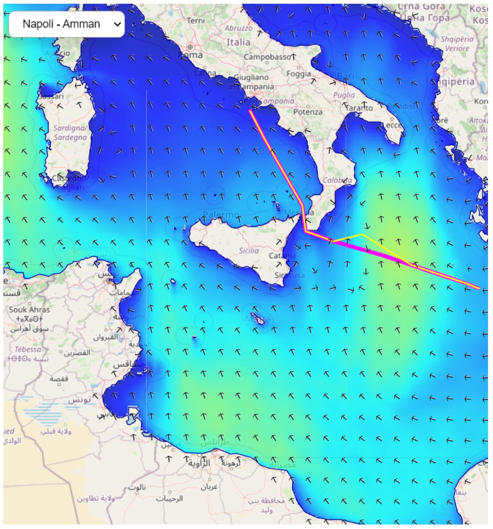
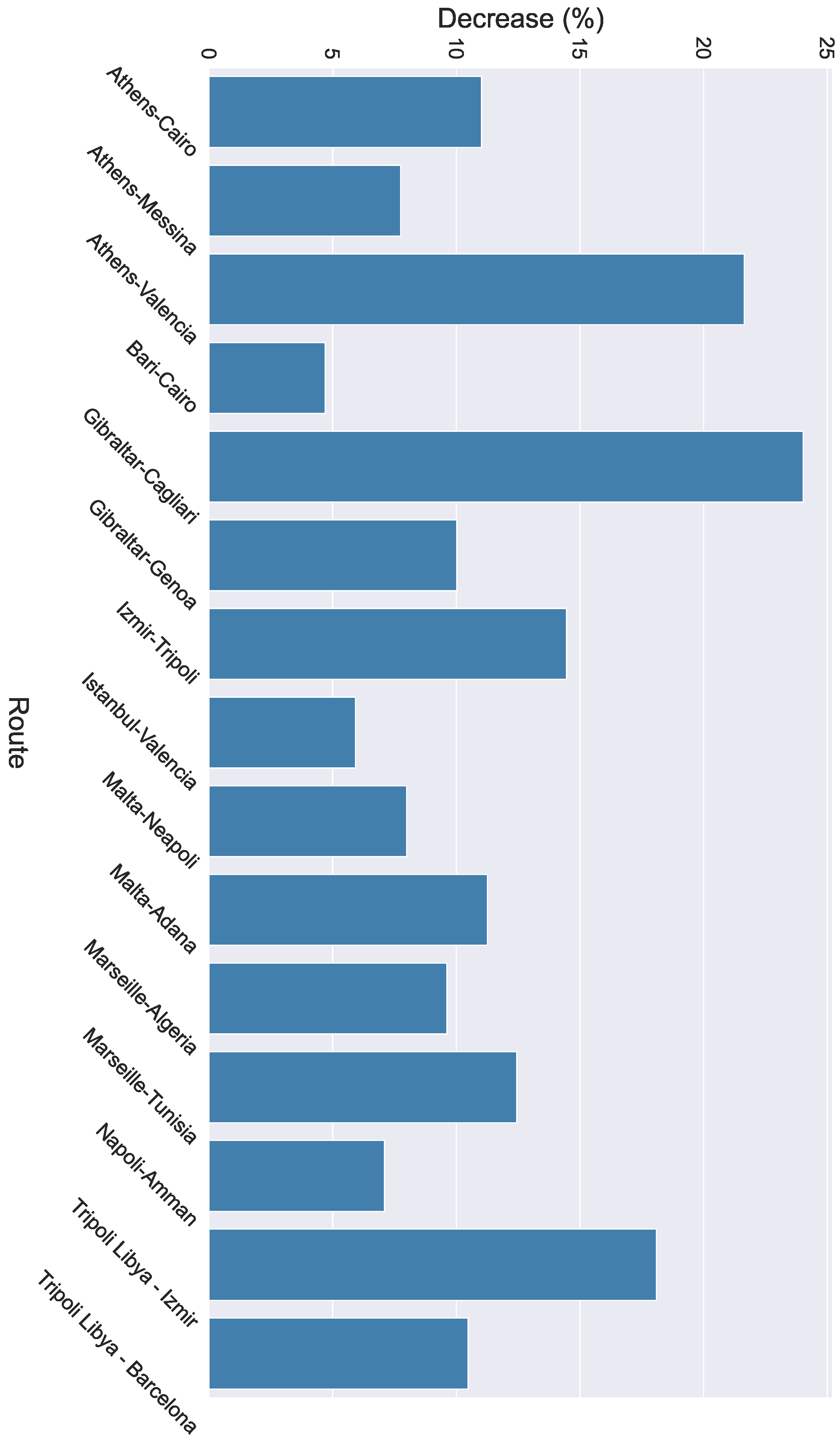
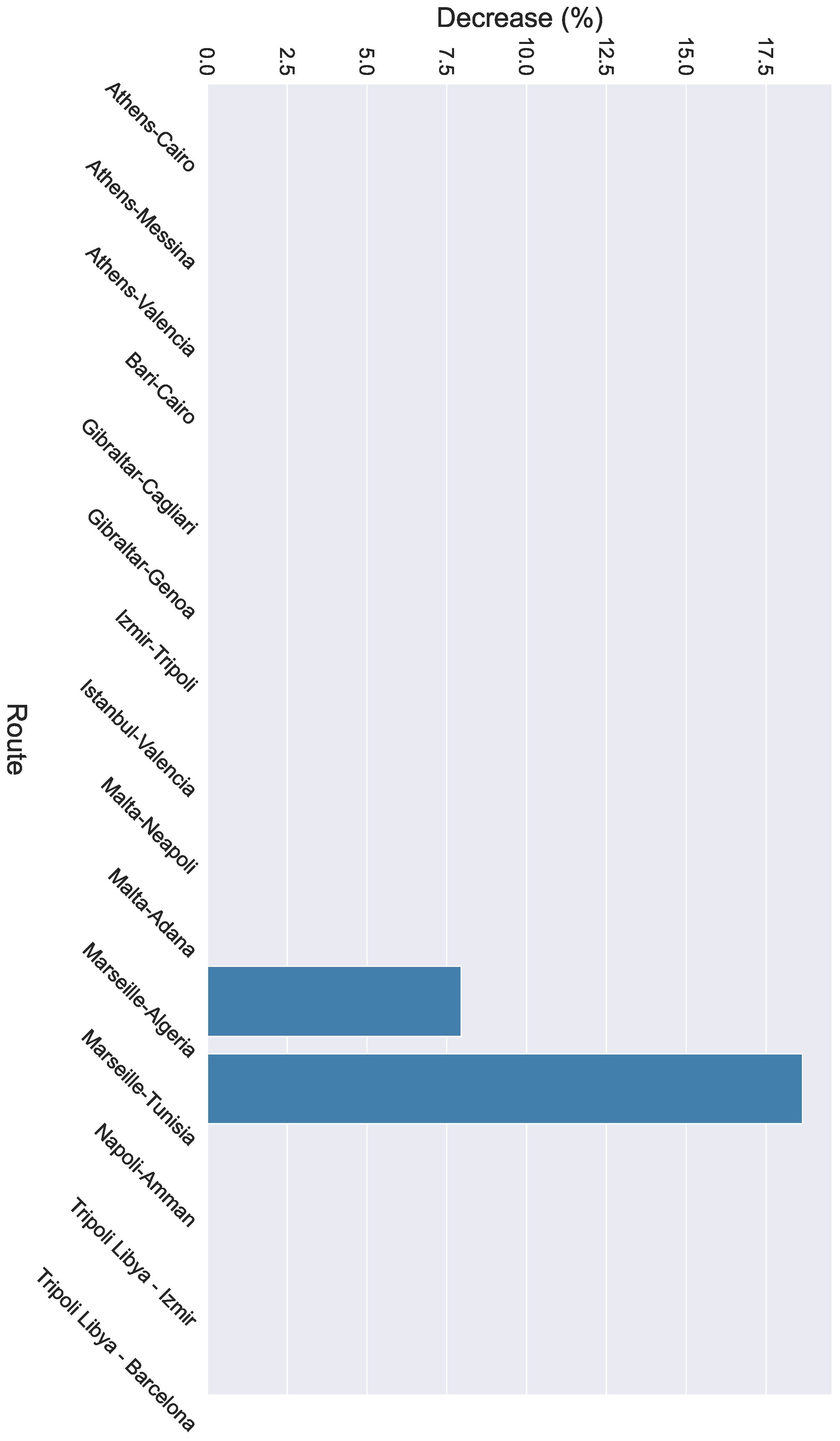
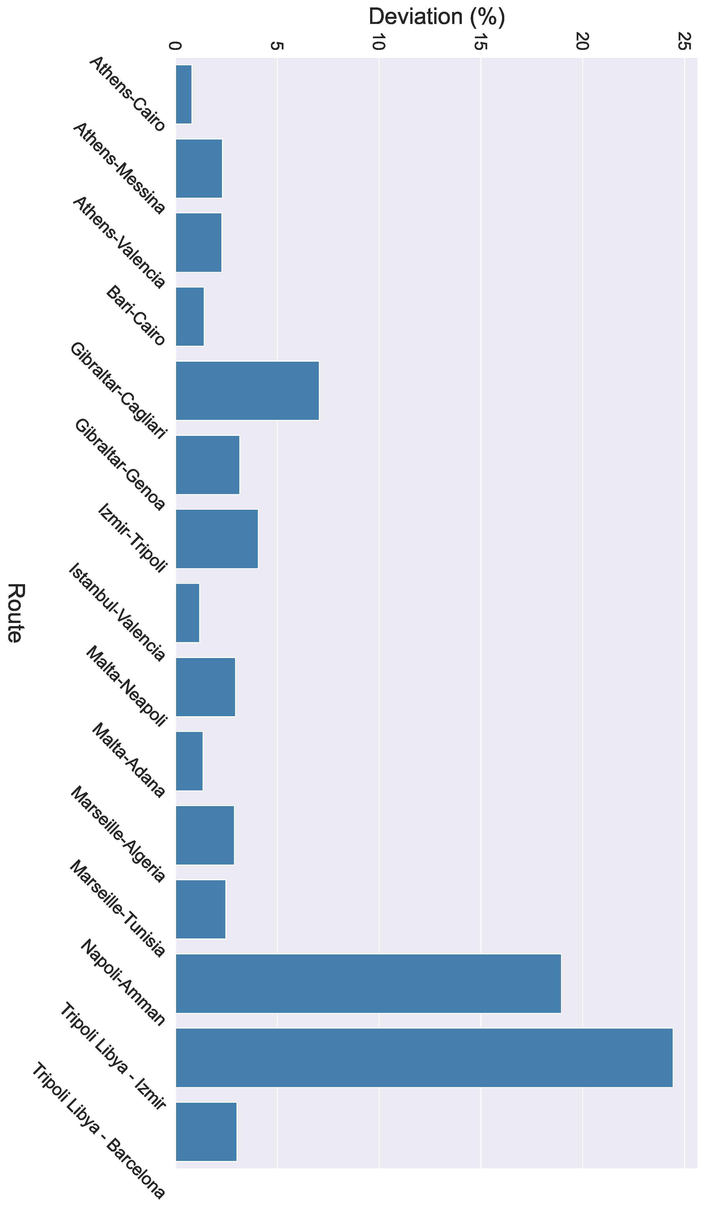
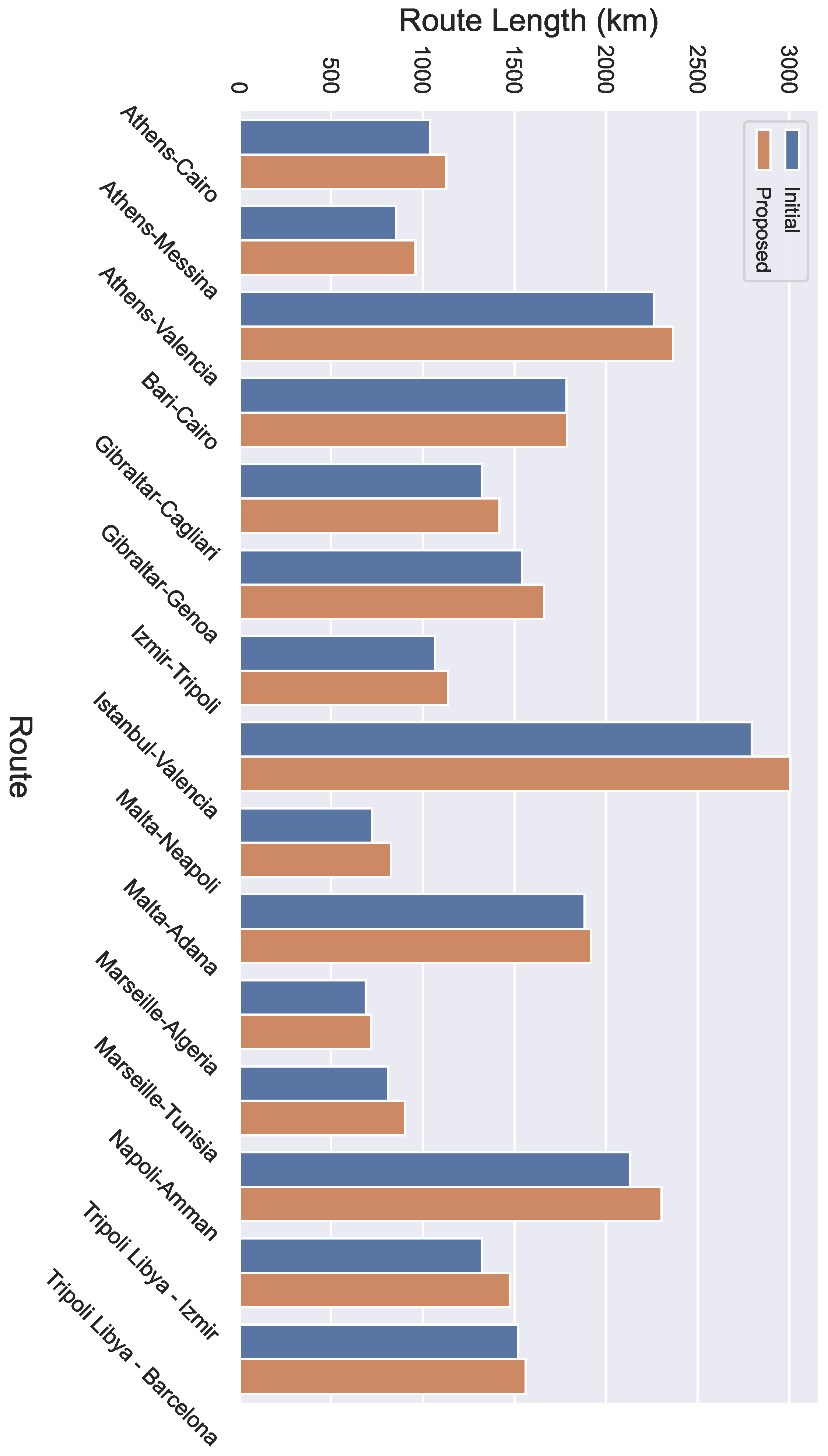
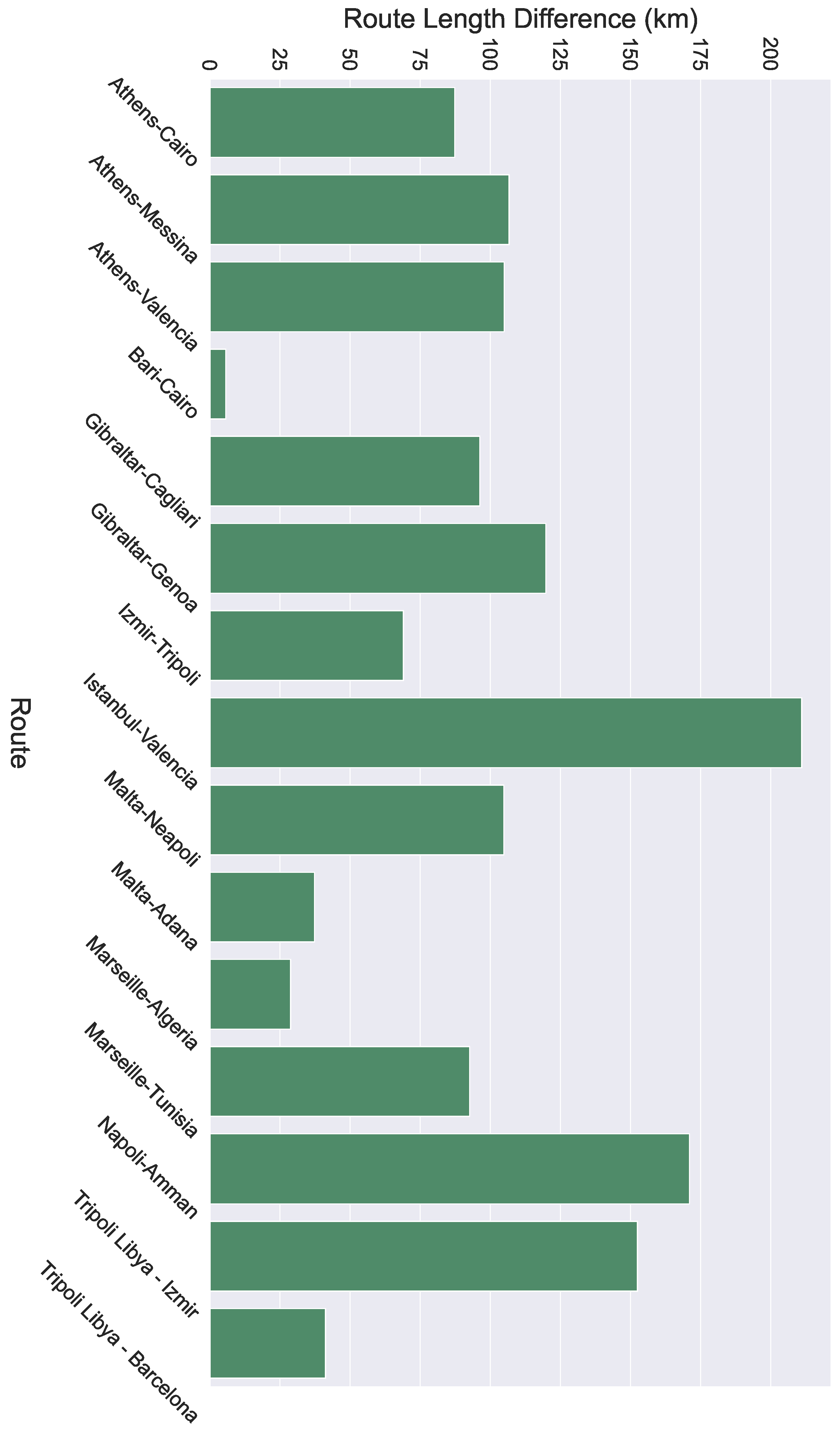
4. Results

To evaluate the proposed weather routing algorithm, we used a dataset that was produced during the study of Kontopoulos et al. [16] and composed of several routes in the Mediterranean sea during the period from January 2022 to March 2022. For evaluation purposes, we chose 15 frequent routes with varying trajectory durations, from one day to several weeks.

The proposed weather routing algorithm takes into account four different weather thresholds. To properly evaluate the algorithm on each threshold, we compared the prevailing weather conditions between the initial routes and the alternate ones. Specifically, for the wave height, we measured its mean value $\overline{h_s^a}$ along the portion (set of centroids) of the route where the adverse conditions were in effect. Then, we measured the mean wave height $\overline{h_s^b}$ of the alternate route during the same period of time. The difference between the mean values to the initial mean value $\overline{h_s^a}$ indicates the percentage of the decrease of the significant wave height $h_s$ (Equation (1)). The percentage-wise decrease of the wave height for each route is demonstrated in Figure 6.

$$H=\frac{\overline{h_s^a}-\overline{h_s^b}}{\overline{h_s^a}}$$

(1)

We can observe that the minimum decrease was $5\%$ in the route from Napoli to Amman and the maximum decrease was approximately $60\%$ in the route from Gibraltar to Cagliari. Furthermore, the mean decrease overall was at about $22\%$. The same process was followed for the other weather thresholds as well. Specifically, for the wave period and the wind speed, we measured their mean values ($\overline{p_s^a}$ and $\overline{v_s^a}$, respectively) along the portion of the route where the adverse conditions were in effect. In the next step, we measured the mean wave period $\overline{p_s^b}$ and the mean wind speed $\overline{v_s^b}$ of the alternate route during the same period of time. The difference between the mean values to the initial mean values indicates the percentage of the decrease of the wave period $p_s$ (Equation (2)) and the wind speed (Equation (3)), respectively. The percentage-wise decrease of the wave period is demonstrated in Figure 7 and the percentage-wise decrease of the wind speed is illustrated in Figure 8 for each route.

$$P=\frac{\overline{p_s^a}-\overline{p_s^b}}{\overline{p_s^a}}$$

(2)

$$V=\frac{\overline{v_s^a}-\overline{v_s^b}}{\overline{v_s^a}}$$

(3)

Regarding the wave period, it is observed that there was a decrease of approximately $11\%$ with a maximum decrease of $24\%$ and a minimum decrease of $4\%$. In terms of wind speed, only the routes of Marseille–Algeria and Napoli–Amman demonstrated a decrease of $8\%$ and $18\%$, respectively. This is due to the fact that in the other routes the wind speed threshold was not exceeded.

Similar to the previous thresholds, the mean direction of the relative difference between the vessel’s heading and the wave’s direction was measured in both routes (initial and alternate). As the denominator, the mean wave direction of the initial route was used and the difference in the wave direction of the routes was used as the numerator. As a result, the percentage-wise deviation of the wave direction between the routes is illustrated in Figure 9. Based on the results, the maximum deviation reached $24\%$ and the minimum deviation was approximately $0.5\%$.

Finally, Figure 10 displays the length of the trajectories for both the initial and the recommended routes, and Figure 11 displays the difference in length between the initial and the recommended routes. It can be observed that the maximum difference in length is approximately 200 km in the case of the Istanbul–Valencia route. Taking into account that the initial route is over 2500 km, a difference of 200 km is only an ≈8% difference, which is an acceptable deviation compared to the cargo loss and potential impact on the regional marine ecology and environment.

5. Conclusions

This paper proposed a weather routing optimization algorithm for cargo loss prevention based on historical AIS data. The proposed algorithm employed historical AIS trajectories to extract the Maritime routes of container ships. IMO guidelines, pertinent literature on the subject, and Maritime expertise from marine engineers and operators were exploited and combined accordingly to outline a consolidated framework, defining the appropriate thresholds of adverse weather conditions for container ships. The evaluation of the algorithm demonstrated a significant decrease in bad weather conditions (e.g., wind speed, wave height) when the (alternative) optimal routes were followed instead of the initial ones.

In future work, we will aim to apply the weighted thresholds for adverse weather conditions. This will eventually result in a more refined, adaptive routing optimization scheme as different weather thresholds (e.g., wind speed and wave direction) will be considered distinctively when planning an alternative route. Therefore, a variety of other factors will be taken into account, such as vessel-specific variables (size, deadweight, displacement, etc.) as well as real-time operational features (speed, power, heading, etc.) acquired from onboard sensor installments.

References

- Zhao, Z.; Ji, K.; Xing, X.; Zou, H.; Zhou, S. Ship surveillance by integration of space-borne SAR and AIS–review of current research. J. Navig. 2014, 67, 177–189. [Google Scholar] [CrossRef]
- Chen, S.; Hong, X.; Khalaf, E.; Morfeq, A.; Alotaibi, N.D. Adaptive B-spline neural network based nonlinear equalization for high-order QAM systems with nonlinear transmit high power amplifier. Digit. Signal Process. 2015, 40, 238–249. [Google Scholar] [CrossRef]
- Zis, T.P.; Psaraftis, H.N.; Ding, L. Ship weather routing: A taxonomy and survey. Ocean. Eng. 2020, 213, 107697. [Google Scholar] [CrossRef]
- Fabbri, T.; Vicen-Bueno, R.; Hunter, A. Multi-criteria weather routing optimization based on ship navigation resistance, risk and travel time. In Proceedings of the 2018 International Conference on Computational Science and Computational Intelligence (CSCI), Las Vegas, NV, USA, 12–14 December 2018; pp. 135–140. [Google Scholar]
- Veneti, A.; Makrygiorgos, A.; Konstantopoulos, C.; Pantziou, G.; Vetsikas, I.A. Minimizing the fuel consumption and the risk in Maritime transportation: A bi-objective weather routing approach. Comput. Oper. Res. 2017, 88, 220–236. [Google Scholar] [CrossRef]
- Yang, J.; Wu, L.; Zheng, J. Multi-Objective Weather Routing Algorithm for Ships: The Perspective of Shipping Company’s Navigation Strategy. J. Mar. Sci. Eng. 2022, 10, 1212. [Google Scholar] [CrossRef]
- Walther, L.; Rizvanolli, A.; Wendebourg, M.; Jahn, C. Modeling and optimization algorithms in ship weather routing. Int. J. -Navig. Marit. Econ. 2016, 4, 31–45. [Google Scholar] [CrossRef]
- Pennino, S.; Gaglione, S.; Innac, A.; Piscopo, V.; Scamardella, A. Development of a new ship adaptive weather routing model based on seakeeping analysis and optimization. J. Mar. Sci. Eng. 2020, 8, 270. [Google Scholar] [CrossRef]
- Shao, W.; Zhou, P.; Thong, S.K. Development of a novel forward dynamic programming method for weather routing. J. Mar. Sci. Technol. 2012, 17, 239–251. [Google Scholar] [CrossRef]
- Wei, S.; Zhou, P. Development of a 3D dynamic programming method for weather routing. Transnav Int. J. Mar. Navig. Saf. Sea Transp. 2012, 6, 79–85. [Google Scholar]
- Papadakis, N.A.; Perakis, A.N. Deterministic minimal time vessel routing. Oper. Res. 1990, 38, 426–438. [Google Scholar] [CrossRef]
- Delitala, A.M.S.; Gallino, S.; Villa, L.a.; Lagouvardos, K.; Drago, A. Weather routing in long-distance Mediterranean routes. Theor. Appl. Climatol. 2010, 102, 125–137. [Google Scholar] [CrossRef]
- Shigunov, V.; Moctar, O.E.; Rathje, H. Operational guidance for prevention of cargo loss and damage on container ships. Ship Technol. Res. 2010, 57, 8–25. [Google Scholar] [CrossRef]
- Maki, A.; Akimoto, Y.; Nagata, Y.; Kobayashi, S.; Kobayashi, E.; Shiotani, S.; Ohsawa, T.; Umeda, N. A new weather-routing system that accounts for ship stability based on a real-coded genetic algorithm. J. Mar. Sci. Technol. 2011, 16, 311–322. [Google Scholar] [CrossRef]
- Perera, L.P.; Soares, C.G. Weather routing and safe ship handling in the future of shipping. Ocean. Eng. 2017, 130, 684–695. [Google Scholar] [CrossRef]
- Kontopoulos, I.; Varlamis, I.; Tserpes, K. A distributed framework for extracting Maritime traffic patterns. Int. J. Geogr. Inf. Sci. 2021, 35, 767–792. [Google Scholar] [CrossRef]
- Murray, B.; Perera, L.P. A dual linear autoencoder approach for vessel trajectory prediction using historical AIS data. Ocean. Eng. 2020, 209, 107478. [Google Scholar] [CrossRef]
- Chen, X.; Liu, Y.; Achuthan, K.; Zhang, X. A ship movement classification based on Automatic Identification System (AIS) data using Convolutional Neural Network. Ocean. Eng. 2020, 218, 108182. [Google Scholar] [CrossRef]
- Volkova, T.A.; Balykina, Y.E.; Bespalov, A. Predicting ship trajectory based on neural networks using AIS data. J. Mar. Sci. Eng. 2021, 9, 254. [Google Scholar] [CrossRef]
- Rong, H.; Teixeira, A.; Soares, C.G. Data mining approach to shipping route characterization and anomaly detection based on AIS data. Ocean. Eng. 2020, 198, 106936. [Google Scholar] [CrossRef]
- Gao, M.; Shi, G.Y. Ship-handling behavior pattern recognition using AIS sub-trajectory clustering analysis based on the T-SNE and spectral clustering algorithms. Ocean. Eng. 2020, 205, 106919. [Google Scholar] [CrossRef]
- Varlamis, I.; Kontopoulos, I.; Tserpes, K.; Etemad, M.; Soares, A.; Matwin, S. Building navigation networks from multi-vessel trajectory data. GeoInformatica 2021, 25, 69–97. [Google Scholar] [CrossRef]
- Kim, S.H.; Roh, M.I.; Oh, M.J.; Park, S.W.; Kim, I.I. Estimation of ship operational efficiency from AIS data using big data technology. Int. J. Nav. Archit. Ocean. Eng. 2020, 12, 440–454. [Google Scholar] [CrossRef]
- Kaklis, D.; Eirinakis, P.; Giannakopoulos, G.; Spyropoulos, C.; Varelas, T.J.; Varlamis, I. A big data approach for Fuel Oil Consumption estimation in the Maritime industry. In Proceedings of the 2022 IEEE Eighth International Conference on Big Data Computing Service and Applications (BigDataService), Newark, CA, USA, 15–18 August 2022; 2022; pp. 39–47. [Google Scholar]
- Kaklis, D.; Giannakopoulos, G.; Varlamis, I.G.; Spyropoulos, C.; Varelas, T.J. A data mining approach for predicting main-engine rotational speed from vessel-data measurements. In Proceedings of the IDEAS’19: Proceedings of the 23rd International Database Applications & Engineering Symposium, Athens, Greece, 10–12 June 2019; ACM: New York, NY, USA, 2019; pp. 1–10. [Google Scholar]
- Kaklis, D.; Giannakopoulos, G.; Varlamis, I.G.; Spyropoulos, C.; Varelas, T.J. Online Training for Fuel Oil Consumption Estimation: A Data Driven Approach. In Proceedings of the 23rd IEEE International Conference on Mobile Data Management (MDM), Paphos, Cyprus, 6–9 June 2022; pp. 1–10. [Google Scholar]