Article

An Intelligent Adequate-Fitting Prediction Method of Coastal Tunnel Rock Deformation Based on the Effective Rank of Hidden Layer

1
School of Civil Engineering, Sun Yat-sen University, Guangzhou 510275, China
2
Guangdong Engineering Research Centre for Major Infrastructure Safety, Guangzhou 510275, China
3
Research Center for Geotechnical Engineering and Information Technology, Sun Yat-sen University, No. 135 Xingang West Road, Guangzhou 510275, China
*
Authors to whom correspondence should be addressed.
J. Mar. Sci. Eng. 2022, 10(11), 1709; https://doi.org/10.3390/jmse10111709
Submission received: 18 October 2022 / Revised: 3 November 2022 / Accepted: 7 November 2022 / Published: 9 November 2022
(This article belongs to the Section Ocean Engineering)

Abstract

:
The intelligent prediction of surrounding rock deformation is of great significance for guiding the design and construction of tunnel projects in coastal areas. The deformation of tunnels in coastal areas is more complex than that of the ground, and the risk of encountering adverse geological conditions is greater. The traditional tunnel deformation prediction method contains the defects of a fixed model, a limited sample number, and it is easy to fall into underfitting and local overfitting. Therefore, the capacity of previous methods is limited by significant error, weak generalization, and poor intelligence. This paper proposes an adequate fitting prediction method for tunnel deformation based on the effective rank theory of the hidden layer nodes’ output matrix to analyze the surrounding rock and predict its deformation intelligently. Based on the traditional BPNN (back propagation neural network) algorithm, the number of hidden layer nodes is determined by the effective rank of the output matrix. Then, the approximation error and degree were adopted to reflect the approximation law of the BPNN to achieve the purpose of overfitting and underfitting control. An optimized BP neural network model for intelligently predicting tunnel deformation is constructed. Then, the optimized BPNN model is applied to a case study of a coastal tunnel in South China. Compared with the prediction method of LR (linear regression) and TS (time series), the results show that the prediction results of the optimized model are in good agreement with the measured values, with strong generalization ability and high intelligence. The proposed method is of guidance to other tunnels surrounding rock deformation prediction and engineering practice.

1. Introduction

The deformation of coastal tunnels has attracted a lot of attention (Zhou, et al. (2020) [1]; Ren, et al. (2021) [2]; Gao, et al. (2021) [3]; Shi, et al. (2021) [4]; Lee, et al. (2020) [5]). During coastal tunnel construction, the surrounding rock is relatively sensitive to excavation, and the large deformation will cause engineering geological disasters such as surface subsidence and cavern collapse. Therefore, the monitoring and intelligent prediction of tunnel rock deformation are significant topics of feedback and control research in underground engineering. In addition, the deformation prediction of the surrounding rock is an important part of the construction, and it is the key to determining reasonable support forms and parameters for ensuring long-term safety. However, the geological conditions of coastal tunnel engineering are complex, and it is difficult to accurately grasp and predict the deformation of the surrounding rock only by the time-consuming and costly on-site measurement. Therefore, it is the key to ensuring the safety of tunnel construction and the stability of the surrounding rock to use an economic and reasonable intelligent prediction method to get the deformation of the coastal tunnel surrounding rock to achieve the purpose of early warning.
There are many methods for predicting and analyzing the deformation of tunnels surrounding rock. Traditional prediction methods such as linear regression predicting, grayscale predicting, support vector machines, time series, and neural network methods are commonly used. Based on (LR) linear regression prediction, scholars mainly use mathematical methods to conduct regression analysis on the measured deformation and obtain the deformation–time relation to predicting the surrounding rock deformation. However, the linear regression prediction model is relatively fixed, and the selection of factors is subjectively dominated. Therefore, the measurement data are discrete, and the prediction accuracy is affected by complex geological conditions (Zhang, et al. (2019) [6]; Fang, et al. (2021) [7]; Luo, et al. (2021) [8]; Zhou, et al. (2018) [9]). In addition, based on grey theory, scholars established a grayscale GM (1,1) model for the deformation prediction through the cumulative summation deformation sequence of a small amount of data. However, the above model is based on data whose changes conform to a certain exponential function, which only suits for short-term prediction (Zhou, et al. (2005) [10]; Xue, et al. (2021) [11]; Huang, et al. (2022) [12]). Simultaneously, based on SVM (support vector machine) and structural risk theory of statistical learning, scholars have built a nonlinear regression function to predict the deformation of tunnel surrounding rock. Since the limitation of the sample number, the accuracy will be affected when the number of samples is too large (Liu, et al. (2017) [13]; Zhang, et al. (2021) [14]; Zhou, et al. (2018) [15]; Zheng, et al. (2022) [16]). In the time series (TS) aspect, scholars also establish the mathematical model relying on deformation statistics to reflect the dynamic dependence contained in the time series when predicting tunnel deformation. However, the model has some limitations (e.g., single linearity, stable monitoring time, equidistant data feature) (Mao, et al. (2011) [17]; Chen (2011) [18]; Shi, et al. (2019) [19]; Shahrour, et al. (2021) [20]; Liu, et al. (2021) [21]). In traditional neural network studies, the common method is building a sample space based on historical surrounding rock deformation data and establishing a neural network model to predict tunnel deformation through learning and training. However, it is difficult to deal with complex geological conditions when approximating the nonlinear function. Otherwise, it is chiefly based on gradient descent, with low learning efficiency, slow convergence speed, and easily falls into a local minimum state (Wu, et al. (2014) [22]; Zhou, et al. (2019) [23]; He, et al. (2020) [24]; Pan, et al. (2021) [25]; Lei, et al. (2021) [26]; Sirimontree, et al. (2022) [27]; Jearsiripongkul, et al. (2022) [28]; Jearsiripongkul, et al. (2022) [29]; Keawsawasvong, et al. (2022) [30]; Ebid, et al. (2021) [31]). The advantages and disadvantages of the various methods mentioned above and their applications are shown in Table 1. To sum up, in the issue of predicting tunnel deformation, previous methods have limitations such as a fixed model, limited by the sample number, prone to underfitting or local overfitting, etc., and the resulting large error, weak generalization ability, and poor intelligence hinder the practical application. Therefore, proposing an optimization model with strong generalization ability, high intelligence, and strong fault tolerance is essential. Then, the various nonlinear deformation problems under complex geological conditions could be dealt with, especially the adequate fitting intelligent prediction of the deformation of the surrounding rock.
According to the abovementioned problems, this paper proposes an intelligent adequate-fitting prediction method based on the effective rank of the hidden layer. On the basis of the traditional BPNN (back propagation neural network) algorithm, the number of hidden layer nodes is determined by the effective rank of the output matrix of the hidden layer nodes. The approximation error and degree were adopted to reflect the approximation law of the BPNN to achieve the purpose of overfitting and underfitting control. Then, an optimized BPNN model for intelligent predicting deformation of tunnel surrounding rock is established. Take a coastal tunnel project as the research object and apply the model to it. The results are consistent with monitored data, which can meet engineering requirements and have practical value.

2. Materials and Methods

2.1. Intelligent Analysis Principle of Tunnel Surrounding Rock Deformation

To analyze the deformation of the surrounding rock, the stress redistribution and the time-dependent deforming in the construction process should be considered, which is nonlinear and highly complex (Das, et al. (2021) [32]; Ye, et al. (2021) [33]; Zhou, et al. (2022) [34]; Han, et al. (2019) [35]), showing complicated mechanical properties. It is difficult to determine the relationship between the actual characteristics of the surrounding rock and its deformation. Considering the surrounding rock deformation is a time-dependent function, different time monitoring points can determine its deformation time series. Therefore, based on in situ monitoring data, it is possible to predict the deformation intelligently which can ensure tunnel construction safety.
To realize an intelligent analysis of the deformation of the surrounding rock, a mathematical model of the deformation time-history curve of the surrounding rock based on the BPNN were established. It can accomplish the prediction and extrapolation of the deformation based on the existing monitoring data.
Considering the monitoring deformation as a time series:
d = d t | d t R ,     t = 1 ,   2 ,    
where d is the deformation of surrounding rock, dt is the monitoring deformation at time t(tn, n is the total deformation data of each monitoring point obtained at the project site).
The time series of deformation data of each monitoring point obtained in situ is taken as the sample space. The prediction output value at time t + 1 is obtained from the monitoring value(1~t). The prediction output value at time t + 2 is obtained from the sequence’s monitoring value from time 2 to t + 1. By analogy, the prediction output value at time n + 1 is obtained from the monitoring value (n − 3~n). From this recursion, the extrapolation and evaluation of the deformation of the surrounding rock are finally completed. The predicted value at time n + 1 is composed of a sequence from n − 2~n + 1, and the value at time n + 2 is extrapolated.
Therefore, the relationship (see Figure 1) between input and output in the intelligent analysis of tunnel surrounding rock deformation (Figure 1) can be defined as:
d t + 1 = F d 1 , d 2 , d 3 , , d t d t + 2 = F d 2 , d 3 , , d t + 1 d t + i = F d i , d i + 1 , , d t + i 1   d ¯ n + 1 = F d n t + 1 , d n t + 2 , d n d ¯ n + 2 = F d n t + 2 , d n t + 3 , d ¯ n + 1 d ¯ n + m = F d n t + m , , d ¯ n + m 1   m t d ¯ n + m = F d ¯ n t + m , , d ¯ n + m 1   m > t
where d t + i is the monitoring deformation at time t + i (i ≥ 1, tn); n is the total deformation data of each monitoring point obtained in situ; d ¯ n + m is the extrapolated deformation of surrounding rock at time n + m (m ≥ 1); F(…) represents the adequate fitting intelligent prediction model.
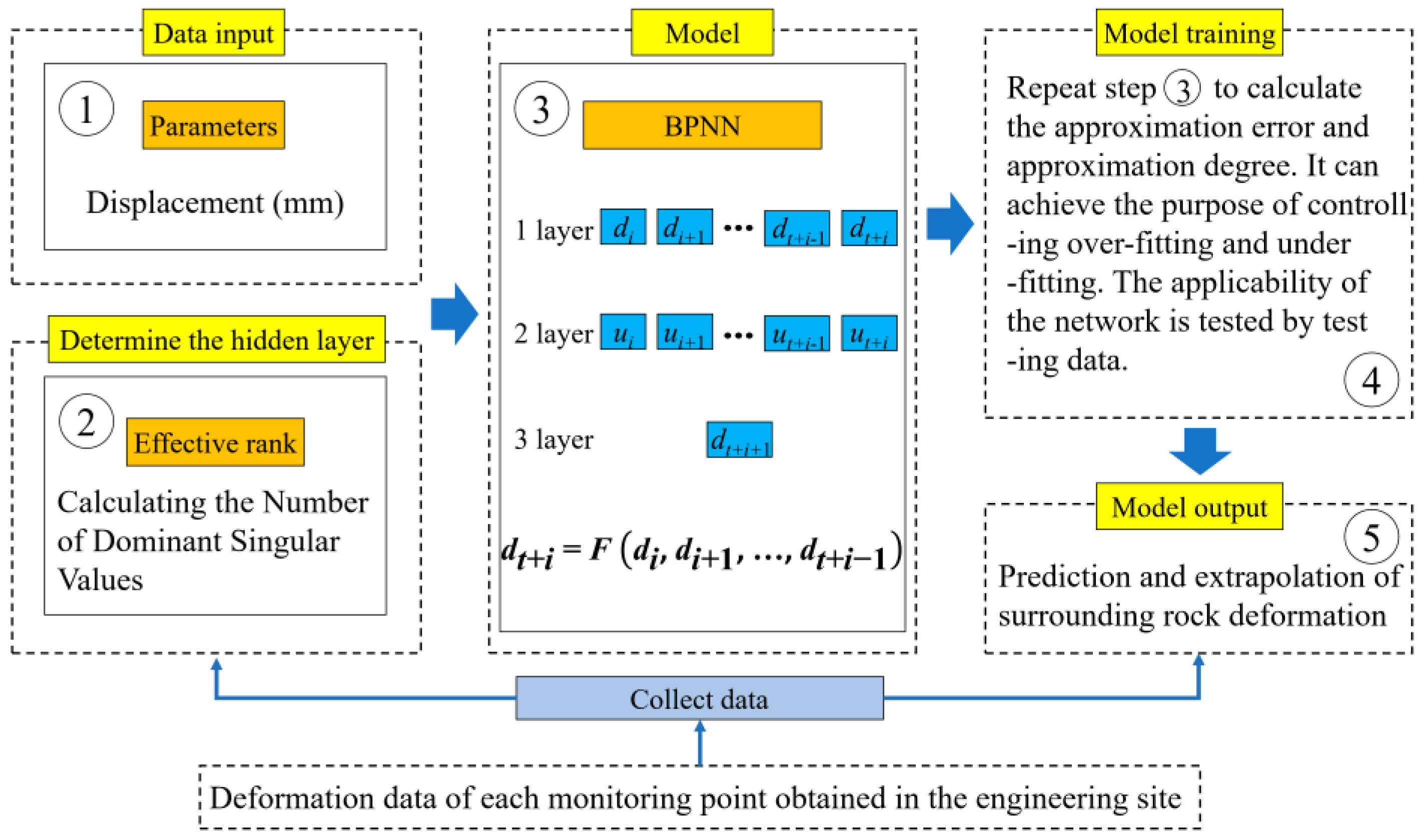
The principle of intelligent analysis of tunnel surrounding rock deformation based on BPNN (see Figure 2) is as follows:
(1) According to the in situ measured deformation data of the surrounding rock, the deformation from 1~t + 1 is regarded as a group, and n − t BPNN training sample spaces are established.
(2) Multiple iterations are performed for each training sample space to make the convergence error reach the set value, and the parameters of the neural network are determined. The number of hidden layer nodes is determined by the effective rank of the hidden layer node of the output matrix.
(3) In the training process, the approximation error and approximation degree are introduced to reflect the approximation regularity of the BPNN, which is used to control overfitting and underfitting, then the optimized BPNN prediction model is established to test samples’ availability.
(4) Calculate the relative error between the measured value and the predicted value of the tunnel surrounding rock deformation.
(5) Finally, the optimized BPNN deformation prediction model is used to extrapolate the time series of the tunnel surrounding rock deformation.

2.2. Intelligent Adequate Fitting Prediction Model of Tunnel Surrounding Rock Deformation Based on Effective Rank of Hidden Layer

2.2.1. Construction of BPNN for Intelligent Prediction of Tunnel Surrounding Rock Deformation

The non-uniformity of the stress distribution and the non-constancy of the deformation rate of the tunnel surrounding rock bring difficulties to the prediction. Therefore, the construction of the BPNN can extrapolate and predict the deformation using the in situ monitored deformation data. The sample space for intelligent prediction of tunnel surrounding rock deformation needs to be established first for establishing the BPNN structure.

2.2.2. Establish Sample Space

During application, a comprehensive evaluation index can better describe the state of the surrounding rock of the tunnel. Actually, it is challenging to collect many indicators and to deal with the resulting complex nonlinear relationship. Therefore, the effects of factors such as excavation-induced material behavior and the role of excavation sequence were ignored in the modeling. Referring to the previous literature (Xie, et al. (2006) [37]; Yao, et al. (2010) [38]), the input number t is set to 4, and the deformation amount of the number t + 1 is regarded as a single sample. Then, apply the 2nd to 6th data as input for the 7th data, and the recursion is finished similarly. When the deformation data are not enough to form a single sample, the prediction deformation value of the previous sample can be used as the input value to extrapolate the tunnel deformation time series.

2.2.3. Construction of BPNN

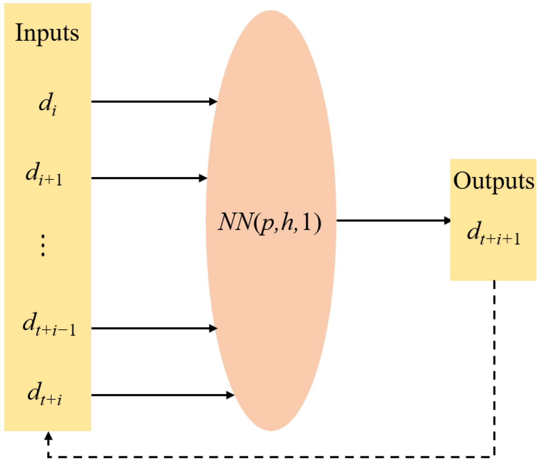
Using a three-layer BPNN NN (p, h, 1) to learn and predict the samples (see Figure 3):
d t + i + 1 = N N p , h , 1 d i , d i + 1 , , d t + i 1 , d t + i
where p is the number of input layer nodes; h is the number of hidden layer nodes; d i , d i + 1 , , d t + i 1 , d t + i are the input node values of the network; d t + i + 1 (1 ≤ i ≤ 20, t = 4) is the output of the network, and n is the total amount of deformation data of each monitoring point acquired in situ. Since it is limited to one-dimensional nonlinear time series, only one node is required. A certain combination operation on 1~t records can derive the value of t + 1.
It is difficult to obtain the monitoring data at the same time interval for the complex in situ environment. Therefore, some deformation monitoring data were organized at equal intervals. In addition, the interpolation method is used to interpolate when there is no monitoring data to ensure that the monitoring data sequence is at equal time intervals (Δt = 1 d). Selecting the input node of the BPNN model as 4, where the deformation value of the next 1d is predicted based on the measured data from 1~4 d.

2.3. Structure Optimization of Tunnel Deformation Prediction Model Based on the Effective Rank of Hidden Layer

As with other layers except for the input layer and output layer, the hidden layer can reduce network error and improve accuracy by increasing the number of hidden layers. However, it also complicates the network, consequently increasing the training time of the network and the tendency of overfitting. Therefore, correctly selecting the number of hidden layer nodes is essential in optimizing (Haykin (2012) [39]; Abadi, et al. (2016) [40]; Lecun, et al. (2015) [41]; Schmidhuber (2015) [42]). At present, there is no effective guidance for selecting the number of hidden layer nodes, which is determined by trial calculation and is difficult to meet practical requirements. Optimizing the structure of the model is based on the effective rank of the hidden layer. Specifically, conduct singular value decomposition on the node of the output matrix of the hidden layer and determine the number of hidden layer nodes according to singular values (Kanjilal, et al. (1995) [43]; Goh, et al. (2008) [44]; Li, et al. (2009) [45]) to finish structure optimization.
The output value of n e t h of the output node is:
n e t h = T l i y i θ l ,   O l = f n e t h
where y i is the output value of the hidden layer node; T l i is the network weight between the hidden and output nodes; θ l is the threshold of the output node l; f x = 1 / 1 + e x .
Assuming that the y i composed matrix is termed A, and T l i composed matrix is called T, then A T = n e t h + θ l = b is given. If the output value of O l of the output node approximates one expected value of a certain sample, then b = n e t h + θ l also approximates a certain value, which constitutes a linear equation system A T = b .
Set the rank of matrix A to r, and then matrix A can conduct singular value decomposition (Hanson and Norris (1981) [46]; Niu et al. (2016) [47]).
The effective rank of matrix A can determine the number of dominant singular values. Ranking the singular values of matrix A as σ 1 σ 2 σ r > 0 , then the normalized ratio is given by:
γ k = [ i = 1 k σ i 2 / i = 1 r σ i 2 ] 1 / 2 ,   0 < k r
Obviously, as k approaches r, γ(k) will approach 1. Given a parameter close to 1, such as β = 0.9999, regarding the smallest value of k that satisfies the γ(k) > β as the effective rank of matrix A (Zhang, et al. (2002) [48]).
In summary, for the neural network model, the hidden layer node output matrix is decomposed by singular value decomposition. The hidden layer nodes that generate small singular values can be considered to be multiple. That is, the appropriate number of nodes in a hidden layer could be determined according to the number of dominant singular values.
In specific practice, first select a BPNN structure and train it to initial convergence. Then, input m learning samples, and calculate the output matrix A i m × n i node of the ith hidden layer (the number of nodes is n i ), and perform singular value decomposition on A i :
A i = U r   0 0 0 V T
Calculating the effective rank k of the matrix A i , it is considered that there are k dominant singular values in r d i a g σ 1 , , σ r . This method is applied to decompose each hidden layer, and finally, a more reasonable intelligent prediction model structure can be obtained.

2.4. BPNN Adequate Fitting for Intelligent Prediction of Tunnel Surrounding Rock Deformation

According to the optimization based on the effective rank of the hidden layer, carry out adequate fitting optimization analysis. The practical application indicates that: in the training process, the prediction error is large when the sample size is too small. As the sample increases, the fitting error decreases, and the initial prediction error also decreases, but when the fitting error decreases to a certain value, the prediction error increases inversely, indicating that the generalization ability decreases. This is the phenomenon of underfitting, and local overfitting encountered in the BPNN modeling process (Wang, et al. (2022) [49]). Considering the abovementioned problems, the approximation error and degree (Tin-Yau, et al. (1996) [50]; Himmelblau (2008) [51]) were introduced to reflect the approximation regularity of BPNN and to control the underfitting and overfitting.
The known samples are divided into training samples and monitoring samples, the latter does not participate in training but participates in monitoring training. Input the training samples into the BPNN model for training. When the training reaches a certain level, using the weights and thresholds to predict the monitoring samples to obtain the prediction error. Combining the training and prediction errors of the monitoring samples, the following definitions are defined:
(1) Approximation error:
e n = n 1 / n e 1 + n c / n e c
where e n is the approximation error; e 1 is the absolute average relative error of the monitoring samples; e c is absolute average relative error of the prediction value; n 1 is the number of training samples; n c is the number of monitoring samples; n is the number of known samples; n 1 / n and n c / n are the weights of training and monitoring samples to the approximation error, respectively.
(2) Approximation degree:
d n = 100 / e x p 10 e n
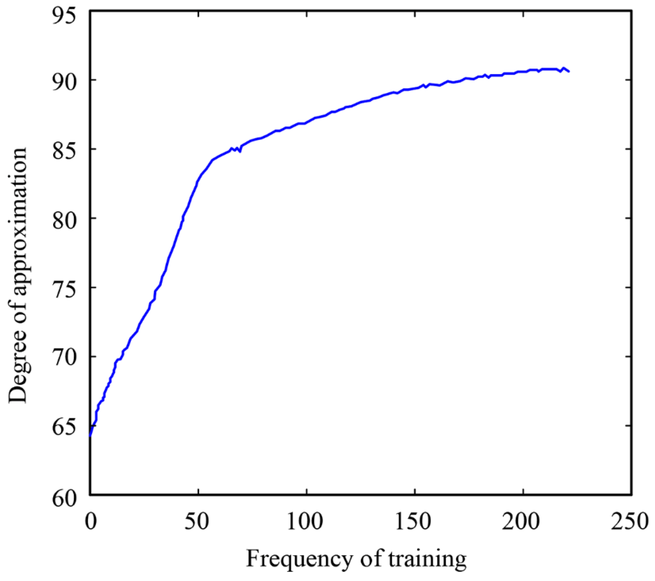
Obviously, a smaller approximation error e n will bring a larger approximation degree d n , resulting in better predictability. When the approximation error e n is close to 0, the approximation degree d n is close to 100. Since the prediction error of the monitoring samples is added, only when the prediction error is controlled within a small range, the approximation error will decrease with the reduction of the average relative error of the training samples. Therefore, the approximation degree d n increases first and then decreases with the increase in training times, which means that the prediction error of the monitoring sample decreases first and then increases. Additionally, the prediction ability of the network model declines (overfitting occurs). Therefore, the approximation d n could be used to control overfitting during training.
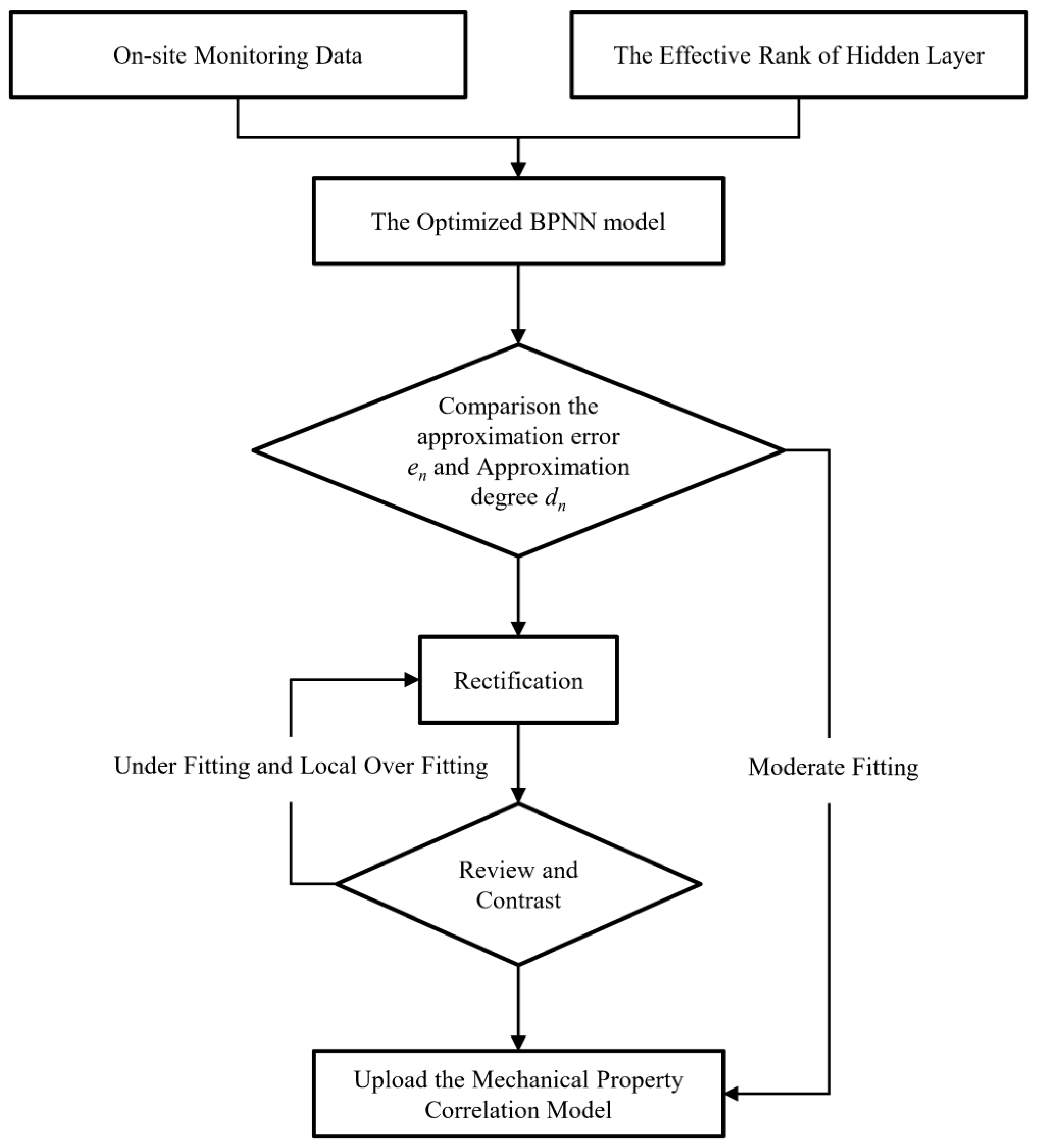
The specific applying process:
➀ Input the training samples into the BPNN model for intelligent prediction of tunnel surrounding rock deformation and specify iteration times.
➁ Stop training iterates to the specified times, and the monitoring samples with the weights and thresholds can be predicted. The approximation error e n and approximation degree d n are calculated according to Equations (7) and (8).
➂ Carry out the next stage of training and repeat step 2.
➃ When the error of the training sample meets the requirement, stop training; otherwise, return to step 3.
➄ Observing d n : If the approximation degree keeps increasing (without overfitting) during the training, the final weights and thresholds should be used for actual prediction. If the approximation degree increases first and decreases subsequently (overfitting appears), the weight and threshold of the maximum approximation degree should be adopted for actual prediction.
The research methodology and process of this paper are shown in Figure 4.

3. Results and Discussion

3.1. Case Study

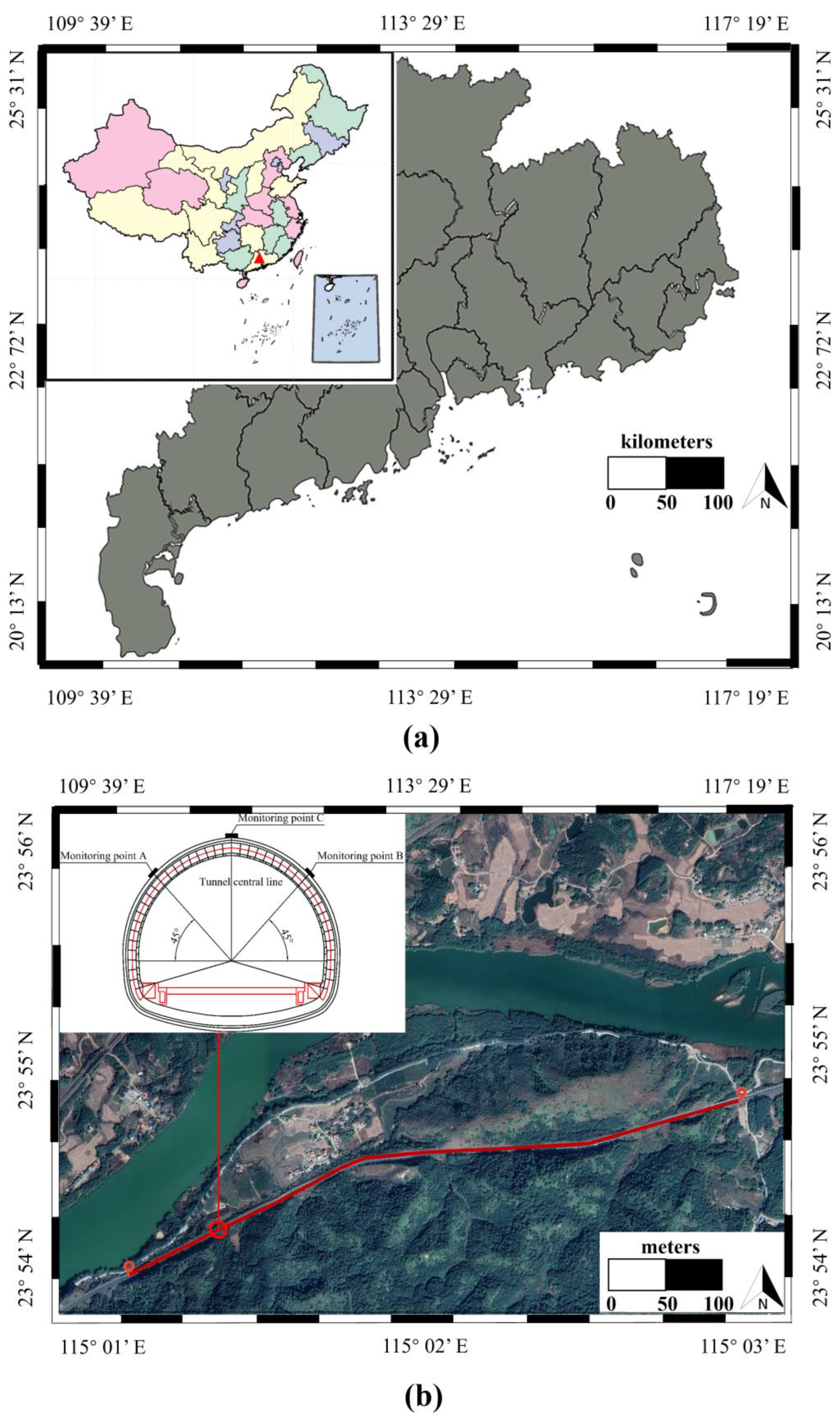
In order to verify the proposed prediction model, this paper adapts a coastal tunnel project in South China (Figure 5a). The terrain along the tunnel fluctuates greatly, and the lithological boundary of the stratum changes complicatedly. Selecting a representative dangerous section, which is uniformly distributed throughout the tunnel, to acquire the data on the tunnel surrounding rock deformation. The tunnel is a non-pressure, concrete-lined water supply tunnel with a circular arch straight wall section. The width of the tunnel is 10.5 m, and the height is 5.0 m. The support is designed according to the New Austrian method, where shotcrete and bolts are the primary support. The surrounding rocks at both ends of the tunnel are classified mainly as I and II. The middle part is transitioned to III and IV, and the geological conditions are poor. Therefore, after the completion of tunnel excavation and initial support, the measuring points are buried at the elevation of the inner rail top surface of the vault and the sidewall to measure the vault subsidence and horizontal convergence (Figure 5b). The representative section is Class III surrounding rock. In general, the measurement frequency is once a day first and then reduces according to the deformation, and the measurement points are arranged in a group every 5 m. Due to this, the deformation rate at the beginning of the experiments is obviously more than the one in the later experiments.

3.2. Collected Database

An extensive field monitoring database of 84 was used in this study. Select some of the surrounding rock deformation monitoring data (20 July–11 August) obtained from three measuring points A, B, and C in representative sections to establish 20 training samples, respectively. Some of the latter data are used for the validation of the extrapolation accuracy of the model (12–16 August). The first four data sets of the surrounding rock deformation are picked as the input data, and then the fifth data set is predicted. By analogy, 20 model training samples are established. Finally, adding the predicted value of the last step to the original training sample to form the 21st training sample. Then, the extrapolated deformation value of the next time step is predicted. By analogy, five extrapolated values are calculated.

3.3. The Establishment and Normalization of Intelligent Prediction Model Samples

Take measurement point A as an illustration. The training process is based on the abovementioned 20 samples. By selecting four monitoring samples, the approximation error and degree could be calculated to reflect the approximation regularity of the BPNN, which is used to control underfitting and overfitting. The prediction ability can also be tested by calculating the prediction error.
To reduce the learning time, the input and output data are normalized, where the transformation is between [0.1~0.9]:
x i = 0.1 + 0.8 x i x m i n x m a x x m i n
where x i is the i-th original data; x m i n and x m a x are the minimum and maximum values in the original data, respectively, and the normalized x i is between 0 and 1.

3.4. Adequate Fit Training for Intelligent Prediction Models

The nodes of the hidden layer should not exceed the training samples. Therefore, firstly select the network structure with 20 nodes in the hidden layer. After the initial convergence, the calculated effective rank is 3. Then, the number of nodes in the hidden layer is set to 20, 10, 5, 4, and 3, respectively, and the resulting effective ranks are all 3. Therefore, the BPNN structure of the deformation prediction model of measuring point A is 4-3-1.
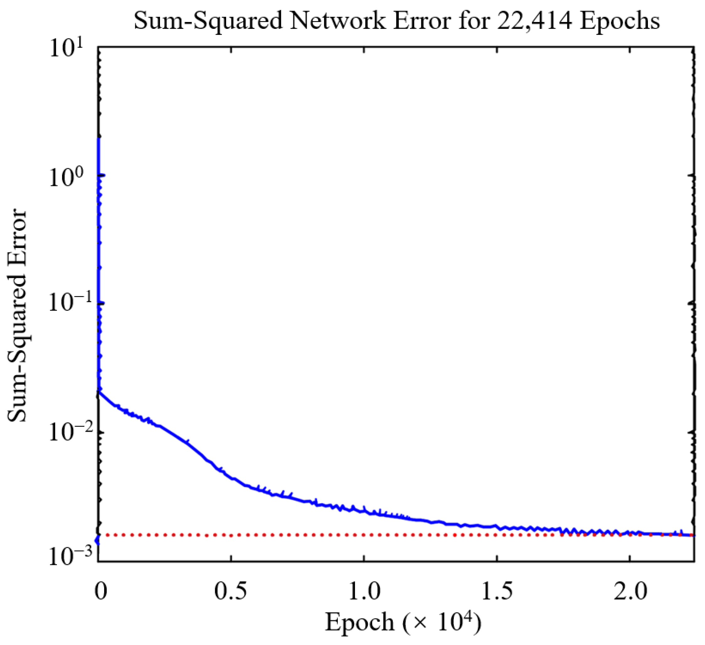
Re-inputting the 20 training samples and 4 monitoring samples into the optimized BPNN deformation prediction model for learning, and the adequate fitting of the network model is achieved through controlling approximation error and degree. The training error curve is shown in Figure 6, and the approximation curve is shown in Figure 7. Add the predicted value of the last time step to the original training sample. Similarly, re-input the 21 training samples and 4 monitoring samples into the model and predict the next step’s extrapolated deformation. Then, the extrapolated deformation value is added to the learning as a new sample, and the next extrapolated value is calculated.

3.5. Verification Analysis

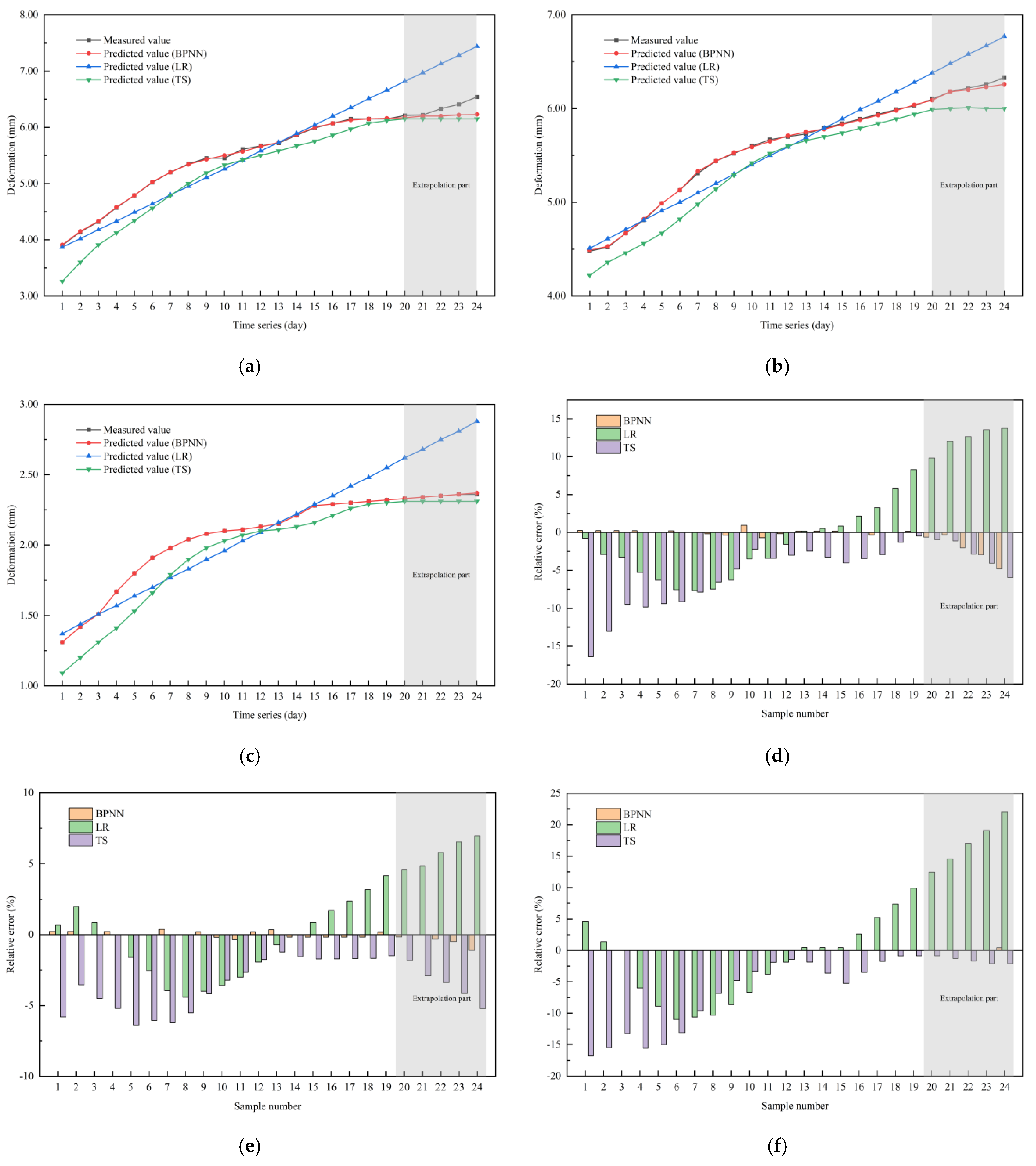
To further analyze the characteristics of the intelligent prediction for the tunnel surrounding rock deformation, we take part of the prediction and extrapolation results of measurement points A, B, and C as a presentation, and compare them with monitoring data. Here, to evaluate the performance of the proposed model, conventional LR and TS methods were also introduced in this paper. One of the LR models uses the one-variable linear regression method. The TS model, on the other hand, uses a one-time moving average method. The relationship between observations and predictions for three models is also illustrated in Figure 8a–c). Then, the error between the prediction results of the BPNN model, LR model, TS model, and the monitoring data is obtained (Figure 8d–f). From the comparison of prediction results, the three models demonstrate different accuracies according to different trends of monitoring data. The LR model has high prediction accuracy when the monitoring data itself is relatively linear (Figure 8b). However, when the monitoring data are non-linear, the comparison between the predicted and the measured value of the surrounding rock deformation indicates poor agreement (Figure 8a,c)). The TS model simulates the trend better, but with larger errors. On the contrary, the prediction results of the BPNN model show good accuracy no matter in the case of linear or nonlinear data. It shows its universality is better than the LR model and TS model.
From Figure 8d–f, one can find that the linear regression model has a small error in the middle of the time series (maximum relative error 3.39%). Further, the TS model has smaller and smaller errors over time (the minimum error can reach 0.49%). On the whole, it is obvious that the errors from BPNN models generally are smaller than that of LR and TS. This can be explained by the intelligent adequate fitting prediction method, which uses the approximation error and degree to minimize the generalization and training error. While the LR may tend to fall into a local optimal solution, the TS models, however, require error adjustment through a large amount of historical data.
Moreover, looking at the extrapolated data from the different models, it can be noted that all three have certain limitations. The poor prediction of extrapolated data by LR models is a natural consequence of the complex ground stress redistribution. For the TS model, the prediction of the extrapolated data is more accurate. Overall, the predictions of the neural network model are better, except for the case when the extrapolated data have large abrupt changes.
Referring to previous studies (Ebid, et al. (2022) [52]; Deifalla, et al. (2022) [53]), the coefficient of determination (R2), root mean square error (RMSE) and mean square error (MAE) can be compared for each model at points A, B and C, respectively (Table 2).
R2, RMSE and MAE were used to evaluate the accuracy of the three selected models. The LR model after one-dimensional linear regression method had the worst performance (R2 = 0.88~0.94, RMSE = 0.46~0.94, MAE = 0.11~0.22).
The most accurate model was the improved BPNN. It demonstrated outstanding performance using R2, RMSE, and MAE with values of 0.99, 0.06, and 0.01, respectively. However, its extrapolation accuracy needs further improvement.
The TS model makes full use of the historical data and exhibits better extrapolation prediction accuracy. Further optimization of the BPNN combined with the TS model can be considered in the follow-up study.
To sum up, it is feasible to solve the deformation prediction of tunnel surrounding rock with our model.

4. Conclusions

(1) On the basis of the traditional BPNN algorithm, this paper proposes an intelligent adequate fitting prediction method of tunnel deformation based on the effective rank of the hidden layer node of the output matrix to predict the deformation, which improves the prediction accuracy and solves the problem of poor generalization and intelligence.
(2) In this paper, the number of hidden layer nodes is determined by the effective rank of the output matrix of the hidden layer nodes. The approximation error and degree are adopted to reflect the approximation degree to control overfitting and underfitting. Based on adequate fitting, intelligently predicting the deformation of the surrounding rock of the tunnel is achieved (R2 = 0.99~1.00, RMSE = 0.01~0.06, MAE = 0.01), which provides an effective new method for the prediction of the deformation of the tunnel.
(3) The optimized BPNN model constructed in this paper has successfully predicted the surrounding rock deformation of a coastal tunnel in South China. This model can better meet the engineering requirement, which can guide significance for deformation prediction and stability analysis of similar tunnels.

Author Contributions

Conceptualization, J.L., Z.L. and C.Z.; methodology, J.L. and Z.L.; software, J.L. and Y.W.; validation, J.L., C.X. and Y.W.; formal analysis, J.L.; investigation, J.L., Z.L. and C.Z.; resources, Z.L. and C.Z.; data curation, J.L., C.X. and Y.W.; writing—original draft preparation, J.L., Z.L. and C.Z.; writing—review and editing, J.L., Z.L. and C.Z.; visualization, J.L.; supervision, Z.L.; project administration, Z.L. and C.Z.; funding acquisition, Z.L. and C.Z. All authors have read and agreed to the published version of the manuscript.

Funding

The work presented in this article was supported by the National Natural Science Foundation of China (NSFC) (Grant No.41977230), the Special Fund Key Project of Applied Science and Technology Research and Development in Guangdong (Grant No. 2015B090925016, No. 2016B010124007).

Institutional Review Board Statement

Not applicable.

Informed Consent Statement

Not applicable.

Data Availability Statement

Not applicable.

Conflicts of Interest

The authors declare that they have no known competing financial interests or personal relationships that could have appeared to influence the work reported in this paper.

References

  1. Zhou, C.; Li, A.; Liu, Z. Study on the Influence of Parallel Fold Structure on Deformation of Tunnel Surrounding Rocks. Mod. Tunn. Technol. 2020, 57, 65. [Google Scholar]
  2. Ren, Q.; Xu, L.; Zhu, A.; Shan, M.; Zhang, L.; Gu, J.; Shen, L. Comprehensive safety evaluation method of surrounding rock during underground cavern construction. Undergr. Space 2021, 6, 46–61. [Google Scholar] [CrossRef]
  3. Gao, B.Y.; Wang, R.R.; Lin, C.J.; Guo, X.; Liu, B.; Zhang, W.G. TBM penetration rate prediction based on the long short-term memory neural network. Undergr. Space 2021, 6, 718–731. [Google Scholar] [CrossRef]
  4. Shi, Y.; Gao, F.; Wang, N.; Yin, Z. Coupled flow-seepage-elastoplastic modeling for competition mechanism between lateral instability and tunnel erosion of a submarine pipeline. J. Mar. Sci. Eng. Sci. 2021, 9, 889. [Google Scholar] [CrossRef]
  5. Lee, S.; Lee, S.; Kwon, S.-D. Effects of Topside Structures and Wind Profile on Wind Tunnel Testing of FPSO Vessel Models. J. Mar. Sci. Eng. Sci. 2020, 8, 422. [Google Scholar] [CrossRef]
  6. Zhang, W.; Dai, B.B.; Liu, Z.; Zhou, C.Y. On the non-Darcian seepage flow field around a deeply buried tunnel after excavation. Bull. Eng. Geol. Environ. 2019, 78, 311–323. [Google Scholar] [CrossRef]
  7. Fang, Z.; Yang, W.; Wang, J.; Shi, J.; Ba, X.; Wang, H. Study on the minimum safe thickness of water-proof rock mass in front of deep-buried tunnels. J. Cent. South Univ. Sci. Technol. 2021, 52, 2805–2816. [Google Scholar]
  8. Luo, Y.; Huang, J.H.; Lu, W.B.; Zhang, G.; Li, X.P.; Song, K.W. Study on transient unloading loosening simulation test of excavation of jointed rock mass. Proc. Inst. Civ. Eng. -Geotech. Eng. 2021, 174, 645–656. [Google Scholar] [CrossRef]
  9. Zhou, X.P.; Huang, X.C.; Liu, P.F.; Li, T.F. A probabilistic method to analyze collapse failure of shallow rectangular tunnels. Tunn. Undergr. Space Technol. 2018, 82, 9–19. [Google Scholar] [CrossRef]
  10. Zhou, C.; Zhang, L.; Huang, X. Classification of Rocks Surrounding Tunnel Based on Improved BP Network Algorithm. Earth Sci. 2005, 30, 480–486. [Google Scholar]
  11. Xue, Y.; Ma, X.; Qiu, D.; Yang, W.; Li, X.; Kong, F.; Zhou, B.; Qu, C. Analysis of the factors influencing the nonuniform deformation and a deformation prediction model of soft rock tunnels by data mining. Tunn. Undergr. Space Technol. 2021, 109, 103769. [Google Scholar] [CrossRef]
  12. Xue, Y.; Ma, X.; Qiu, D.; Yang, W.; Li, X.; Kong, F.; Zhou, B.; Qu, C. A Gray Wolf Optimization-Based Improved Probabilistic Neural Network Algorithm for Surrounding Rock Squeezing Classification in Tunnel Engineering. Front. Earth Sci. 2022, 10, 857463. [Google Scholar]
  13. Liu, K.Y.; Liu, B.G. Optimization of smooth blasting parameters for mountain tunnel construction with specified control indices based on a GA and ISVR coupling algorithm. Tunn. Undergr. Space Technol. 2017, 70, 363–374. [Google Scholar] [CrossRef]
  14. Zhang, W.G.; Li, H.R.; Wu, C.Z.; Li, Y.Q.; Liu, Z.Q.; Liu, H.L. Soft computing approach for prediction of surface settlement induced by earth pressure balance shield tunneling. Undergr. Space 2021, 6, 353–363. [Google Scholar] [CrossRef]
  15. Zhou, X.P.; Huang, X.C.; Li, J.X. Reliability Assessment of Tunnel Based on P-Wave Seismic Velocity. Int. J. Geomech. 2018, 18, 06018030. [Google Scholar] [CrossRef]
  16. Zheng, Y.; Lv, X.; Qian, L.; Liu, X. An Optimal BP Neural Network Track Prediction Method Based on a GA–ACO Hybrid Algorithm. J. Mar. Sci. Eng. Sci. 2022, 10, 1399. [Google Scholar] [CrossRef]
  17. Mao, G.X.; Xia, Y.Y.; Liu, L.W. Time Series Forecasting of Tunnel Surrounding Rock Displacement. In Proceedings of the International Conference on Civil Engineering and Building Materials (CEBM), Kunming, China, 26–28 July 2011; Volume 261–263, pp. 1789–1793. [Google Scholar]
  18. Chen, L. Macro-grammatical evolution for nonlinear time series modeling-a case study of reservoir inflow forecasting. Eng. Comput. 2011, 27, 393–404. [Google Scholar] [CrossRef]
  19. Shi, S.; Zhao, R.; Li, S.; Xie, X.; Li, L.; Zhou, Z.; Liu, H. Intelligent prediction of surrounding rock deformation of shallow buried highway tunnel and its engineering application. Tunn. Undergr. Space Technol. 2019, 90, 1–11. [Google Scholar] [CrossRef]
  20. Shahrour, I.; Zhang, W.G. Use of soft computing techniques for tunneling optimization of tunnel boring machines. Undergr. Space 2021, 6, 233–239. [Google Scholar] [CrossRef]
  21. Liu, Z.; Ming, W.H.; Li, J.M.; Zhou, C.Y.; Zhang, L.H. Numerical prediction of the optimal shield tunneling strategy for tunnel construction in karst regions. PLoS ONE 2021, 16, e0252733. [Google Scholar] [CrossRef]
  22. Wu, Q.D.; Yan, B.; Zhang, C.; Wang, L.; Ning, G.B.; Yu, B. Displacement Prediction of Tunnel Surrounding Rock: A Comparison of Support Vector Machine and Artificial Neural Network. Math. Probl. Eng. 2014, 2014, 351496. [Google Scholar] [CrossRef]
  23. Zhou, C.Y.; Ouyang, J.W.; Ming, W.H.; Zhang, G.H.; Du, Z.C.; Liu, Z. A Stratigraphic Prediction Method Based on Machine Learning. Appl. Sci. 2019, 9, 3553. [Google Scholar] [CrossRef] [Green Version]
  24. He, P.; Xu, F.; Sun, S.Q. Nonlinear deformation prediction of tunnel surrounding rock with computational intelligence approaches. Geomat. Nat. Hazards Risk 2020, 11, 414–427. [Google Scholar] [CrossRef] [Green Version]
  25. Pan, Y.; Chen, L.; Wang, J.; Ma, H.; Cai, S.; Pu, S.; Duan, J.; Gao, L.; Li, E. Research on deformation prediction of tunnel surrounding rock using the model combining firefly algorithm and nonlinear auto-regressive dynamic neural network. Eng. Comput. 2021, 37, 1443–1453. [Google Scholar] [CrossRef]
  26. Lei, X.; Ouyang, J.; Wang, Y.; Wang, X.; Zhang, X.; Chen, F.; Xia, C.; Liu, Z.; Zhou, C. Thermal-Mechanical Coupling Evaluation of the Panel Performance of a Prefabricated Cabin-Type Substation Based on Machine Learning. Fire 2021, 4, 93. [Google Scholar] [CrossRef]
  27. Sirimontree, S.; Keawsawasvong, S.; Ngamkhanong, C.; Seehavong, S.; Sangjinda, K.; Jearsiripongkul, T.; Thongchom, C.; Nuaklong, P. Neural Network-Based Prediction Model for the Stability of Unlined Elliptical Tunnels in Cohesive-Frictional Soils. Buildings 2022, 12, 444. [Google Scholar] [CrossRef]
  28. Jearsiripongkul, T.; Keawsawasvong, S.; Banyong, R.; Seehavong, S.; Sangjinda, K.; Thongchom, C.; Chavda, J.T.; Ngamkhanong, C. Stability Evaluations of Unlined Horseshoe Tunnels Based on Extreme Learning Neural Network. Computation 2022, 10, 81. [Google Scholar] [CrossRef]
  29. Jearsiripongkul, T.; Keawsawasvong, S.; Thongchom, C.; Ngamkhanong, C. Prediction of the Stability of Various Tunnel Shapes Based on Hoek–Brown Failure Criterion Using Artificial Neural Network (ANN). Sustainability 2022, 14, 4533. [Google Scholar] [CrossRef]
  30. Keawsawasvong, S.; Seehavong, S.; Ngamkhanong, C. Application of Artificial Neural Networks for Predicting the Stability of Rectangular Tunnels in Hoek-Brown Rock Masses. Front. Built Environ. 2022, 8, 837745. [Google Scholar] [CrossRef]
  31. Ebid, A.M.; Deifalla, A. Prediction of shear strength of FRP reinforced beams with and without stirrups using (GP) technique. Ain Shams Eng. J. 2021, 12, 2493–2510. [Google Scholar] [CrossRef]
  32. Das, R.; Singh, T.N. Effect of rock bolt support mechanism on tunnel deformation in jointed rockmass: A numerical approach. Undergr. Space 2021, 6, 409–420. [Google Scholar] [CrossRef]
  33. Ye, S.H.; Zhao, Z.F.; Wang, D.Q. Deformation analysis and safety assessment of existing metro tunnels affected by excavation of a foundation pit. Undergr. Space 2021, 6, 421–431. [Google Scholar] [CrossRef]
  34. Zhou, Z.; Zhang, J.J.; Gong, C.J. Automatic detection method of tunnel lining multi-defects via an enhanced You Only Look Once network. Comput. -Aided Civ. Infrastruct. Eng. 2022, 37, 762–780. [Google Scholar] [CrossRef]
  35. Han, S.; Jeng, D.-S.; Tsai, C.-C. Response of a porous seabed around an immersed tunnel under wave loading: Meshfree model. J. Mar. Sci. Eng. Sci. 2019, 7, 369. [Google Scholar] [CrossRef]
  36. Zeng, Q.; Liao, J.; Huang, X.; Ming, W.; Gao, Y.; Zhou, C.; Liu, Z. An Intelligent Correlation Real-Time Analysis Method for the Mechanical Properties of Members in Super-Span Valve Hall Grid Structure Hoisting Process. Sensors 2022, 22, 8111. [Google Scholar] [CrossRef]
  37. Xie, J.X.; Cheng, C.T.; Chau, K.W.; Pei, Y.Z. A hybrid adaptive time-delay neural network model for multi-step-ahead prediction of sunspot activity. Int. J. Environ. Pollut. 2006, 28, 364–381. [Google Scholar] [CrossRef] [Green Version]
  38. Yao, B.Z.; Yang, C.Y.; Yao, J.B.; Sun, J.A. Tunnel Surrounding Rock Displacement Prediction Using Support Vector Machine. Int. J. Comput. Intell. Syst. 2010, 3, 843–852. [Google Scholar]
  39. Haykin, S. Neural Networks: A Guided Tour Nonlinear Biomedical Signal Processing: Fuzzy Logic, Neural Networks, and New Algorithms; Wiley-IEEE Press: Hoboken, NJ, USA, 2012; Volume 1, pp. 53–68. [Google Scholar]
  40. Abadi, M.; Chu, A.; Goodfellow, I.; McMahan, H.B.; Mironov, I.; Talwar, K.; Zhang, L. Deep learning with differential privacy. In Proceedings of the ACM Conference on Computer and Communications Security, Vienna, Austria, 24–28 October 2016; pp. 308–318. [Google Scholar]
  41. Lecun, Y.; Bengio, Y.; Hinton, G. Deep learning. Nature 2015, 521, 436–444. [Google Scholar] [CrossRef]
  42. Schmidhuber, J. Deep Learning in neural networks: An overview. Neural Netw. 2015, 61, 85–117. [Google Scholar] [CrossRef] [Green Version]
  43. Kanjilal, P.P.; Banerjee, D.N. On the application of orthogonal transformation for the design and analysis of feedforward networks. IEEE Trans. Neural Netw. 1995, 6, 1061–1070. [Google Scholar] [CrossRef]
  44. Goh, C.K.; Teoh, E.J.; Tan, K.C. Hybrid multiobjective evolutionary design for artificial neural networks. IEEE Trans. Neural Netw. 2008, 19, 1531–1548. [Google Scholar] [PubMed]
  45. Li, C.H.; Park, S.C. An efficient document classification model using an improved back propagation neural network and singular value decomposition. Expert Syst. Appl. 2009, 36, 3208–3215. [Google Scholar] [CrossRef]
  46. Hanson, R.J.; Norris, M.J. Analysis of measurements based on the singular value decomposition. SIAM J. Sci. Stat. Comput. 1981, 2, 363–373. [Google Scholar] [CrossRef]
  47. Niu, Y.; Yu, Z.; Li, T. An optimisation method of measurement matrix based on approximate singular value decomposition. Comput. Appl. Softw. 2016, 33, 195. [Google Scholar]
  48. Zhang, H.; Dai, X.; Shi, X. An Enhanced New Algorithm for Blind Source Separation. J. Vib. Eng. 2002, 15, 134–138. [Google Scholar]
  49. Wang, Z.; Oh, S.K.; Pedrycz, W.; Kim, E.H.; Fu, Z.W. Design of stabilized fuzzy relation-based neural networks driven to ensemble neurons/layers and multi-optimization. Neurocomputing 2022, 486, 27–46. [Google Scholar] [CrossRef]
  50. Tin-Yau, K.; Dit-Yan, Y. Bayesian regularization in constructive neural networks. In Proceedings of the Artificial Neural Networks-ICANN 96 1996 International Conference Proceedings, Bochum, Germany, 16–19 July 1996; pp. 557–562. [Google Scholar]
  51. Himmelblau, D.M. Accounts of experiences in the application of artificial neural networks in chemical engineering. Ind. Eng. Chem. Res. 2008, 47, 5782–5796. [Google Scholar] [CrossRef]
  52. Ebid, A.; Deifalla, A. Using Artificial Intelligence Techniques to Predict Punching Shear Capacity of Lightweight Concrete Slabs. Materials 2022, 15, 2732. [Google Scholar] [CrossRef]
  53. Deifalla, A.; Salem, N.M. A Machine Learning Model for Torsion Strength of Externally Bonded FRP-Reinforced Concrete Beams. Polymers 2022, 14, 1824. [Google Scholar] [CrossRef]
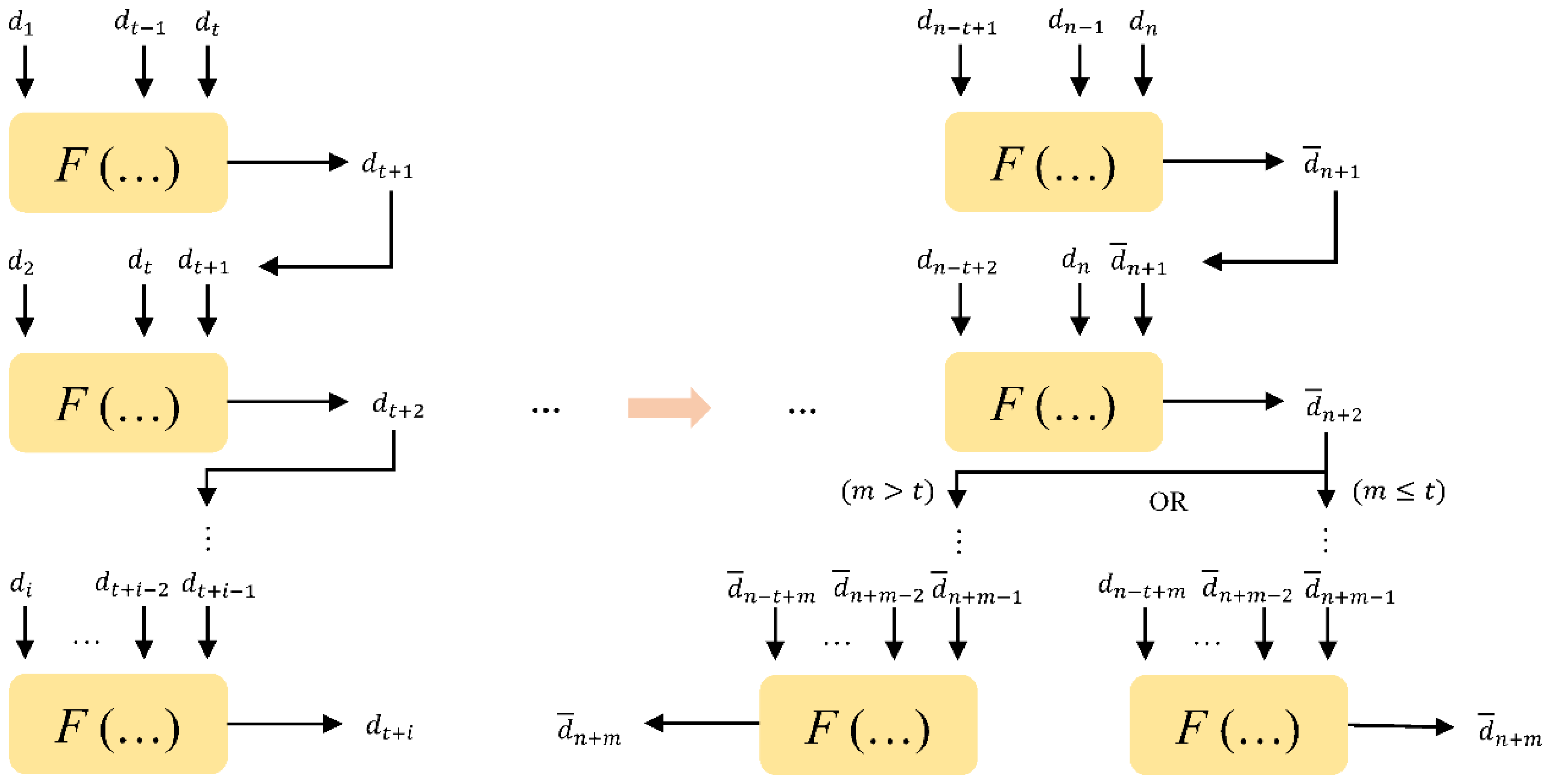
Figure 1. Intelligent analysis of tunnel surrounding rock deformation.
Jmse 10 01709 g001
Figure 2. Principle of intelligent analysis of tunnel surrounding rock deformation based on BPNN. (adapted from [36], with permission from MDPI, 2022).
Jmse 10 01709 g002
Figure 3. Intelligent prediction of neural network in tunnel surrounding rock deformation.
Jmse 10 01709 g003
Figure 4. The research methodology and process.
Jmse 10 01709 g004
Figure 5. Site selection and representative monitoring section of a coastal tunnel in South China. (a) Project area; (b) a section of the tunnel.
Jmse 10 01709 g005
Figure 6. Error curve in training process.
Jmse 10 01709 g006
Figure 7. Approximation curve after inverse transformation.
Jmse 10 01709 g007
Figure 8. The comparison curves and errors between the predicted deformation and the measured value of points A, B and C. (a) The comparison curves between the predicted deformation and the measured value of point A; (b) the comparison curves between the predicted deformation and the measured value of point B; (c) the comparison curves between the predicted deformation and the measured value of point C; (d) the errors between the predicted deformation and the measured value of points A; (e) the errors between the predicted deformation and the measured value of points B; (f) the errors between the predicted deformation and the measured value of points C.
Jmse 10 01709 g008
Table 1. Advantages, disadvantages, and applications of different methods [6,7,8,9,10,11,12,13,14,15,16,17,18,19,20,21,22,23,24,25,26,27,28,29,30,31].
Serial NumberMethodAdvantageDisadvantageApplication
1LRGood at acquiring linear relationships in the dataset; easy to operate; fast training and prediction speed.The measurement data are discrete, and the prediction accuracy is affected by complex geological conditions.It is suitable for low latitudes and there is no covariance between each dimension.
2Grayscale ModelSimple and practical; few model parameters.Little fault tolerance; not suitable for long-term forecasting.It is suitable for short-term prediction.
3SVMSimple algorithm; good robustness (in the case of small samples).Limited by the sample size; when the sample size is too large, the accuracy will be affected.It is mainly used for data classification but can also be used for regression prediction.
4TSIt allows for full consideration of the impact of seasonal and cyclical variations on specific points in time.Single linearity, stable monitoring time, equidistant data featureIt is applied to predicts related to its own previous period.
5BPNNBetter nonlinear mapping capability; better self-learning and self-adaptive capability; certain fault-tolerance capability.With low learning efficiency, slow convergence speed, and easy to fall into a local minimum stateTheoretically, it can be mapped to any function.
Table 2. Results comparison between different methods.
PointModelR2RMSEMAE
ALR0.940.940.22
TS0.991.270.29
BPNN0.990.060.01
BLR0.930.520.12
TS0.980.790.18
BPNN0.990.040.01
CLR0.880.460.11
TS0.980.550.13
BPNN1.000.010.01
Publisher’s Note: MDPI stays neutral with regard to jurisdictional claims in published maps and institutional affiliations.