Article

Numerical Study on Multiple Parameters of Sinkage Simulation between the Track Plate of the Deep-Sea Mining Vehicle and the Seafloor Soil

1
State Key Laboratory of Ocean Engineering, Shanghai Jiao Tong University, Shanghai 200240, China
2
Yazhou Bay Institute of Deepsea SCI-TECH, Shanghai Jiao Tong University, Sanya 572024, China
3
Institute of Marine Equipment, Shanghai Jiao Tong University, Shanghai 200240, China
*
Author to whom correspondence should be addressed.
J. Mar. Sci. Eng. 2022, 10(11), 1680; https://doi.org/10.3390/jmse10111680
Submission received: 28 September 2022 / Revised: 1 November 2022 / Accepted: 3 November 2022 / Published: 7 November 2022
(This article belongs to the Section Ocean Engineering)

Abstract

:
The seafloor soil is characterized by high water content, strong compressibility, and low shear strength. Deep-sea mining vehicles (DSMV) are prone to sinking when walking on the surface of the soil, which will cause significant reduction in traction performance. Therefore, it is necessary to study the sinkage performance. The track is usually considered the travelling mechanism of the DSMV, and the track plate is an important part of the movement system. The study of the interaction between the track plate and the soil is of great significance to the study of the DSMV’s sinkage performance. In this study, firstly, based on the in situ seafloor soil samples of 1000 m in a region of the South China Sea collected by a box sampler, the physical and mechanical parameters of soil were measured by indoor geotechnical instruments. Secondly, an elastoplastic soil numerical model similar to that of in situ soil was established. Based on coupled Eulerian-Lagrangian (CEL) method, a numerical model of the interaction between the track plate and soil was established. Considering the dynamic process, the structure of the track plate and the physical and mechanical properties of the soil, the numerical simulation were carried out under different conditions, such as different dynamic loading, the plate structural parameters and the soil physical and mechanical properties. It is found that the plate-sinkage curve were significantly influenced by these factors. The findings are as follows, firstly, with the increase in the pressure loading rate, the soil sinkage decreasing at the same pressure. On the other hand, with the increase in velocity, soil flow was accelerated, and the nonlinear relationship between resistance and velocity became more obvious; the L/B ratio of different track plates affects the variation law of the curve, and the maximum sinkage gradually decreases as the ratio of L/B increases; with the increase in the grouser height, the maximum sinkage gradually decreases, and the pressure-sinkage curve changes obviously with the grouser type; and different soil physical and mechanical properties affect the variation of pressure-sinkage curve. Innovatively, the heterogeneous soil stress distribution mode was obtained through the fitting function and Python secondary development. This study can provide a reference for studying the sinkage performance of the DSMV.

1. Introduction

The development of mineral resources is of great significance to the development of science and technology. Due to the earlier mining time of terrestrial mineral resources and the large amount of mining, the terrestrial resources can no longer meet the needs of human development. With the continuous exploration of the ocean by human beings, the rich mineral resources of the seafloor are becoming the new focus of competition among the world’s major economies Adapted from Ref. [1]. The deep-sea mineral resources mainly include polymetallic nodules, cobalt-rich crusts, and polymetallic sulfides Adapted from Ref. [2]. The mineral resources are rich in nickel, cobalt, copper, manganese, and other metals. The total reserves are hundreds or even thousands of times higher than those of land. The development of seafloor mining resources has formed a set of mature mining mode. The mining system includes three parts: support vessel, ore lifting pump and deep-sea mining vehicle (DSMV), as shown in Figure 1. Among them, because of the harsh seafloor environment, high water pressure, complex terrain, poor visibility, and other characteristics, so the development of the DSMV is extremely important, and the design of its structural parameters is particularly important to improve the efficiency of the ore collection and the traveling safety.
In contrast to floating remotely operated vehicles (ROV), DSMVs have a large weight in water, and the seafloor soil are characterized by high water content, low bearing capacity, and extremely thin and soft Adapted from Ref. [4]. Therefore, under the two working conditions, seafloor traveling and deploying on the seafloor, the sinkage will be too deep. Based on the heavy transport equipment on land, the track chassis with strong traction performance, small grounding pressure and high passing performance is usually used as the traveling mechanism of the DSMV in the practical engineering. On the other hand, the deep sinkage of the DSMV will bring greater static pressure sinkage resistance and bulldozing resistance when the equipment is traveling on the seafloor, which will affect the tractive performance of the DSMV. At the same time, the deep sinkage of the DSMV will also increase the difficulty of retrieval of the equipment.
As a key component of the track travelling mechanism, the track plate affects the overall motion performance of DSMVs Adapted from Ref. [3]. Therefore, it is necessary to study the influence of the track plate structure and other parameters on sinkage performance and the dynamic response of soil.
With the development of the land vehicle terramechanics, a number of studies found that the dynamic response of soil under compression can be described by the pressure–sinkage model. The sinkage experienced by the soil under a specific pressure from a certain pressure source can be quantified by the pressure-sinkage model, which can better quantitatively describe the interaction between the tracked plate and the soil under pressure. A variety of pressure–sinkage models were established by relevant scholars after a number of plate sinkage tests and theoretical analysis, as shown in Table 1. Among them, the pressure–sinkage model can be divided into theoretical and empirical models. After a number of experimental observations, the soil in earth can be roughly divided into the saturated clay and the compact sand, which can be regarded as the ideal elastoplastic materials. Therefore, the existing theoretical models were mainly based on the combination of elastic mechanics and plastic equilibrium theory. Considering some limitations in treating soil as elastoplastic material, some scholars had conducted experiments for further measurement and characterization of ground response, including the pressure-sinkage model to describe the sinkage characteristics of soil and the shear stress-displacement model to describe the traction performance of vehicle. Among them, a common method used to measure the load response of the ground surface is bevameter devices, which consists of two basic sets of tests: the plate sinkage test and the shear ring test. In the plate sinkage test, the pressure is applied to the slab by hydraulic device to make it for a period of displacement, and the change curve of the process is described by the data sampling system.
Although the above model has good adaptability in certain occasions, it is complicated to carry out the test, and the research parameters are relatively simple. In addition, the soil has the characteristics of heterogeneity in practice, and the experimental data obtained are imprecise. With the development of computer simulation technology, numerical simulation has been widely used to study the influence of more parameters on the sinkage performance of the track plate. Among them, it mainly includes two methods: finite element method (FEM) and discrete element method (DEM). M. Rashidi et al. Adapted from Ref. [20] used nonlinear FEM, the two-dimensional soil finite element model based on the Mohr-Coulomb elastoplastic material model was established by FORTRAN language, and the statistical analysis of the verification confirmed the validity of the FEM model and demonstrated the potential use of the FEM in prediction of the soil pressure sinkage behavior. Subsequently, it was modified based on this program, and a multistage load test was carried out, which was compared with the indoor plate sinkage experiment to verify the effectiveness of the FEM Adapted from Ref. [21]. A. Hemmat et al. Adapted from Ref. [22] regarded soil as a viscoelastic body, a slab sinkage model based on the FEM was established, and discussed the viscoelastic behavior of soil. By comparing with laboratory experiments, the results showed that the finite element modeling technique can be used to simulate pressure-sinkage and to predict the compressive properties. Ting Xia et al. Adapted from Ref. [23] used smoothed particle hydrodynamics (SPH) and the FEM, the numerical study of the dynamic simulation of rigid cylindric plate’s sinking process on soil was carried out by using LS-DYNA commercial software, and it had the stress distribution and flowing trend of the soil, and the simulation results show that the SPH/FEM method is useful to analyze large deformation of soil. Mojtaba Naderi-Boldaji et al. Adapted from Ref. [24] used the FEM, then, confined compression (CC), semi-confined compression (SCC) and plate sinkage (PS) numerical model were established; moreover, the pre-compression stress (σPC) which has been widely used as a criterion for assessing the susceptibility of soil to compaction was estimated.
Because some soils are soft, the large deformation will occur after the compression process, there are some defects that the study of large deformation can’t carried out by the traditional FEM. Therefore, the DEM and the coupled Eulerian-Lagrangian (CEL) method, which can effectively describe the large deformation characteristics of objects, are widely used in the numerical simulation of plate sinkage, and the DEM is more frequently used. Kju-jin Lee et al. Adapted from Ref. [25] established an experimental model of the slab sinkage based on the DEM method, and compared it with Bekker’s pressure-sinkage model to verify the effectiveness of the numerical method, and carried out sensitivity analysis of parameters such as friction coefficient and Young’s modulus. Zeinab El-Sayegh et al. Adapted from Ref. [26] founded a numerical model of circular plate sinkage based on the SPH method, and compared it with the measured data to verify the effectiveness of the numerical method. Based on the DEM, Mostafa Bahrami et al. Adapted from Ref. [27] studied the influence of different parameters on the numerical calculation results of confined compression (CC) and plate sinkage (PS), and experimental verification was carried out. At the same time, it was pointed out that the difference between the actual soil particle size and the DEM simulated particle size was large, resulting in a significant difference in the numerical calculation results. Thus, it is necessary to study the proportional relationship between DEM parameters and particle size. K. Amudha et al. Adapted from Ref. [28] described the large deformation characteristics of soil under plate motion based on the CEL method, and the experimental results of plate sinkage under different working conditions were studied. However, the difference between the CEL method and experiments was not compared, and the numerical simulation of multiple working conditions was not carried out in detail, so only the deformation characteristics of soil were obtained.
As can be seen from the above literature research, many researchers have set up a plate sinkage numerical model based on different numerical methods, and the validity of the numerical method was verified which compared to the experimental result. However, the curve variation law of pressure-sinkage model was further discussed, and the study parameters were relatively simple. In the study of sensitivity parameters, such as the soil physical-mechanical properties, the form of the external load is less.
Considering that the numerical simulation parameters of the plate sinkage test in the above literature were relatively simple, a study on the sinkage interaction of the track plate and the seafloor soil under multiple parameters based on the CEL numerical method was carried out in this study. Firstly, the physical and mechanical parameters were obtained from in situ seafloor undisturbed soil samples using indoor geotechnical instruments. Based on the physical and mechanical properties of soil and the CEL numerical method, a numerical model of the track plate-seafloor soil sinkage interaction was established. The pressure-sinkage curve was obtained from the model. Then, the numerical simulation was carried out under different cases such as the dynamic process, the track plate structure, and the soil’s physical and mechanical properties. On the other hand, ABAQUS secondary development based on the Python platform was carrier out in this paper, the heterogeneous material of soil Eulerian unit was established innovatively, and preliminarily discussed the pressure-sinkage model under heterogeneous soil compared with homogeneous soil. Different from the traditional experimental method, in this study, the CEL method was used to study the multi-parameter sinkage interaction between the track plate and the seafloor soil. It provides new insights into studying the sinkage performance of deep-sea mining vehicles.

2. Numerical Model of the Single-Track Plate–Soil Sinkage Interaction

2.1. Numerical Methods

CEL method was first proposed by Noh Adapted from Ref. [29], and further improved by Benson and Okazawa Adapted from Ref. [30], which was embedded in the finite element software ABAQUS. This method overcomes the defects of Lagrangian method and Eulerian method. The Lagrangian method and Eulerian method are shown in Figure 2. In the analysis of the coupling effect between the seafloor soil and structure, the Eulerian algorithm is used for the soil, that is, the mesh is fixed, the soil can flow in the mesh, and there is no mesh distortion. The structure adopts Lagrangian algorithm, which is used to calculate the stress field of the soil and the displacement or reaction force of the structure at any time. The changes of the contact surface between the soil and structure are tracked through the boundary of the structure. Briefly, the contact surface between the structure and the soil is tracked by the Lagrangian body, so that the Lagrangian body occupies the void region inside the Eulerian mesh, ensuring that the Lagrangian body and the Eulerian body never coincide in physical space. Therefore, it can be seen that the most important thing in CEL method is the flow of material inside the mesh. The flow model is described by the Eulerian flow control conservation equation, which is as follows [29]:
ρ t + ( ρ v ) = 0 ,
ρ v t + ( ρ v v ) = σ + ρ b ,
e t + ( e v ) = σ D .
where ρ is the density, v is the material velocity, σ is the Cauchy stress, b is the body force, and e is the internal energy, and D is the velocity strain.
At the same time, a dynamic explicit analysis method was adopted in the numerical model. Explicit dynamic analysis can be used to analyze complex contact problems involving the interaction of multiple independent objects. At present, CEL method has been widely used to analyze the large deformation problem of soil and structure coupling. For example, the heave and movement of the seafloor soil are caused by penetration, traction, anchor dragging, and anchor dropping of marine structures. The CEL method has been applied in the research on track plate–seafloor soil interaction.

2.2. The “Pioneering-I” DSMV, Track Mechanism and Track Plate Model

This section introduces the DSMV structure and the track plate parameters which are used in numerical model. The overall structure of “Pioneering-I” DSMV, designed by Shanghai Jiao Tong University, is depicted in Figure 3a. The entire model is composed of a track mechanism, hydraulic system, observation system, ore-collecting mechanism, buoyant material, lifting mechanism, electric control system, positioning navigation system, and attitude control system.
The main structural parameters of the DSMV are listed in Table 2. The details of the track mechanism of the DSMV are shown separately in Figure 3b. The T-shaped track plate is illustrated in Figure 3c. The grouser height is 0.05 m and the thickness is 0.015 m.

2.3. The Soil Numerical Parameters Obtained from Physical and Mechanical Tests

The physical and mechanical properties of the seafloor soil are obviously different from those of terrestrial, so it is very important to obtain the characteristics of the in situ sample. In this section, the physical and mechanical characteristics of the collected in situ seafloor soil were studied to obtain important mechanical parameters for establishing the numerical model, which provides data support for the study of the interaction between the track plate and the soil sinkage.
In Figure 4, In July 2021, a box sampler was used to collect three columnar samples in the South China Sea, with water depths of 188 m (J1), 208 m (J2), and 1000 m (J3), corresponding to the location of the DSMV deployment. Owing to the limitation of the sampling tube length, the sampling lengths were 45, 50, and 43 cm. According to visual observations and penetration tests of the samples, the soil was thin and soft, similar to mud.

2.3.1. Physical Test Analysis

As can be seen from Table 3, the value of the soil including moisture content, porosity ratio, saturation, and liquidity index (IL) are relatively high. Therefore, the soil is relatively soft and exhibits high liquidity. On the other hand, the moisture content, natural void ratio, and liquidity index decreased with increasing depth, whereas the density and saturation increase with increase in depth. According to the data listed in Table 4, the soil mainly comprises silt and clay, and the type is clayey silt. The types in the three stations remain unchanged vertically.

2.3.2. Mechanical Test Analysis

Figure 5 shows photos of the laboratory tests, including penetration resistance, shear strength tests, and consolidation tests. Direct shear and cross plate shear were used in the shear strength test. The former was used to obtain the cohesion and internal friction angle of the soil while the latter was for the maximum shear strength.
The physical and mechanical properties of 1000 m depth soil in the South China Sea were obtained by testing and sorting the experimental data, as indicated in Table 5.
Through the analysis of the mechanical properties, it was found that the seafloor soil is saturated clay with high water content. The water content gradually decreases from the surface, the soil becomes hard from soft, and the bearing capacity gradually increases. The shear strength of the surface soil is low, and the maximum value is only 5 kPa. Thus, the DSMV can easily slip when moving. However, the surface soil has strong compression properties, and the DSMV can easily sink.

2.4. Computational Domain and Initial Parameter Setting

Based on CEL numerical method, the Lagrangian track plate and Eulerian soil were established, respectively. The soil was regarded as an ideal elastoplastic body, which can use Mohr-Coulomb constitutive model includes linear elastic model and Mohr-Coulomb Plastic yield criterion to describe the elastoplastic characteristics of soil. The track plate model was set as a rectangle slab without the grouser, and its structure sizes were consistent with the “Pioneering-1” DSMV, with a length of 0.6 m, a width of 0.15 m and a thickness of 0.02 m. The soil model was set as a cuboid, and the size of the computational domain needs to be analyzed.
In Figure 6, The soil model was divided into two parts, including the soil and the void region, among them, a void layer was set above the soil model to capture the soil surface rising during the track-plate motion process. On the other hand, the void region is also to avoid the soil being lifted beyond the boundary of the model and causing the calculation result not to converge. the latter was used to describe the deformation and uplift of the soil, where the void layer height was set to 0.4 m. In addition, the overall height of the soil was calculated according to Equation (4). Based on Bekker’s theory of soil stress transfer, the empirical equation of the soil stress transmission is as follows Reprinted from Ref. [31]:
σ z = p [ 1 z 3 ( z 2 + r 2 ) 3 2 ]
wherein, σz is the soil stress at the depth z, p is the surface pressure of the plate, and r is the half of the track plate length.
As the maximum length of the initial plate is 0.6 m, the Equation (4) shows that when z is 2 m and r is 0.3 m, the stress σz at the bottom is close to zero and the stress transfer can be ignored. Therefore, the overall soil height H was set to 2 m. To eliminate boundary effects, both length and width were set to 2.5 m.
Furthermore, for the purpose of subsequent mesh sensitivity analysis, the initial parameter setting of the model needs to be completed, including soil physical and mechanical properties parameters, motion conditions, soil boundary, and external load conditions.
According to the in situ sampling data and the conditions set by the elastoplastic soil, the soil physical and mechanical properties parameters are shown in the Table 6. Among them, the shear strength is 5 kPa, and the elastic modulus was set to 500 times the shear strength Adapted from Ref. [32], in addition, according to the literature research on the physical characteristics of the seafloor soil, the Poisson’s ratio was set to 0.49Adapted from Ref. [33].
On the other hand, the boundary conditions of the overall numerical model were set as follows:
  • Velocity setting value: 0.05 m/s in the vertical direction. Moving for 5 s with constant velocity, and realizing 0.25 m displacement.
  • Eulerian volume percentage (EVP): The initial setting of the soil EVP was 100%, and the void region was set to 0.
  • The horizontal displacements of the four sides of the soil model and the six degrees of freedom of the bottom surface were restricted. The surface hydrostatic pressure at the top of the soil was set to simulate seawater pressure. The seawater depth was set as 1000 m, thus, the hydrostatic pressure was 10 MPa.
  • The gravity field was applied to the overall soil model and the geostatic stress was preset.

2.5. Geostatic Stress Balance

Since there is gravity in the numerical model of soil, the initial geostatic stress balance of soil should be carried out first when the track plate-soil model is established, to make sure that there is an initial stress and no initial vertical displacement in the soil.
Since the Mohr-Coulomb constitutive model was adopted in this numerical model, it is difficult to converge with the automatic balance module of ABAQUS. Therefore, it is necessary to carry out the geostatic stress balance by using “.ODB” file importing method. Determining conditions for success of geostatic stress balance are as follows:
(1)
The vertical displacement of the soil model is zero or very small, generally at least 10−6 m.
(2)
The internal stress of soil exists.
After importing the “.ODB” file for many times, it can be seen from the Figure 7 that there is internal stress S33 in the soil, but the vertical displacement U3 is very small. The model obtains a good effect of geostatic stress balance, and the vertical displacement after balance reaches the order of 10−6–10−7 m, which meets the accuracy requirements.

2.6. Sensitivity Analyses of Mesh Parameters

Eulerian and Lagrangian mesh should be set up for the simulation parts, respectively, when the numerical calculation based on CEL method is carried out. As for this numerical model, the track plate is regarded as a rigid body, so according to the finite element theory, the Lagrangian mesh part is not deformed, and only the mesh sensitivity analysis of the Eulerian model of the flow is needed. In order to ensure the calculation accuracy, four sets of mesh seeds were set in the model, and the mesh type was hexahedral mesh. The soil mesh topology is dense in the middle and relatively sparse around, as shown in the Figure 8. The soil mesh was set to EC3D8R unit. The track plate mesh used eight-node Lagrangian element C3D8R.
The sensitive analysis parameters were set, as presented in Table 7.
In the Figure 9, the soil resistance of the track plate solved by the numerical model under the same velocity condition and different meshes were obtained. Through the analysis of the curve results, it can be seen that different mesh sizes have great differences in numerical calculation results. Among them, the mesh seed layout affecting the numerical calculation results from the largest to the smallest are zone-3, zone-2, and zone-1, respectively. Furthermore, by analyzing the convergence of the resistance values of each curve, and the curve group with good convergence was obtained. The set of values at which the values start to converge was selected as the final mesh value selection of the calculation area. the numerical mesh size parameters were obtained in Table 8.
The overall and local mesh distributions are illustrated in Figure 10. The overall mesh quantity was 202,500.

3. Results and Discussion

In this section, based on the established numerical model, the numerical simulation was conducted on the interaction between a single track plate and the soil with different parameters, including different loading conditions, the plate structures, and soil parameters.

3.1. Different Loading Conditions

3.1.1. Different Pressure Loading Conditions

In the plate sinkage experiment, the hydraulic mechanism was used to apply pressure to the surface of the track plate, and the curves of different loading pressures and sinkage are measured. However, there is little research on the difference of curves under different loading rates. In this section, the dynamic responses of the soil under compression under different pressure loading rates were carried out, the schematic is shown in Figure 11a. Figure 11b shows the curve of pressure load variation with time, representing the working conditions with different loading rates under the same pressure loading interval. The pressure loading interval was set from 0 kPa to 100 kPa. Among them, k is the slope of the line in the Figure 11b, which represents different pressure loading rates.
Figure 12a shows the relationship between the soil sinkage and pressure under different pressure loading rates. As can be seen from the figure, the difference of sinkage caused by different dynamic external loads can effectively described by numerical simulation. As can be seen from Figure 12a, as the loading rate slows down, the sinkage of the slower loading rate is larger under the same pressure. From the perspective of soil properties, the slower loading rate makes the track plate in direct contact with the soil for a long time, and the soil response is more adequate. Then, at the same pressure, the soil disturbance is larger. It can also be found from the figure that the inflection point of the decline of the pressure-sinkage curve is advanced when the loading rate is small, and the soil plastic failure occurs at that moment. On the other hand, in the initial pressure loading stage, the soil deformation trend is basically the same, indicating that the deformation characteristics of soil affected by the rate of the pressure loading have little difference in this time.
Figure 12b shows the relationship between the maximum sinkage of soil and the loading slope k after reaching 100 kPa. It can be found that with the increase in slope k, the maximum sinkage gradually decreases, and the overall curve presents nonlinear variation characteristics. On the other hand, with the increase in pressure, the variation of maximum sinkage becomes more obvious, indicating that the loading rate has a great influence on the sinkage. Therefore, the pressure-sinkage curve is a dynamic model that changes with time, and the influence characteristics of dynamic factors are obvious.
Figure 13 compares the analogy between the numerical simulation in Figure 13a and the plate sinkage experiment, which is shown in Figure 13b, and it can be found that the curve trends of the two are similar. Take the case k = 5 as an example, the curve can be divided into three stages. The first stage presents elastic deformation, and the second stage is transition stage where elastoplastic deformation occurs. In the third stage, plastic deformation occurs, and the rise in the curve slows down. It can also be seen from Figure 13b that when the slope k becomes small, the soil deformation enters the plastic change area earlier.

3.1.2. Different Velocities

Another dynamic process was considered in this section, that is, the dynamic response of soil when the track plate sinks at a constant velocity was studied. The schematic is shown in Figure 14a. The studied parameter is the sinkage velocity of the track plate. When the track plate is at a constant velocity, the resultant force is zero, and the soil resistance is equivalent to the external force on the upper surface of the track plate. Figure 14b shows the curve of sinkage variation with time. At the same time, the total displacement was controlled to be 0.8 m. The velocities of the four groups of working conditions were set as 0.02, 0.04, 0.08, and 0.16 m/s, respectively.
Figure 15 shows the variation curves of resistance with displacement at different velocities. It can be seen from the figure that the velocity affects the resistance in the process of the soil sinkage, but the influencing factors are smaller than the pressure loading rate. After further analysis of the data, it can be found that the force of the track plate is different under the same displacement, especially in the displacement district 0–0.1 m. On the other hand, all resistance curves show a small upward trend when reaching to a certain displacement. The trend of resistance variation is divided into two stages. In the first stage, the resistance increases faster. When the external force is applied to the soil, the strength of the soil increases rapidly due to the action of compaction, and the dynamic response is obvious. Then, after reaching a certain displacement, the curve enters the second stage. In the second stage, the resistance increases slowly. With the increase in sinkage, the soil bearing capacity at the bottom of the track plate gradually increases, and the trend of resistance increasing decreases gradually.
On the other hand, it can be seen from the figure that as the velocity increases, the displacement value corresponding to the inflection point of the resistance curve from the first stage to the second stage gradually increases. In addition, in the first stage, the resistance at the same displacement is negatively correlated with the velocity. In the second stage, the higher the initial velocity, the higher the resistance value. However, with the progress of displacement, the internal soil flow is accelerated, the response is more complex, and the nonlinear relationship between resistance and velocity is more obvious.

3.2. Different Track Plate Structures

In the plate sinkage experiment, considering that the ground surface of different vehicles includes rectangles, circles, and ovals, it is necessary to use rectangles with various length-width ratios, circles with different diameters and oval plates with different eccentricities to obtain the predicted data with maximum reliability. Therefore, it is necessary to study the pressure–sinkage model of different shaped plates. In this study, rectangular with different aspect ratios and circle plate with different diameters were compared to obtain the differences of the pressure–sinkage models under different shape plates.

3.2.1. Different L/B Ratios

In this section, four track plates with different length-width (L/B) ratios were selected to carry out research on soil dynamic response of the tracked plate under different L/B ratios. In Figure 16, the L/B ratio was set to 1.5, 2, 3, 4, 6, and 8. Among them, the length was set to be 0.6 m, which is the same as the track plate of the “Pioneer-I” DSMV. On the other hand, the pressure load applied varies from 0 kPa to 100 kPa, with slope k value is 10.
It can be seen from Figure 17a that the L/B ratio is an important factor affecting the soil sinkage under the same pressure load condition. In addition, as the ratio of L/B increases, the maximum sinkage gradually decreases. The reason is that under the same length of the track plate, the width has a greater influence on the soil and the soil disturbance is more obvious. Therefore, the inflection point of plastic deformation and failure is early, and the internal soil plastic flow occurs prematurely.
Figure 17b shows the relationship between the maximum sinkage of the soil at 100 kPa and L/B ratios. In this section, the fitting equation of the maximum sinkage and L/B ratios of the track plate of the “Pioneering-I” DSMV was established, as shown in Equation (5).
Maximum   Sin kage = 0.1 + 1.55 e ( L / B ) / 2.7
Further, in order to verify the correctness of the equation in the numerical simulation, the sinkage performance of L/B = 5 and 10 was studied. As can be seen from the Table 9, the equation prediction was relatively accurate in L/B = 5 and 10.
In this section, the numerical simulation under different L/B ratios was further studied. The relationship between sinkage (S)/B and different pressure was obtained by normalizing the sinkage and the track plate width. It can be found from the Figure 18a that for the elastoplastic soil, all curves basically overlap except L/B is 1.5. It is shown that under different L/B ratios, the relationship between the ratio of the sinkage to the width of the plate and the pressure remains unchanged. The numerical results are consistent with those in the literature [18], which verifies the effectiveness of the numerical method. On the other hand, as can be seen from the Figure 18b, with the increase in the L/B ratio, the maximum S/B value gradually converges, and when the L/B ratio is greater than six, the value basically remains unchanged.

3.2.2. Comparison between the Rectangle Plate and the Circle Plate

Adapted from Bekker [34] systematically discussed the plate size effect affecting the results of pressure-sinkage curve. In Figure 19, Through a number of experiments, it was found that the sinkage variations of the plate with a larger L/B ratio and the circular plate with the corresponding width as the diameter (D) were basically the same under the same pressure load. Based on the above experimental results, this section verifies the results based on numerical calculation. Based on plates in Section 3.2.1 with different L/B ratios, circular plates with different widths as diameters were designed at the same time, and a comparison between the two working conditions was obtained. As can be seen from the Figure 20a, when the L/B ratio is large, it is consistent with the results of Bekker’s research, and when the ratio is small, there will be a big difference. Furthermore, the pressure-sinkage curves of the rectangular plate and the circle plate under the same pressure are extracted under the conditions of L/B of 6 and 8. As can be seen from the Figure 20b, the curves of the two curves are highly consistent, which further proves Bekker’s experimental theory.
Meanwhile, Figure 21 shows the curve of the soil sinkage under different circular plate diameters. It can be seen from the figure that, with the increase in circular plate diameter, the maximum sinkage gradually decreases, which is the same as that of rectangular plate. Larger diameter has greater influence on soil and more obvious soil disturbance, and soil plastic flow occurs prematurely.
Similar to the rectangular plate, the diameter of the circle plate and the sinkage was normalized in this section, and the relation curve between different pressures and S/D is obtained. It can be found from the Figure 22a, different from the rectangular plate, the relationship between the ratio of the sinkage to the plate width and the pressure varies greatly under different diameters. On the other hand, it can be seen from the Figure 22b that the relationship between the plate diameter and the maximum sinkage is nonlinear with no convergence phenomenon. Comparing with the data of the rectangular plate, the normalized data results of rectangular plate and circular plate are different. Therefore, the calculation results of a rectangular plate and a circle plate cannot be completely equivalent.

3.3. Different Grouser Structure Parameters on the Single Track Plate

Because the seafloor soil is relatively thin and soft, the DSMV is prone to slipping and sinking when traveling. It is usually necessary to increase the height or change the type of the grouser to obtain better traction performance of the DSMV. On the other hand, changing the structural parameters of the grouser will also affect the sinkage performance of the DSMV, but there is little research in the existing literature. In this section, the pressure-sinkage performance of the track plate with different grouser height and type was studied.

3.3.1. Different Grouser Height

In this section, four groups of different grouser height were simulated. The grouser height was set to 0.05 m, 0.1 m, 0.15 m, and 0.2 m. At the same time, the rectangle plate was designed as the control group.
It can be seen from the Figure 23a that with the increase in the height of the grouser, the maximum sinkage of the soil gradually decreases. However, considering that higher grouser will bring more resistance and reduce the traction performance of the DSMV, it is necessary to comprehensively consider the height setting of the grouser combined with the traction performance of the DSMV. The Figure 23b shows the variation of the maximum sinkage at different grousers. It can be seen from the figure that the maximum sinkage is linearly related to the height of the grouser.

3.3.2. Different Grouser Types and Numbers

The grouser shape is also an important factor affecting the traction performance of the DSMV. In this section, the pressure-sinkage model difference was studied under different grouser types and numbers. The grouser shape was shown in Table 10. The grouser was set to Triangular-shaped (Tri-shaped), Parabola-shaped, T-shaped, and taking T-shaped as the research object, the influence of different number of grousers were studied. At the same time, a rectangle slab without grouser was added as a control group. Among them, the grouser height was set to a same value, 0.1 m.
It can be seen from the Figure 24 that the influence factors of different grouser shapes and numbers are obvious. In particular, under the same pressure, the rectangle has a larger disturbance to the soil, and the soil has a larger plastic deformation and flow, so the sinkage is the largest. The maximum sinkage from small to large are triple grousers, double grousers, parabola grouser, single grouser, triangle grouser and rectangle slab without grouser. In theory, when the track plate with three grousers is subjected to external pressure, the bottom of the grouser and the soil contact area is large. In addition, the soil becomes hard under pressure and the soil carrying capacity increases, so the sinkage is the lowest.

3.4. Different Soil Parameters

In the previous section, the influence of different dynamic loading factors and structural parameters of the track plate on the relationship between the pressure and the soil sinkage was studied. The studied parameters are not related to the soil itself, but in the actual process, there will be the following situations.
(1)
The actual seafloor soil is not completely homogeneous, and its physical and mechanical properties change with time and space.
(2)
The physical and mechanical properties of the seafloor soil in different regions are not completely the same.
(3)
In the experiment of the plate-sinkage tests tank, the simulated soil needs to be configured in the soil tank at a certain height, so the influence of different soil tank height on the pressure-sinkage model.
The above conditions are related to the soil itself, so it is necessary to study the influence of different soil parameters on the pressure-sinkage model. Therefore, sensitivity analysis of different soil parameters were carried out in this section considering the above three cases, respectively.

3.4.1. Different Soil Height

In this section, the influence of different soil height on the pressure–sinkage model was studied. The height of soil tank was set as 0.25 m, 0.5 m, 0.6 m, 0.75 m, 1 m, 1.5 m, 2 m, and 3 m.
By analyzing the data in Figure 25a, we found that different soil height had a great influence on the parameters of the pressure-sinkage model. This is because the lower the height of the tank, the soil at the bottom of the tank cannot fall under the action of pressure, and the bottom of the tank provides a support force opposite to the direction of movement, which improves the local soil carrying capacity. Therefore, the smaller the height, the smaller the displacement under the same load. In the actual experiment, this factor should be considered, which will cause the inflection point lag of plastic failure, resulting in experimental error. Numerical simulation can determine the optimal soil tank height to increase the experimental effectiveness. Figure 25b shows the relationship between different soil height and maximum sinkage. It can be found that, with the increase in height, when the height is between 1 and 1.5 m, the maximum sinkage basically remains unchanged. The relationship between soil height and maximum sinkage is linear until the soil height is less than 1 m.

3.4.2. Different Soil Mechanical Properties

Since the soil was set as an elastoplastic soil, the elasticity was set as a linear elastic model, and the plasticity followed the Mohr-Coulomb plasticity criterion. Therefore, elastic modulus, cohesion, and internal friction Angle are the main influencing parameters of the numerical model of pressure-sinkage, and the three parameters were studied separately in this section. The values of the study parameters are shown in the Table 11.
(1)
Internal friction angle (IFA)
As can be seen from the Figure 26, with the increase in the IFA, the sinkage of soil gradually decreases under the same pressure. This is because the friction between soil particles is large with the increase in IFA. At this time, the soil is similar to sandy soil, showing a larger bearing capacity and relatively hard characteristics, so the soil sinkage is little.
(2)
Cohesion
As can be seen from the Figure 27a, the influencing factors of cohesion are obvious. When the cohesion is 5 kPa, the soil is relatively thin and soft, reflecting obvious deformation characteristics under compression. The maximum sinkage at 100 kPa is several times more than that in other groups of working conditions. From 10 kPa, the maximum sinkage of soil gradually converges. With the increase in cohesion, soil viscosity increases, at this time, the soil is more compact. Therefore, under the same pressure, the sinkage becomes smaller gradually.
(3)
Elasticity modulus (E)
Since the soil is set as an elastoplastic body, the elastic modulus plays a great role in the elastic deformation stage. As shown in the black curve in Figure 28a, when E = 20 MPa, the elastic modulus of soil is small, and the soil is prone to large elastic deformation. Under the same internal friction angle and cohesion, the soil is prone to plastic deformation earlier, and is more likely to be disturbed to plastic flow. In general, the increase in elastic modulus is inversely proportional to soil sinkage, and the maximum soil deformation gradually converges with the increase in elastic modulus.

3.4.3. Heterogeneous Soil Varying with Depth

All the above studies are homogeneous soils with the same physical and mechanical properties in space. In fact, in situ sampling tests of seafloor soil shows that physical and mechanical properties change with depth. Specifically, the water content gradually decreases, and the soil gradually becomes hard. At the same time, it shows the characteristics from soft clay to clay and then to sand. Therefore, it is necessary to study the relationship between the track plate and sinkage under the soil numerical model where the physical and mechanical properties vary with depth.
In order to achieve a wider range of soil research applications, five groups of control tests to carry out numerical analysis were set up. Among them, the changing factors of physical and mechanical properties are IFA, cohesion, and density, and the study variables do not consider the deformation characteristics of the elastic stage. Each parameter was set as follows in Figure 29, and the corresponding fitting function is shown in the Table 12. Among them, there are three different functional relationships, linear, exponential, and logarithmic, respectively, which can describe the different changes of physical and mechanical properties with depth. The depth direction was defined as the analytical function variable by the analytical field in ABAQUS, and five mechanical property curves varying with depth were fitted by using different functional relationships. Based on the five soil models, the pressure-sinkage study was carried out under the same pressure loading conditions. Table 13 shows the simulation case name and corresponding physical and mechanical parameters label.
In Figure 30, it can be found that under the same pressure, the difference of different curves is more obvious. When the mechanical properties change rapidly at first and then slowly with depth, the sinkage changes slowly. On the contrary, the plastic flow in the soil occurs prematurely in the nolinear-4 case. It can also be seen from the figure that as the pressure reaches 120 kPa in the nolinear-4 case, the curve gradually becomes concave, which reflects the compaction of the soil. This is because the physical and mechanical properties in the early stage of pressure load do not change significantly with depth, and the characteristics of pressure and sinkage are similar to those of homogeneous soil. As the mechanical properties change greatly with depth, the soil is disturbed significantly, and the effect of compaction is obvious. Therefore, in laboratory experiments, it is important to mix soil with different mechanical properties in different depths to better represent the actual seafloor conditions.

3.4.4. Heterogeneous Soil in Three Dimensions Space

In seafloor, the physical and mechanical properties of soil not only change with depth, but also exhibit different properties in the horizontal direction. Therefore, it is necessary to establish a soil model that can describe the heterogeneous characteristic in three dimensions. In this section, through the secondary development of ABAQUS commercial software, the establishment of heterogeneous soil model of Eulerian element under large deformation characteristics was carried out. The soil model in ABAQUS was configured with heterogeneous material properties based on Python language, and the numerical simulation of soil sinkage was carried out based on the numerical model. In the existing literature, most of the Lagrangian materials were set to be heterogeneous, but the Eulerian materials with large deformation are rarely discussed. Figure 31 show the flow charts of heterogeneous soil generation of Lagrangian and Eulerian bodies, respectively. It can be seen that the two have obvious differences in random material generation. Eulerian random material generation is more complex.
In this section, a heterogeneous Eulerian soil model was established according to the flow chart as shown in Figure 32b. The soil model was divided into three parts, as shown in the Figure 32a: the void region, heterogeneous soil, and homogeneous soil. The density range was set to 1000–2200 kg/m3, the internal friction angle range was set to 1–25°, and the cohesion range was set to 2–30 kPa. Heterogeneous soils include a mixture of soft clay, clay, and sand. Figure 32b shows the density distribution contours. It can be seen that the establishment method of heterogeneous Eulerian soil model proposed in this study is effective.
Based on the numerical model of heterogeneous soil, the pressure–sinkage model was studied under the same condition of pressure load rate; in this section, the pressure load range is 0–120 kPa, and the loading slope k is 30. It can be found from Figure 33a that heterogeneous soil and homogeneous soil exhibit completely different characteristics of sinkage. For heterogeneous soil in Figure 33b, the elastic deformation occurs quickly in 0–20 kpa, and the soil sinkage remains basically unchanged at about 20 kPa. At this time, the bearing capacity of the soil is large, and the pressure load is not enough to make the soil sinkage.
Figure 34 shows the internal stress distribution of soil under three conditions: homogeneous soil, physical and mechanical properties varying with depth, and heterogeneous soil. Among them, the pressure loading rate remains the same, and the sinkage of homogeneous soil and soil whose physical and mechanical properties vary with depth remain the same. It can be seen from the figure that the soil stress contour of homogeneous soil and the physical and mechanical properties changing with depth are basically similar, and the stress core is formed inside the soil and gradually expands outward. However, for heterogeneous soil, the distribution of internal physical and mechanical properties is not consistent in space, so when the plate moves vertically, the internal disturbance of soil is disordered, and irregular stress distribution characteristics are formed. It can be seen from the analysis of stress contours that the nonlinear response of heterogeneous soil is more complex after the pressure load process.

4. Conclusions

In this paper, an elastoplastic numerical model of seafloor soil was established based on in situ data. the numerical simulation of the plate sinkage was carried out under different conditions, such as different dynamic loading, velocities, the plate structural parameters, and soil physical and mechanical properties. In addition, the influence of different parameters on the dynamic response of the sinkage interaction between the track plate and soil was obtained. The main research conclusions are as follows:
(1)
The change of dynamic parameters affects the pressure-sinkage curve. The dynamic parameters studied include loading rate and velocity. With the increase in the pressure loading rate, the soil sinkage decreasing at the same pressure. The overall curve shows three stages: elastic deformation, transition and plastic failure. On the other hand, with the increase in velocity, soil flow was accelerated, and the nonlinear relationship between resistance and velocity became more obvious.
(2)
Considering the single plate and soil interaction, the analysis of plates with different L/B ratios shows that the maximum sinkage gradually decreases as the ratio of L/B increases. On the other hand, when the ratio of L/B is larger, the results are consistent with those of circular plates with the same width as the diameter.
(3)
With the increase in the grouser height, the maximum sinkage gradually decreases, and the maximum sinkage changes linearly with the grouser height. On the other hand, under the same pressure load, the maximum sinkage from small to large is triple grousers, double grousers, parabola, single grouser, triangle and slab without grouser.
(4)
The influence of soil physical and mechanical properties was studied. The elastoplastic characteristic parameters of different soil types, including elastic modulus, cohesion and internal friction angle, have obvious influence on the pressure–sinkage curve. In addition, with the increase in the three parameters, the soil sinkage becomes smaller.
(5)
The influence of nonlinear characteristics of soil was studied. Based on the analytical field and the secondary development of the ABAQUS, the two numerical model of heterogeneous soil was established. Moreover, the pressure-sinkage model was further studied, and it is found that the characteristics of the model are quite different from those of the homogeneous soil.

Author Contributions

P.S.: Conceptualization; methodology; software; validation; formal analysis; resources; data curation; writing—original draft; writing—review and editing; supervision, project administration; funding acquisition. H.L.: Software; validation; formal analysis; data curation; writing—original draft; visualization. J.Y.: Methodology; software; validation; investigation; visualization; writing—review and editing. L.D.: Software; validation; writing—review and editing. M.L.: Software; validation; writing—review and editing; S.L.: Software; validation; writing—review and editing. All authors have read and agreed to the published version of the manuscript.

Funding

This study was supported by the State Key Laboratory of Ocean Engineering. This work was also supported by the Science and Technology Committee of Shanghai Municipality (19DZ1207300), Major Projects of Strategic Emerging Industries in Shanghai, and Natural Science Foundation of Hainan Province (520LH015).

Informed Consent Statement

Informed consent was obtained from all subjects involved in the study.

Data Availability Statement

Not applicable.

Acknowledgments

The authors would like to thank the anonymous reviewers for their constructive suggestions which comprehensively improve the quality of the paper.

Conflicts of Interest

The authors declare no conflict of interest.

References

  1. Sharman, R. Deep-Sea Mining. 2017. Available online: http://www.onacademic.com/detail/journal_1000039884676810_7aff.html (accessed on 9 November 2021).
  2. Leng, D.; Shao, S.; Xie, Y.; Wang, H.; Liu, G. A brief review of recent progress on deep sea mining vehicle. Ocean Eng. 2021, 228, 108565. [Google Scholar] [CrossRef]
  3. Xu, F.; Rao, Q.; Ma, W. Track shoe structure optimization of deep-sea mining vehicle based on new rheological calculation formulae of sediment. Mech. Based Des. Struct. Mach. 2019, 47, 479–496. [Google Scholar] [CrossRef]
  4. Yamazaki, T.; Komine, T.; Kawakami, T. Geotechnical properties of deep-sea sediments and the in-situ measurement techniques. In Proceedings of the Sixth ISOPE Ocean Mining Symposium, Changsha, China, 10–13 October 2005; OnePetro: Richardson, TX, USA, 2005; pp. 48–55. [Google Scholar]
  5. Boussinesq, J. Application des Potentiels à l’Étude de l’Équilibre et du Mouvement des Solides Élastiques: Principalement au Calcul des Deformations et des Pressions que Produisent, dans ces Solides, des Efforts Quelconques Exercés sur une Petite Partie de Leur Surface; Gauthier-Villars: Paris, France, 1885. [Google Scholar]
  6. Terzaghi, K. Theoretical Soil Mechanics; Chapman and Hali, Limited John Wiler and Sons Inc.: New York, NY, USA, 1994. [Google Scholar]
  7. Ageikin, J.S. Off-the-Road Wheeled and Combined Traction Devices: Theory and Calculation; Amerind Pub. Co.,: New Delhi, India, 1987. [Google Scholar]
  8. Ageikin, J.S. Off-the-Road Mobility of Automobiles; Amerind Pub. Co.,: New Delhi, India, 1987. [Google Scholar]
  9. Bernstein, R. Probleme zur experimentellen Motorpflugmechanik. Der. Mot. 1913, 16, 199–206. [Google Scholar]
  10. Saakyan, S.S. Vzaimodeistrie Vedomogo Kolesa i Pochvi; 1959. [Google Scholar]
  11. Tsytovich, N.A. Soil Mechanics; Gosstroizdat: Moscow, Russia, 1963. [Google Scholar]
  12. Hegedus, E. Plate sinkage study by means of dimensional analysis. J. Terramech. 1965, 2, 25–32. [Google Scholar] [CrossRef]
  13. Onafeko, O.; Reece, A. Soil stresses and deformations beneath rigid wheels. J. Terramech. 1967, 4, 59–80. [Google Scholar] [CrossRef]
  14. Bekker, M.G. Introduction to Terrain-Vehicle Systems. Part I: The Terrain. Part II: The Vehicle; University of Michigan: Ann Arbor, MI, USA, 1969. [Google Scholar]
  15. Youssef, A.-F.A.; Ali, G.A. Determination of soil parameters using plate test. J. Terramech. 1982, 19, 129–147. [Google Scholar] [CrossRef]
  16. Wong, J.; Radforth, J.; Preston-Thomas, J. Some further studies on the mechanical properties of muskeg in relation to vehicle mobility. J. Terramech. 1982, 19, 107–127. [Google Scholar] [CrossRef]
  17. Sargana, M.; Gee-Clough, D.; Gupta, C. A dynamic equation for the pressure-sinkage relationship in saturated clay soils. J. Terramech. 1985, 22, 111–120. [Google Scholar] [CrossRef]
  18. Gotteland, P.; Benoit, O. Sinkage tests for mobility study, modelling and experimental validation. J. Terramech. 2006, 43, 451–467. [Google Scholar] [CrossRef]
  19. Lyasko, M. LSA model for sinkage predictions. J. Terramech. 2010, 47, 1–19. [Google Scholar] [CrossRef]
  20. Rashidi, M.; Tabatabaeefar, A.; Attarnejad, R.; Keyhani, A. Non-linear modeling of pressure-sinkage behaviour in soils using the finite element method. J. Agric. Sci. Technol. 2007, 9, 1–13. [Google Scholar]
  21. Rashidi, M.; Gholami, M.; Ranjbar, I.; Abbassi, S. Finite element modeling of soil sinkage by multiple loadings. Am. Eurasian J. Agric. Environ. Sci. 2011, 8, 292–300. [Google Scholar]
  22. Hemmat, A.; Nankali, N.; Aghilinategh, N. Simulating stress–sinkage under a plate sinkage test using a viscoelastic 2D axisymmetric finite element soil model. Soil Tillage Res. 2012, 118, 107–116. [Google Scholar] [CrossRef]
  23. Xia, T.; He, G.; Hu, P.; Li, X.L. Numerical Simulation of Rigid Cylindric Plate’s Sinkage on Soil Based on SPH/FEM Method. In Advanced Materials Research; Trans Tech Publications Ltd.: Bäch, Switzerland, 2014; Volume 1049, pp. 483–486. [Google Scholar]
  24. Naderi-Boldaji, M.; Hajian, A.; Ghanbarian, D.; Bahrami, M. Finite element simulation of plate sinkage, confined and semi-confined compression tests: A comparison of the response to yield stress. Soil Tillage Res. 2018, 179, 63–70. [Google Scholar] [CrossRef]
  25. Jang, G.; Lee, S.; Lee, K.J. Discrete element method for the characterization of soil properties in plate-sinkage tests. J. Mech. Sci. Technol. 2016, 30, 2743–2751. [Google Scholar] [CrossRef]
  26. El-Sayegh, Z.; El-Gindy, M.; Johansson, I.; Öijer, F. Development and validation of off-road tire-gravelly soil interaction using advanced computational techniques. J. Terramech. 2020, 91, 45–51. [Google Scholar] [CrossRef]
  27. Bahrami, M.; Naderi-Boldaji, M.; Ghanbarian, D.; Ucgul, M.; Keller, T. Dem simulation of plate sinkage in soil: Calibration and experimental validation. Soil Tillage Res. 2020, 203, 104700. [Google Scholar] [CrossRef]
  28. Amudha, K.; Reshma, K.V.; Ramesh, N.R.; Deepak, C.R.; Atmanand, M.A. Estimation of sinkage and breakout forces for tracked vehicle for soft soils. In Proceedings of the OCEANS 2014-TAIPEI, Taipei, Taiwan, 7–10 April 2014. [Google Scholar]
  29. Benson, D.J. Computational methods in Lagrangian and Eulerian hydrocodes. Comput. Methods Appl. Mech. Eng. 1992, 99, 235–394. [Google Scholar] [CrossRef]
  30. Benson, D.J.; Okazawa, S. Contact in a multi-material Eulerian finite element formulation. Comput. Methods Appl. Mech. Eng. 2004, 193, 4277–4298. [Google Scholar] [CrossRef]
  31. Yang, C.; Cai, L.; Liu, Z.; Tian, Y.; Zhang, C. A calculation method of track shoe thrust on soft ground for splayed grouser. J. Terramech. 2016, 65, 38–48. [Google Scholar] [CrossRef]
  32. Sumith, S.; Shankar, K.; Kannan, K. Numerical Study of Traction at Grouser–Soft Seabed Interface Incorporating Experimentally Validated Constitutive Model. In Advances in Mechanical and Materials Technology; Springer: Singapore, 2022; pp. 1079–1090. [Google Scholar]
  33. Lu, B.; Li, J.; Zhang, F.; Huang, S. Elastic properties and distribution of seafloor sediments in the southern South China Sea. J. Trop. Oceanogr. 2005, 3, 47–54. [Google Scholar]
  34. Bekker, M.G. Theory of Land Locomotion; University of Michigan Press: Ann Arbor, MI, USA, 1956. [Google Scholar]
Figure 1. (
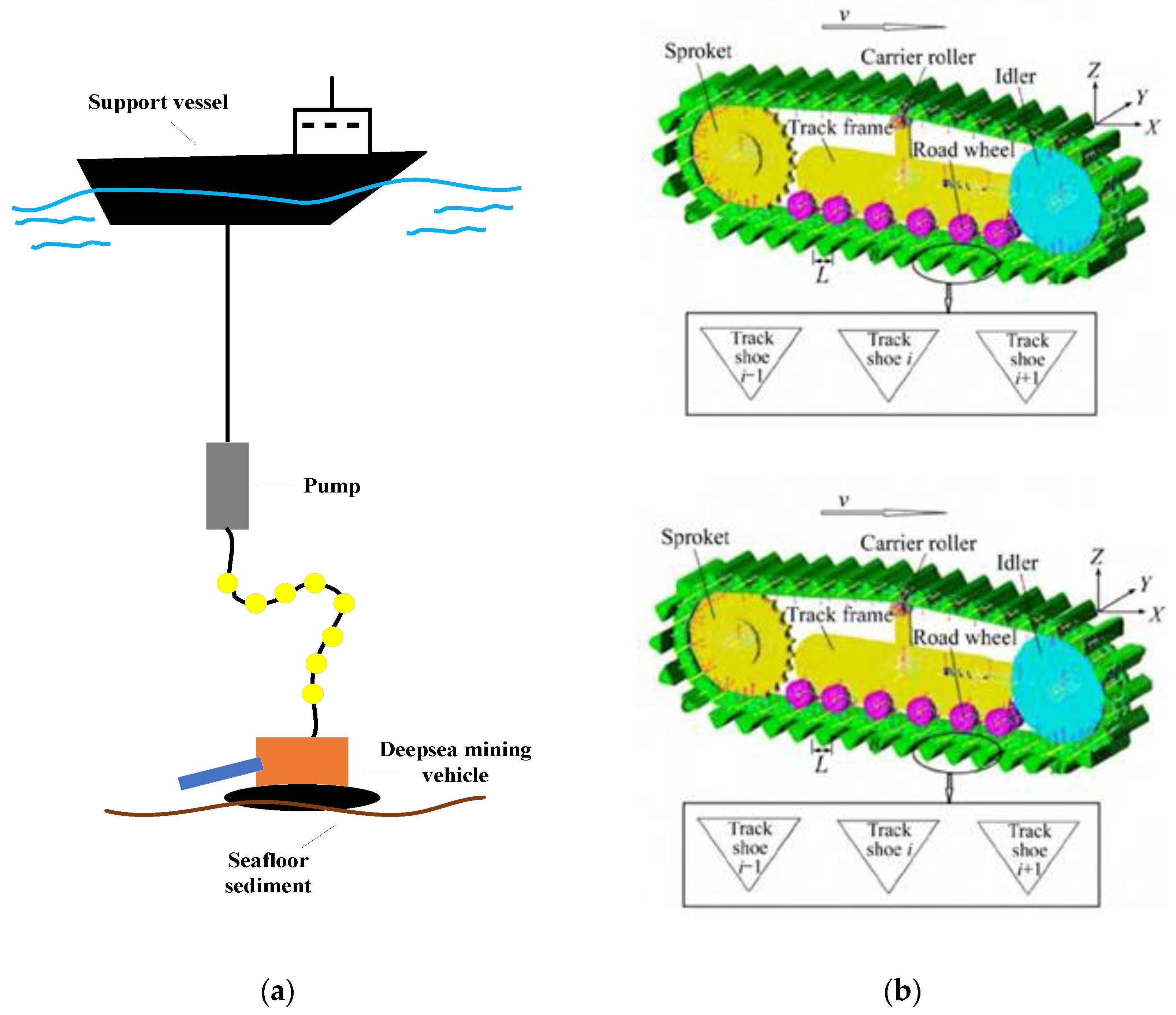
a) Schematic diagram of the deep-sea mining system, (b) the arrangement of the grouser and the track Reprinted from Ref. [3].
Jmse 10 01680 g001
Figure 2. Continuum deformation using (a) Lagrangian and (b) Eulerian methods.
Jmse 10 01680 g002
Figure 3. 
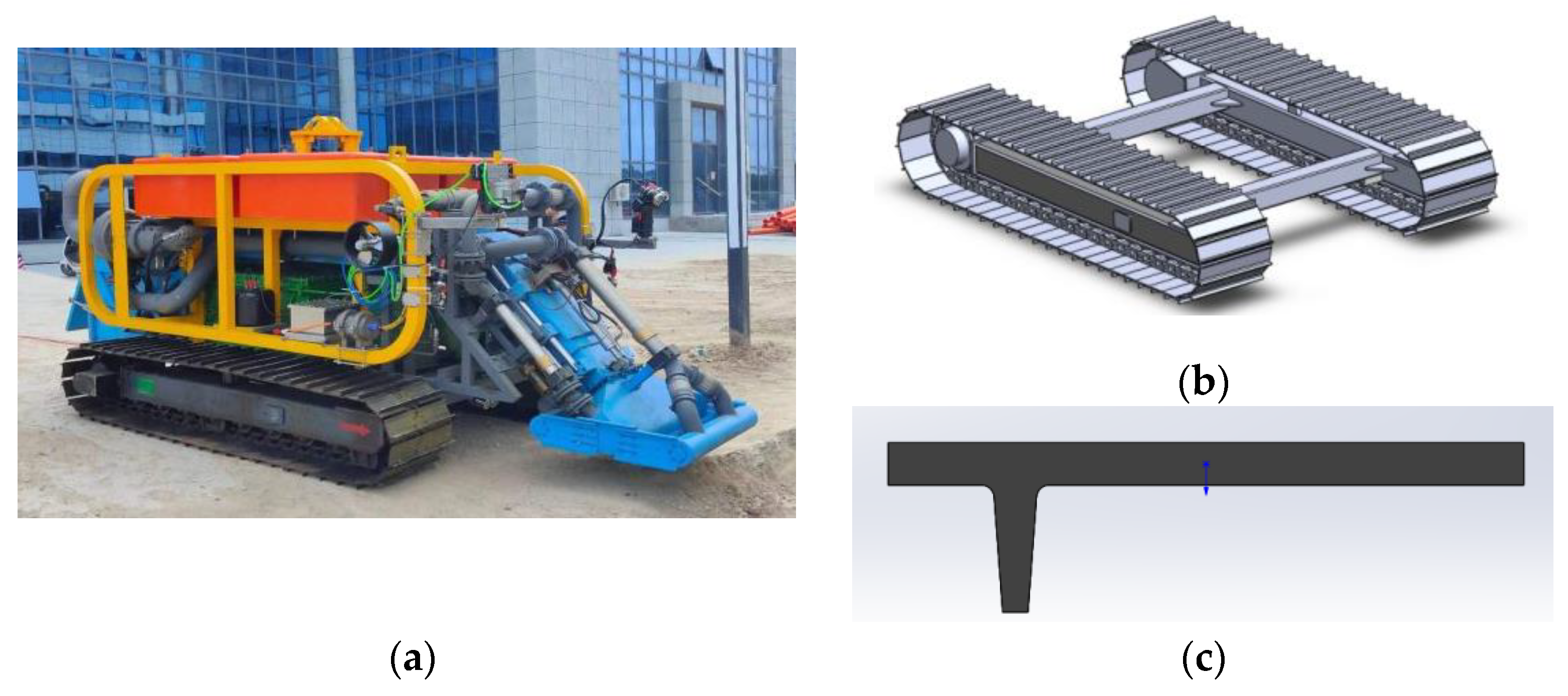
Structural details of “Pioneer-I” DSMV. (a) DSMV model, (b) Track mechanism, (c) Track plate model.
Jmse 10 01680 g003
Figure 4. Box sampler and retrieved soil samples. (a) Box sampler, (b) In situ sample, (c) Seafloor soil, (d) Field sampling.
Jmse 10 01680 g004
Figure 5. Laboratory test photos: (a) penetration resistance, (b) shear strength, (c) direct shear tests, (d) consolidation test.
Jmse 10 01680 g005
Figure 6. Overview of the numerical model of the track plate and the soil.
Jmse 10 01680 g006
Figure 7. Simulation results of geostatic stress balance. (a) The soil stress distribution, (b) the soil vertical displacement distribution.
Jmse 10 01680 g007
Figure 8. Three mesh seeds layout distribution.
Jmse 10 01680 g008
Figure 9. Sensitivity analysis results of each mesh seed. (a) Zone-1, (b) Zone-2, (c) Zone-3.
Jmse 10 01680 g009
Figure 10. Overall track plate-soil simulation model. (a) Overall model, (b) partial view of track plate, (c) side view of track plate.
Jmse 10 01680 g010
Figure 11. 
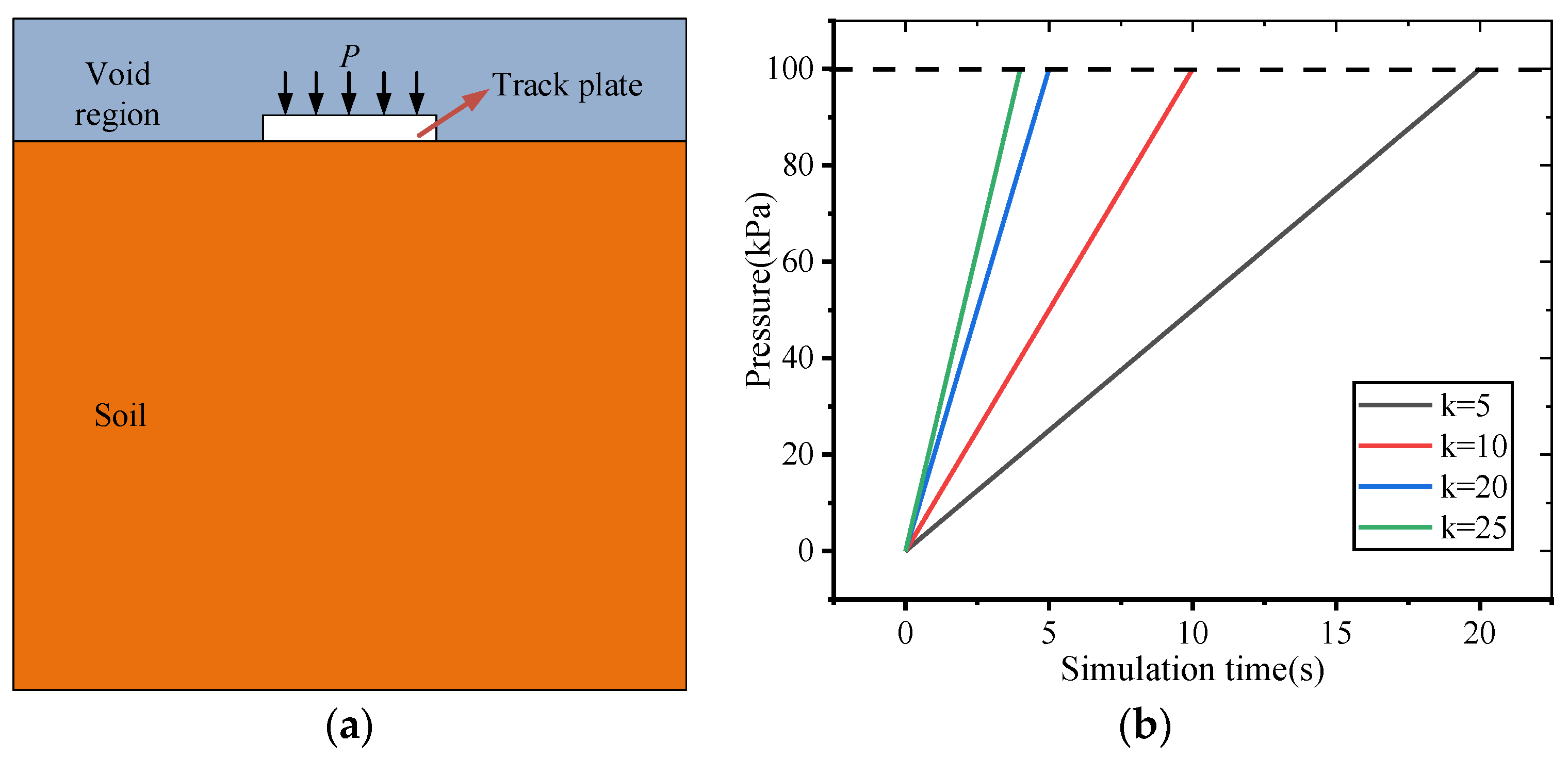
(a) Schematic diagram of numerical simulation and (b) the curve of pressure loading with time.
Jmse 10 01680 g011
Figure 12. (a) Pressure-sinkage curve and (b) the maximum displacement variation curve with k.
Jmse 10 01680 g012
Figure 13. Comparison between the numerical simulation (a) Simulation results, and the plate sinkage test, (b) test results [18].
Jmse 10 01680 g013
Figure 14. (a) Schematic diagram of numerical simulation and (b) curve of different velocities.
Jmse 10 01680 g014
Figure 15. Variation curves of resistance with displacement at different velocities.
Jmse 10 01680 g015
Figure 16. Schematic diagram of the track plate L and B.
Jmse 10 01680 g016
Figure 17. (a) Pressure-sinkage curves and (b) maximum sinkage under different conditions at 100 kPa case.
Jmse 10 01680 g017
Figure 18. (a) Comparison between pressure and S/B and (b) Maximum S/B comparison under different L/B ratios at 100 kPa case.
Jmse 10 01680 g018
Figure 19. Schematic diagram of the rectangle plate and the circle plate.
Jmse 10 01680 g019
Figure 20. (a) Comparison of maximum displacements under different L/B ratios and (b) pressure-sinkage curves when L/B = 6 and 8.
Jmse 10 01680 g020
Figure 21. Pressure-sinkage curves of different circular plate diameters.
Jmse 10 01680 g021
Figure 22. (a) Pressure-sinkage curves of different circular plate diameters and (b) maximum sinkage comparison at 100 kPa case.
Jmse 10 01680 g022
Figure 23. (a) Pressure-sinkage curves and (b) maximum sinkage at different grousers at 100 kPa case.
Jmse 10 01680 g023
Figure 24. Pressure-sinkage curves of different grouser shapes.
Jmse 10 01680 g024
Figure 25. (a) Pressure-sinkage curves of different soil height and (b) maximum sinkage comparison at 100 kPa case.
Jmse 10 01680 g025
Figure 26. (a) Pressure-sinkage curves of different IFA and (b) maximum sinkage comparison at 100 kPa case.
Jmse 10 01680 g026
Figure 27. (a) Pressure-sinkage curves of different cohesion and (b) maximum sinkage comparison at 100 kPa case.
Jmse 10 01680 g027
Figure 28. (a) Pressure-sinkage curves of different modulus of elasticity and (b) maximum sinkage comparison at 100 kPa case.
Jmse 10 01680 g028
Figure 29. Physical and mechanical parameters change curve with depth. (a) Density, (b) IFA, (c) cohesion.
Jmse 10 01680 g029
Figure 30. The pressure-sinkage curves of different physical and mechanical properties with soil depth.
Jmse 10 01680 g030
Figure 31. Comparison of the flow chart between (a) Lagrangian and (b) Eulerian heterogeneous soil establishment.
Jmse 10 01680 g031
Figure 32. (a) The soil material distribution and (b) the density distribution.
Jmse 10 01680 g032
Figure 33. (a) Pressure-sinkage curves under different conditions and (b) curve under the heterogeneous soil conditions.
Jmse 10 01680 g033
Figure 34. Soil stress contours of three soil types.
Jmse 10 01680 g034
Table 1. Summary of pressure–sinkage models in the literature.
YearReferencePressure–Sinkage ModelClassification
1885Boussinesq Reprinted from Ref. [5] p = 2 C f E 1 v 2 z B Analytical models
1944Terzaghi Reprinted from Ref. [6] p = c N c λ c + B 2 γ N γ λ γ + γ N q λ q z
1987Ageikin Reprinted from Refs. [7,8] p = 2 E B H z 2 E z + π B H A 0 B J Q
1913Bernstein Reprinted from Ref. [9] p = k z n Empirical
models
1959Saakyan Reprinted from Ref. [10] p = k ( z D ) n
1963Tsytovich Reprinted from Ref. [11] p = z T A
1965E. Hegedus Reprinted from Ref. [12] p = γ l A 1 m B ( z S ) 1 m
1967Onafeko and Reece Reprinted from Ref. [13] p = ( k 1 + k 2 b ) ( z b ) n
1969Bekker Reprinted from Ref. [14] p = ( k c b + k φ ) z n
1982Youssef and Ali Reprinted from Ref. [15] p = ( k 1 + α b k 2 ) ( β ) n ( z b ) n
1982Wong et al.Reprinted from Ref. [16] P = k p z + 4 m m z 2 D h
1985M. A. Sargana et al.Reprinted from Ref. [17] p = ( k c b + k φ ) z n + ( η b + η ) z m ( v ¯ ) α
2006Gotteland and BenoitReprinted from Ref. [18] p = ( C m B m + S m B 1 m z ) ( 1 exp { S 0 C m z B 1 m } )
2010Lyasko Reprinted from Ref. [19] p = 1 D 1 B i + D 2 E z ω B ζ
Table 2. DSMV and track structural parameters.
DSMV Structural ParametersTrack Structural Parameters
Length × width × height5 m × 2.5 m × 2.1 mLength × width × height3.26 m × 2.5 m × 2.1 m
Vehicle weightIn air ≈ 9.5 t;
In water ≈ 6 t
Track width0.6 m
Ground specific pressure15 kPaTrack ground area4 m2
Velocity0.5 m/sChassis bearing capacity8 t
Maximum climbing capability15°Track spacing1.3 m
Working water depth3000 mChassis weight2 t
Table 3. Physical properties of the seafloor soil.
Depth (cm)Moisture Content (%)Wet Density
(g/cm3)
Dry Density
(g/cm3)
Natural Porosity RatioSaturationIL
0–15153.21.260.504.4260.9356.05
15–30125.31.340.593.5400.9564.73
30–4596.41.440.732.6830.973.40
Table 4. The seafloor composition.
Depth (cm)Sand (%)Silt (%)Clay (%)
0–157.78273.16319.054
15–307.41169.89122.698
30–437.88969.10323.008
Table 5. Main mechanical properties of soil.
PropertyMeasurement Data
Shear strength2–5 kPa
Compression modulus1.5–1.7 MPa
Penetration resistance20–110 kPa
CohesionAverage 9 kPa
Internal friction angle2.2–5°
Table 6. Physical and mechanical characteristics of the soil model.
DensityCohesionInternal Friction AngleFriction
Coefficient
Elastic
Modulus
Poisson’s Ratio
1400 kg/m35 kPa0.32.5 MPa0.49
Table 7. Mesh sensitivity parameter setting.
Mesh Zone NumberMesh Seed Values (m)
Zone-10.020.030.040.050.1
Zone-20.020.030.040.050.1
Zone-30.020.030.040.050.1
Table 8. The mesh seed value.
Zone-1Zone-2Zone-3
0.03 m0.1 m0.03 m
Table 9. Comparison of numerical calculation and prediction formula for maximum displacement of L/B = 5 and 10.
L/B Ratio510
Equation calculationMaximum sinkage 0.343 mMaximum sinkage 0.138 m
Numerical calculationMaximum sinkage 0.35 mMaximum sinkage 0.13 m
The percentage error2.04%5.8%
Table 10. Different grouser types and numbers setting.
Grouser TypeThree-Dimensional StructureGrouser TypeThree-Dimensional Structure
Tri-shaped Jmse 10 01680 i001Parabola-shaped Jmse 10 01680 i002
Single T-shaped Jmse 10 01680 i003Double T-shaped Jmse 10 01680 i004
Triple T-shaped Jmse 10 01680 i005
Table 11. Different grouser types and value setting.
The Study ParameterValue
Internal friction angle (°)351015202530
Cohesion (kPa)510152030--
Elastic modulus (Mpa)2070120180240--
Table 12. Soil parameters as a function of depth.
ProjectFunctionFunctional Form
Density-1 ρ = ( 1200 2228 ) / ( 1 + ( d / 0.23 ) 1.64 ) + 2228 ( ρ , Φ , c ) = ( A 1 A 2 ) / ( 1 + ( d / x 0 ) p ) + A 2
Density-2 ρ = ( 1200 2670 ) / ( 1 + ( d / 0.98 ) 1.06 ) + 2670
IFA-1 Φ = ( 3 25.5 ) / ( 1 + ( d / 0.23 ) 1.76 ) + 25.5
IFA-2 Φ = ( 2.98 30.5 ) / ( 1 + ( d / 0.66 ) 1.24 ) + 30.5
Cohesion-1 c = ( 9 31.88 ) / ( 1 + ( d / 0.281 ) 1.28 ) + 31.88
Cohesion-2 c = ( 9 38.46 ) / ( 1 + ( d / 0.78 ) 1.25 ) + 38.46
Density-3 ρ = 1200 + 500 d ( ρ , φ , c ) = k d + B
IFA-3 Φ = 3 + 11 d
Cohesion-3 c = 9 + 10.5 d
Density-4 ρ = 100 e ( d / 0.834 ) + 1100 ( ρ , Φ , c ) = A 1 e ( d / t 1 ) + y 0
Density-5 ρ = 1.58 e ( d / 0.31 ) + 1199
IFA-4 Φ = 2.26 e ( d / 0.84 ) + 0.74
IFA-5 Φ = 0.0225 e ( d / 0.29 ) + 3
Cohesion-4 c = 2.26 e ( d / 0.84 ) + 0.74
Cohesion-5 c = 0.225 e ( d / 0.29 ) + 3
Table 13. Working condition name and corresponding physical and mechanical parameters label.
ProjectDensityIFACohesion
Nolinear-1Density-1IFA-1Cohesion-1
Nolinear-2Density-2IFA-2Cohesion-2
linearDensity-3IFA-3Cohesion-3
Nolinear-3Density-4IFA-4Cohesion-4
Nolinear-4Density-5IFA-5Cohesion-5
Publisher’s Note: MDPI stays neutral with regard to jurisdictional claims in published maps and institutional affiliations.

