Numerical Simulation Research on the Anchor Last Deployment of Marine Submersible Buoy System Based on VOF Method

Abstract

Marine submersible buoy systems are widely-used equipment for ocean resource development. The marine submersible buoy system studied in this paper consists of the submersible buoy, the battery compartment, the anchor block, the mooring line, and the power supply cable. To study the mechanical behavior and obtain the speed variation of each component during the anchor last deployment, this paper establishes the free surface computational fluid dynamics model of marine submersible buoy systems based on the VOF method. This model includes the incompressible Navier–Stokes equations, the Renormalization-Group turbulence model, and the fractional areas/volume obstacle representation method. The free fluid surface is tracked using the VOF method. The lumped mass method is used to simulate the mooring line and power supply cable. The results showed that the tension forces increase when the mooring lines were straightened. Subsequently, the tension forces gradually decrease with oscillations. After the anchor block sinks to the sea floor, the positive buoyancy of the battery compartment and the buoy will cause large tension on the mooring line and power supply cable.

1. Introduction

With the deepening of seabed scientific research and comprehensive utilization of ocean resources, the demand for underwater exploration is increasing. The marine submersible buoy system is widely used for ocean resource development. It is highly efficient, convenient, has a low energy cost, and is recyclable. It plays an increasingly important role in the exploitation of marine resources, information acquisition, and underwater target characteristics [1]. Unlike single-point moorings buoys and CALM (catenary anchor leg moorings) buoys, the submersible buoy is closer to the seabed. Thus, its advantage lies in being more suitable for seabed environment exploration.

The marine submersible system consists of a submersible buoy, a battery compartment, an anchor block, a mooring line, and a power supply cable. As shown in Figure 1, the anchor block is connected to the battery compartment through the mooring line, and the battery compartment is connected to the submersible buoy through the power supply cable. The anchor block is made of reinforced concrete, and its density is 3.5 g/cm³, which is greater than the density of water. The density of the submersible buoy and battery compartment is less than that of water.

Anchor last deployment is a typical deployment method for submersible buoy systems. As the name indicates, the anchor is the last component to be deployed. In the anchor last deployment of the submersible buoy system, the submersible buoy and battery compartment are first set down on the sea surface, and then the anchor block is thrown into the water from the deck of the ship. The anchor block will sink quickly after being thrown into the water. Eventually, the anchor will pull the battery compartment and the submersible down to the seabed. Due to the inertia of the anchor block, it will produce large impact tension on the mooring line and power supply cable when pulling the submersible buoy system down. In the process of deployment, the mooring line and power supply cable must not break or the deployment will fail. To study the mechanical behavior and obtain the velocity variation of each component during the anchor last deployment, this paper establishes the free surface computational fluid dynamics model of marine submersible buoy systems based on the VOF method.

The most significant tension force increase occurs at the moment when the mooring line and power supply cable are straightened. At the same time, the battery compartment and the submersible buoy are pulled into the water. The tension forces of the mooring lines and power supply cable are directly related to the water entry process of the battery compartment. This paper establishes the VOF computational fluid dynamics model for the deployment of a marine submersible buoy system to study the mechanical behavior of the mooring line and power supply cable.

Various investigations have been carried out on the mechanical behavior of submersible buoy systems and mooring systems. Hamilton et al. (2003) presented a comparison between numerical model predictions and actual measurements of the tension of an ocean observing system [2]. O.B. Augusto et al. (2003) explored a planning methodology for deep water anchor deployment in offshore platforms and floating production systems aiming at operational resource optimization [3]. J.I. Gobat et al. (2006) describe the numerical features of WHOI Cable, a computer program for analyzing the statics and dynamics of oceanographic cable structures [4]. Chang, Z.Y. et al. (2011) studied a single-point mooring buoy system that contains a surface buoy, cable segments with components, anchor, and so on, and is modeled by applying the multi-body dynamics method [5]. The motion equations are developed in discrete node description and fully Cartesian coordinates. Zheng Zhongqiang et al. (2012) used a numerical method to solve the ordinary differential equations and dynamics simulations achieved while the anchor is cast from onboard, then (2016) studies the deployment dynamics of submersible buoy systems with numerical and experimental methods [6,7]. Yang Yu et al. (2019) investigated the effect of liquid sloshing of inner tanks on the dynamic responses of an underwater soft yoke mooring system. Inner tanks with different filling levels were examined under different external wave loads in towing tank experiments [8]. Yang Q et al. (2019) carried out actual testing, hydrodynamic simulations, and acoustic simulations to solve the problem of vertical cable attitudes that affect the performance of the submarine system [9]. Wenxian Tang et al. (2019) used ANSYS to perform a numerical analysis to examine the performance of a mooring system in time and frequency domains [10]. Imanol Touzon et al. (2020) validate a numerical model of the HarshLab2.0 floating platform coupled with a non-linear lumped mass catenary mooring system in a small-scale experiment [11]. Srinivasan Chandrasekaran et al. (2021) carried out coupled dynamic analyses of a deep-water semi-submersible platform, in the south China sea region under postulated damage of the restraining system for both 10 and 100-years return period events [12]. Changqing Jiang et al. (2021) compared a numerical method that coupled a Reynolds-averaged Navier–Stokes solver with a quasi-static and a dynamic mooring model [13]. Ray-Yeng Yang et al. studied the dynamic responses of an oil tanker moored on a catenary anchor leg mooring (CALM) buoy. The operating conditions simulated included under the wave, wind, and current through numerical simulations [14]. Chiemela Victor Amaechi et al. (2022) carried out numerical studies on CALM buoy motion responses and the effect of buoy geometry cum skirt dimensions with its hydrodynamic waves-current interactions [15,16]. Atefeh Neisi et al. (2022) proposed two hybrid mooring systems to improve the performance of the dynamic motions of the floating platform [17].

Completed studies in the literature of the anchor last deployment of marine submersible buoy system were usually based on the multi-body dynamics method, which is a simple and effective method to get the tension force on cables [5,6,7]. However, as shown in Figure 2, the huge tension force on cables usually occurs at the moment when the buoy is dragged into the water, and the tension force on the cables is highly concerning due to the bouy’s entry into the water. In addition, the multi-body dynamics method cannot track the wake of the block, which may reduce water resistance to the bouy. In this paper, we propose a computation fluid dynamic model of the marine submersible buoy system to study the anchor last deployment process, using the VOF method to track the free surface. Simulations are then conducted to investigate the anchor last deployment process, from the initial water entry process until the anchor block sinks to the seabed. Results show that the tension increases with the weight of the anchor block. The significant tension force increase occurs at the moment when the mooring line is straightened.

2. Numerical Methods

2.1. Free Surface Model

Based on the fractional areas/volume obstacle representation method [18], the three-dimensional incompressible Navier–Stokes equations in the cartesian coordinate system are established as follows:

$$\left\{\begin{array}{l}\frac{\partial u}{\partial t}+\frac{1}{V_F}\left(u{A}_x\frac{\partial u}{\partial x}+v{A}_y\frac{\partial u}{\partial y}+w{A}_z\frac{\partial u}{\partial z}\right)=-\frac{1}{\rho }\frac{\partial p}{\partial x}+G_x+f_x\hfill \\ \frac{\partial v}{\partial t}+\frac{1}{V_F}\left(u{A}_x\frac{\partial v}{\partial x}+v{A}_y\frac{\partial v}{\partial y}+w{A}_z\frac{\partial v}{\partial z}\right)=-\frac{1}{\rho }\frac{\partial p}{\partial y}+G_y+f_y\hfill \\ \frac{\partial w}{\partial t}+\frac{1}{V_F}\left(u{A}_x\frac{\partial w}{\partial x}+v{A}_y\frac{\partial w}{\partial y}+w{A}_z\frac{\partial w}{\partial z}\right)=-\frac{1}{\rho }\frac{\partial p}{\partial z}+G_z+f_z\hfill \end{array}\right.$$

(1)

$$\left\{\begin{array}{l}{f}_x=-\frac{1}{\rho V_F}\left[\frac{\partial }{\partial x}\left(A_x{\tau }_{xx}\right)+\frac{\partial }{\partial y}\left(A_y{\tau }_{xy}\right)+\frac{\partial }{\partial z}\left(A_z{\tau }_{xz}\right)\right]\hfill \\ f_y=-\frac{1}{\rho V_F}\left[\frac{\partial }{\partial x}\left(A_x{\tau }_{xy}\right)+\frac{\partial }{\partial y}\left(A_y{\tau }_{yy}\right)+\frac{\partial }{\partial z}\left(A_z{\tau }_{yz}\right)\right]\hfill \\ f_z=-\frac{1}{\rho V_F}\left[\frac{\partial }{\partial x}\left(A_x{\tau }_{xz}\right)+\frac{\partial }{\partial y}\left(A_y{\tau }_{yz}\right)+\frac{\partial }{\partial z}\left(A_z{\tau }_{zz}\right)\right]\hfill \end{array}\right.$$

(2)

$$\left\{\begin{array}{l}{\tau }_{xx}=-2\mu \left[\frac{\partial u}{\partial x}-\frac{1}{3}\left(\frac{\partial u}{\partial x}+\frac{\partial v}{\partial y}+\frac{\partial w}{\partial z}\right)\right]\hfill \\ {\tau }_{xy}=-\mu \left(\frac{\partial v}{\partial x}+\frac{\partial u}{\partial y}\right)\hfill \\ {\tau }_{yy}=-2\mu \left[\frac{\partial v}{\partial y}-\frac{1}{3}\left(\frac{\partial u}{\partial x}+\frac{\partial v}{\partial y}+\frac{\partial w}{\partial z}\right)\right]\hfill \\ {\tau }_{xy}=-\mu \left(\frac{\partial u}{\partial z}+\frac{\partial w}{\partial x}\right)\hfill \\ {\tau }_{zz}=-2\mu \left[\frac{\partial w}{\partial z}-\frac{1}{3}\left(\frac{\partial u}{\partial x}+\frac{\partial v}{\partial y}+\frac{\partial w}{\partial z}\right)\right]\hfill \\ {\tau }_{yz}=-\mu \left(\frac{\partial v}{\partial z}+\frac{\partial w}{\partial y}\right)\hfill \end{array}\right.$$

(3)

where ρ is the fluid density, and u, v, and w are the fractional quantities of the surface product of the fluid velocity above x, y, and z directions, respectively. $A_x$, $A_y$ and $A_z$ are the fluid in the x, y, and z directions, respectively, $V_F$ is the volume fraction of the fluid; P is fluid pressure, $G_x$, $G_y$ and $G_z$ are gravitational acceleration, and $f_x$, $f_y$ and $f_z$ are the accelerations of viscous forces.

The viscosity of the fluid is considered based on RANS equations [19,20]. Compared with the standard k-ε model, it is more suitable to describe the flow in the region with strong shear in the deployment. The RNG model uses equations similar to the equations for the k-ε model. However, equation constants that are found empirically in the standard k-ε model are derived explicitly in the RNG model. The equation k of turbulent kinetic energy is

$$\frac{\partial }{\partial t}\left(\rho k\right)+\frac{\partial }{\partial x_i}\left(\rho k{u}_i\right)=\frac{\partial }{\partial x_j}\left[{\sigma }_k\left(\mu +{\mu }_t\right)\frac{\partial k}{\partial x_j}\right]+G_k-\rho \epsilon$$

(4)

where $u_i$ and $u_j$ are velocity components in the direction of $x_i$ and $x_j$, $\mu$ is fluid viscosity, ${\mu }_t$ is dynamic viscosity, $G_k$ is the generation term of turbulent kinetic energy k caused by average velocity gradient, constant coefficient ${\sigma }_k$ = 1.39.

The turbulent dissipation rate $\epsilon$ equation is

$$\frac{\partial }{\partial t}\left(\rho k\right)+\frac{\partial }{\partial x_i}\left(\rho k{u}_i\right)=\frac{\partial }{\partial x_j}\left[{\sigma }_k\left(\mu +{\mu }_t\right)\frac{\partial k}{\partial x_j}\right]+G_k-\rho \epsilon +C_{1\epsilon }^{*}\frac{\epsilon }{k}{G}_k-C_{2\epsilon }\rho \frac{{\epsilon }^2}{k}$$

(5)

where equation coefficient $C_{1\epsilon }^{*}$, Constant coefficient $C_{2\epsilon }$ and ${\sigma }_{\epsilon }$ are given by

$$\left\{\begin{array}{l}{C}_{1\epsilon }^{*}=C_{1\epsilon }-\frac{\eta \left(1-\eta /{\eta }_0\right)}{1+\beta {\eta }^3},\eta ={\left(2E_{ij}\cdot E_{ij}\right)}^{1/2}\frac{k}{\epsilon }\hfill \\ E_{ij}=\frac{1}{2}\left(\frac{\partial u_i}{\partial x_j}+\frac{\partial u_j}{\partial x_i}\right),{\sigma }_{\epsilon }=1.39\hfill \\ C_{1\epsilon }=1.42,C_{2\epsilon }=1.68\hfill \\ {\eta }_0=4.377,\beta =0.012\hfill \end{array}\right.$$

(6)

The free fluid surface was solved by the fluid volume function (VOF) proposed by Hirt et al. [21]. The free liquid surface boundary is determined by calculating the fluid and mesh volume ratio function F (x, y, z, t) in the grid element.

$$\frac{\partial F}{\partial t}+\frac{1}{V_F}\left[\frac{\partial }{\partial x}\left(F{A}_{x}u\right)+\frac{\partial }{\partial y}\left(F{A}_{y}v\right)+\frac{\partial }{\partial z}\left(F{A}_{z}w\right)\right]=0$$

(7)

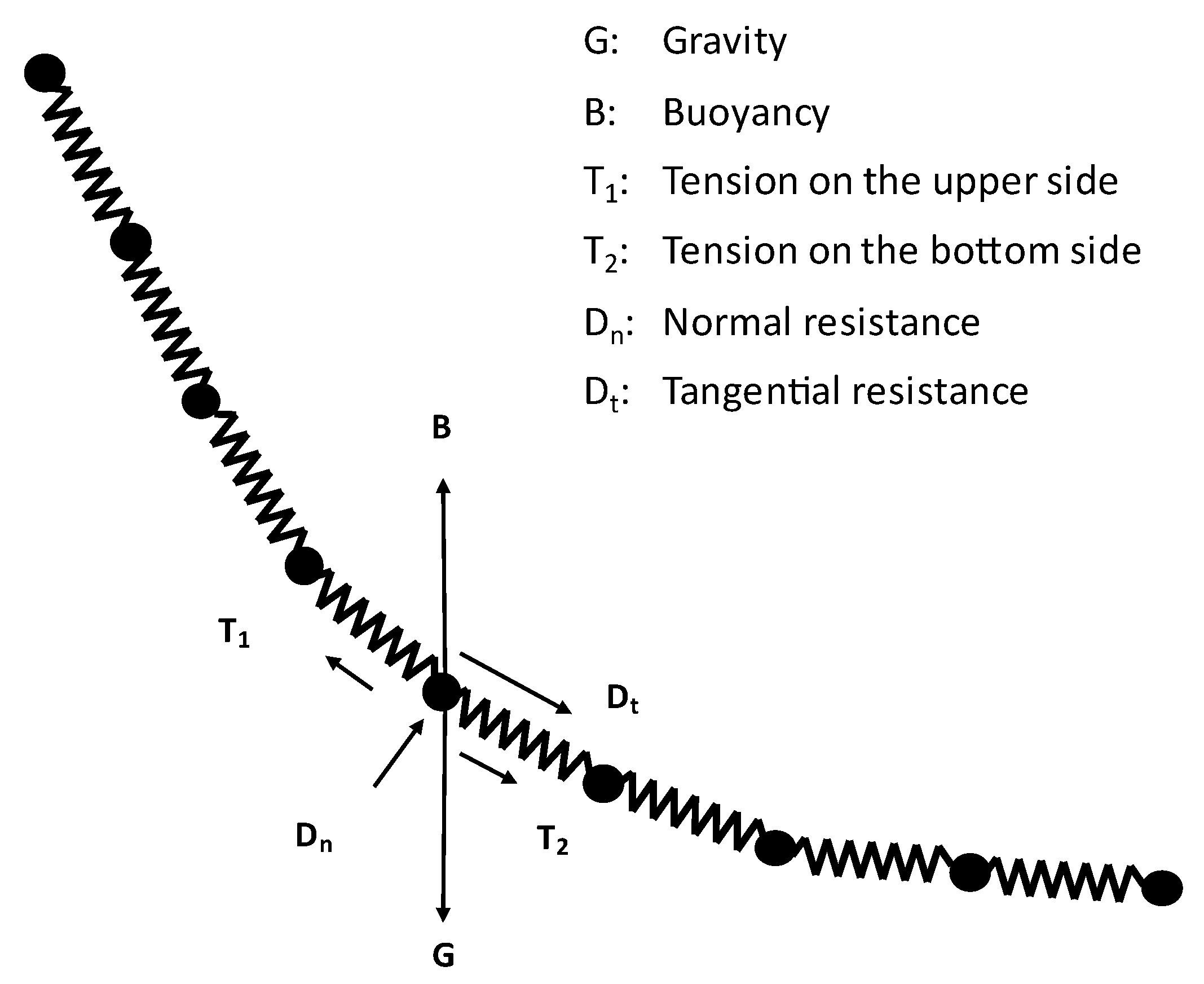
2.2. Mooring Line and Power Supply Cable Model

The power supply cable and the mooring line are simulated by lumped mass method, which is widely used in the simulation of the mooring line [22]. This method divides the cable into several segments for calculation. It is assumed that each segment of the cable is a cylinder with a uniform diameter and uniform material distribution. The kinetic equation of the piecewise motion is

$$m_p\frac{d{V}_p}{dt}=G+B+T_1+T_2+D_n+D_t$$

(8)

where G is gravity, B is buoyancy, $m_p$ is segment mass, $V_p$ is the velocity at the center of segment mass, $T_1$ and $T_2$ are tension at both ends of the segment, respectively, $D_n$ and $D_t$ are normal and tangential resistance of the segment, respectively.

$$\left\{\begin{array}{c}{D}_n=-C_{D,n}{\rho }_f{A}_n{v}_{r,n}\left|v_r\right|\\ D_t=-C_{D,t}{\rho }_f{A}_t{v}_{r,t}\left|v_r\right|\end{array}\right.$$

(9)

where, $C_{D,n}$ and $C_{D,t}$ are tangential and normal drag coefficients of segments, respectively, $v_r$ is the relative velocity between the segment and the surrounding fluid, $v_{r,n}$ and $v_{r,t}$ are the tangential and normal components of $v_r$ in the segment, respectively, ${\rho }_f$ is the fluid density. $A_n$ is the cross-sectional area of the segment, $A_t$ is the longitudinal area of the segment. Figure 3 illustrates the lumped mass method and the forces on a segment.

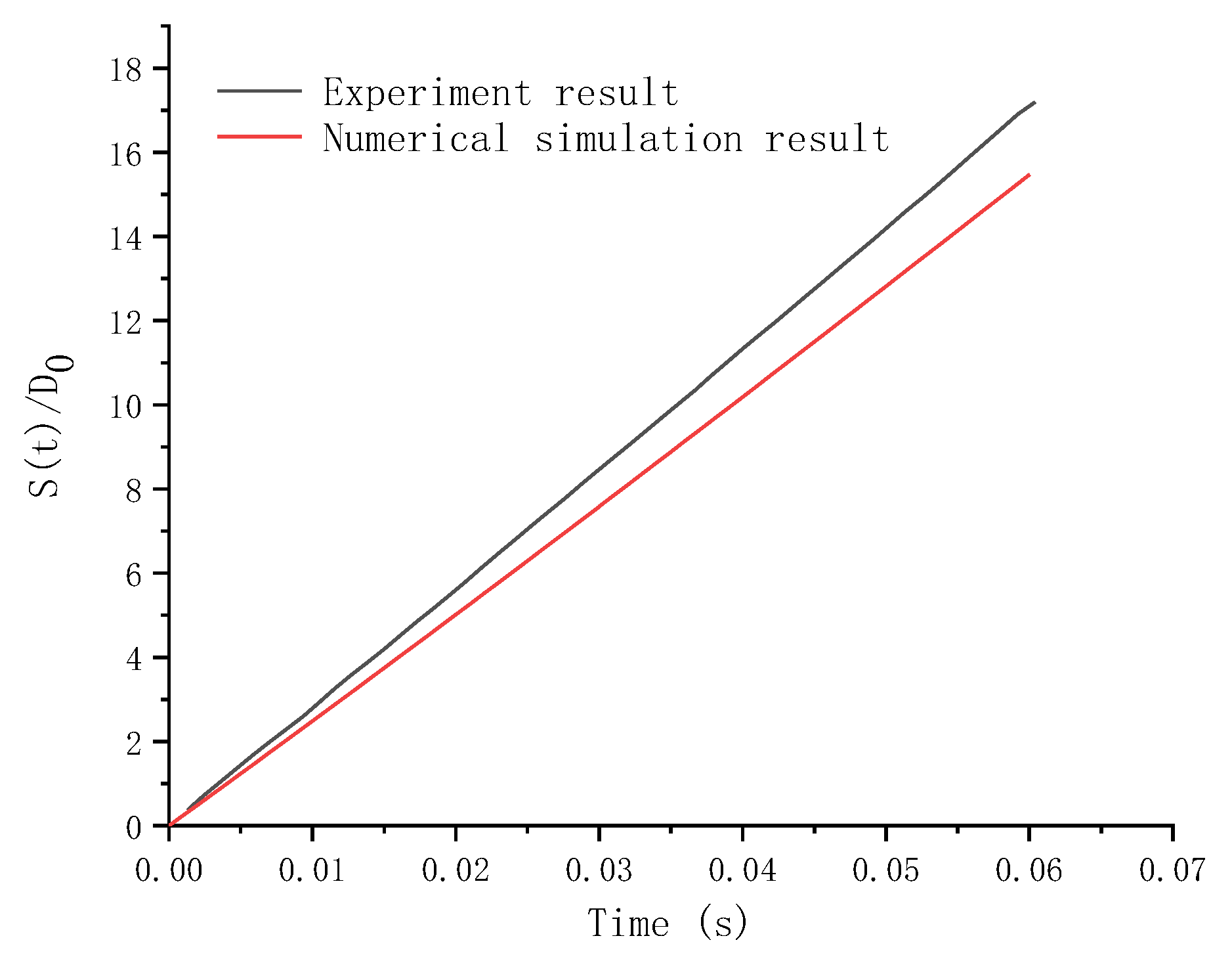
3. Numerical Method Verification

According to the free fluid surface model above, the water entry process of a 140 degrees cone angle steel cylinder was calculated and compared with the experiment conducted by He Chuntao to verify the accuracy of the VOF model [23]. Figure 4 illustrates the flow regime comparison between the experiment and simulation. Figure 5 illustrates the ratio of displacement to the diameter as a function of time between the experiment and simulation. It can be seen from the results that the VOF model in this paper can closelysimulate the flow regime of objects entering the water from the free fluid surface.

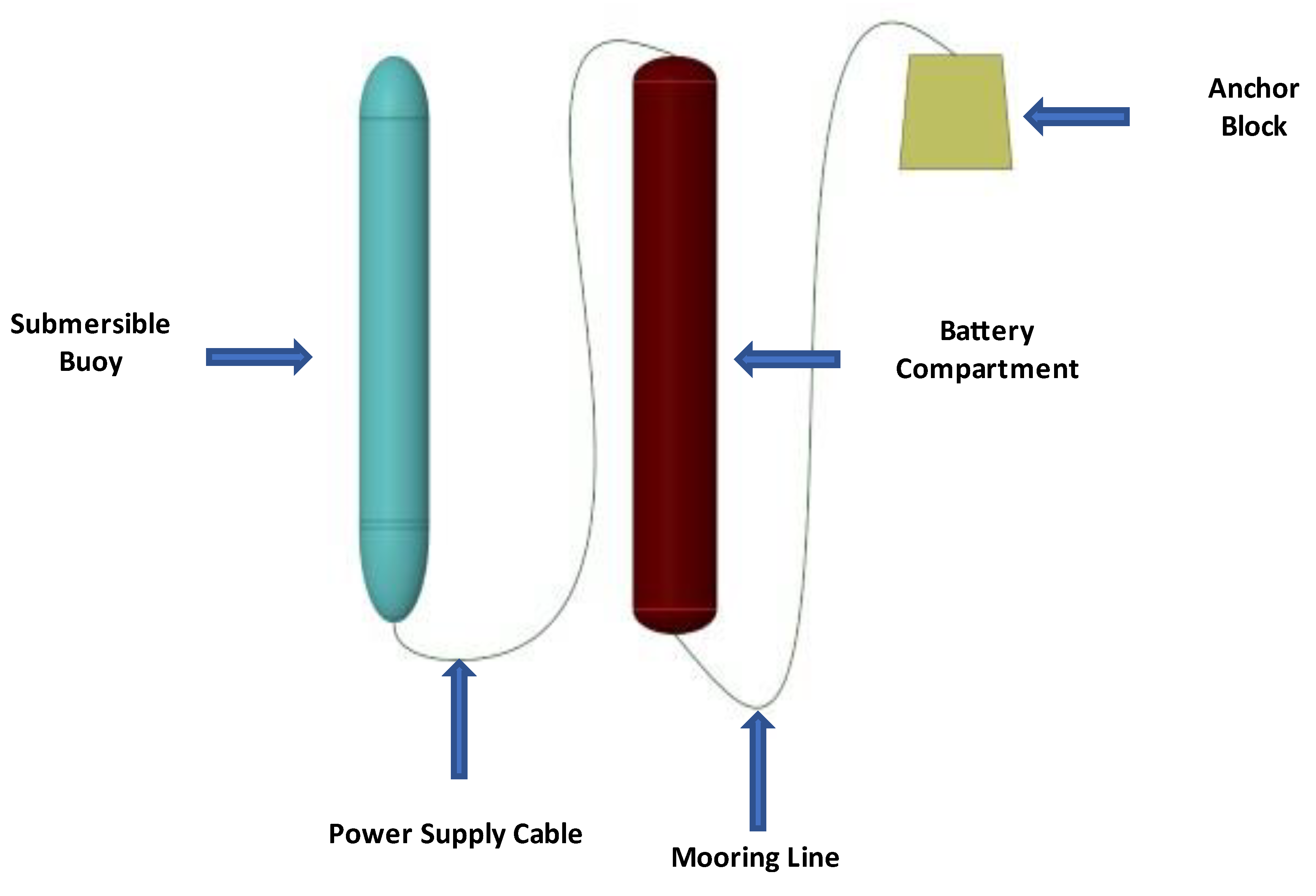
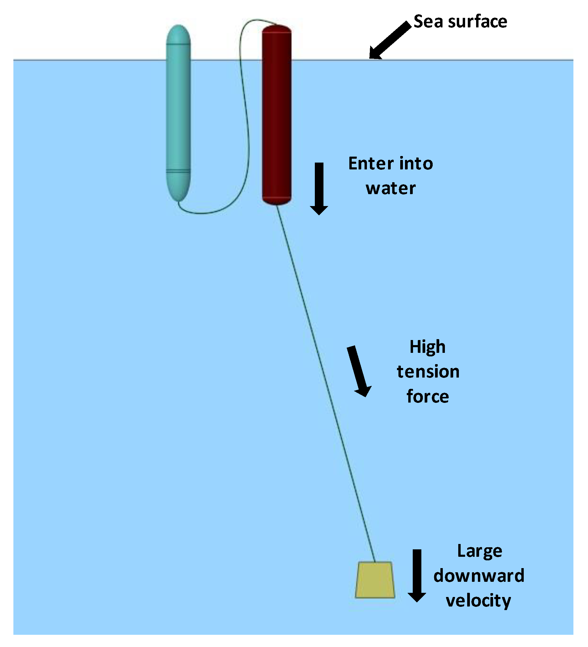
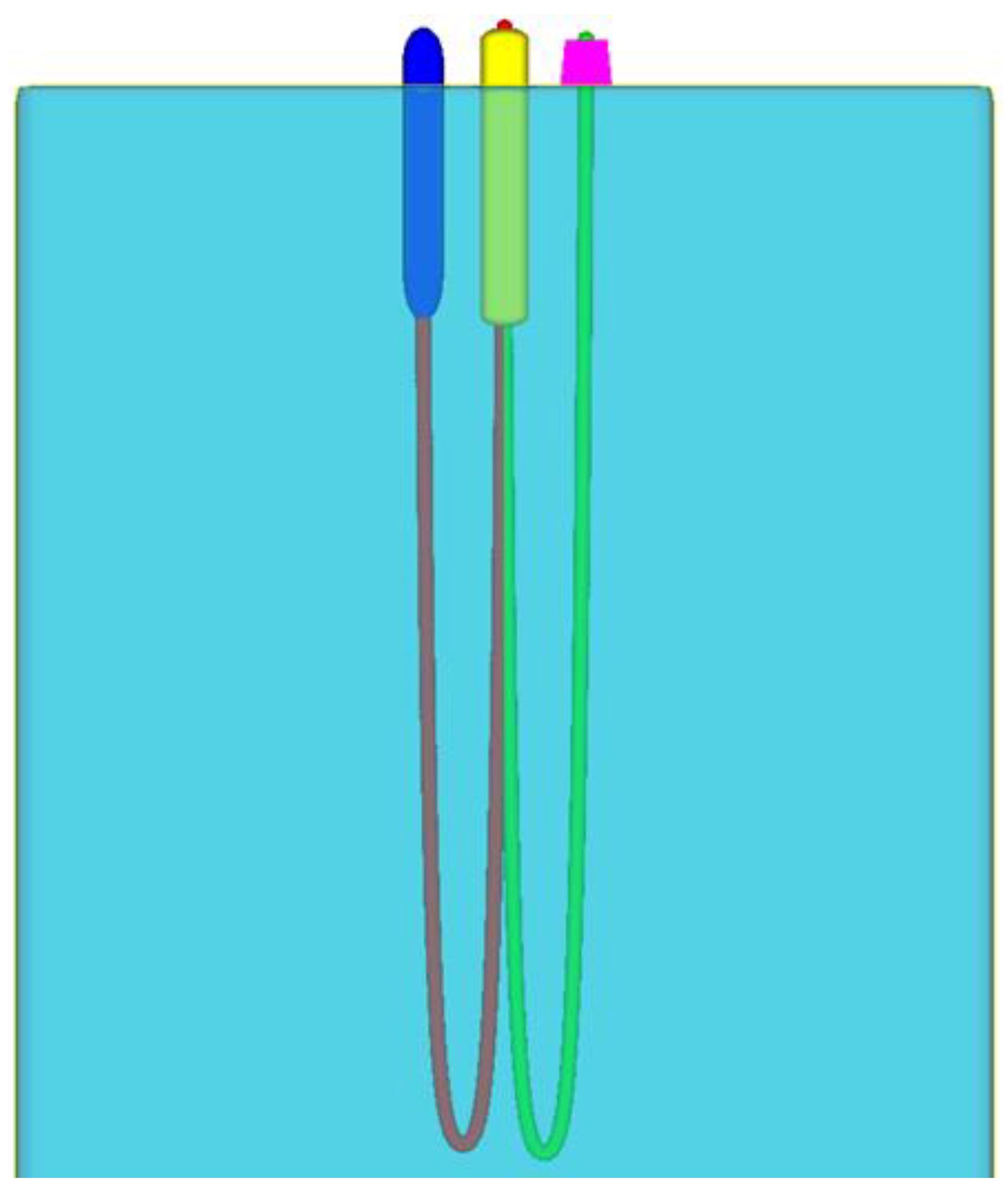
4. Calculation Model

The computation domain size in our next simulations is 6 m × 3 m × 51 m. Under the initial conditions, the submersible buoy and battery compartment are floating on the water’s surface as illustrated in Figure 6. The anchor block has an initial velocity of 7.67 m/s. This velocity corresponds to the anchor block falling from the 3 m high ship deck to the water’s surface. The length of the mooring line and power supply cable is 12 m. The deployment under the different underwater net weights of the anchor block is calculated. The underwater net weight of the anchor block was calculated at 60 kg, 80 kg, 100 kg, and 120 kg, respectively. The calculation time is from 0 s to 25 s to study the whole deployment process until the anchor block sinks to the sea bed.

The boundary condition of the fluid dynamic model is illustrated in Figure 7. The top surface uses a specified pressure boundary condition, which specifies the pressure at the boundary. The pressure is standard atmosphere pressure atm. The bottom surface uses the wall boundary condition, which applies the no-slip condition at the boundary as well as the zero velocity condition normal to the boundary. Besides, the wall boundary can collide with the anchor block. It can simulate the anchor block sinking to the seabed. The other four surfaces use a symmetry boundary condition, which applies a zero-gradient condition at the boundary as well as a zero velocity condition normal to the boundary.

Table 1. Parameters of components in submersible buoy systems.

Component	Gravity	Net Buoyancy
Submersible buoy	65 kg	152.88 N
Battery compartment	100 kg	257.74 N

shows the parameters of components in submersible buoy systems.

Table 2. Parameters of cables in submersible buoy systems.

Cable	Length	Modulus of Elasticity
Mooring line	12 m	25,000 N
Power supply cable	12 m	50,000 N

shows the parameters of cables in submersible buoy systems.

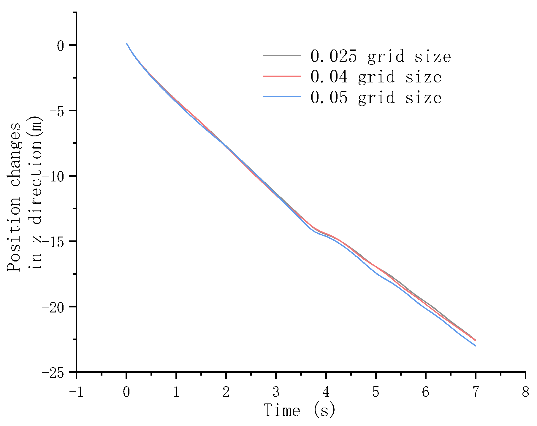
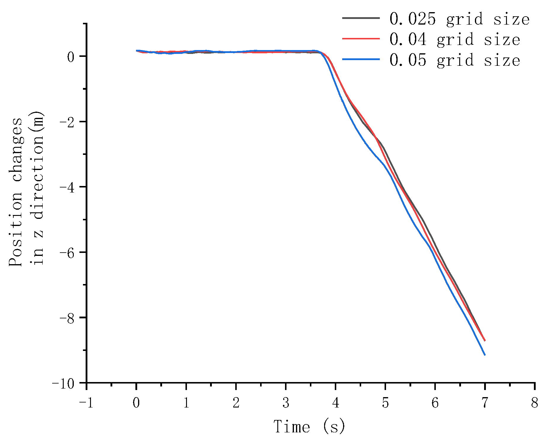
5. Grid Independence Verification

The grid independence was verified by using the 80 kg net weight anchor block, and mesh sizes at the center of the computational domain of 0.05 m, 0.04 m, and 0.025 m are compared. The number of grids is, respectively, 2.62 × 10⁶, 3.23 × 10⁶, and 7.15 × 10⁶. The calculation time is from 0 s to 7 s. The displacement changes of the anchor block and battery compartment in the z direction under three grid sizes were compared.

It can be seen from Figure 8 and Figure 9 that there is little difference between 0.04 m grid size and 0.025 m grid size, and 0.04 m was selected as the size of the computational grid.

6. Calculation Results and Analysis

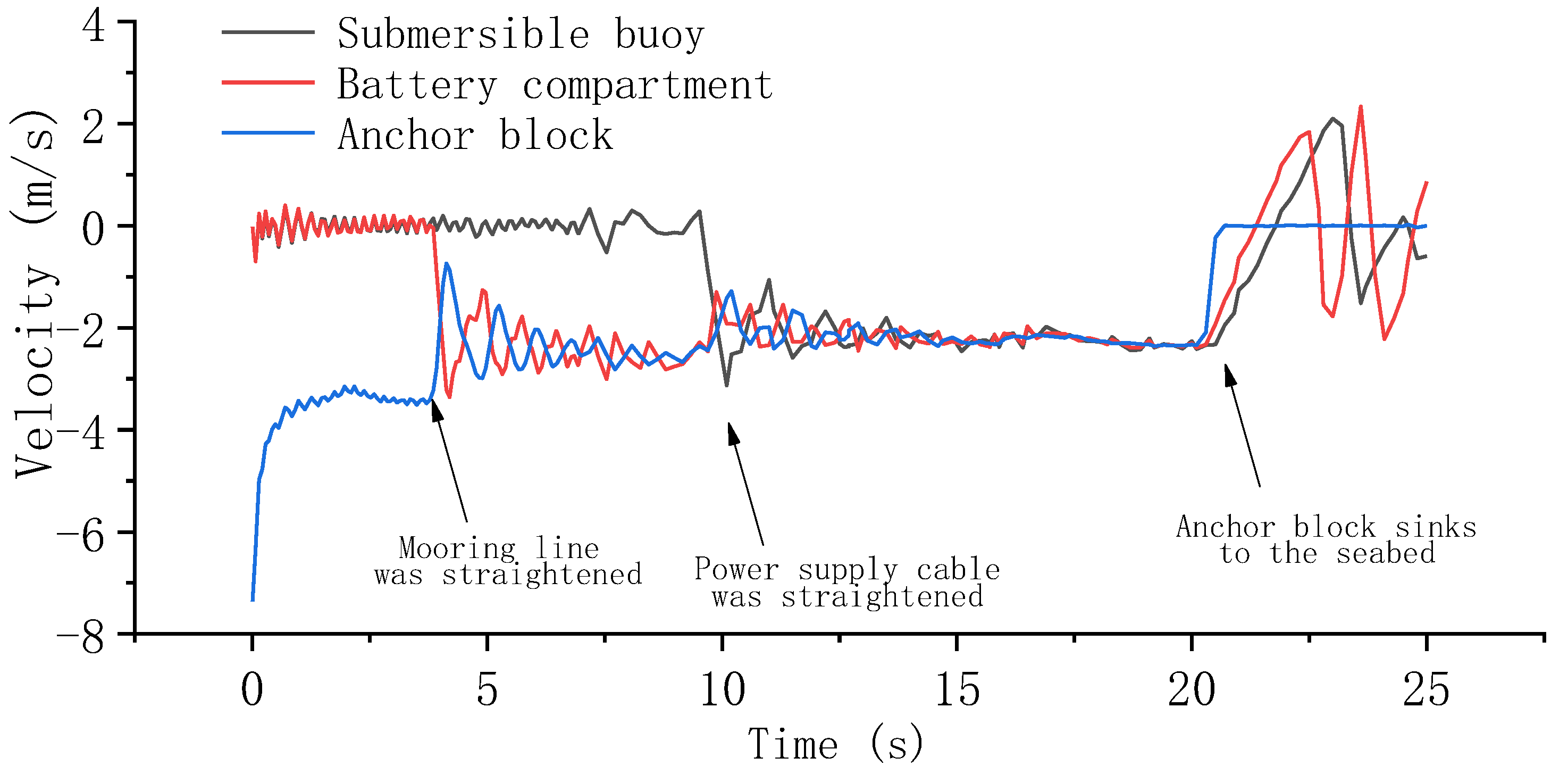
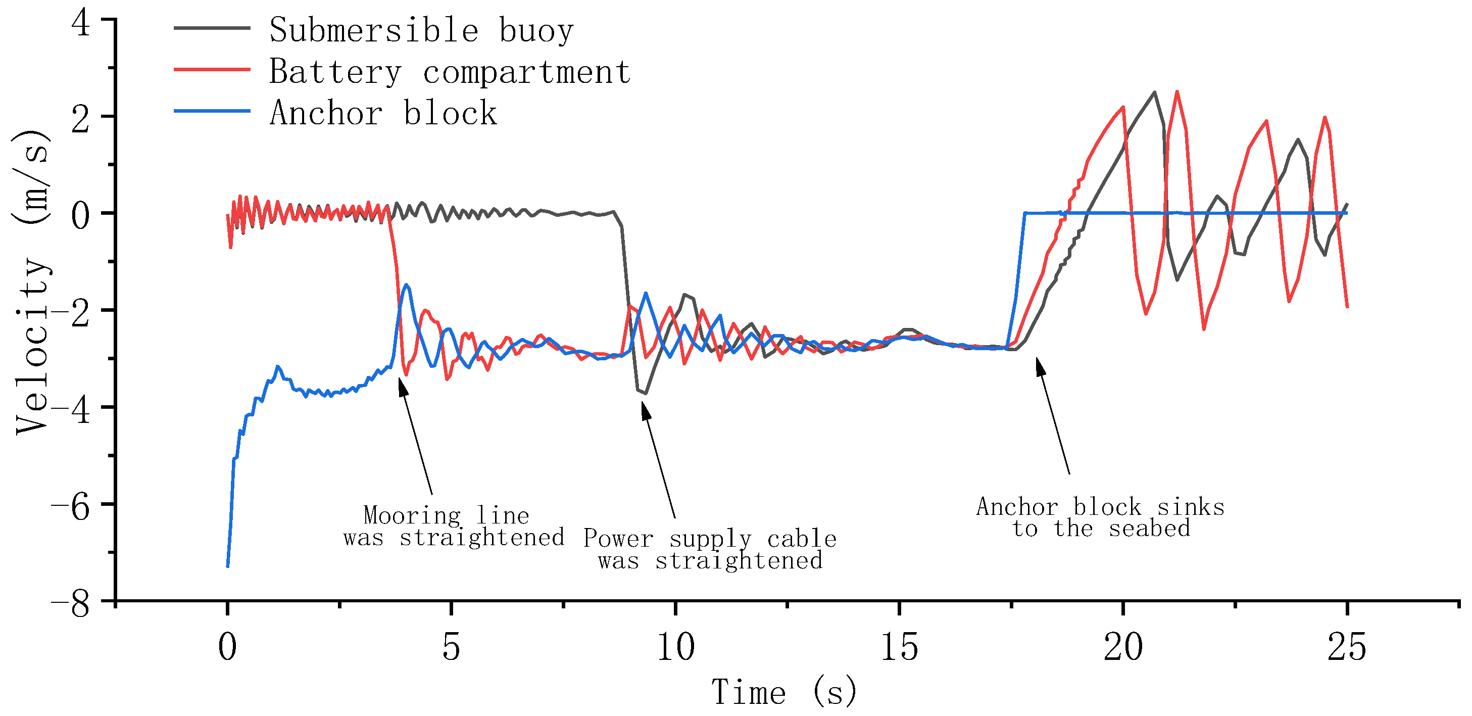
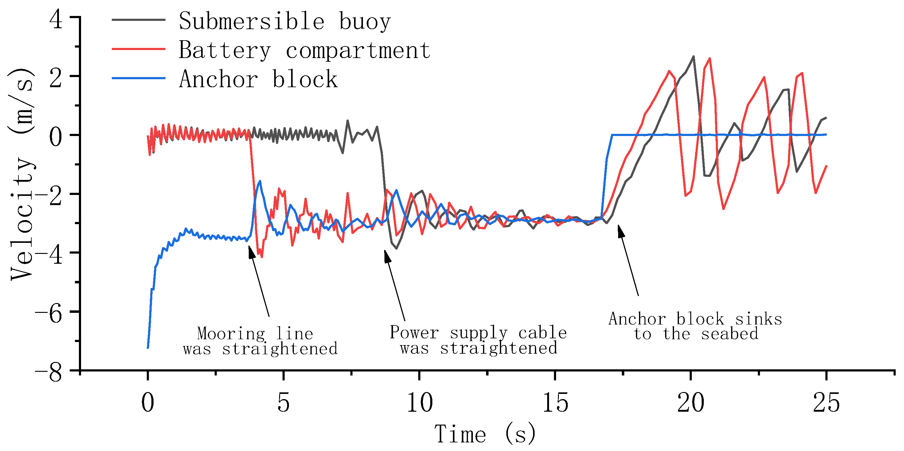
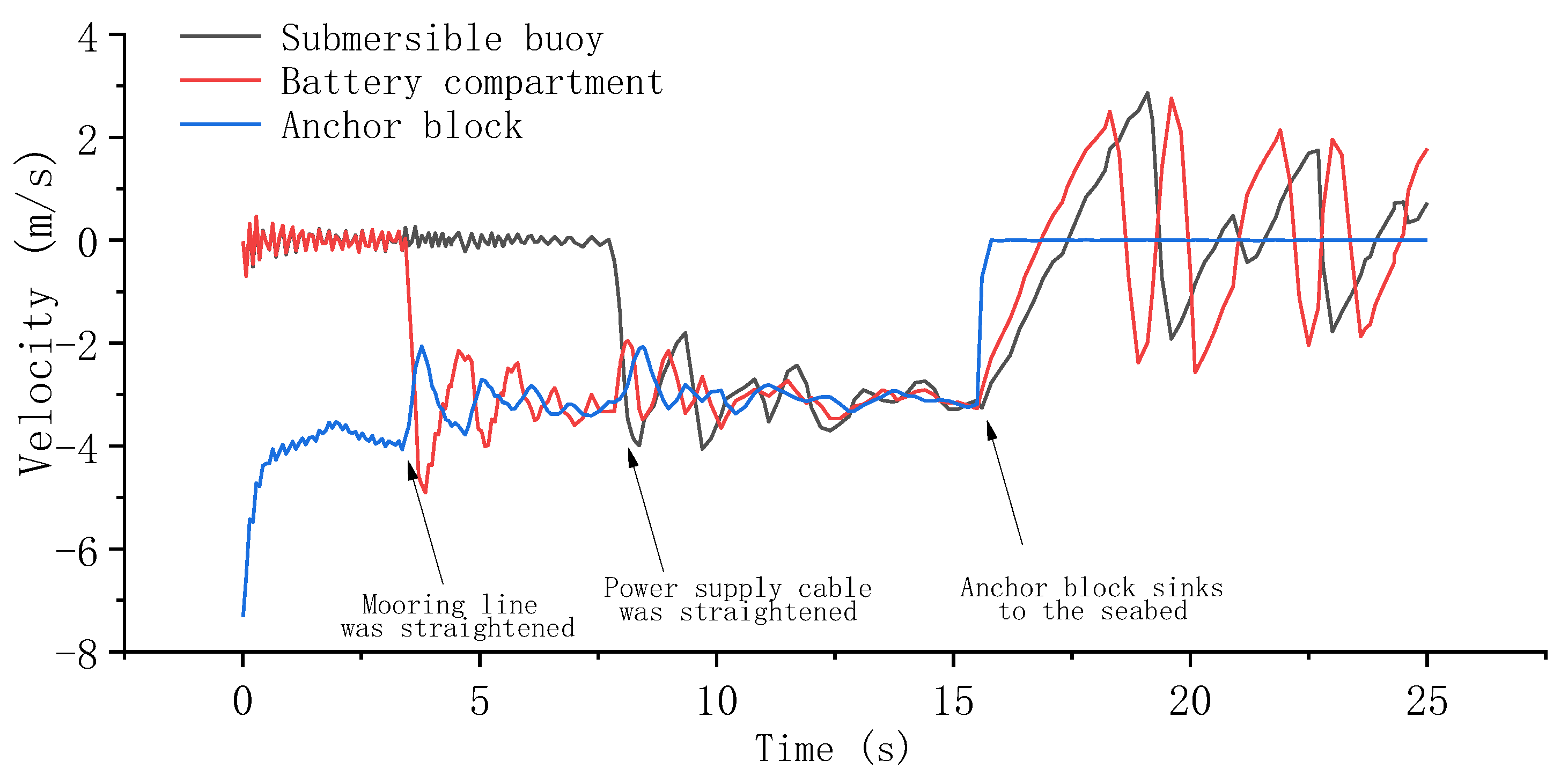
6.1. System Velocity Variation

Figure 10, Figure 11, Figure 12 and Figure 13 illustrate the velocity variation of the submersible buoy, battery compartment, and anchor block. After the anchor block enters the water, its velocity decreases rapidly to a stable value and then pulls the battery compartment and the submersible buoy into the water. The velocity of the battery compartment and the submersible buoy grow rapidly as they are pulled into the water, then exhibit a tendency of oscillation after entering the water. The amplitude of vibration changes gradually to a steady state. After the anchor block falls to the sea bed, the velocity of the anchor block rapidly decreases to zero, followed by a slight variation around zero because of the positive buoyancy of the submersible buoy and the battery compartment. The velocity of the submersible buoy and the battery compartment shows a trend of oscillation decreasing. The deployment under the different weights of the anchor block presents similar velocity change patterns.

After the power supply cable is straightened, the average velocity of the system after reaching the steady state is, respectively, 2.26 m/s, 2.69 m/s, 2.91 m/s, and 3.01 m/s. The steady velocity increases with the weight of the anchor block.

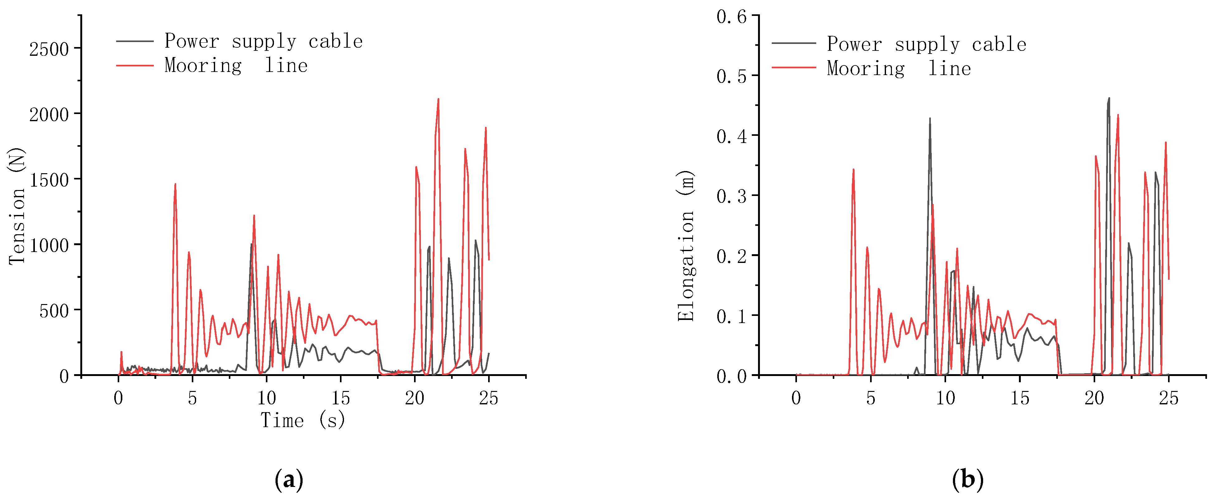
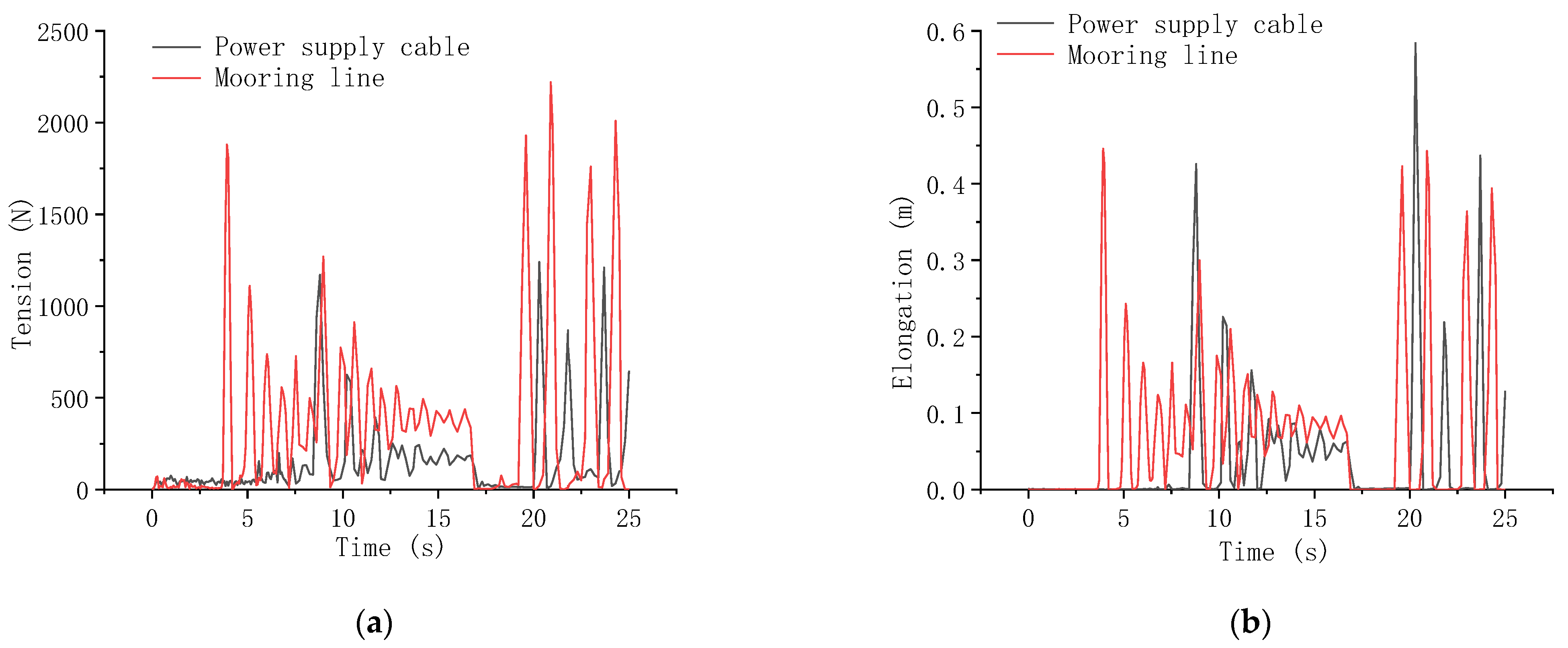
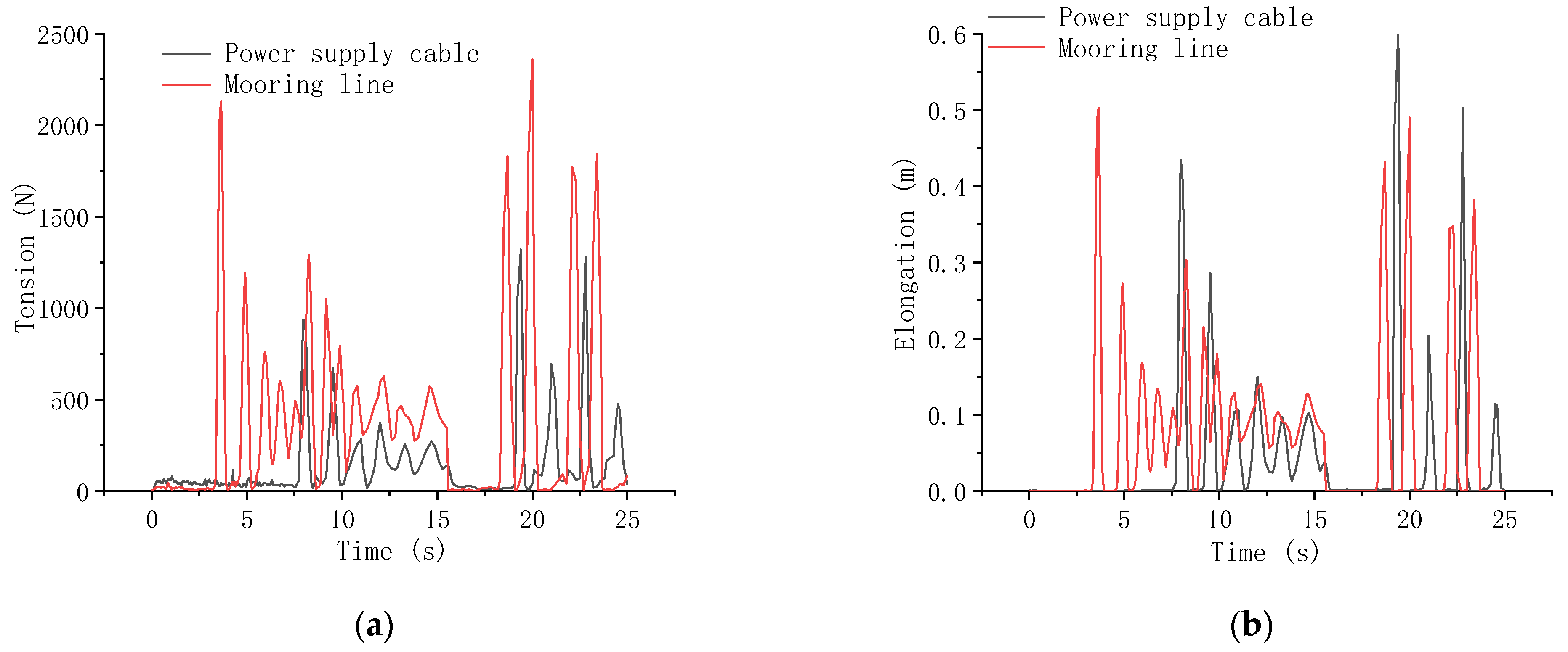
6.2. Cables Tension Variation

Figure 14, Figure 15, Figure 16 and Figure 17 illustrate the tension variation of the cables. Just as expected, a large tension occurs when the mooring line and power supply cable straighten. Then the tension and elongation oscillate to a stable value. The tension on the cables is relevant to the weight of the anchor block. In general, the greater the weight of the anchor block, the greater the tension and elongation.

After the anchor block sinks to the seabed, the positive buoyancy of the battery compartment and the buoy will cause large tension on the mooring line and power supply cable. The pulling force is higher than when the cables are straightened by the anchor block, which should be noted in the design process of marine submersible buoy systems.

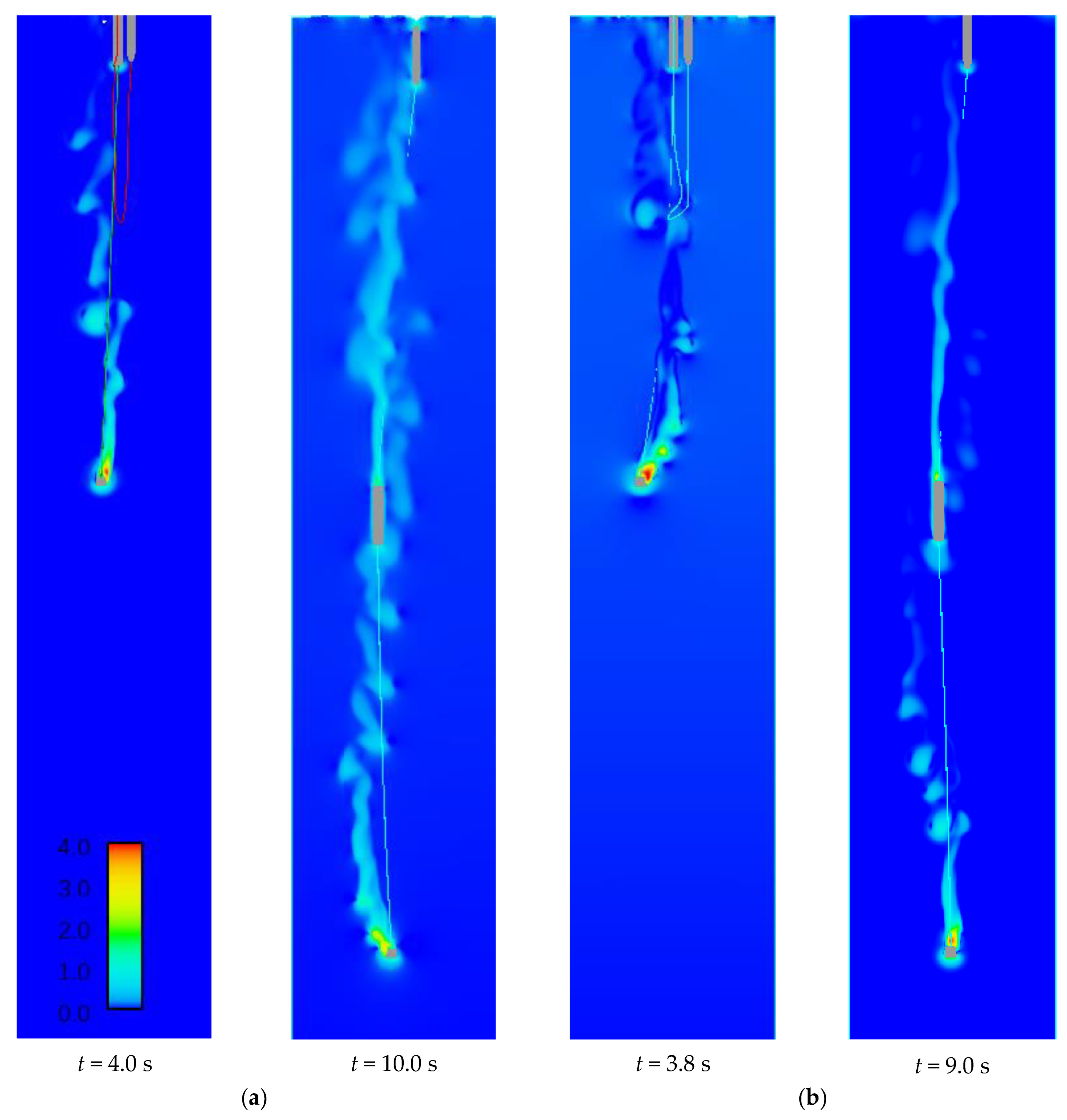
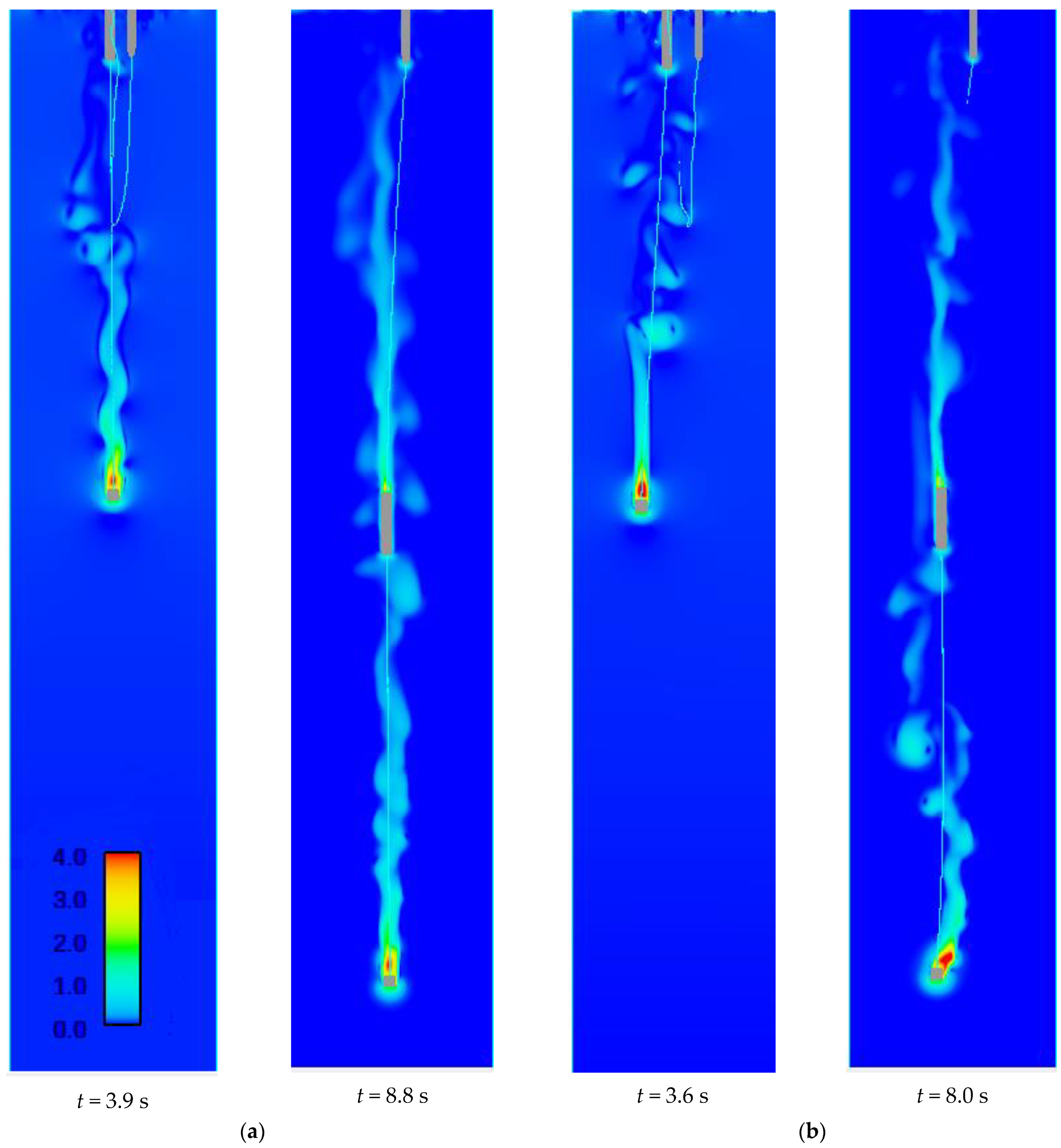
6.3. Fluid Velocity Variation during Deployment

The fluid velocity variation was shown in Figure 18 and Figure 19. The different colors in the figures means different velocity of fluid. The color chart show colors corresponding to different velocity. It can be seen from the results that boundary layer separation occurs in the anchor last deployment process. The tension of the mooring line and power supply cable change because of the boundary layer separation. The anchor block and the battery compartment change the fluid velocity in the tail trace. It is helpful to reduce the resistance of submersible buoys.

7. Conclusions

This paper established a computational fluid dynamic model of a marine submersible buoy system to study the anchor last deployment process. We used the VOF method to track the water entry process and used the lumped mass method to simulate the cables. The velocity variation of the three components, the mechanical behavior, and the fluid velocity variation were obtained by numerical simulation.

After the anchor block enters the water, the velocity decreases rapidly, then pulls the battery compartment and the submersible buoy into the water. The velocity of the battery compartment and the submersible buoy grows rapidly as they are pulled into the water, then exhibit a tendency of oscillation. After the anchor block falls to the seabed, the velocity of the submersible buoy and the battery compartment shows a trend of oscillation decreasing. The steady velocity increases with the weight of the anchor block.

When the mooring line and power supply cable are straight, there is large tension. Then the tension and elongation oscillate to a stable value. Tension on the mooring line and the power supply cable is relevant to the weight of the anchor block. In general, the greater the weight of the anchor block, the greater the tension and elongation on the mooring line and the power supply cable when straight.

Boundary layer separation occurs in the deployment process, which causes a variation in the tension on the cables. The tail trace is helpful to reduce the resistance of submersible buoys.

Using computational fluid dynamics to study the anchor last deployment process has some advantages. It can simulate the free fluid surface and the tail trace. However, the calculation is time-consuming. Some simplified methods in future research are proposed.

References

1. Li, F.Q.; Zhang, X.M.; Zhang, P.; Shen, G. The Design and Application of Marine Submersible Buoy System. Ocean Technol. 2004, 23, 17–21. [Google Scholar]
2. Hamilton, A.; Chaffey, M.; Mellinger, E.; Erickson, J.; Mcbride, L. Dynamic Modeling and Actual Performance of the MOOS Test Mooring. In Proceedings of the Oceans 2003, Celebrating the Past… Teaming toward the Future, San Diego, CA, USA, 22–26 September 2003; Volume 5, pp. 2574–2581. [Google Scholar] [CrossRef]
3. Augusto, O.B.; Andrade, B.L. Anchor Deployment for Deep Water Floating Offshore Equipments. Ocean Eng. 2003, 30, 611–624. [Google Scholar] [CrossRef]
4. Gobat, J.I.; Grosenbaugh, M.A. Time-Domain Numerical Simulation of Ocean Cable Structures. Ocean Eng. 2006, 33, 1373–1400. [Google Scholar] [CrossRef]
5. Chang, Z.; Tang, Y.; Li, H.; Yang, J.; Wang, L. Analysis for the Deployment of Single-Point Mooring Buoy System Based on Multi-Body Dynamics Method. China Ocean Eng. 2012, 26, 495–506. [Google Scholar] [CrossRef]
6. Zheng, Z.Q.; Dai, Y.; Gao, D.X.; Zhao, X.L.; Chang, Z.Y. Dynamics of Deployment for Mooring Buoy System Based on ADAMS Environment. Adv. Mater. Res. 2013, 819, 328–333. [Google Scholar] [CrossRef]
7. Zheng, Z.; Xu, J.; Huang, P.; Wang, L.; Yang, X.; Chang, Z. Dynamics of Anchor Last Deployment of Submersible Buoy System. J. Ocean Univ. China 2016, 15, 69–77. [Google Scholar] [CrossRef]
8. Yu, Y.; Zhao, T.; Duan, M.; Zhou, T.; Xu, J.; Su, Y.; Zhong, Z.; Liu, H. Experimental Investigation on the Underwater Soft Yoke Mooring System Considering Sloshing. Ships Offshore Struct. 2019, 14, 309–319. [Google Scholar] [CrossRef]
9. Yang, Q.; Zheng, Y.; Wang, Z.; Zhang, Y.; Hao, Z. The Influence of Vertical Cable on Flow Field and Acoustic Analysis of A Submersible Buoy System Based on CFD. In Proceedings of the 2019 14th IEEE Conference on Industrial Electronics and Applications (ICIEA), Xi’an, China, 19–21 June 2019; pp. 53–57. [Google Scholar] [CrossRef]
10. Tang, W.; Zhuang, H.; Tang, Z.; Guo, S.; Yan, F. Mooring Positioning Performance of Jack-up Platform. Ships Offshore Struct. 2020, 15, 633–644. [Google Scholar] [CrossRef]
11. Touzon, I.; Nava, V.; Gao, Z.; Mendikoa, I.; Petuya, V. Small Scale Experimental Validation of a Numerical Model of the HarshLab2.0 Floating Platform Coupled with a Non-Linear Lumped Mass Catenary Mooring System. Ocean Eng. 2020, 200, 107036. [Google Scholar] [CrossRef]
12. Chandrasekaran, S.; Uddin, S.A.; Wahab, M. Dynamic Analysis of Semi-Submersible Under the Postulated Failure of Restraining System with Buoy. Int. J. Steel Struct. 2021, 21, 118–131. [Google Scholar] [CrossRef]
13. Jiang, C.; el Moctar, O.; Schellin, T.E.; Paredes, G.M. Comparative Study of Mathematical Models for Mooring Systems Coupled with CFD. Ships Offshore Struct. 2021, 16, 942–954. [Google Scholar] [CrossRef]
14. Yang, R.-Y.; Chiang, W.-C. Dynamic Motion Response of an Oil Tanker Moored with a Single Buoy under Different Mooring System Failure Scenarios. Ships Offshore Struct. 2022, 1–14. [Google Scholar] [CrossRef]
15. Amaechi, C.V.; Wang, F.; Ye, J. Numerical Studies on CALM Buoy Motion Responses and the Effect of Buoy Geometry Cum Skirt Dimensions with Its Hydrodynamic Waves-Current Interactions. Ocean Eng. 2022, 244, 110378. [Google Scholar] [CrossRef]
16. Amaechi, C.V.; Wang, F.; Ye, J. Experimental Study on Motion Characterisation of CALM Buoy Hose System under Water Waves. J. Mar. Sci. Eng. 2022, 10, 204. [Google Scholar] [CrossRef]
17. Neisi, A.; Ghassemi, H.; Iranmanesh, M.; He, G. Effect of the Multi-Segment Mooring System by Buoy and Clump Weights on the Dynamic Motions of the Floating Platform. Ocean Eng. 2022, 260, 111990. [Google Scholar] [CrossRef]
18. Hirt, C.W.; Sicilian, J.M. Porosity Technique for the Definition of Obstacles in Rectangular Cell Meshes. In Proceedings of the 4th International Conference on Numerical Ship Hydrodynamics, Washington, DC, USA, 24–27 September 1985; pp. 450–468. [Google Scholar]
19. Yakhot, V.; Orszag, S.A. Renormalization Group Analysis of Turbulence. I. Basic Theory. J. Sci. Comput. 1986, 1, 3–51. [Google Scholar] [CrossRef]
20. Yakhot, A.; Orszag, S.A.; Yakhot, V.; Israeli, M. Renormalization Group Formulation of Large-Eddy Simulations. J. Sci. Comput. 1989, 4, 139–158. [Google Scholar] [CrossRef]
21. Hirt, C.W.; Nichols, B.D. Volume of Fluid (VOF) Method for the Dynamics of Free Boundaries. J. Comput. Phys. 1981, 39, 201–225. [Google Scholar] [CrossRef]
22. Huang, S. Dynamic Analysis of Three-Dimensional Marine Cables. Ocean. Eng. 1994, 21, 587–605. [Google Scholar] [CrossRef]
23. He, C. Study on Multiphase Flow of Typical Body during Water Entry. Ph.D. Thesis, Harbin Institute of Technology, Harbin, China, June 2022. [Google Scholar]
Figure 1. Schematic diagram of the marine submersible buoy system.
Jmse 10 01681 g001
Figure 2. Schematic diagram of the anchor last deployment.
Jmse 10 01681 g002
Figure 3. Schematic diagram of lumped mass method.
Jmse 10 01681 g003
Figure 4. Comparison between experiment and simulation of water entry process.
Jmse 10 01681 g004
Figure 5. Ratio of displacement to diameter as a function of time.
Jmse 10 01681 g005
Figure 6. Initial state of anchor last deployment.
Jmse 10 01681 g006
Figure 7. Boundary condition of computational fluid dynamic model.
Jmse 10 01681 g007
Figure 8. Anchor block position changes comparison between different grid sizes.
Jmse 10 01681 g008
Figure 9. Battery compartment position changes comparison between different grid sizes.
Jmse 10 01681 g009
Figure 10. Velocity variation with 60 kg underwater net weight of anchor block.
Jmse 10 01681 g010
Figure 11. Velocity variation with 80 kg underwater net weight of anchor block.
Jmse 10 01681 g011
Figure 12. Velocity variation with 100 kg underwater net weight of anchor block.
Jmse 10 01681 g012
Figure 13. Velocity variation with 120 kg underwater net weight of anchor block.
Jmse 10 01681 g013
Figure 14. Maximum tension of mooring line and power supply cable with 60 kg underwater net weight of anchor block: (a) Tension; (b) Elongation.
Jmse 10 01681 g014
Figure 15. Maximum tension of mooring line and power supply cable with 80 kg underwater net weight of anchor block: (a) Tension; (b) Elongation.
Jmse 10 01681 g015
Figure 16. Maximum tension of mooring line and power supply cable with 100 kg underwater net weight of anchor block: (a) Tension; (b) Elongation.
Jmse 10 01681 g016
Figure 17. Maximum tension of mooring line and power supply cable with 120 kg underwater net weight of anchor block: (a) Tension; (b) Elongation.
Jmse 10 01681 g017
Figure 18. The velocity of fluid when the mooring line and power supply cable were straight: (a) 60 kg underwater net weight of anchor block; (b) 80 kg underwater net weight of anchor block.
Jmse 10 01681 g018
Figure 19. The velocity of fluid when the mooring line and power supply cable were straight: (a) 100 kg underwater net weight of anchor block; (b) 120 kg underwater net weight of anchor block.
Jmse 10 01681 g019