
Numerical Investigation of Vortex-Induced Vibration of a Circular Cylinder with Control Rods and Its Multi-Objective Optimization


Abstract
1. Introduction
1.1. Vortex-Induced Vibration Suppression
1.2. Purpose of This Paper
2. Methodology
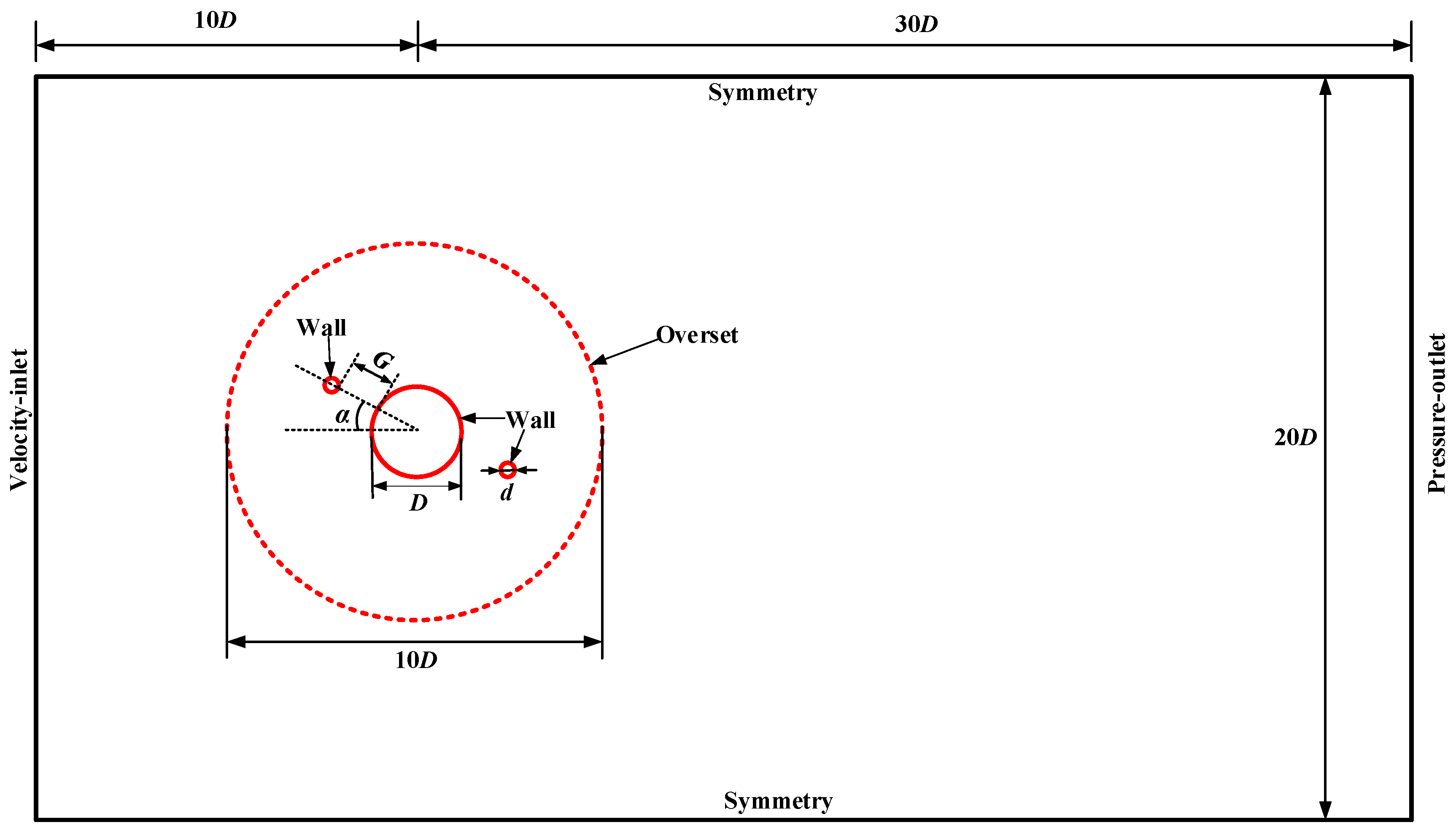
2.1. Physical Model
2.2. Governing Equations
- (1)
- Mass and momentum conservation equation
- (2)
- Turbulence model
- (3)
- Motion equation
2.3. Simulation Method
2.4. Validity of Numerical Scheme
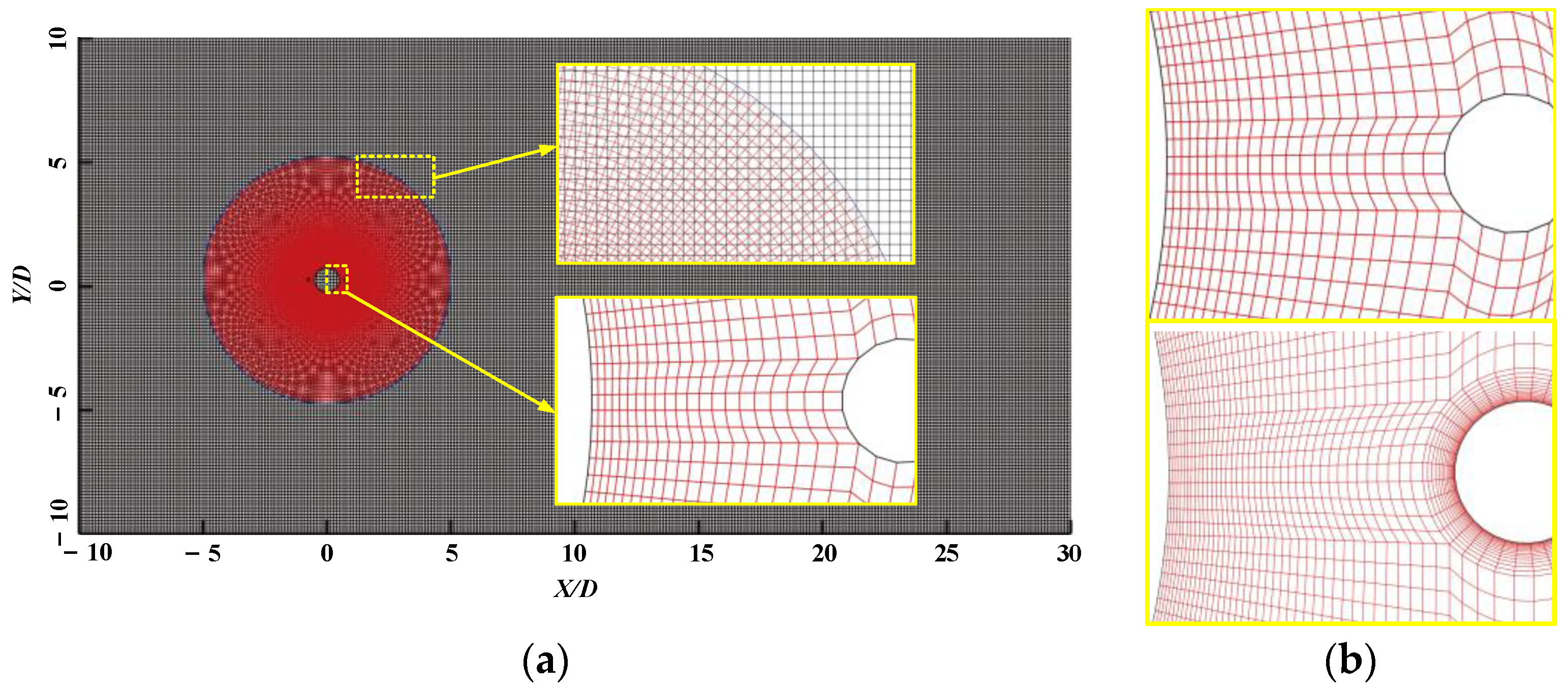
2.4.1. Meshing and Mesh Independence Check
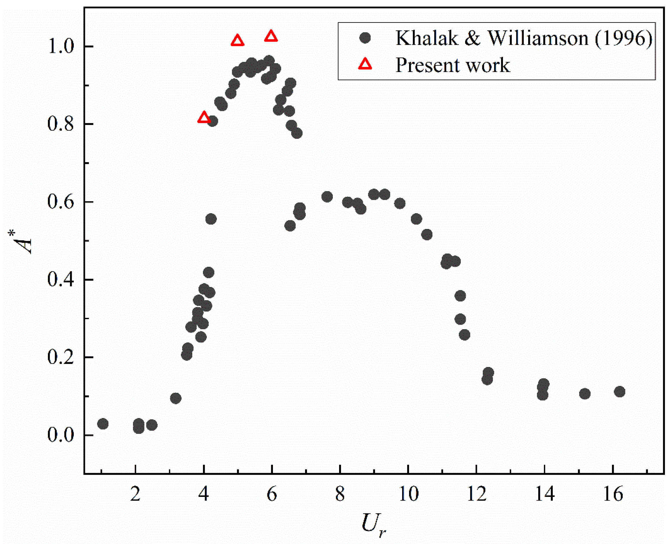
2.4.2. Numerical Validation
2.5. Response Surface Methodology
2.6. Genetic Algorithms
3. Results and Discussion
3.1. Multi-Objective Optimization
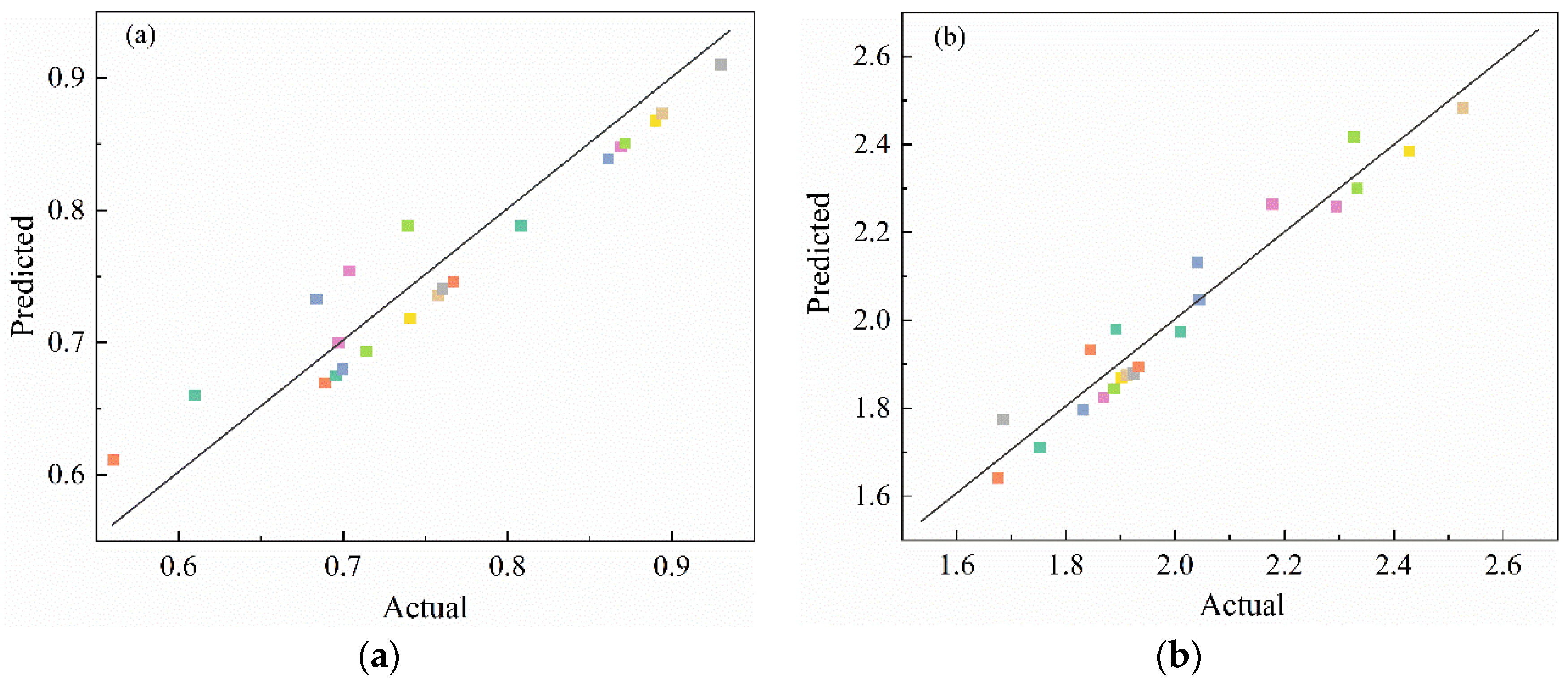
3.1.1. Response Surface Analysis
3.1.2. Optimization Using NSGA-II
3.2. Verification of Optimization Results and Comparison Flow Fields
3.2.1. Comparison and Verification
3.2.2. Flow Patterns before and after Optimization
4. Conclusions
- (1)
- The response surfaces show that there is an extreme value of A* under different combinations of variables. Among them, d/D shows a different synergistic effect from the other two variables. When d/D = 0.1, G/D achieves the minimum value of A* at the median value; when d/D = 0.3, G/D achieves the minimum value of A* at the upper limit and displays a monotonically decreasing trend. Unlike A*, the extreme point of CD occurs in the case of larger d/D and α, and small G/D.
- (2)
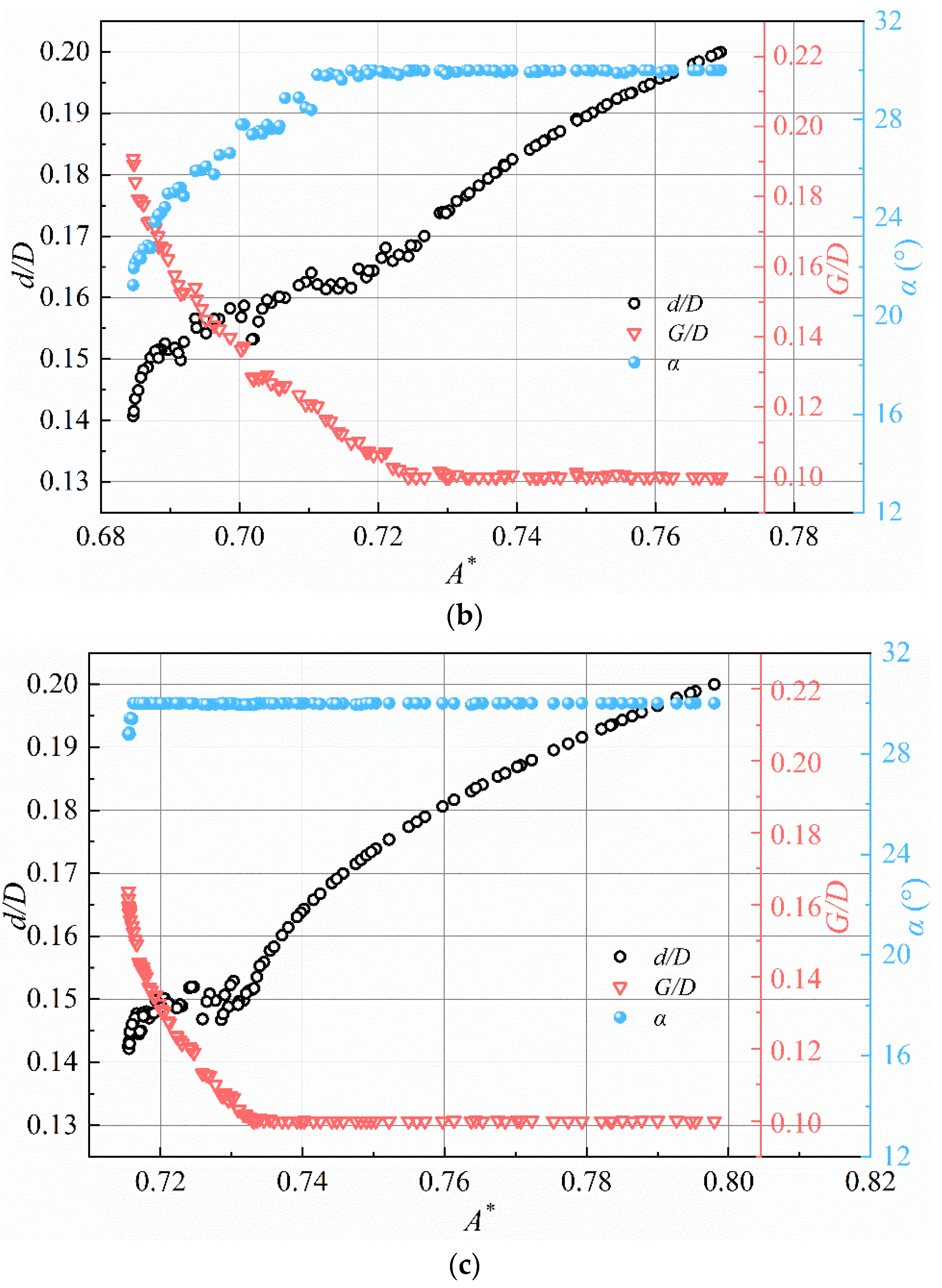
- The multi-objective optimization based on NSGA-II gives a series of Pareto optimal solutions for different reduced velocities (Ur = 4, 5, and 6). In general, the optimal design points of d/D all form a monotonically increasing relationship with A*, irrespective of reduced velocity. However, G/D and α will reach a stable design point with the increase in A*. Compared with the original cases, the values of A* after optimization are reduced by 15.1%, 24.8%, and 21.6% for Ur = 4, 5, and 6, respectively.
- (3)
- After the multi-objective optimization, the design variables d/D, G/D, and α reach the design points, and the objectives A* and CD also achieve the Pareto front at different Ur. These results can provide a useful reference for the optimal design of the cylinder rods body to suppress VIV.
Author Contributions
Funding
Institutional Review Board Statement
Informed Consent Statement
Data Availability Statement
Conflicts of Interest
References
- Yayli, M. Axial vibration analysis of a Rayleigh nanorod with deformable boundaries. Microsyst. Technol. 2020, 26, 2661–2671. [Google Scholar] [CrossRef]
- Yayli, M. Torsional vibration analysis of nanorods with elastic torsional restraints using non-local elasticity theory. Micro Nano Lett. 2018, 13, 595–599. [Google Scholar] [CrossRef]
- Yayli, M. Free vibration analysis of a rotationally restrained (FG) nanotube. Microsyst. Technol. 2019, 25, 3723–3734. [Google Scholar] [CrossRef]
- Wang, W.Q.; Yu, Z.F.; Gao, Y.; Luo, J.L.; Cao, W.Z. Study on the hydrodynamic characteristics of a marine riser under periodic pulsation disturbance. Ocean. Eng. 2021, 223, 108696. [Google Scholar] [CrossRef]
- Wang, D.; Hao, Z.F.; Pavloskaia, E.; Wiercigroch, M. Bifurcation analysis of vortex-induced vibration of low-dimensional models of marine risers. Nonlinear Dyn. 2021, 106, 147–167. [Google Scholar] [CrossRef]
- Yan, S.T.; Zhu, Y.F.; Jin, Z.J.; Ye, H. Buckle propagation analysis of deep-water petroleum transmission pipelines with axial tension. Adv. Mater. Res. 2014, 1008–1009, 1134–1143. [Google Scholar] [CrossRef]
- Faucher, V.; Ricciardi, G.; Boccaccio, R.; Cruz, K.; Lohez, T.; Clément, S.A. Numerical implementation and validation of a porous approach for fluid-structure interaction applied to pressurized water reactors fuel assemblies under axial water flow and dynamic excitation. Int. J. Numer. Methods Eng. 2021, 122, 2417–2445. [Google Scholar] [CrossRef]
- Mao, X.R.; Zhang, L.; Hu, D.J.; Ding, L. Flow induced motion of an elastically mounted trapezoid cylinder with different rear edges at high Reynolds numbers. Fluid Dyn. Res. 2019, 51, 025509. [Google Scholar] [CrossRef]
- Wang, X.K.; Wang, C.; Li, Y.L.; Tan, S.K. Flow patterns of a low mass-damping cylinder undergoing vortex-induced vibration: Transition from initial branch and upper branch. Appl. Ocean. Res. 2017, 62, 89–99. [Google Scholar] [CrossRef]
- Wang, X.K.; Hao, Z.; Tan, S.K. Vortex-induced vibrations of a neutrally buoyant circular cylinder near a plane wall. J. Fluids Struct. 2013, 39, 188–204. [Google Scholar] [CrossRef]
- Assi, G.R.S.; Bearman, P.W.; Kitney, N. Low drag solutions for suppressing vortex-induced vibration of circular cylinders. J. Fluids Struct. 2009, 25, 666–685. [Google Scholar] [CrossRef]
- Hwang, J.Y.; Yang, K.S.; Sun, S.H. Reduction of flow-induced forces on circular cylinder using a detached splitter plater. Phys. Fluids 2003, 15, 2433–2436. [Google Scholar] [CrossRef]
- Assi, G.R.S.; Bearman, P.W.; Kitney, N. Transverse galloping of circular cylinders fitted with solid and slotted splitter plates. J. Fluids Struct. 2015, 25, 666–675. [Google Scholar] [CrossRef]
- Wu, C.J.; Wang, L.; Wu, J.Z. Suppression of the von Karman vortex street behind a circular cylinder by travelling wave generated by a flexible surface. J. Fluid Mech. 2007, 574, 365–391. [Google Scholar] [CrossRef]
- Xu, F.; Chen, W.-L.; Xiao, Y.-Q.; Li, H.; Ou, J.-P. Numerical study on the suppression of the vortex-induce vibration of an elastically mounted cylinder by a traveling wave wall. J. Fluids Struct. 2014, 44, 389–447. [Google Scholar] [CrossRef]
- Lesage, F.; Gartshore, I.S. A method of reducing drag and fluctuating side force on bluff bodies. J. Wind. Eng. Ind. Aerodyn. 1987, 25, 229–245. [Google Scholar] [CrossRef]
- Igarashi, T.; Tsutsui, T. Flow control around a circular cylinder by a new method (2nd report, fluids forces acting on the cylinder). Trans. JSME 1989, 55, 708–714. [Google Scholar] [CrossRef]
- Dalton, C.; Xu, Y. The suppression of lift on a circular cylinder due to vortex shedding at moderate Reynolds numbers. J. Fluids Struct. 2001, 15, 617–628. [Google Scholar] [CrossRef]
- Wu, H.; Sun, D.; Lu, L.; Teng, B.; Tang, G.; Song, J. Experimental investigation on the suppression of vortex-induced vibration of long flexible riser by multiple control rods. J. Fluid Struct. 2012, 30, 115–132. [Google Scholar] [CrossRef]
- Zhu, H.J.; Yao, J. Numerical evaluation of passive control of VIV by small control rods. Appl. Ocean. Res. 2015, 51, 93–116. [Google Scholar] [CrossRef]
- Ong, M.C.; Utnes, T.; Holmedal, L.E.; Myrhaug, D.; Pettersen, B. Numerical simulation of flow around a smooth circular cylinder at very high Reynolds numbers. Mar. Struct. 2009, 22, 142–153. [Google Scholar] [CrossRef]
- Dey, P.; Das, A.K. Prediction and optimization of unsteady forced convection around a rounded cornered square cylinder in the range of Re. Neural Comput. Appl. 2017, 28, 1503–1513. [Google Scholar] [CrossRef]
- Pan, Z.Y.; Cui, W.C.; Miao, Q.M. Numerical simulation of vortex-induced vibration of a circular cylinder at low mass-damping using RANS code. J. Fluids Struct. 2007, 23, 23–37. [Google Scholar] [CrossRef]
- Khalak, A.; Williamson, C.H.K. Fluid forces and dynamics of hydroelastic structure with very low mass and damping. J. Fluids Struct. 1997, 11, 937–982. [Google Scholar] [CrossRef]
- Prasanth, T.K.; Mittal, S. Vortex-induced vibration of two circular cylinders at low Reynolds number. J. Fluids Struct. 2009, 25, 731–741. [Google Scholar] [CrossRef]
- Papaioannou, G.V.; Yue, D.K.P.; Triantafyllou, M.S.; Karniadakis, G.E. On the effect of spacing on the vortex induced vibrations of two tandem cylinders. J. Fluids Struct. 2008, 24, 833–854. [Google Scholar] [CrossRef]
- Khalak, A.; Williamson, C.H.K. Dynamics of a hydroelastic cylinder with very low and damping. J. Fluids Struct. 1996, 10, 455–472. [Google Scholar] [CrossRef]
- Sankar, P.S.; Prasad, R.K. Process modeling and particle flow simulation of sand separation in cyclone separator. J. Part. Sci. Technol. 2015, 33, 385–392. [Google Scholar] [CrossRef]
- Sun, X.; Kim, S.; Yang, S.D.; Kim, H.S.; Yoon, J.Y. Multi-objective optimization of a Stairmand cyclone separator using Response Surface Methodology and computational fluid dynamics. J. Powder Technol. 2017, 320, 51–65. [Google Scholar] [CrossRef]
- Rahmani, S.; Mousavi, S.M.; Kamali, M.J. Modeling of road-traffic noise with the use of genetic algorithm. J. Appl. Soft Comput. 2011, 11, 1008–1013. [Google Scholar] [CrossRef]
- Deb, K.; Pratap, A.; Agarwal, S.; Meyarivan, T. A fast and elitist multi-objective genetic algorithm: NSGA-II. J. IEEE Trans. Evol. Comput. 2002, 6, 182–197. [Google Scholar] [CrossRef]
- Wang, B.; Xu, D.L.; Chu, K.W.; Yu, A.B. Numerical study of gas-solid flow in a cyclone separator. J. Appl. Math. Model. 2006, 30, 1326–1342. [Google Scholar] [CrossRef]
- Sakamoto, H.; Haniu, H. Optimum suppression of fluid forces acting on a circular cylinder. J. Fluids Eng. 1994, 116, 221–227. [Google Scholar] [CrossRef]
- Zhao, M.; Cheng, L.; Teng, B.; Liang, D.F. Numerical simulation of viscous flow past two circular cylinders of different diameters. Appl. Ocean. Res. 2005, 27, 39–55. [Google Scholar] [CrossRef]
- Morse, T.L.; Williamson, C.H.K. Fluid forcing, wake modes, and transitions for a cylinder undergoing controlled oscillations. J Fluid Struct. 2009, 25, 617–712. [Google Scholar] [CrossRef]


| Mesh | Number of Elements | A* | CD |
|---|---|---|---|
| M1 | 24132 | 0.724 | 2.443 |
| M2 | 36706 | 0.815 | 2.612 |
| M3 | 49380 | 0.981 | 2.946 |
| M4 | 70236 | 1.013 | 3.041 |
| M5 | 107112 | 1.017 | 3.062 |
| Design Parameters | Level | ||
|---|---|---|---|
| −1 | 0 | 1 | |
| Diameter ratio (d/D) | 0.1 | 0.15 | 0.2 |
| Gap ratio (G/D) | 0.1 | 0.2 | 0.3 |
| Incidence angle (α, °) | 0 | 15 | 30 |
| Reduced velocity (Ur) | 4 | 5 | 6 |
| Run No. | Cylinder Rods Body Parameters | CFD Results | ||||
|---|---|---|---|---|---|---|
| d/D | G/D | α (°) | Ur | A* | CD | |
| 1 | 0.15 | 0.1 | 15 | 6 | 0.751 | 1.687 |
| 2 | 0.15 | 0.3 | 30 | 5 | 0.809 | 2.429 |
| 3 | 0.2 | 0.3 | 15 | 5 | 0.758 | 1.934 |
| 4 | 0.1 | 0.2 | 0 | 5 | 0.705 | 2.178 |
| 5 | 0.1 | 0.3 | 15 | 5 | 0.761 | 2.296 |
| 6 | 0.15 | 0.2 | 30 | 6 | 0.759 | 1.833 |
| 7 | 0.15 | 0.3 | 15 | 6 | 0.831 | 2.043 |
| 8 | 0.1 | 0.2 | 15 | 4 | 0.701 | 2.527 |
| 9 | 0.1 | 0.2 | 30 | 5 | 0.684 | 2.326 |
| 10 | 0.15 | 0.2 | 15 | 5 | 0.698 | 2.045 |
| 11 | 0.2 | 0.1 | 15 | 5 | 0.872 | 1.678 |
| 12 | 0.15 | 0.1 | 0 | 5 | 0.895 | 1.892 |
| 13 | 0.2 | 0.2 | 15 | 4 | 0.767 | 1.754 |
| 14 | 0.15 | 0.3 | 15 | 4 | 0.651 | 1.845 |
| 15 | 0.15 | 0.1 | 15 | 4 | 0.692 | 1.401 |
| 16 | 0.15 | 0.2 | 15 | 5 | 0.698 | 2.045 |
| 17 | 0.15 | 0.2 | 15 | 5 | 0.698 | 2.045 |
| 18 | 0.2 | 0.2 | 30 | 5 | 0.739 | 1.54 |
| 19 | 0.15 | 0.2 | 15 | 5 | 0.698 | 2.045 |
| 20 | 0.2 | 0.2 | 0 | 5 | 0.908 | 1.892 |
| 21 | 0.15 | 0.2 | 15 | 5 | 0.698 | 2.045 |
| 22 | 0.1 | 0.1 | 15 | 5 | 0.89 | 2.008 |
| 23 | 0.2 | 0.2 | 15 | 6 | 0.87 | 1.871 |
| 24 | 0.15 | 0.2 | 0 | 6 | 0.93 | 1.904 |
| 25 | 0.15 | 0.2 | 30 | 4 | 0.697 | 1.914 |
| 26 | 0.15 | 0.2 | 0 | 4 | 0.691 | 2.335 |
| 27 | 0.15 | 0.3 | 0 | 5 | 0.861 | 1.927 |
| 28 | 0.15 | 0.1 | 30 | 5 | 0.715 | 1.64 |
| 29 | 0.1 | 0.2 | 15 | 6 | 0.741 | 1.931 |
| Source | Vibration Amplitude | Drag Force Coefficient | ||||
|---|---|---|---|---|---|---|
| Sum of Squares | F-Value | p-Value | Sum of Squares | F-Value | p-Value | |
| d/D | 9.506 × 10⁻³ | 2.13 | 0.1952 | 0.17 | 11.86 | 0.0137 |
| G/D | 4.16 × 10⁻³ | 0.93 | 0.3721 | 0.16 | 10.94 | 0.0163 |
| α | 6.806 × 10⁻³ | 1.52 | 0.2635 | 0.061 | 4.14 | 0.0882 |
| Ur | 0.023 | 5.06 | 0.0654 | 0.066 | 4.48 | 0.0768 |
| Run. | Ur | d/D | G/D | α (°) | NSGA-II | CFD Results | Deviation (%) | ||||
|---|---|---|---|---|---|---|---|---|---|---|---|
| A* | CD | A* | CD | A* | CD | ||||||
| 1 | Before | 4 | 0.2 | 0.2 | 15 | / | / | 0.767 | 1.754 | / | / |
| 2 | After | 4 | 0.18 | 0.13 | 27.2 | 0.674 | 1.317 | 0.651 (↓ 15.1%) | 1.248 | 3.4% | 5.2% |
| 3 | Before | 5 | 0.1 | 0.1 | 15 | / | / | 0.89 | 2.008 | / | / |
| 4 | After | 5 | 0.15 | 0.17 | 24.1 | 0.688 | 1.907 | 0.669 (↓ 24.8%) | 1.846 | 2.7% | 3.2% |
| 5 | Before | 6 | 0.15 | 0.2 | 0 | / | / | 0.93 | 1.904 | / | / |
| 6 | After | 6 | 0.17 | 0.1 | 30 | 0.742 | 1.448 | 0.729 (↓ 21.6%) | 1.426 | 1.8% | 3% |
Publisher’s Note: MDPI stays neutral with regard to jurisdictional claims in published maps and institutional affiliations. |
© 2022 by the authors. Licensee MDPI, Basel, Switzerland. This article is an open access article distributed under the terms and conditions of the Creative Commons Attribution (CC BY) license (https://creativecommons.org/licenses/by/4.0/).
Share and Cite
Hu, Z.; Chen, J.; Qu, S.; Wang, X. Numerical Investigation of Vortex-Induced Vibration of a Circular Cylinder with Control Rods and Its Multi-Objective Optimization. J. Mar. Sci. Eng. 2022, 10, 1659. https://doi.org/10.3390/jmse10111659
Hu Z, Chen J, Qu S, Wang X. Numerical Investigation of Vortex-Induced Vibration of a Circular Cylinder with Control Rods and Its Multi-Objective Optimization. Journal of Marine Science and Engineering. 2022; 10(11):1659. https://doi.org/10.3390/jmse10111659
Chicago/Turabian StyleHu, Zhiyang, Jiaqi Chen, Sen Qu, and Xikun Wang. 2022. "Numerical Investigation of Vortex-Induced Vibration of a Circular Cylinder with Control Rods and Its Multi-Objective Optimization" Journal of Marine Science and Engineering 10, no. 11: 1659. https://doi.org/10.3390/jmse10111659
APA StyleHu, Z., Chen, J., Qu, S., & Wang, X. (2022). Numerical Investigation of Vortex-Induced Vibration of a Circular Cylinder with Control Rods and Its Multi-Objective Optimization. Journal of Marine Science and Engineering, 10(11), 1659. https://doi.org/10.3390/jmse10111659