Article

Numerical Simulation of Scalar Mixing and Transport through a Fishing Net Panel

1
State Key Laboratory of Water Environment Simulation & School of Environment, Beijing Normal University, Beijing 100875, China
2
Department of Civil, Architectural and Environmental Engineering, University of Naples Federico II, 80125 Napoli, Italy
3
School of Science and Engineering (Civil Engineering), University of Dundee, Dundee DD1 4HN, UK
4
Department of Civil and Environmental Engineering, Rutgers, The State University of New Jersey, Piscataway, NJ 08854, USA
*
Author to whom correspondence should be addressed.
Tang Scholar from the Tang Foundation.
J. Mar. Sci. Eng. 2022, 10(10), 1511; https://doi.org/10.3390/jmse10101511
Submission received: 31 August 2022 / Revised: 3 October 2022 / Accepted: 13 October 2022 / Published: 17 October 2022
(This article belongs to the Section Ocean Engineering)

Abstract

:
With the rapid development of commercial aquaculture in recent decades, large numbers of submerged cages or pens are clustered in fish farms that are commonly located within inland lakes, reservoirs, and coastal embayments around the world. The submerged structures have significant influence on both the flow fields and mass transport processes in surrounding water bodies. While existing studies have concentrated mainly on the flow blockage effects produced by fish cages, the associated effect on near-field mass transport processes, important for pollution transport and dispersal, remains largely unclear. To address this knowledge gap, a CFD (computational fluid dynamics) model was established using OpenFOAM to investigate the wake characteristics and scalar transport processes through a fishing net panel, as representative of a key component of the fish cage or pen. In this model, the net panel was represented as porous media, and the finite volume method was applied to solve the governing flow equations with the standard k-ε model used for turbulence closure. Experimental data from previous studies were used to calibrate and validate the numerical model, which was applied to different scenarios over a range of net solidities and incoming flow velocities. Overall, the numerical model results demonstrated that porous media schematization could adequately reproduce the blocking effect from the net panel on the mean flow field, as well as the induced changes to scalar transport, with satisfactory accuracy. The flow velocity reduction across the net panel was found to strengthen with increasing net solidity and decreasing incoming velocity, while the scalar concentration decay tended to become enhanced when the incoming velocity was decreased. The lateral profile of the scalar concentration exhibited a self-similar Gaussian distribution with the spreading width of the plume reduced by increasing the incoming velocity. This lateral concentration distribution was minimally affected by the upstream scalar source location relative to the net panel, when adopting the current RANS and porous media modelling approach. The model results provide useful references for the assessment of the environmental impacts and carrying capacity of cage-based fish farming.

1. Introduction

With the significant increase in global seafood demands in recent years, the aquaculture industry has expanded rapidly to contribute to more than half of the overall fish production worldwide [1]. As a result, a large number of cages or pens are often clustered within fish farms that are sited within inland lakes, reservoirs, and coastal embayments in many countries around the world. These submerged structures have a considerable impact on both the near-field hydrodynamics and mass transport processes within the surrounding waters in the vicinity of the cages/pens [2]. Specifically, both water exchange through the fish cage and the transport of oxygen, nutrients, wastes, pathogens, and medicinal treatments within the water column can be significantly impacted by the near-field flow characteristics [3]. This, in turn, can have significant impact on fish health and growth rate, as well as on the surrounding environmental water quality [4,5]. As a key component of the fish cage or pen, the fishing net panels have a highly porous structure that generate relatively complex wake flows, especially at scales close to the netting mesh sizes [6,7,8]. Understanding the near-field flow field and mass transport processes through an individual net panel is therefore a critical first step to the more complex study of larger-scale flows involving individual cage/pen structures or even groups of cages/pens.
Experimental studies on the flow field around a fish cage have been carried out extensively in the past several decades (see, for example, the review by [2]. The flow field around an individual fishing net panel has received less attention until relatively recently. Amongst the available studies, Lee et al. [9] measured the flow velocity before and after the net panel with three net solidities to investigate the shielding effect of the fish-cage system in currents. Cha et al. [10] used particle image velocimetry (PIV) to measure the flow through a copper alloy net, reporting that the hydrodynamic characteristics of the net were affected by its structural shape. Bi et al. [11] conducted a series of laboratory experiments to measure the flow velocity downstream of the fishing net panel in a constant flow using PIV and acoustic doppler velocimeter (ADV) measurement techniques. They found that the wake flow downstream of the net panel showed a marked reduction that increased with increasing net solidity and net inclination angle to the flow. More recently, Shao et al. [7] combined PIV and planar laser induced fluorescence (PLIF) flow imaging techniques to investigate experimentally the associated scalar transport process in the near-field wake of a steady current through a flexible net panel, observing that the presence of the net slightly enhanced the lateral spreading of the tracer plume. Zeng et al. [8] subsequently measured the corresponding flow field and associated scalar transport processes through a rigid planar metal net panel, finding that the rigid nets reduce flow blockage and increase the rate of concentration decay compared to flexible nets with a similar solidity. Notably, regarding the mass transport process through net structures, analogous studies on the scalar transport in grid-generated turbulence have been widely reported in the literature [12,13,14,15,16,17].
Significant progress has also been made on the numerical modelling of fishing nets associated with aquaculture. Among the relevant numerical studies, the net is typically schematized as a thin-volume porous medium with added resistance incorporated in the momentum equation to model flow through the fishing net [2,11,18,19,20,21,22]. Specifically, Patursson et al. [18] simulated the flow characteristics through and around a fishing net panel, and confirmed that the flow velocity reduced behind the net. Zhao et al. [19] developed a three-dimensional (3D) numerical model to simulate the flow field through and around the net with different net inclination angles, net heights, and spacing distances between two nets, also observing flow velocity reduction behind the net. In addition, other modelling approaches, such as analytical modelling [23] and a lattice Boltzmann model [24], have also been adopted successfully to simulate the flow field around fishing net panels.
The above studies have been focused mainly on numerical simulations of the flow field around the fishing net panel, while numerical studies on scalar transport through fishing net panels, complementary to recent experimental efforts, are still lacking. Following Batchelor [25], the downstream region in the immediate vicinity of the net (grids) (i.e., x/M ≤ 20, x being downstream distance and M being mesh size) was defined as the near-field, while the region further downstream (i.e., x/M > 20) was defined as the far-field. In the current study, numerical simulations were performed to explore the turbulent wake characteristics and scalar transport processes in both the near- and far-fields generated from flow through fishing net panels with different net solidities and incoming velocities. A three-dimensional numerical model was developed using OpenFOAM (File S1), an open-source computational fluid dynamics (CFD) toolbox that has gained increasing popularity within science and engineering communities in recent years for the study of environmental fluid mechanics problems. This modelling approach has also recently been applied successfully to investigate similar aquaculture-related hydrodynamics in culture tanks for Atlantic salmon [26]. Within the current numerical modelling study, we have used previous experimental data reported in Zeng et al. [8] to calibrate and validate the model, which was then applied to undertake extended scenario modelling. It is anticipated that the results from the study may provide new modelling perspectives on both the flow field and mass transport processes in the near-wake region of cage-based aquaculture.

2. Methodology

2.1. The Governing Equations

In the present study, the incompressible viscous flow field around the fishing net panel is described by the Reynolds-averaged Navier–Stokes (RANS) and advection–diffusion (ADE) equations. The governing equations, including the continuity (Equation (1)), momentum (Equation (2)), and the passive scalar transport (Equation (3)) equations are shown as follows [18,19,27]:
u i x i = 0
ρ u i t + ρ u i u j x j = P x i + x j μ + μ t u i x j + u j x i + S i
t + u j x j = x j Γ x j + S
where t is time; u i and u j are the time-averaged velocity components, respectively; i , j = x , y , z ; ρ is the density of the fluid; P = p + 2 / 3 ρ k , where P is the time-averaged pressure and k is the turbulent kinetic energy; μ is the dynamic viscosity of the fluid; μ t is the eddy viscosity of the fluid; S i is the source term for the momentum equation, which is used to account for the added fluid resistance force of the fishing net panel; is the concentration of the passive scalar; Γ is the turbulent or eddy diffusivity; and S is the source term for the scalar transport equation.
Patursson et al. [28] examined the dependence of using different k-ε turbulence models for 2D flow around net panels treated as porous media and found the difference to be small. Therefore, the standard k-ε model, a widely used RANS turbulence model [29], was adopted in the present study for turbulence closure. The equations describing turbulence kinetic energy k (Equation (4)) and its rate of dissipation ε (Equation (5)) are as follows [29]:
ρ k t + ρ k u i x i = x j μ + μ t σ k k x j + G k ρ ε
ρ ε t + ρ ε u i x i = x j μ + μ t σ ε k x j + C 1 ε G k ε k C 2 ε ρ ε 2 k
where G k = μ t u i x j + u j x i u i x j represents the generation of turbulence kinetic energy by the average velocity gradient; C 1 ε , C 2 ε are constants; and σ k and σ ε are the turbulent Prandtl numbers for k and ε, respectively. In the standard k-ε model, the turbulent viscosity μ t is a function of k and ε [29]:
μ t = ρ C μ k 2 ε
where C μ = 0.09 , σ k = 1.0 , σ ε = 1.3 , C 1 ε = 1.44 , C 2 ε = 1.92 are given by Launder and Spalding [29]. Turbulent diffusivity Γ is related to turbulent viscosity through their ratio, i.e., the turbulent Schmidt number S c t :
S c t = μ t ρ Γ
which was assumed to be constant throughout the domain. Hence, while eddy viscosity was calculated using Equation (6), the eddy diffusivity was estimated using Equation (7), where the value of S c t was calibrated against the near-field concentration measurements presented in Zeng et al. [8].

2.2. Porous Media Model

Following previous numerical studies [18,19], the fishing net panel was treated as porous media with a specified thickness and the same size and shape as the net panel. The source term that accounts for the added resistance of the net in the momentum equation can be expressed following the Darcy–Forchheimer Equation [18]:
S i = D i j μ u + C i j 1 2 ρ u u
where D i j and C i j are prescribed matrices consisting of the resistance coefficients in the principal axes of the porous media:
D i j = D n 0 0 0 D t 0 0 0 D t ; C i j = C n 0 0 0 C t 0 0 0 C t
where D n and D t are the normal and tangential viscous resistance coefficients, respectively; and C n and C t are the normal and tangential inertia resistance coefficients, respectively. D t and C t can be ignored when the net is oriented normal to the flow. Moreover, for fully turbulent flow through the net, the linear viscous term is dominated by the quadratic inertia term and thus can be neglected [30,31]. Thus,
S i = 1 2 C n ρ u u
For flow through the porous media, the resistance force F acting on the fluid from the porous media in the i direction can be written as follows [19,20]:
F = S i λ A
where λ is the thickness of the fishing net panel, and A is the area of the fishing net panel. Here, the magnitude of resistance force F equals to the drag force on the fishing net panel in the streamwise direction. Thus, substituting Equation (10) into Equation (11) leads to:
F d = 1 2 C n ρ u u λ A
In addition, the drag force on the fishing net panel can also be expressed from the Morison equation [32]:
F d = 1 2 C d ρ u 2 A
where C d is the drag coefficient. According to Equations (12) and (13), the porous media coefficient C n is related to C d as follows:
C n = C d λ
Notably, a number of previous studies have developed empirical formulas for C d as a function of both net properties and flow characteristics and summarized by Klebert et al. [2]. In this study, the values of C n for calibration cases were determined against corresponding experimental data in Zeng et al. [8], and further compared with the empirical formula from Klebert et al. [2].

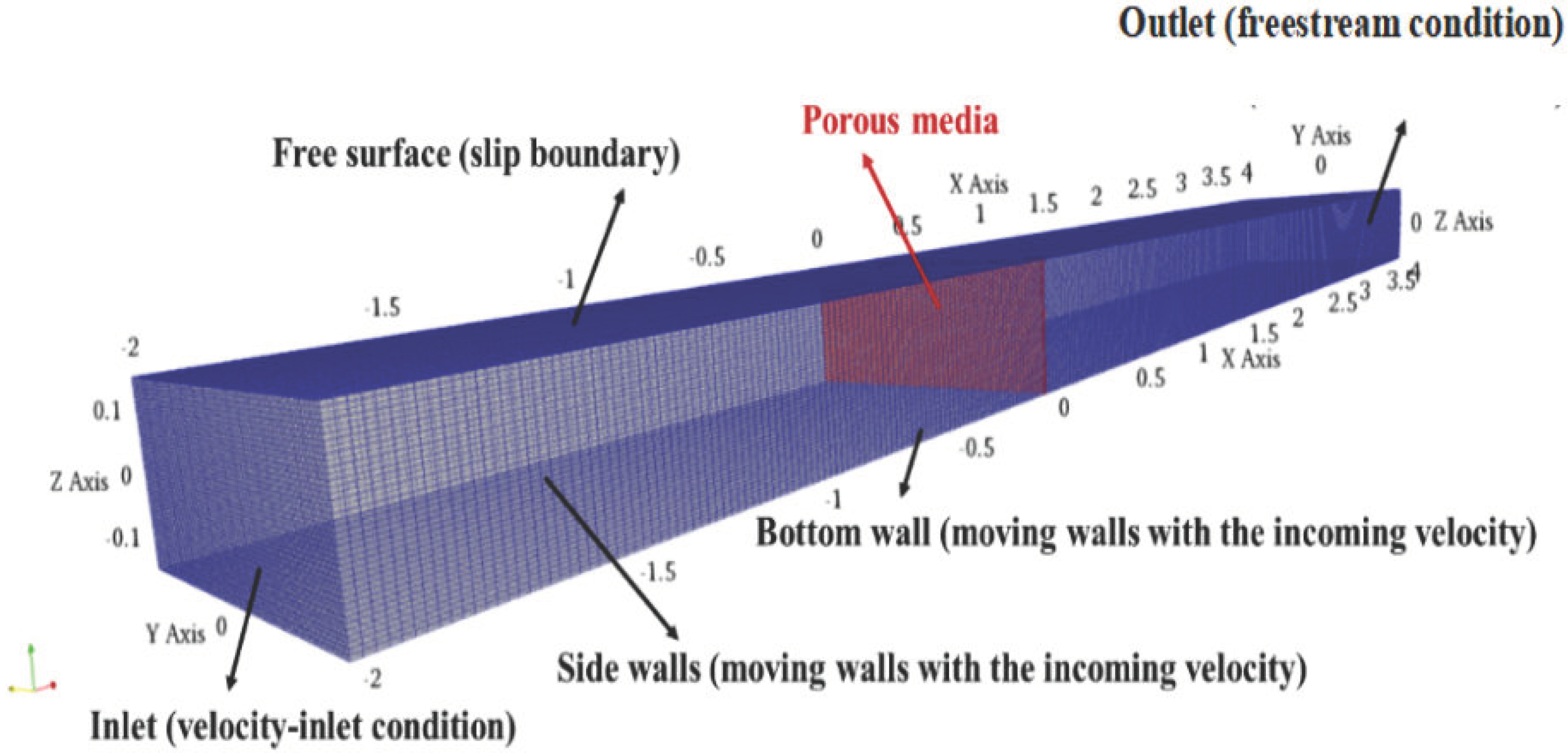
2.3. Mesh Grids and Boundary Conditions

A three-dimensional numerical model domain was set up to represent a rectangular open channel to simulate a fish net panel (porous media) covering the full flow width and depth. A three-dimensional Cartesian coordinate system was adopted with x being the positive direction along the channel, y being perpendicular to the main flow direction on the horizontal plane, and z being the vertical upward direction. The center of the porous media was set the origin (0,0,0) of the coordinate system. Corresponding to the experimental flume configuration [8], the overall numerical domain was 6 m long, 0.8 m wide, and 0.3 m high. Uniform hexahedron cells measuring 2 cm × 1 cm × 0.75 cm were generated in the OpenFOAM mesh generator blockMesh with 9.6 × 10⁵ cells (300 × 80 × 40, Figure 1). Mesh size independence within the numerical simulations was examined by reducing the cell size to 1.5 cm × 0.5 cm × 0.5 cm, and no significant variation on the simulation results was found.
Following Patursson et al. [18], the free surface of the computational domain was specified as a slip boundary condition with zero shear force, and the bottom and side walls were specified as moving walls with the incoming velocity [33]. The upstream boundary was set as the velocity-inlet condition, while the downstream boundary was set as the freestream condition [20]. The initial velocity was set to U0 (see Table 1) throughout the domain, and the turbulent kinetic energy k and turbulence dissipation rate ε were calculated following Rodi [34]:
I = 0.16 R e 1 8 ,     k = 1.5 U 2 I 2 ,     ε = C μ 3 4 k 1.5 / l
where R e is the Reynolds number calculated by the hydraulic diameter of the flume, I is the turbulence intensity, U is the mean flow velocity, and l = 0.07 D H is the turbulence length scale calculated by the hydraulic diameter of the flume D H [19,20].

2.4. Numerical Solver

In this study the numerical simulation was conducted with OpenFOAM v6 [33], employing the finite volume method (FVM) to discretize the governing Navier–Stokes equations. In order to simulate the velocity field and concentration field simultaneously, a user-defined solver passiveScalarPisoFoam was developed by adding the passive scalar transport equation in scalarTransportantFoam solver to the built-in pisoFoam solver [33]. The PISO algorithm [35] was employed as the main velocity and pressure solver. Convective and diffusive terms in the momentum equations were approximated by the second-order central differencing scheme. The convective term in the scalar transport equation was discretized by the MUSCL scheme [36], and the diffusive term in the equation was approximated by a second-order central differencing scheme. The time integration was carried out by a second-order backward scheme. The time step was set as 0.01 s or 0.02 s so that the resultant Courant number was assured to be below 0.5. The total simulation duration was adjusted to ensure the flow had reached a steady state, and only the steady-state simulation results were used in the subsequent analysis.

3. Model Calibration and Validation

The experimental tests of flow and scalar transport for a steady current passing through a rigid fishing net panel, as originally reported in Zeng et al. [8], were used to calibrate and validate the numerical model. The porous media coefficient C n and the turbulent Schmidt number S c t were calibrated by simulating the two calibration cases (runs C1 and C2 in this study, Table 1), with the calibrated model subsequently validated against another test case (run C3, Table 1). We then applied the validated model to simulate five additional test cases (runs S1–S5, Table 1) with three different incoming velocities (i.e., U0 = 0.1 m/s, 0.25 m/s, and 0.5 m/s) and three different net solidities (i.e., S = 0.15, 0.25, 0.35). This extends our understanding of the specific parametric influences on the net panel wakes generated downstream of the net panels. The net solidity S, defined as the ratio of the projected area of the net panel to the total area enclosed by the panel, was used as the primary dimensionless parameter representing the geometric properties of the rigid net panels. For a knotless square net, the solidity S was calculated as S = 2 d / M d / M 2 (where d is the diameter of the net twine (steel rods) and M is the mesh size) [25,37,38]. The mesh size M was set as 20 mm following the experiments, and the details of the experimental test conditions are reported in Zeng et al. [8].
The time-averaged velocity and concentration fields downstream of the modelled net panel for the calibration case C1 are shown in Figure 2a,b. In Figure 2a, water flows through the porous media (located at x/M = 0), resulting in an initial local decrease in velocity followed by a gradual recovery to the incoming velocity. The simulation results are largely consistent with the experimental counterpart (run X2, Figure 2c,d) [8], except the initial periodic peaks and troughs in velocity measurements immediately downstream of the net panel due to the local flow blockage resulting from the netting structure that is eliminated by the numerical treatment of a homogeneous porous media. As such, we neglect the area in the immediate vicinity of the nets (x/M = 0–4) in our subsequent analyses. The simulated spreading of the scalar plume is also slightly wider than the experimental counterpart. However, as demonstrated in the calibration and validation results in the following, the agreement in concentration decay is fairly satisfactory.
In addition, the variations in the mean streamwise velocity along the x direction for cases C1 and C2 are compared with the numerical results and the corresponding experimental data, i.e., runs X2 and X3, respectively, from Zeng et al. [8] in Figure 3a. The simulated mean concentration along the x direction for these calibration cases are also compared with the corresponding experimental data in Figure 3b. Here, the mean streamwise velocity U and the mean concentration C are normalized by the incoming velocity U0 and the inlet concentration C0, respectively. The downstream distance x is normalized by the mesh size M. As shown in Figure 3, the simulated results for U/U0 (R2 = 0.99, RMSE = 1.4%, NRMSE = 1.4% for both case C1 and C2) and C0/C (R2 = 0. 94 and 0.95, RMSE = 10.6% and 12.1%, NRMSE = 6.1% and 6.8% for case C1 and C2, respectively) compare well with the experimental results over the range of x/M values considered (i.e., x/M = 4–10).
Based on the calibration, the thickness of the porous media is determined to be 40 mm and the porous media coefficients C n are determined as 44.7 m−1 and 49.2 m−1 for calibration cases C1 and C2. The turbulent Schmidt number S c t is determined as 1.075, which falls in the range of the reported values for experiments and numerical simulations of scalar transport in open channel flows [39]. In addition, through their conversion relationship defined by Equation (14), we compared the calibrated values of the porous media coefficient C n and empirical formulas of the drag coefficient C d summarized by Zhan et al. [40]. As shown in Figure 4, the calibrated values are in good agreement with the empirical formulae proposed by Zhan et al. [40] amongst the various empirical formulas (e.g., Milne [41]):
C d = 1 + c 1 U 0 + c 2 S + c 3 S 2
where S is the net solidity, c 1 = 0.137 m / s , c 2 = 1.002 , c 3 = 2.230 .
We used the above formula to calculate the porous media coefficient of the validation case (run C3), i.e., C n = 48.5 m1. In Figure 5, we then compared simulated mean normalized streamwise velocities U/U0 (R2 = 0.99) and concentrations C0/C (R2 = 0.92) for validation case C3 with the corresponding experimental data (i.e., run X4, Zeng et al. [8]), and the agreement in both cases is satisfactory.

4. Results and Discussion

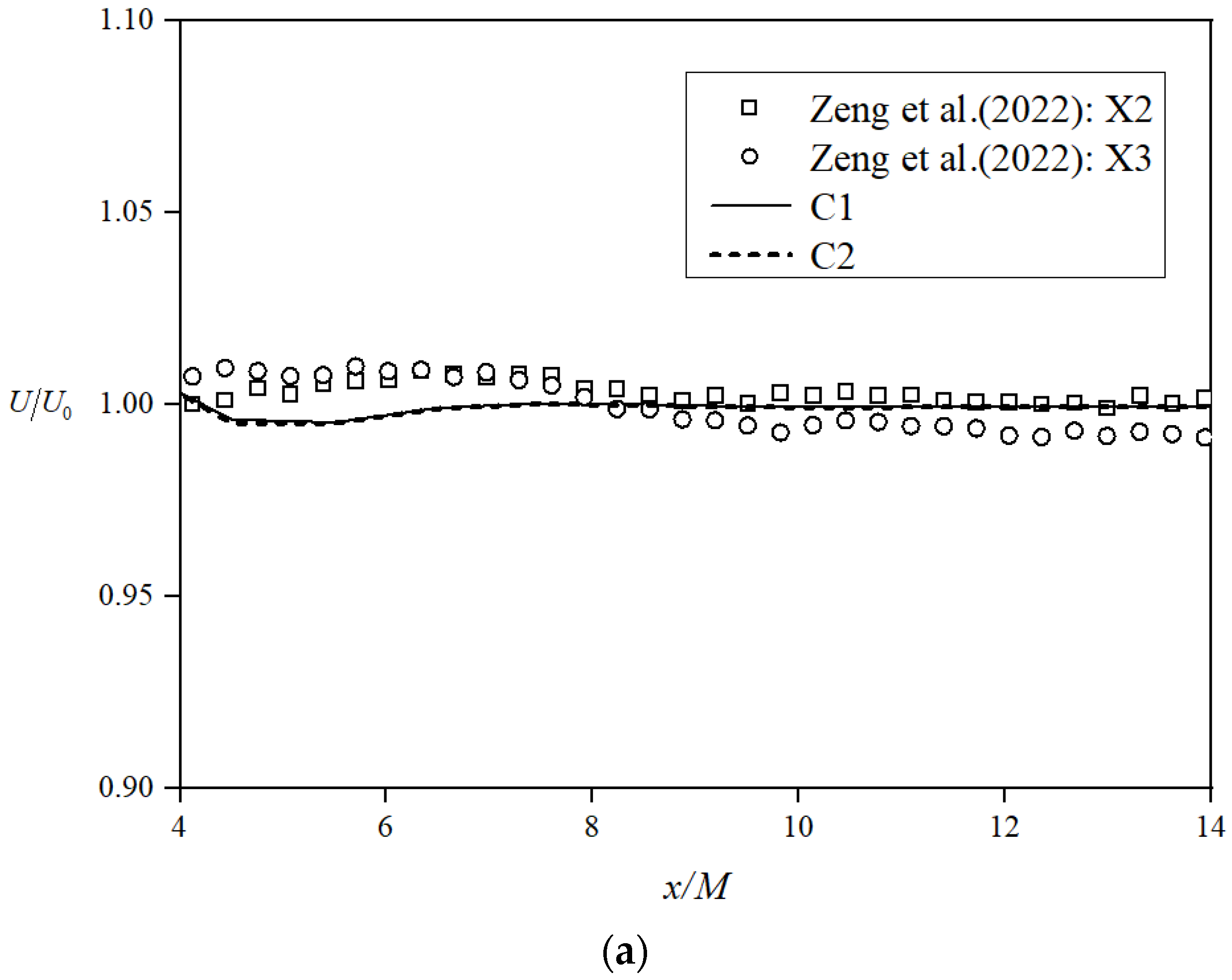
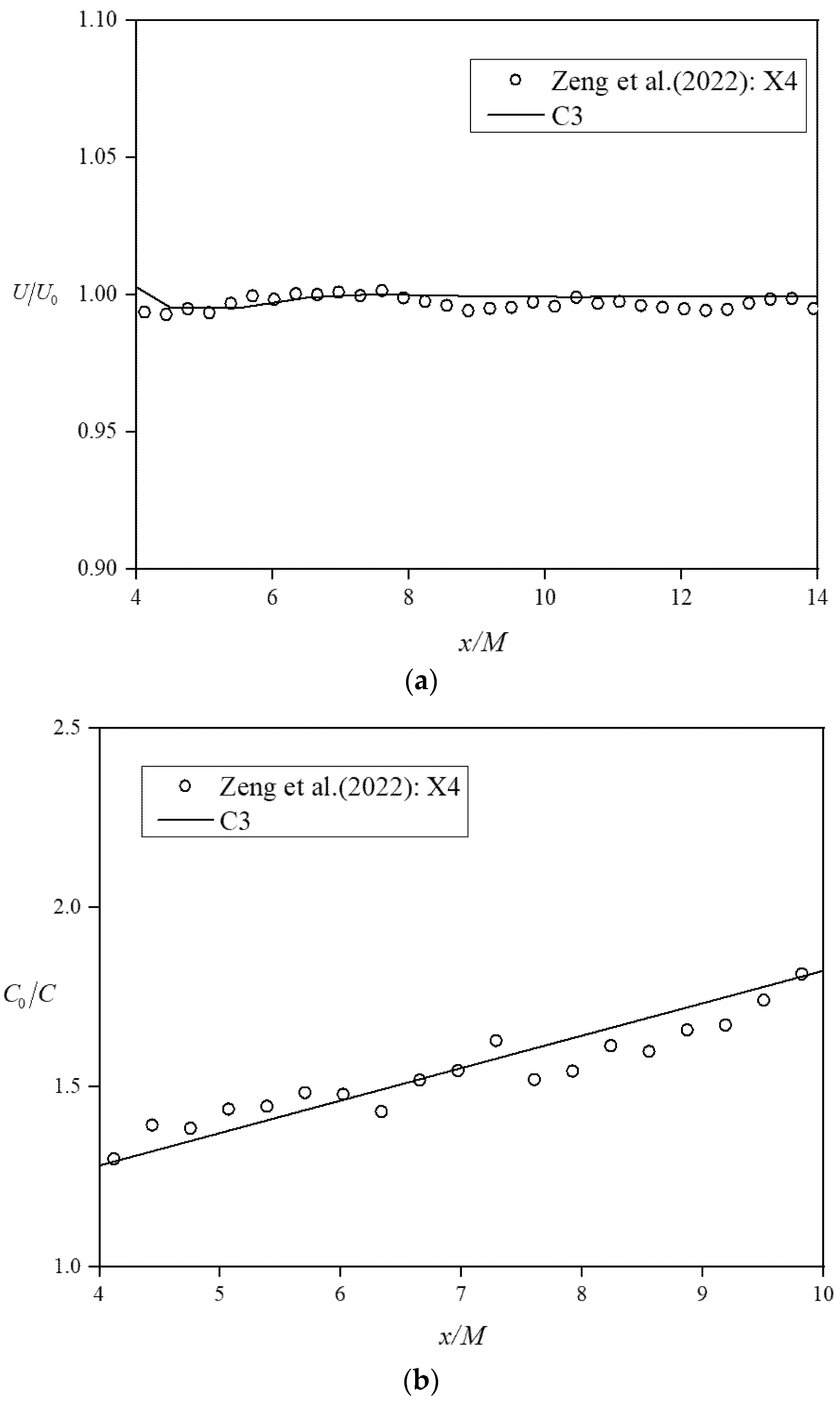
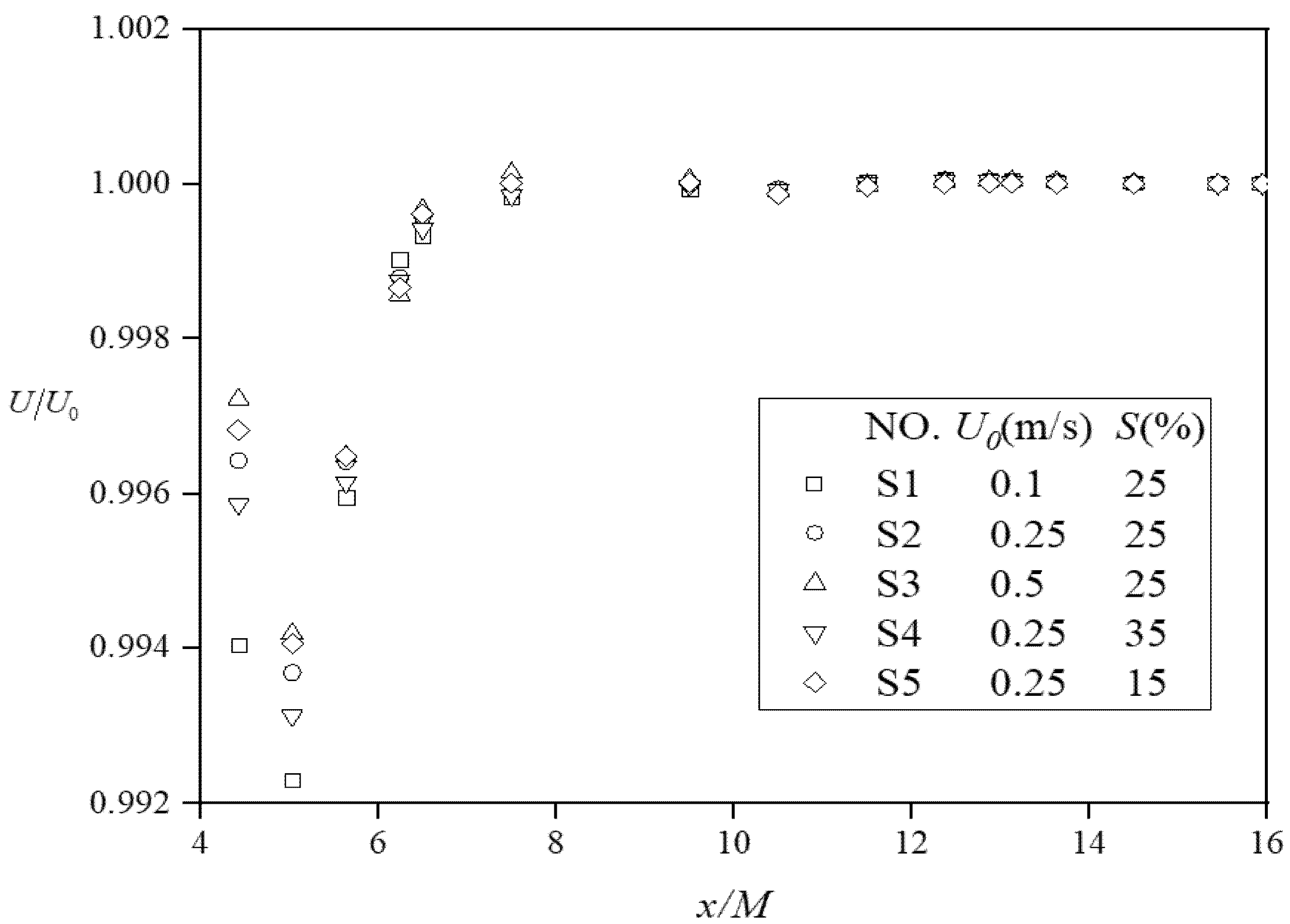
4.1. Velocity Reduction and Recovery

The flow velocity reduction factors U/U0 in the x direction for the five scenario simulation cases are shown in Figure 6. We use the flow velocity reduction factor U/U0 to measure the effects of flow blockage from the net structure, which is also widely used in the literature [8,23]. As shown in Figure 6, the recovery of the flow velocity downstream of the net panel (i.e., to U/U0 = 1) is achieved for all cases at approximately x/M = 14, which is consistent with the results of Zeng et al. [8]. Among the parametric cases with constant incoming velocity but varying net solidities, (i.e., runs S2, S4, and S5, Table 1), the flow velocity reduction tends to be weaker as the net solidity decreases, confirming that low net solidity of a fishing net panel leads to less blockage effect in the downstream flow fields, as expected. Similar trends have been reported from previous studies [23,24,42,43], while Tu et al. [24] also reported that low net solidity leads to reduced water blockage, by comparing the distance from the net to the downstream position where velocity behind the central twine and the adjacent mesh becomes uniform for nets with different net solidities. In contrast, for the scenario cases with constant net solidity but varying incoming velocities (i.e., runs S1, S2, and S3, Table 1), the flow velocity reduction tends to be weaker as the incoming velocity increases, consistent with Zeng et al. [8]. Notably, Yao et al. [43] reported that lower-flow Reynolds numbers, associated with lower incoming velocities, caused larger drag coefficients, such that the flow velocity reduction across the net panel tended to be stronger. Therefore, the flow velocity reduction tends to increase with increasing net solidity and decreasing incoming velocity in the near field, with the latter appearing to affect the velocity reduction more significantly than the former within our parametric range of variation. Similar findings have also been reported by Shao et al. [7] for flow reduction through flexible net panels.

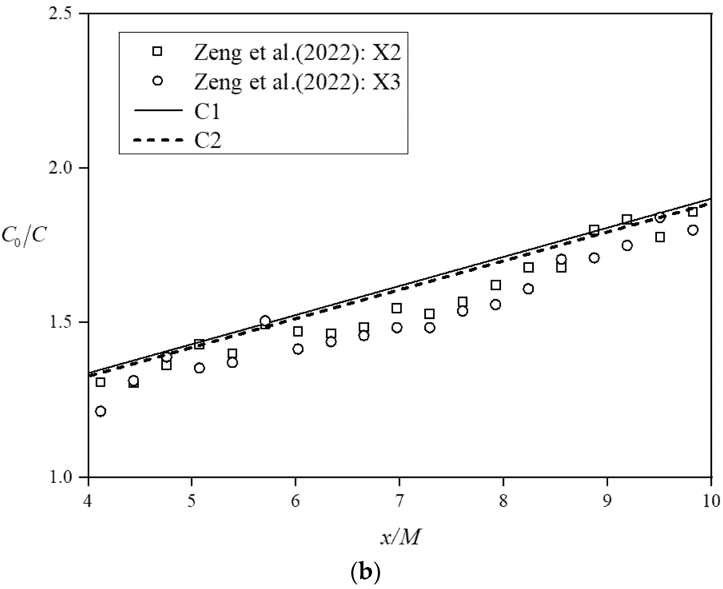
4.2. Concentration Decay

The longitudinal profiles of the inverse of the normalized mean concentration C0/C along the plume centerline for the various scenario cases are shown in Figure 7. Lemoine et al. [17] studied the tracer transport process from a point source into grid turbulence, and reported that the inverse of the concentration (1/C) grows linearly with the downstream distance x/M. In this context, our results confirmed the steady growth of the concentration decay between x/M = 4 and x/M = ~50.
Furthermore, among the cases with constant incoming velocity but varying net solidities (i.e., S2, S4, and S5, Table 1), there is no discernible differences in the scalar concentration decay in the far field. In contrast, for cases with constant net solidity but varying incoming velocities (i.e., S1, S2, and S3, Table 1), it is clearly shown that the scalar concentration decay tends to be stronger in the far field as the incoming velocity decreases.

4.3. Plume Spreading

Figure 8 shows the normalized lateral profiles of the scalar concentration at different downstream locations for Case S2 (Table 1), which exhibits self-similar Gaussian distributions of the form [8]:
C x , y = C c x e x p y 2 σ y 2
where σ y is the standard deviation in the transverse direction representing the spreading width of the scalar plume, C x , y is the time-averaged concentration at location x , y , and C c x is the concentration at the plume centerline. This is consistent with the experimental findings of Lemoine et al. [17] (Figure 4) and Zeng et al. [8] (Figure 6a), that the lateral concentration profile appears to follow a Gaussian distribution even at near-field locations, much closer to the net (grid) where the wake-flow field is strongly inhomogeneous.
Figure 9 shows the variation of the non-dimensional plume spreading width σ y with downstream distance for the various cases. The plume spreading width grows in the streamwise direction from x/M = ~4 to x/M = ~50, consistent with the experimental results that show the plume spreading width grows linearly on a logarithmic scale for x/M > ~4 [8]. There is also a significant change of slope at x/M = ~13, which is again consistent with the findings of [15] who indicated that the slopes of the plume growth in the near and far field are different. As shown in Figure 9, the slope is lower than 0.5 (i.e., σ y x / M ) in the near field but changes to ~0.5 when transitioning to the far field, indicative of the transition of the plume development from the turbulent-convective regime to the turbulent-diffusive regime [8].
Among the cases with constant incoming velocity but varying net solidities (i.e., S2, S4, and S5, Table 1), the plume growth trajectories for different net solidities appear to collapse with each other, consistent with their concentration decay results. In contrast, for the cases with constant net solidity but varying incoming velocities (i.e., S1, S2, and S3, Table 1), the plume spreading width tends to be larger as the incoming velocity decreases, presumably leading to the enhanced scalar concentration decay observed with reduced incoming velocity (Figure 7). According to Taylor’s diffusion theory, when the plume development enters the turbulent-diffusive regime, the plume spreading width follows:
d σ y 2 d k = 2 D U  
where D denotes the turbulent diffusivity or Taylor diffusivity. As the plume development transitions into the turbulent-diffusive regime from near field to far field, it should follow the square-root growth with downstream distance x and be inversely correlated with the mean velocity. Therefore, with decreasing incoming velocity, the plume grows wider towards downstream, and the scalar concentration decay becomes stronger.
Nutrients and contaminants contained in the surrounding waters around the fish cages will be carried by the current and enter the cages through the cage sidewall nets. Likewise, uneaten feeds, faces, chemical treatments, and other wastes generated through aquaculture practice inside the cages will be discharged into the wider aquatic environment through the cage nets [4]. Therefore, depending on the source of the substance and the direction of the current, the source location relative to the net panel can vary from upstream to downstream. To explore the potential effects of the source location on plume development, Figure 10 shows the non-dimensional plume spreading width σ y with three different source locations, namely, x’/M = −10, x’/M = 0, and x’/M =10 for S2, where x’ is the source location relative to the fishing net panel (the origin of the coordinate system), and Δx/M is the non-dimensional streamwise distance from the source. As shown in Figure 10, the plume development appears to be independent of source location, which is presumably due to the assumption of the RANS model that disregards the evolving turbulence field at varying distances from the net. Notably, Warhaft [44] studied the effect of turbulence intensity at the source by changing its downstream location with respect to the grid, finding that the mean profile spread more rapidly as the grid position got closer to the line source (i.e., where the turbulence intensity is greater). Similar findings have also been reported by Rummel et al. [15].

5. Conclusions

A CFD model was developed using OpenFOAM to study the time-averaged flow field and scalar transport processes through a fishing net panel with different net solidities and incoming velocities. The main findings of this study are summarized as follows:
(1)
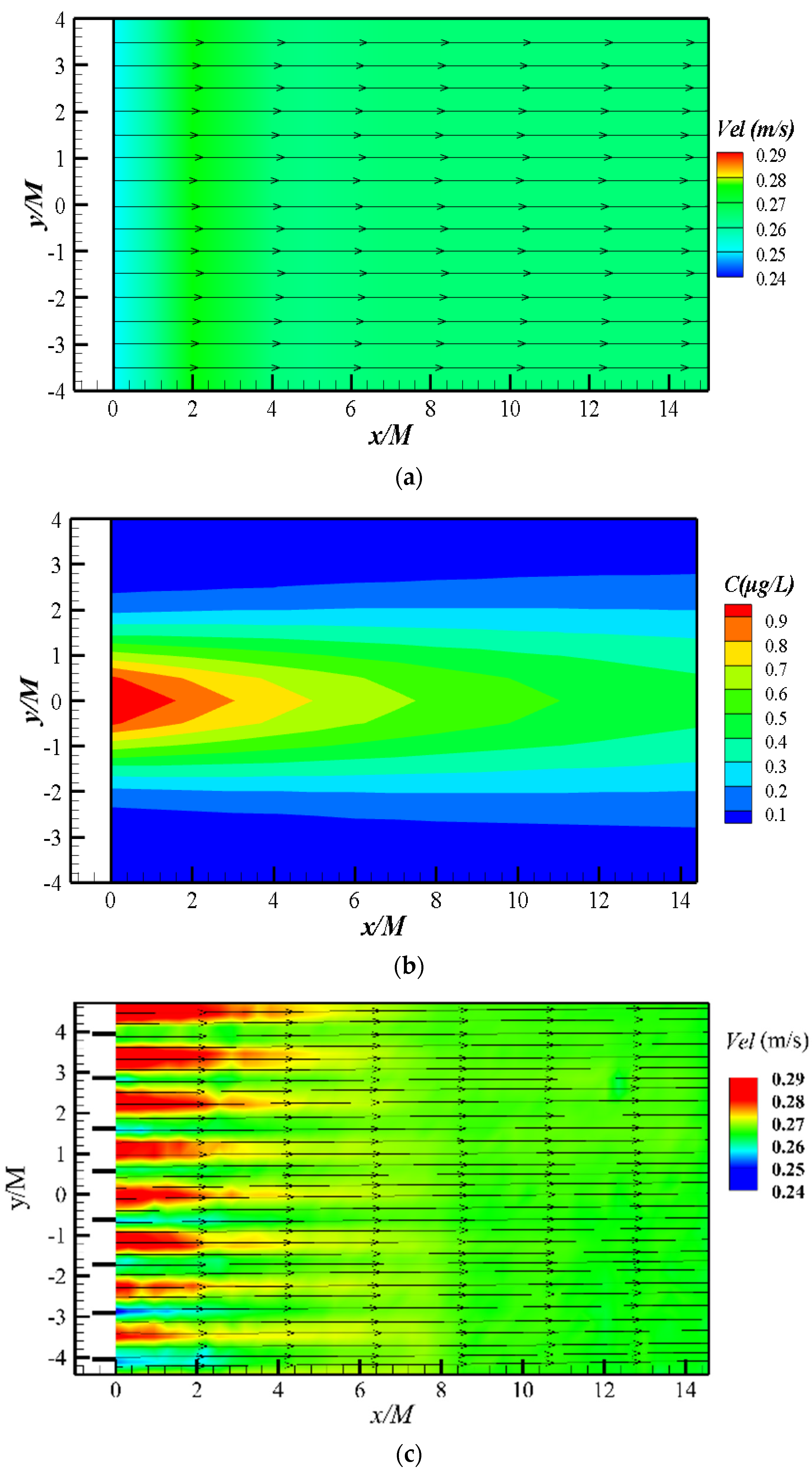
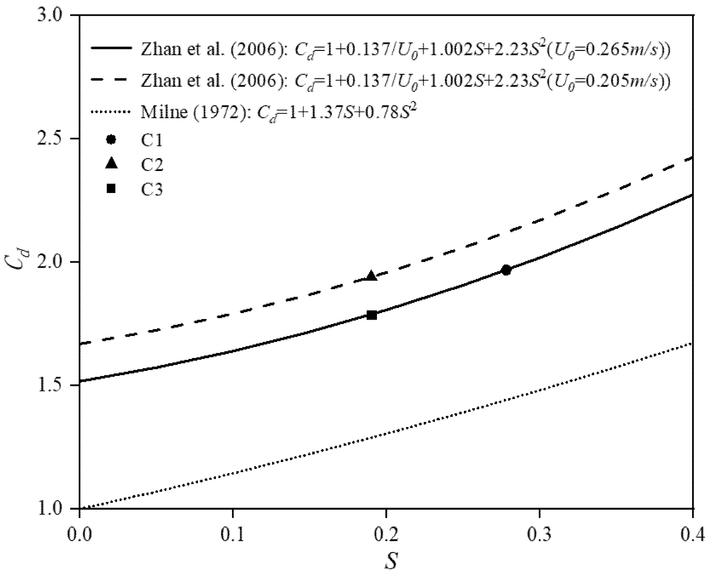
The time−averaged velocity and concentration fields could be reasonably reproduced by a standard k-ε model implemented in OpenFOAM, in which the fishing net panel was treated as a porous media. The numerical model was calibrated and validated by experimental data, and the comparisons showed good agreement, indicating that the porous media schematization could reproduce the blocking effect of the net on the flow field, except for the inhomogeneous wake field at the immediate vicinity of the net panel, and the associated mass transport, with satisfactory accuracy.
(2)
Our simulation results showed a clear reduction in time-averaged flow velocity behind the net. At the same time, the complete recovery of velocity was observed within the downstream extent of the numerical simulations (i.e., x/M ~ 14). The flow velocity reduction tends to increase with increasing net solidity and decreasing incoming velocity in the near field. Moreover, the incoming velocity appeared to affect the flow velocity reduction more significantly than the net solidity for the range of variation covered in our study.
(3)
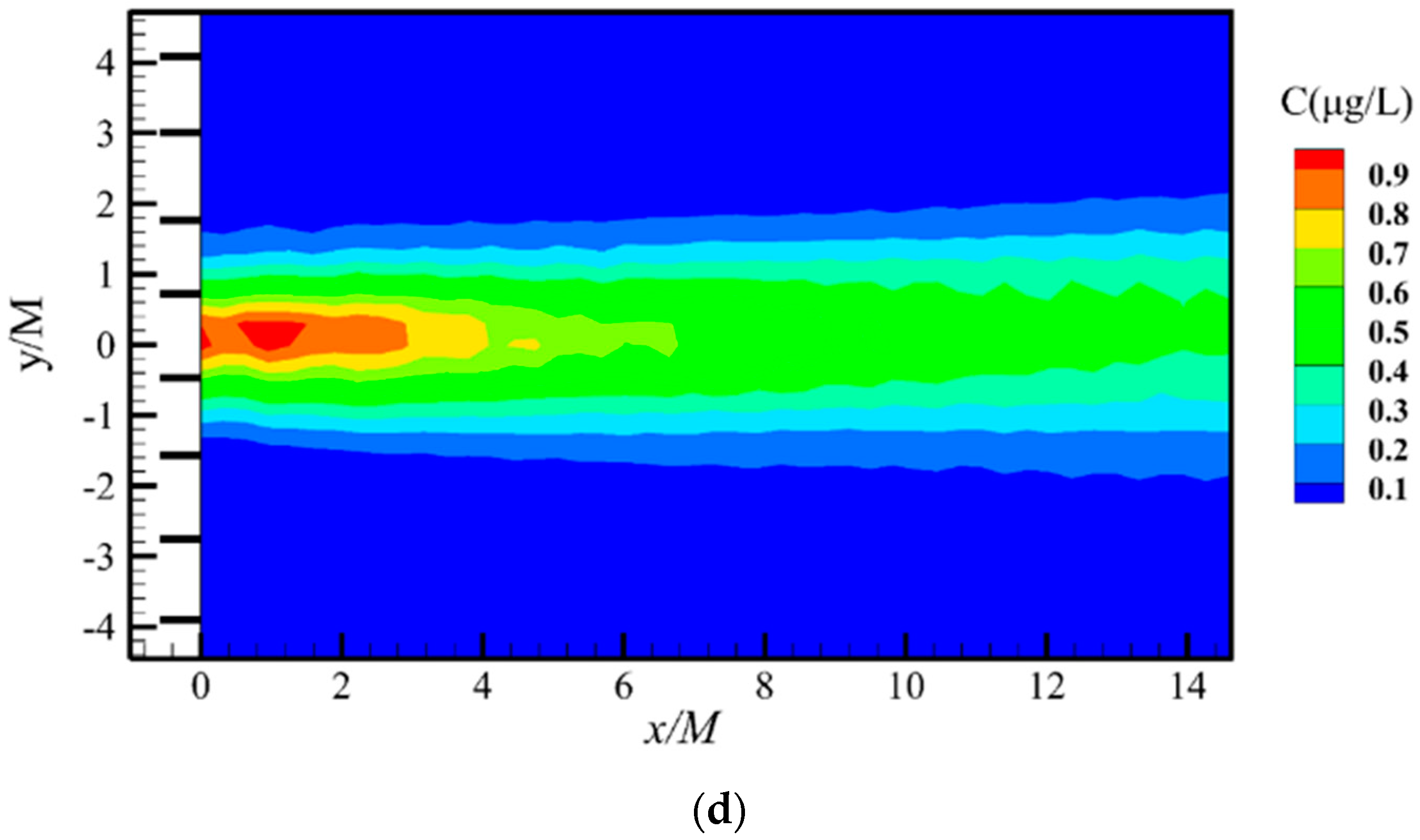
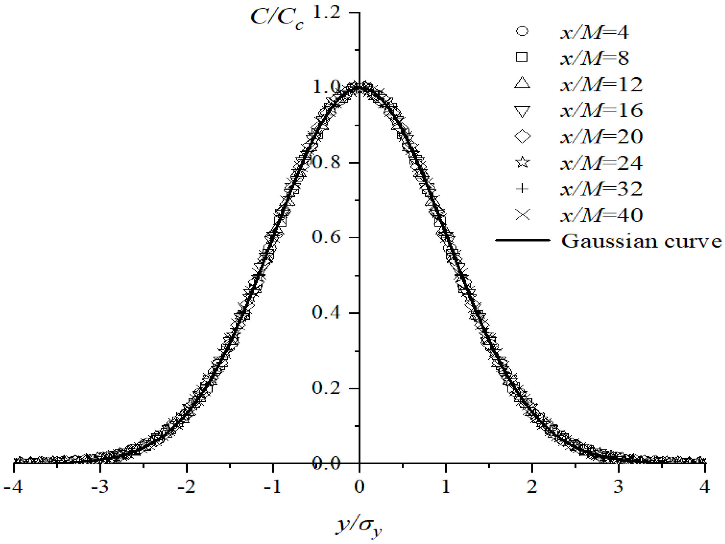
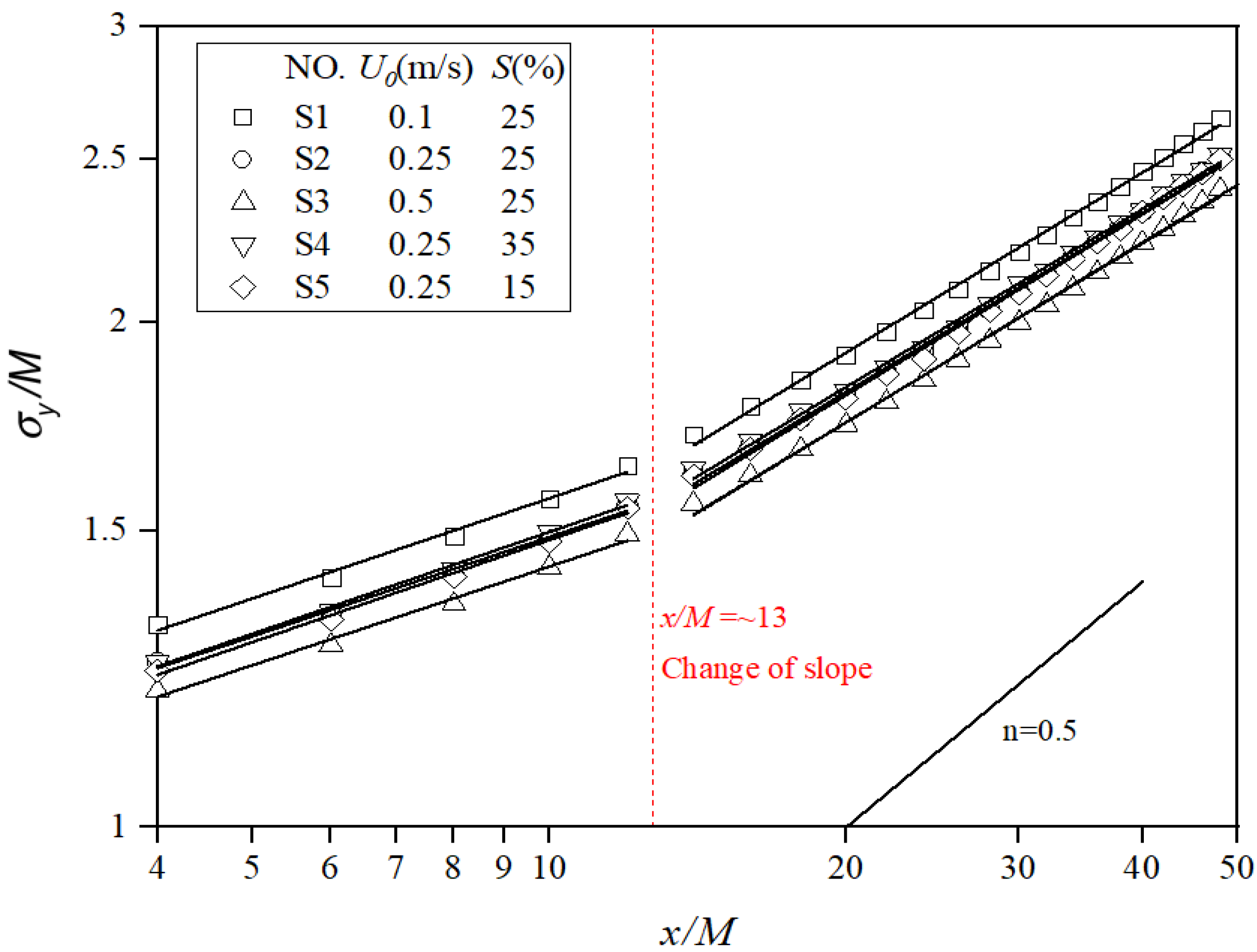
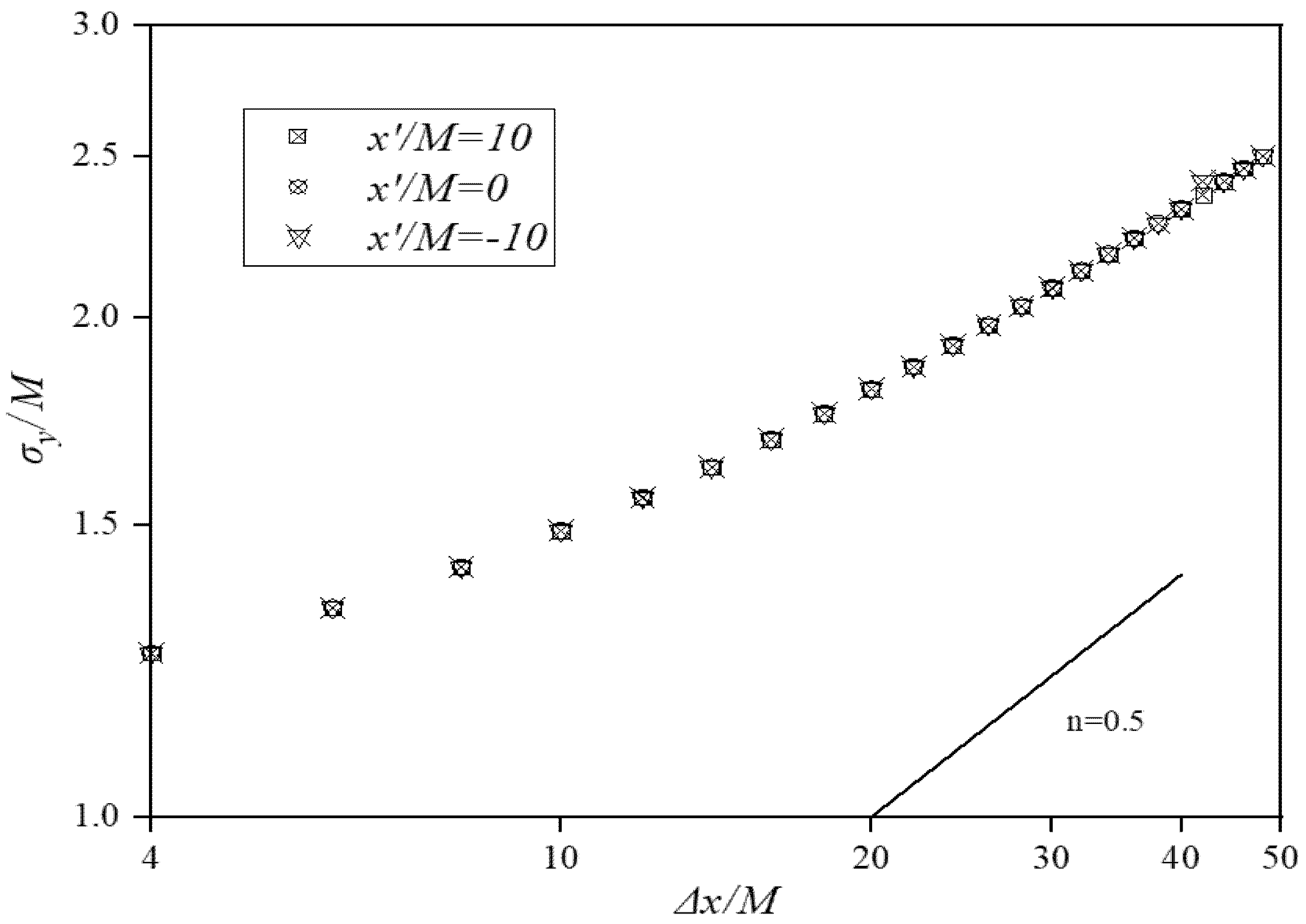
The scalar concentration decay tends to be stronger as the incoming velocity decreases, and the lateral profile of the scalar concentration exhibited self-similarity and followed Gaussian distribution, in agreement with experimental data. Furthermore, the spreading of plume width is reduced with increasing incoming velocity, but does not seem to be largely affected by the source location relative to the net when adopting the current RANS and porous media modelling approach.
Our study provides the first attempt toward modeling the effects on the scalar concentration field from the fishing net panel using the RANS approach and adopting a porous media model to represent cage net panels. As acknowledged above, future studies incorporating the effects of turbulence can offer a closer look at the effects of source location on plume development, among other aspects of plume behavior. Moreover, modeling the net as a porous media rather than a large number of cylinders connected by knots could not faithfully resolve the inhomogeneous wake field behind the twine and the adjacent mesh hole, and large-eddy simulation (LES) methodology may be considered for such a task in the future as presented by Zenklusen et al. [45].

Supplementary Materials

The following supporting information can be downloaded at: https://www.mdpi.com/article/10.3390/jmse10101511/s1. File S1 needs to unpacked by the professional software firstly. Then the file can be opened as the text and run in the OpenFOAM software.

Author Contributions

Conceptualization, D.S.; methodology, X.Y., X.Z., D.S. and R.-Q.W.; software, X.Y., X.Z. and R.-Q.W.; validation, D.S.; formal analysis, X.Y., X.Z. and D.S.; investigation, X.Y. and D.S.; resources, D.S.; data curation, X.Y. and X.Z.; writing—original draft preparation, X.Y. and X.Z.; writing—review and editing, D.S., C.G., A.C. and R.-Q.W.; visualization, X.Y.; supervision, D.S., C.G., A.C. and R.-Q.W.; project administration, D.S.; funding acquisition, D.S., C.G., A.C. and R.-Q.W. All authors have read and agreed to the published version of the manuscript.

Funding

This work was supported by the National Natural Science Foundation of China (Grant No. 51779012 and 51811530316), the National Key Research and Development Program of China (Grant No. 2018YFC1406404), and Interdisciplinary Research Funds of Beijing Normal University. The authors (DS, RQW and AC) are also grateful for financial support provided by The Royal Society through an International Exchange Cost Share (China) 2017 Grant (Grant No. IEC\NSFC\170104) which facilitated bilateral research visits between Beijing Normal University and the University of Dundee. Financial support for C. Gualtieri from the State Administration of Foreign Experts Affairs of China is also gratefully acknowledged.

Institutional Review Board Statement

Not applicable.

Informed Consent Statement

Not applicable.

Data Availability Statement

All data necessary to carry out the work in this paper are included in the figures and tables or are available in the cited references.

Conflicts of Interest

The authors declare no conflict of interest.

References

  1. Weiss, C.V.C.; Ondiviela, B.; Guanche, R.; Castellanos, O.F.; Juanes, J.A. A global integrated analysis of open sea fish farming opportunities. Aquaculture 2018, 497, 234–245. [Google Scholar] [CrossRef]
  2. Klebert, P.; Lader, P.; Gansel, L.; Oppedal, F. Hydrodynamic interactions on net panel and aquaculture fish cages: A review. Ocean Eng. 2013, 58, 260–274. [Google Scholar] [CrossRef]
  3. Venayagamoorthy, S.K.; Ku, H.; Fringer, O.B.; Chiu, A.; Naylor, R.L.; Koseff, J.R. Numerical modeling of aquaculture dissolved waste transport in a coastal embayment. Environ. Fluid Mech. 2011, 11, 329–352. [Google Scholar] [CrossRef]
  4. Wang, X.; Cuthbertson, A.; Gualtieri, C.; Shao, D. A review on mariculture effluent: Characterization and management Tools. Water 2020, 12, 2991. [Google Scholar] [CrossRef]
  5. Price, C.; Black, K.D.; Hargrave, B.T.; Morris, J.A., Jr. Marine cage culture and the environment: Effects on water quality and primary production. Aquac. Environ. Interact. 2015, 6, 151–174. [Google Scholar] [CrossRef] [Green Version]
  6. Suzuki, K.; Takagi, T.; Shimizu, T.; Hiraishi, T.; Yamamoto, K.; Nashimoto, K. Validity and visualization of a numerical model used to determine dynamic configurations of fishing nets. Fish. Sci. 2003, 69, 695–705. [Google Scholar] [CrossRef] [Green Version]
  7. Shao, D.; Huang, L.; Wang, R.Q.; Gualtieri, C.; Cuthbertson, A. Flow turbulence characteristics and mass transport in the near-wake region of an aquaculture cage net panel. Water 2021, 13, 294. [Google Scholar] [CrossRef]
  8. Zeng, X.; Gualtieri, C.; Cuthbertson, A.; Shao, D. Experimental study of flow and mass transport in the near-wake region of a rigid planar metal net panel. Aquac. Eng. 2022, 98, 102267. [Google Scholar] [CrossRef]
  9. Lee, C.W.; Kim, Y.B.; Lee, G.H.; Choe, M.Y.; Lee, M.K.; Koo, K.Y. Dynamic simulation of a fish cage system subjected to currents and waves. Ocean Eng. 2008, 35, 1521–1532. [Google Scholar] [CrossRef]
  10. Cha, B.J.; Kim, H.Y.; Bae, J.H.; Yang, Y.S.; Kim, D.H. Analysis of the hydrodynamic characteristics of chain-link woven copper alloy nets for fish cages. Aquac. Eng. 2013, 56, 79–85. [Google Scholar] [CrossRef]
  11. Bi, C.W.; Zhao, Y.P.; Dong, G.H.; Xu, T.J.; Gui, F.K. Experimental investigation of the reduction in flow velocity downstream from a fishing net. Aquac. Eng. 2013, 57, 71–81. [Google Scholar] [CrossRef]
  12. Cuthbertson, A.J.S.; Malcangio, D.; A Davies, P.; Mossa, M. The influence of a localised region of turbulence on the structural development of a turbulent, round, buoyant jet. Fluid Dyn. Res. 2006, 38, 683–698. [Google Scholar] [CrossRef]
  13. Nakamura, I.; Sakai, Y.; Miyata, A. Diffusion of matter by a non-buoyant plume in grid-generated turbulence. J. Fluid Mech. 1987, 178, 379–408. [Google Scholar] [CrossRef]
  14. Nedić, J.; Tavoularis, S. Measurements of passive scalar diffusion downstream of regular and fractal grids. J. Fluid Mech. 2016, 800, 358–386. [Google Scholar] [CrossRef]
  15. Rummel, A.C.; Socolofsky, S.A.; Carmer, C.F.V.; Jirka, G.H. Enhanced diffusion from a continuous point source in shallow free-surface flow with grid turbulence. Phys. Fluids 2005, 17, 075105. [Google Scholar] [CrossRef]
  16. Lemoine, F.; Antoine, Y.; Wolff, M.; Lebouche, M. Mass transfer properties in a grid generated turbulent flow: Some experimental investigations about the concept of turbulent diffusivity. Int. J. Heat Mass Transf. 1998, 41, 2287–2295. [Google Scholar] [CrossRef]
  17. Lemoine, F.; Wolff, M.; Lebouché, M. Experimental investigation of mass transfer in a grid-generated turbulent flow using combined optical methods. Int. J. Heat Mass Transf. 1997, 40, 3255–3266. [Google Scholar] [CrossRef]
  18. Patursson, Ø.; Swift, M.R.; Tsukrov, I.; Simonsen, K.; Baldwin, K.; Fredriksson, D.W.; Celikkol, B. Development of a porous media model with application to flow through and around a net panel. Ocean Eng. 2010, 37, 314–324. [Google Scholar] [CrossRef]
  19. Zhao, Y.P.; Bi, C.W.; Dong, G.H.; Gui, F.K.; Cui, Y.; Guan, C.T.; Xu, T.J. Numerical simulation of the flow around fishing plane nets using the porous media model. Ocean Eng. 2013, 62, 25–37. [Google Scholar] [CrossRef]
  20. Bi, C.W.; Zhao, Y.P.; Dong, G.H.; Xu, T.J.; Gui, F.K. Numerical simulation of the interaction between flow and flexible nets. J. Fluids Struct. 2014, 45, 180–201. [Google Scholar] [CrossRef]
  21. Tang, H.; Bruno Thierry, N.N.; Pandong, A.N.; Sun, Q.; Xu, L.; Hu, F.; Zou, B. Hydrodynamic and turbulence flow characteristics of fishing nettings made of three twine materials at small attack angles and low Reynolds numbers. Ocean Eng. 2022, 249, 110964. [Google Scholar] [CrossRef]
  22. Santo, H. On the application of current blockage model to steady drag force on fish net. Aquac. Eng. 2022, 97, 102226. [Google Scholar] [CrossRef]
  23. Løland, G. Current forces on, and water flow through and around, floating fish farms. Aquac. Int. 1993, 1, 72–89. [Google Scholar] [CrossRef]
  24. Tu, G.; Liu, H.; Ru, Z.; Shao, D.; Yang, W.; Sun, T.; Wang, H.; Gao, Y. Numerical analysis of the flows around fishing plane nets using the lattice Boltzmann method. Ocean Eng. 2020, 214, 107623. [Google Scholar] [CrossRef]
  25. Batchelor, G.K. The Theory of Homogeneous Turbulence; Cambridge University Press: Cambridge, UK, 1953. [Google Scholar]
  26. Gorle, J.; Terjesen, B.; Summerfelt, S. Influence of inlet and outlet placement on the hydrodynamics of culture tanks for Atlantic salmon. Int. J. Mech. Sci. 2020, 188, 105944. [Google Scholar] [CrossRef]
  27. Pope, S.B. Turbulent Flows; Cambridge University Press: Cambridge, UK, 2000; p. 771. [Google Scholar]
  28. Patursson, Ø.E.; Swift, M.R.; Tsukrov, I.; Baldwin, K.; Simonsen, K. Modeling flow through and around a net panel using computational fluid dynamics. In Proceedings of the OCEANS, Boston, MA, USA, 18–21 September 2006; pp. 1–5. [Google Scholar]
  29. Launder, B.E.; Spalding, D.B. The numerical computation of turbulent flows. Comput. Methods Appl. Mech. Eng. 1974, 3, 269–289. [Google Scholar] [CrossRef]
  30. Burcharth, H.F.; Andersen, O.H. On the one-dimensional steady and unsteady porous flow equations. Coast. Eng. 1995, 24, 233–257. [Google Scholar] [CrossRef]
  31. Chen, H.; Christensen, E.D. Investigations on the porous resistance coefficients for fishing net structures. J. Fluids Struct. 2016, 65, 76–107. [Google Scholar] [CrossRef] [Green Version]
  32. Morison, J.R.; Johnson, J.W.; O’Brien, M.P.; Schaaf, S.A. The forces exerted by surface waves on piles. Pet. Trans. Am. Inst. Min. Eng. 1950, 189, 149–154. [Google Scholar] [CrossRef]
  33. OpenCFD. OpenFOAM: The Open Source CFD Toolbos Programmer’s Guide; OpenCFD Ltd.: Bracknell, UK, 2018. [Google Scholar]
  34. Rodi, W. Turbulence Models and Their Application in Hydraulics—A State of the Art Review, 3rd ed.; IAHR Monograph: Delft, The Netherlands, 1993; p. 104. [Google Scholar]
  35. Issa, R. Solution of the implicit discretized fluid flow equations by operator splitting. J. Comput. Phys. 1986, 62, 40–65. [Google Scholar] [CrossRef]
  36. Van Leer, B. Toward the ultimate conservative difference scheme. Part IV: A new approach to numerical convection. J. Comput. Phys. 1979, 23, 276–299. [Google Scholar] [CrossRef]
  37. Aarsnes, J.V.; Rudi, H.; Løland, G. Current Forces on Cage, Net Deflection; Thomas Telford: London, UK, 1990; pp. 137–152. [Google Scholar]
  38. Launder, B.E.; Spalding, D.B. Lectures in Mathematical Model of Turbulence; Academic Press: London, UK, 1972; Available online: https://www.semanticscholar.org/paper/Lectures-in-mathematical-models-of-turbulence-Launder-Spalding/19dad37ff5b1f0ae15b067758ec5a47e8692c840 (accessed on 25 August 2022).
  39. Gualtieri, C.; Angeloudis, A.; Bombardelli, F.; Jha, S.; Stoesser, T. On the Values for the Turbulent Schmidt Number in Environmental Flows. Fluids 2017, 2, 17. [Google Scholar] [CrossRef] [Green Version]
  40. Zhan, J.M.; Jia, X.P.; Li, Y.S.; Sun, M.G.; Guo, G.X.; Hu, Y.Z. Analytical and experimental investigation of drag on nets of fish cages. Aquac. Eng. 2006, 35, 91–101. [Google Scholar] [CrossRef]
  41. Milne, P.H. Fish and Shellfish Farming in Coastal Waters; Fishing News: London, UK, 1972. [Google Scholar]
  42. Cornejo, P.; Sepúlveda, H.H.; Gutiérrez, M.H.; Olivares, G. Numerical studies on the hydrodynamic effects of a salmon farm in an idealized environment. Aquaculture 2014, 430, 195–206. [Google Scholar] [CrossRef]
  43. Yao, Y.; Chen, Y.; Zhou, H.; Yang, H. Numerical modeling of current loads on a net cage considering fluid–structure interaction. J. Fluids Struct. 2016, 62, 350–366. [Google Scholar] [CrossRef]
  44. Warhaft, Z. The interference of thermal fields from line sources in grid turbulence. J. Fluid Mech. 1984, 144, 363–387. [Google Scholar] [CrossRef]
  45. Zenklusen, A.; Kenjereš, S.; Rohr, P. Mixing at high Schmidt number in a complex porous structure. Chem. Eng. Sci. 2016, 150, 74–84. [Google Scholar] [CrossRef]
Figure 1. Computational domain with structured grids and boundary conditions.
Jmse 10 01511 g001
Figure 2. Time-averaged (a) velocity field and (b) concentration field downstream of net on the horizontal center plane for the case C1, and (c) velocity field and (d) concentration field downstream of net on the horizontal center plane for the experimental case X2 in Zeng et al. [8].
Jmse 10 01511 g002aJmse 10 01511 g002b
Figure 3. The comparison of the variation of (a) U/U0 and (b) C0/C with longitudinal distance x/M along the flume centerline [8].
Jmse 10 01511 g003aJmse 10 01511 g003b
Figure 4. The comparison of calibrated values of the porous media coefficient C n and empirical formula for the drag coefficient C d [40,41]. Note that C n = C d λ .
Jmse 10 01511 g004
Figure 5. The comparison of the variation of (a) U/U0 and (b) C0/C with longitudinal distance x/M along the flume centerline [8].
Jmse 10 01511 g005
Figure 6. The flow velocity reduction factor U/U0 at different downstream locations in the simulation cases.
Jmse 10 01511 g006
Figure 7. The scalar concentration decay C0/C at different downstream locations.
Jmse 10 01511 g007
Figure 8. Lateral profiles of the normalized time-averaged concentration C/Cc at different downstream locations for S2.
Jmse 10 01511 g008
Figure 9. Evolution of the plume spreading width σ y with downstream distance.
Jmse 10 01511 g009
Figure 10. The downstream evolution of the plume spreads at different source locations for S2.
Jmse 10 01511 g010
Table 1. Parameters of OpenFOAM simulations.
No.Incoming Velocity
U0 (m/s)
Turbulent Kinetic Energy
k (m2/s2)
Turbulence Dissipation Rate ε (m2/s3)Net Solidity
S (%)
Porous Resistance Coefficient Cn (m−1)Time Step
Δt
Simulation Time T (s)
C10.2651.31 × 10−45.1 × 10−619.044.70.0240
C20.2651.31 × 10−45.1 × 10−627.849.20.0240
C30.2058.33 × 10−52.6 × 10−619.048.50.0240
S10.12.37 × 10−53.95 × 10−725.0690.0260
S20.251.18 × 10−44.38 × 10−625.048.40.0240
S30.53.97 × 10−42.7 × 10−525.041.60.0130
S40.251.18 × 10−44.38 × 10−635.054.30.0240
S50.251.18 × 10−44.38 × 10−615.043.70.0240
Publisher’s Note: MDPI stays neutral with regard to jurisdictional claims in published maps and institutional affiliations.

