Numerical Investigation of Flow around Two Tandem Cylinders in the Upper Transition Reynolds Number Regime Using Modal Analysis

Abstract

Flow around two tandem cylinders at Re = 3.6 × 10⁶ for different center-to-center spacing ratio ($L/D$) is investigated numerically using two-dimensional (2D) Unsteady Reynolds-Averaged Navier–Stokes (URANS) equations combined with a standard $k-\omega \mathrm{SST}$ turbulence model. The instantaneous flow structures around the cylinders, hydrodynamic forces on the cylinders and Strouhal number $\left(St\right)$ are analyzed and discussed. Dynamic Mode Decomposition (DMD) is used to extract the spatiotemporal information of the coherent flow structures in the wake regions behind the upstream (UC) and downstream (DC) cylinders. A sparsity-promoted algorithm is implemented to select the dominant modes which contribute the most to the dynamics of the system. Based on the dominant modes, a reduced-order representation of the flows is built. A comparison of the lift and drag force–time histories, obtained by simulation results and the reduced-order representations, shows a high capability of the latter to reproduce the surrounding flow and hydrodynamic properties of the tandem cylinders at the high Reynolds number.

1. Introduction

Flow around tandem cylinders is of industrial and academic interest. In the field of offshore engineering, marine risers and subsea pipelines are usually subjected to a high Reynolds number flow in the order of ${10}^6$ to ${10}^7$ as reported by Sumer and Fredsøe (1997) [1] and Ong et al. (2009) [2]. When two cylinders are in proximity, there are complex hydrodynamic forces acting on the cylinders. The tandem configuration of the cylinders results in a complicated surrounding flow, due to the mutual interaction of the upstream cylinder (UC) and the downstream (DC) shear layers shedding from the cylinders. As a result, the impact of lift and drag forces becomes higher, compared with those for a single cylinder, and reduces the fatigue life of the cylindrical structures. Therefore, it is significant to explore the hydrodynamic forces and the instantaneous flow structures around cylinders subjected to a high $Re$ flow to optimize the relative arrangement of the tandem cylindrical structures and increase their service life in the subsea environment.

Plenty of studies have been conducted to investigate the flow around, and forces on, circular, rectangular (Nakaguchi et al., 1968 [3], Norberg 1993 [4], Ohya 1994 [5], Okajima et al., 1990 [6], Tian et al., 2013 [7]) and triangular (Dutta et al., 2015 [8], El-Sherbiny et al., 1983 [9], Nakagawa 1989 [10], Cheng 2000 [11]) cylinders. Especially, the prediction of the flow separation around circular bluff bodies is a crucial topic for many researchers. The reason is the complexity of the separated flow caused by a constantly changing point of separation on the surfaces of the structures, due to the unsteadiness of the flow. Thus, comprehensive experimental studies have been conducted in the previous decades in order to get a deep understanding of the flow separation phenomenon. Tritton (1959) [12], Dimopoulos and Hanratty (2006) [13] investigated the flow around circular cylinders at low $Re$ number experimentally. Trittion (1959) [12] conducted measurements of the drag force on the flow past a circular cylinder at $Re=0.5~100$. Dimopoulos and Hanratty (2006) [13] employed electrochemical techniques to analyze the velocity gradient around the surface of a cylinder at $Re=60~360$. They found that the values of the velocity gradient near the cylinder surface in the wake region are lower in comparison with that in the front part of the cylinder.

However, experimental investigation of hydrodynamic quantities and instantaneous flow structures requires suitable laboratory equipment to reproduce real flow conditions to achieve correct scaling of the dimensionless parameters, such as $Re,$ and also to minimize instrumental errors, which is difficult and expensive. Therefore, Computational Fluid Dynamics (CFD) has become increasingly popular, which allows the obtaining of full spatial and temporal information of the surrounding flow fields, including the flow velocities and pressures for engineering design. Park et al. (1998) [14] and Rajani et al. (2009) [15] numerically investigated the hydrodynamic coefficients and instantaneous flow patterns around cylindrical bluff bodies at low $Re$ number. Park et al. (1998) [14] studied flow around a circular structure at $Re$ numbers up to $160$ by employing high resolution unsteady simulations. He reported that the simulation results showed a reasonable agreement with previously published experimental data. Rajani et al. (2009) [15] investigated instantaneous flow structures around a circular cylinder at $Re=0.1~400$ by using an implicit pressure-based finite volume algorithm. He reported that the 2D numerical simulations results were in good agreement with the measured data up to $Re=200$. However, beyond the critical Re number, differences between the simulation results and experimental data were observed, due to three-dimensional (3D) effects.

Investigation of the hydrodynamic quantities around tandem cylindrical bluff bodies has both practical and academic significance. A comprehensive review of the work on two cylinders in various arrangements was presented by Zdravkovich et al. (1977) [16] and Sumer et al. (2010) [17]. When a cylinder is placed in-line downstream of another cylinder, they are called a tandem arrangement. When two cylinders are placed in tandem, a complex flow structure is generated as a result of flow interference in the wake behind the upstream body. Flow around two tandem cylinders may be classified into three regimes based on the center-to-center spacing, $L/D,$ between the two cylinders, as reported in Zdravkovich et al. (1978) [18]: (1) an extended body regime, where $L/D$ ranges from $1$ to $1.5$. The two cylinders are placed sufficiently close to each other such that the free shear layers separated from the UC overshoot the DC; (2) a reattachment regime, where $L/D$ is between $1.5$ and $4$ (critical $L/D$), and the shear layers reattach on the DC; (3) a co-shedding regime, where $L/D$ is larger than a critical value and the shear layers from the two cylinders roll up alternately. A vortex street appears in the gap between, as well as behind, the cylinders.

Hori (1959) [19], Huhe-Aode et al. (1985) [20], Nishimura et al. (1986) [21], Xu and Zhou (2004) [22] and Alam et al. (2011) [23] analyzed the flow pattern around tandem cylinders at high $Re$ number experimentally. Hori (1959) [19] performed measurements in a closed-circuit wind tunnel over $Re=800~4.2\times {10}^4$ and a cylinder center-to-center spacing of $L/D=1~15$. His study confirmed the previous observation of a bi-stable flow between the reattachment and co-shedding regimes. Huhe-Aode et al. (1985) [20] investigated the wake flow structure behind two tandem cylinders at $Re=100~1000$ experimentally by using a hot-wire anemometer and flow visualization techniques. Nishimura et al. (1986) [21] analyzed the flow pattern around two cylinders in tandem at $Re=800~1\times {10}^4.$ and the relative distance between two cylinders from $1.2$ to $7.2,$ by using flow visualization techniques. Xu and Zhou (2004) [22] measured the dominant vortex frequencies in the wake region of two tandem cylinders by using two hot wires placed in tandem at $Re=800~4.2\times {10}^4$ and $L/D=1~15$, which also showed the existence of a bi-stable flow regime. Alam et al. (2011) [23] did experiments to investigate the influence of the $L/D$ ratio between cylinders on the hydrodynamic coefficients at $Re=9.7\times {10}^3~6.5\times {10}^4$ in a low-speed, closed-circuit wind tunnel. He proposed six different interaction mechanisms of the vortices between the cylinders which have different influence on the induced forces on the cylinders and $St$.

The present study focuses on prediction of flow structures around tandem cylinders at the upper transitional Reynolds number regime. To this date, the flow at this high $Re$ has not been intensively explored. A prediction of hydrodynamic forces on cylinders, and the surrounding instantaneous flow structures, is challenging, due to the complexity of the flow at the high $Re$. The flow around a circular cylinder at $Re=0.5\times {10}^6~4\times {10}^6$ was studied by Catalano et al. (2003) [24] by using both Large Eddy Simulations (LES) with a wall model and URANS simulations combined with the $k-\epsilon$ turbulence model. He pointed out that LES solutions capture the delayed separation of the boundary layer on the surfaces of the cylinder and reduced drag coefficients after the ‘drag crisis’ more accurately than those obtained by using RANS simulations. Ong et al. (2009) [2] numerically solved 2D Unsteady Reynolds-Averaged Navier–Stokes (URANS) equations with a standard high Reynolds number $k-\epsilon$ turbulence model at $Re=1\times {10}^6, 2\times {10}^6$ and $3.6\times {10}^6$ to investigate the flow around a circular cylinder. It was found that the 2D simulations were capable of predicting the hydrodynamic coefficients at these high $Re$ values. Hu et al. (2019) [25] analyzed the characteristics of the flow passing two tandem cylinders at both subcritical and supercritical Reynolds numbers by using Improved Delayed Detached-Eddy Simulation (IDDES) for spacing ratio $2\le L/D\le 5$.

In the analysis of the surrounding flow and the hydrodynamic forces on the cylindrical structures, statistics, such as the mean values, the root-mean-square values and spectra of the time histories of forces, were usually obtained. However, their relationship with the flow structures was not clearly revealed. Moreover, the turbulent wake flows were characterized by temporal and spatial multiscale vortical structures, which brought challenge to the analysis of the flow phenomena. Therefore, data-driven methods, such as Proper Orthogonal Decomposition (POD) and Dynamic Mode Decomposition (DMD), as well as their variations, allow the extraction of dominant flow features from time-dependent flow fields and the achievement of a deep understanding of the experimental, or simulation, results. In the present study, to reveal the spatiotemporal behaviors of the flow data, the DMD method was employed, which was proposed by Schmid (2010) [26] and is based on the Koopman operator theory of dynamical systems (Rowley et al., 2009 [27]). The development and use of modal decomposition techniques has gained increasing popularity in recent years due to its advantage in processing huge experimental and numerical simulations data, as reported by Taira et al. (2017) [28]. DMD decomposes flow data into the modes and their associated eigenvalues, which characterizes the frequencies and growth rates of the DMD modes. DMD has been used in a wide variety of applications, including the wake flows of circular cylinders, such as in the works by Bagheri et al. (2013) [29] and Hemati et al. (2017) [30], and for jet flow, such as in the work conducted by Schmid et al. (2011) [31].

The present study investigates the influence of the relative distances between two cylinders on the hydrodynamic coefficients and instantaneous flow structures in the upper transition Reynolds number regime. To obtain the flow data, two-dimensional (2D) Unsteady Reynolds Averaged Navier–Stokes (URANS) equations, with the standard $k-\omega \mathrm{SST}$ turbulence model, are solved. The relationship between the dominant flow structures with the hydrodynamic forces were studied. The paper is organized as follows. Section 2 gives a brief introduction to the numerical method applied in the present study. The computational domain and the grid resolution convergence study are provided in Section 2. The validation study is performed by comparing the obtained hydrodynamic coefficients with the previously published data. In Section 3, the results and discussion, based on hydrodynamics quantities, power spectra analysis of their fluctuations, and instantaneous flow structures, are presented. The DMD analysis is also performed. Finally, conclusions are presented in Section 4.

2. Numerical Modeling

2.1. Mathematical Formulation

The two-dimensional incompressible URANS equations of mass and momentum conservation are given by:

$$\frac{\partial u_i}{\partial x_i}=0,$$

(1)

$$\frac{\partial u_i}{\partial t}+u_j\frac{\partial u_i}{\partial x_j}=-\frac{1}{\rho }\frac{\partial P}{\partial x_i}+v\frac{{\partial }^2{u}_i}{\partial x_j^2}-\frac{\partial \overline{u_i^{\prime }{u}_j^{\prime }}}{\partial x_j},$$

(2)

where i, j = 1, 2; $x_1, x_2$ are the streamwise and cross-flow directions, respectively; $u_1$ and $u_2$ are the corresponding mean velocity components; $\overline{u_i^{\prime }{u}_j^{\prime }}$ is the Reynolds stress component where $u_i^{\prime }$ is the fluctuating part of the velocity; P is the dynamic pressure; $\rho$ is the density of the fluid. The shear stress transport $k-\omega$ SST turbulence model (Menter et al., 2003 [32]) was applied in the present study. It consists of the $k-\omega$ and $k-\epsilon$ models. The $k-\epsilon$ model is suitable for simulating the free-stream flow, while it performs poorly where there are adverse pressure gradients, boundary layer separations and strong streamline curvatures. The $k-\omega$ model performs better under adverse pressure gradient conditions, and flow separations, compared with the $k-\epsilon$ model. Therefore, the adopted $k-\omega$ SST model that is presented was selected because it can combine the advantages of the $k-\epsilon$ model in the free stream outside the cylinder boundary layer and the advantages of the $k-\omega$ model to predict the boundary layer separations in the near-wall regions. The transport equations for specific dissipation rate $\omega$ and turbulence kinetic energy $k$ are given by:

$$\frac{Dk}{Dt}=\widetilde{P_k}-{\beta }^{*}k\omega +\frac{\partial }{\partial x_j}\left[\left(\nu +{\sigma }_k{\nu }_t\right)\frac{\partial k}{\partial x_j}\right],$$

(3)

$$\frac{D\omega }{Dt}=\alpha S^2-{\beta }^{*}{\omega }^2+\frac{\partial }{\partial x_j}\left[\left(\nu +{\sigma }_{\omega }{\nu }_t\right)\frac{\partial \omega }{\partial x_j}\right]+2\left(1-F_1\right)\frac{{\sigma }_{\omega 2}}{\omega }\frac{\partial k}{\partial x_j}\frac{\partial \omega }{\partial x_j},$$

(4)

where $\widetilde{P_k}$ is a production limiter term given by the equation:

$$\widetilde{P_k}=\min \left[{\nu }_t\frac{\partial u_i}{\partial x_j}\left(\frac{\partial u_i}{\partial x_j}+\frac{\partial u_j}{\partial x_i}\right),10{\beta }^{*}k\omega \right].$$

(5)

The variable ${\phi }_1$ represents any constant in the standard $k-\omega$ model and ${\phi }_2$ denotes any constant in the standard $k-\epsilon$ model. The blending function $F_1$ is used to calculate the corresponding constant of the $k-\omega$ SST model:

$$\phi =F_1{\phi }_1+\left(1-F_1\right){\phi }_2,$$

(6)

$$F_1=\tan \mathrm{h}\left[{\left[\min \left[\max \left(\frac{\sqrt{k}}{{\beta }^{*}\omega y},\frac{500v}{y^2\omega }\right),\frac{4\rho {\sigma }_{\omega 2}k}{C{D}_{k\omega }{y}^2}\right]\right]}^4\right],$$

(7)

$$C{D}_{k\omega }=\max \left[2\rho \frac{{\sigma }_{\omega 2}}{\omega }\frac{\partial k}{\partial x_j}\frac{\partial \omega }{\partial x_j},{10}^{-10}\right],$$

(8)

where $y$ is the distance to the nearest wall, $C{D}_{k\omega }$ is the positive part of the cross-diffusion term in Equation (4). The turbulent eddy viscosity $v_t$ can be defined as:

$$v_t=\frac{a_{1}k}{\max \left(a_1\omega , S{F}_2\right)},$$

(9)

where $S$ represents the strain rate invariant and $F_2$ is a second blending function given by:

$$F_2=\tan \mathrm{h}\left[{\left[\max \left(\frac{2\sqrt{k}}{{\beta }^{*}\omega y}, \frac{500v}{y^2\omega }\right)\right]}^2\right].$$

(10)

The model constants: ${\sigma }_k, {\sigma }_{\omega }, \beta , {\beta }^{*}, \gamma$ have standard values and can be found in Menter et al. (2003) [32].

2.2. Numerical Method

The open source CFD toolbox OpenFOAM v2012 was used to perform all the simulations in the present study. The PIMPLE algorithm was used to solve the governing equations. It is a combination of the Semi-Implicit Method for Pressure Linked Equations (SIMPLE) and the Pressure Implicit with Split Operators (PISO) method. An implicit second order backward time integration scheme was applied. The divergence and gradient terms were discretized using the Gauss linear integration scheme. The Laplacian term was discretized using Gauss linear integration with limited non-orthogonal correction. All the used schemes were of second-order accuracy.

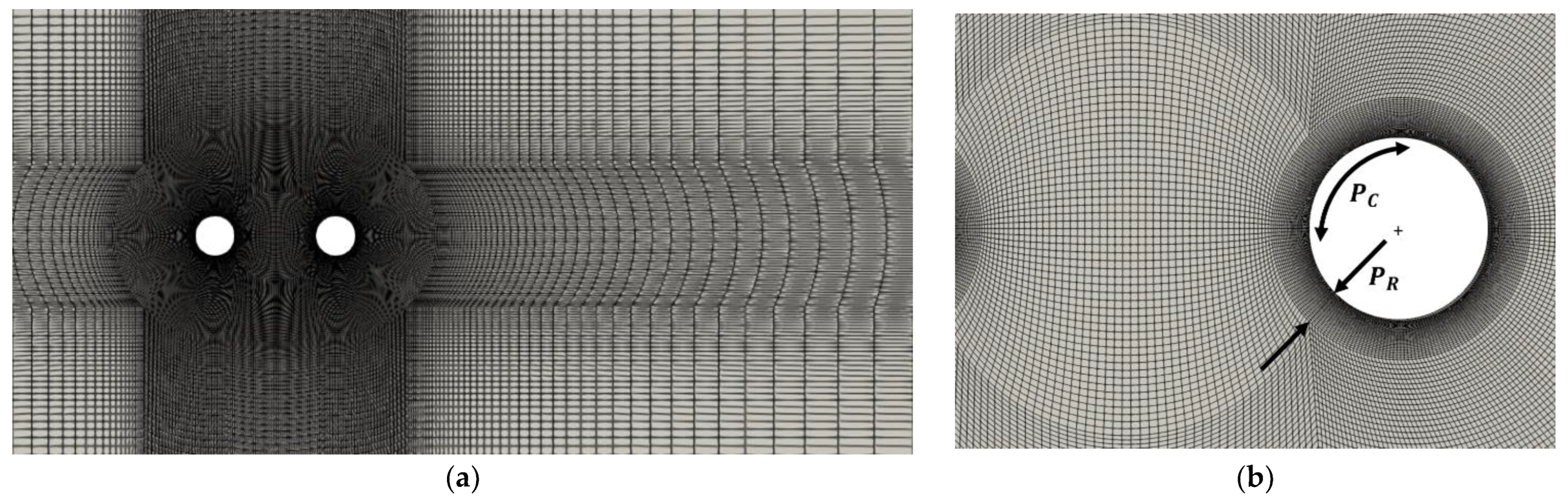
2.3. Computational Domain

The computational domain is shown in Figure 1. The center of the front cylinder is located at a distance $10 \mathrm{D}$ from the inlet boundary and $25 \mathrm{D}$ from the outlet boundary. The center of the back cylinder is located with a horizontal center-to-center offset $L$ from the front cylinder. The upper and lower boundaries are placed at the distance of $10 \mathrm{D}$ to the centers of both cylinders.

The boundary conditions used for the numerical simulations were set as follows:

1.

A uniform flow was specified at the inlet as:

$$u_1=U_{\infty },$$

(11)

$$u_{2 }=0,$$

(12)

$$k=\frac{3}{2}{\left(uI\right)}^2,$$

(13)

$$\omega =\frac{k^{0,5}}{{(C_{\mu })}^{0,25}l},$$

(14)

where $C_{\mu }=0.09$ is the model constant; $l=0.045 \mathrm{D}$ is the turbulent length scale; $I=1\%$ is the turbulent intensity.

2.

At the outlet of the domain, the velocities, $k$ and $\omega$ were set as zero normal gradient condition and the pressure was set to be zero.

3.

At the top and bottom of the domain, the velocities, the pressure, $k$ and $\omega$ were set as zero normal gradient.

4.

A no-slip boundary condition was applied for the velocities on the cylinder surfaces with $u_1=u_2=0$. A standard wall function was used to resolve the near-wall boundary layer. Therefore, a criterion of $30<y^{+}<40$ with $y^{+}$ was used, defined as:

$$y^{+}=\frac{u_{*}{h}_p}{v},$$

(15)

where $u_{*}$ is the friction velocity defined as:

$$u_{*}=\sqrt{\frac{{\tau }_{\omega }}{\rho }},$$

(16)

and ${\tau }_{\omega }$ is the wall shear stress.

2.4. Mesh Convergence and Validation Studies

The aim of the mesh convergence study was to determine the appropriate grid resolutions for the simulations. The convergence studies were conducted on three computational grids, shown in

Table 1. Results of grid convergence study.

Case	No. of Cells	${\overline{\mathit{C}}}_{\mathit{D}}$	${\mathit{C}}_{\mathit{L},\mathit{r}\mathit{m}\mathit{s}}$	$\mathit{S}\mathit{t}$
M1	74,496	0.4657	0.1565	0.3227
M2	113,256	0.4706	0.1599	0.3293
M3	171,970	0.4639	0.1553	0.3221

, with a different number of cells for the single cylinder case. An example of the mesh for the case M1 in Table 1 is shown in Figure 2. The geometry of each grid was kept similar. The time step ($∆t$) used in the mesh convergence study was chosen such that a maximum Courant number (defined as $Co=u·∆t/∆x$ where $u$ is the velocity magnitude of the flow and $∆x$ is the computational cell size) at each time step was below 0.5. The difference in the cell number was approximately 50% between cases.

Table 1 presents the results of the grid convergence study of the single cylinder case. The results showed that the relative difference of the time-averaged drag coefficient (the drag coefficient $C_D$ is defined as $F_D/\left(0.5\rho D{U}_{\infty }^2\right)$, where the force acting on the cylinder in the streamwise direction per unit length and the time-averaged values was calculated as ${\overline{C}}_D=\frac{1}{n}{\displaystyle \sum }_{i=1}^n{C}_{D,i})$ between cases, was lower than 2%. The relative difference of the root-mean-square values of the lift coefficient (the drag coefficient $C_L$ is defined as $F_L/\left(0.5\rho D{U}_{\infty }^2\right),$ where the force acting on the cylinder in the cross-stream direction per unit length and the root-mean-square value was defined as $C_{L,rms}=\sqrt{{\displaystyle \sum }_{i=1}^n{\left(C_{L,i}-{\overline{C}}_L\right)}^2/n}$), was lower than 5%, and the relative difference of the Strouhal number (defined as $St=f_{v}D/U_{\infty }$, where $f_v$ is the vortex shedding frequency obtained by performing fast Fourier transform of the time histories of the lift force coefficient $C_L$ of the cylinder) was lower than 3% between cases. According to the Table 1, the results suggested that for the computational grids with a cell number higher than approximately 113,000, a further grid refinement showed a slight influence on the obtained hydrodynamic quantities. Therefore, it could be concluded that the mesh of the case M2 could provide sufficient grid resolution for the simulations.

The obtained hydrodynamic coefficients are compared with the previously published experimental and numerical simulation data in

Table 2. Numerical and experimental data of a fixed single cylinder at high Reynolds number regime.

Source/Author	Method	$\mathit{R}\mathit{e}$	${\overline{\mathit{C}}}_{\mathit{D}}$	${\mathit{C}}_{\mathit{L},\mathit{r}\mathit{m}\mathit{s}}$	St
Present study	2D URANS $k-\omega SST$	$3.6\times {10}^6$	0.4706	0.1599	0.3293
Ong et al. (2009) [2]	2D URANS $k-\epsilon$	$3.6\times {10}^6$	0.4573	0.0766	0.3052
Porteous et al. (2015) [33]	2D URANS $k-\omega SST$	$3.6\times {10}^6$	0.4206	-	0.1480
Pang et al. (2016) [34]	2D URANS $k-\omega SST$	$5.2\times {10}^6$	0.4570	0.1847	0.3210
Janocha et al. (2021) [35]	2D URANS $k-\omega SST$	$3.6\times {10}^6$	0.4616	0.1750	0.3204
Jones et al. (1969) [36]	Experiments	$\left(0.5-8\right)\times {10}^6$	0.15–0.54	-	-
Shih et al. (1993) [37]	Experiments	$\left(1-5\right)\times {10}^6$	0.16–0.50	-	-
Schmidt (1996) [38]	Experiments	$\left(0.3-8\right)\times {10}^6$	0.18–0.53	-	-

. Generally, the ${\overline{C}}_D$ predicted in the present simulation was within the range of the experimental data and in reasonable agreement with the numerical simulation results. However, the $C_{L,rms}$, which was more sensitive than the value of ${\overline{C}}_D$, was different from the obtained value of $C_{L,rms}$ reported by Ong et al. (2009) [2], where the $k-\epsilon$ turbulence model was applied. However, the present predicted values were close to those reported by Porteous et al. (2015) [33] and Pang et al. (2016). The value of $St$ was higher than the value predicted by Porteous et al. (2015) [33] but close to the data reported by Ong et al. (2009), Pang et al. (2016) [34] and Janocha et al. (2021) [35]. To sum up, a general agreement with the published data could be achieved by the present numerical model. Therefore, the numerical model could be used for further investigation of the instantaneous flow structures and hydrodynamic properties around tandem cylinders. An example of the mesh used in the study for two tandem cylinders for $L/D=3$ is shown in Figure 3. The mesh of the near cylinder wall region was refined to accurately predict the flow features in that area. Mesh distribution around the cylinders could be described by $P_C$ and $P_R$ parameters, which are presented in Figure 3b. The value $P_C=220$ is the total number of points in circumferential direction along the cylinder surface and $P_R=41$ is the number of nodes in radial orientation.

3. Results

The effect of the center-to-center offset between two cylinders on the instantaneous flow structures, hydrodynamic quantities and $St$ were analyzed for $L/D=1.56, 1.8, 2.5, 3, 3.7, 4.$ Furthermore, DMD was applied to the velocities and pressure data in the 2D XY-plane flow field to extract the spatiotemporal information of the coherent flow structures in the wake regions of the UC and DC.

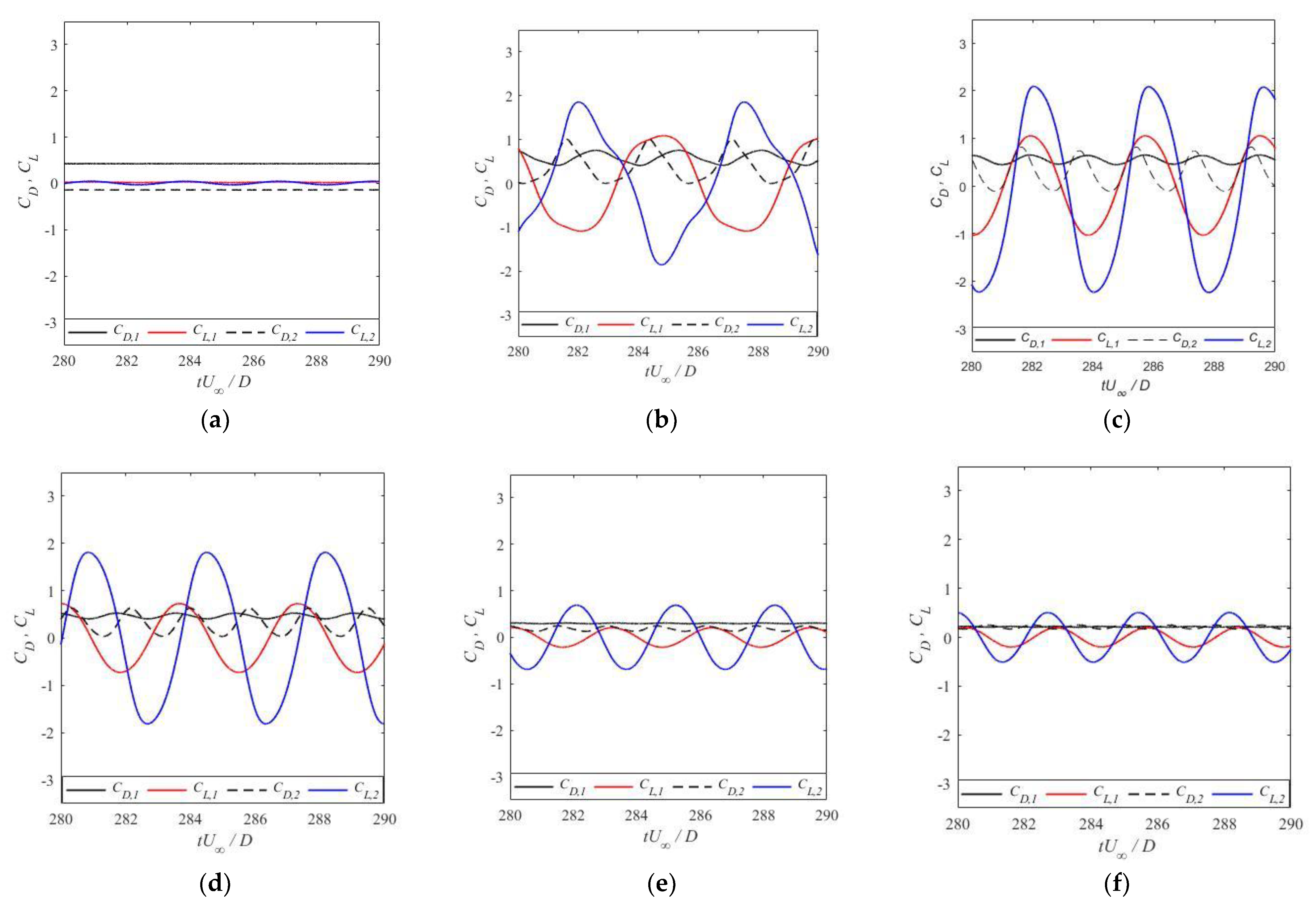
3.1. Hydrodynamic Forces

The hydrodynamics forces are analysed in this section in terms of the instantaneous drag and lift coefficients of the two tandem cylinders.

Figure 4 presents the time histories of $C_L$ and $C_D$ for $L/D=1.56, 1.8, 2.5, 3, 3.7 \mathrm{and} 4$. As seen from Figure 4, the $C_D$ oscillated at a frequency which was twice the $C_L$ of the cylinders. The pressure distribution around the cylinder underwent a periodic change as the vortex shedding grew, resulting in periodic variation in the force. The drag force was always positive due to the stagnation point at the front surface of the cylinders, in comparison with the lift force which could be positive and negative. Two vortices of almost equal strength and opposite signs were shed each oscillation period in the wake of a cylinder. Each vortex contributed to the maximum positive value of $C_D$ and contributed to the maximum values with opposite signs of $C_L$. Therefore, two positive peaks of the $C_D$ and two negative and positive peaks per one cycle of vortex shedding were seen. It resulted in a period doubling of the $C_D$ compared to the oscillation of the $C_L$.

According to Figure 4, the value of $C_D$ of the UC increased when the distance between UC and DC reduced. In contrast, the value of $C_D$ for the DC underwent a nonmonotonic change with shortening of the space between the two cylinders due to shielding effect. At $L/D=1.56$, $C_D$ of the DC was negative, as presented in Figure 4a. This was related to the cavity flow in the gap between UC and DC. In addition, $C_D$ fluctuation amplitude of the DC was higher in comparison with the UC for distance ratios $L/D=1.8, 2.5, 3, 3.7$ and $4,$ as shown in Figure 4. The UC shear layers reattached to the DC surface and contributed to the pressure distribution around the DC. However, at $L/D=1.56$, the values of $C_D$ of the UC and DC were approximately constant, as shown in Figure 4a. A possible reason was that the shear layers of the UC overshot the DC. Therefore, the two cylinders behaved as an extended body at $L/D=1.56$.

According to Figure 4b–d, the fluctuation amplitudes of $C_L$ were large in comparison with other cases. This might have been connected with the reattachment flow regime which triggered strong interaction of shear layers between UC and DC. A small angle of the UC shear layers reattachment to the front part of the DC caused strong vortex shedding behind the DC, and vice versa, which influenced the values of $C_L$. In addition, at $L/D=1.8$, the shape of the oscillating time history of $C_L$ was not sinusoidal, which indicated a strong modulation of the $C_L$ for both cylinders, as shown in Figure 4b. For $L/D=3.7$ and 4, the fluctuation amplitudes of $C_L$ were smaller in contrast to $L/D=1.8, 2.5$ and $3$. The reason might have been connected with a change of the flow pattern around the tandem cylinders caused by the increasing distance between the two cylinders.

Table 3. The values of $C_{L,rms}$ and $\overline{C_D}$ for different distance ratios.

$\mathit{L}/\mathit{D}$	${\mathit{C}}_{\mathit{L},\mathit{r}\mathit{m}\mathit{s}}$		$\overline{{\mathit{C}}_{\mathit{D}} }$
	UC	DC	UC	DC
1.56	0.0271	0.0283	0.4279	−0.1376
1.8	0.8352	1.1848	0.5845	0.3969
2.5	0.7512	1.5898	0.5456	0.2740
3	0.5234	1.3160	0.4707	0.3106
3.7	0.1447	0.4911	0.3031	0.1875
4	0.1394	0.3580	0.2169	0.2120

represents the values of $C_{L,rms}$ and $\overline{C_D}$ for different distance ratios. According to Table 3, the value of the $\overline{C_D}$ of the DC was smaller in comparison with UC for all distance ratios. The DC was located in the wake region of the UC. Therefore, the shielding effect caused by the UC influenced the flow pattern around the DC. However, the values of $\overline{C_D}$ of the DC achieved maximum values at $L/D=1.8$ and $3,$ as presented in Table 3. This might have again been connected with the transitions of the instantaneous flow structures between $L/D=1.8$ and $L/D=2.5$, and $L/D=2.5$ and $L/D=3$.

As shown in Table 3, the values of the $C_{L,rms}$ for both UC and DC became large when the distance between two cylinders reduced. At $L/D=2.5$, the value of the $C_{L,rms}$ of the DC achieved a maximum value. This might have been related to the dominance of the front reattachment (FR) flow regime, which caused strong vortex shedding behind the DC. However, the value of the $C_{L,rms}$ of both cylinders decreased drastically at $L/D=1.56$. The possible reason was that the overshoot flow regime dominated at $L/D=1.56$ and the interaction of UC and DC shear layers was minimized.

Figure 5 shows the mean pressure coefficient around the UC and DC for $L/D=1.56$. According to Figure 5, the front surface of the DC had a low negative pressure, which was almost the same as the corresponding value of the base pressure of the UC. This fact was an indication that the flow in the gap between UC and DC was almost stagnant. Furthermore, the negative pressure coefficient on the front side of the DC exceeded that on its back surface. Therefore, the DC experienced a negative drag force.

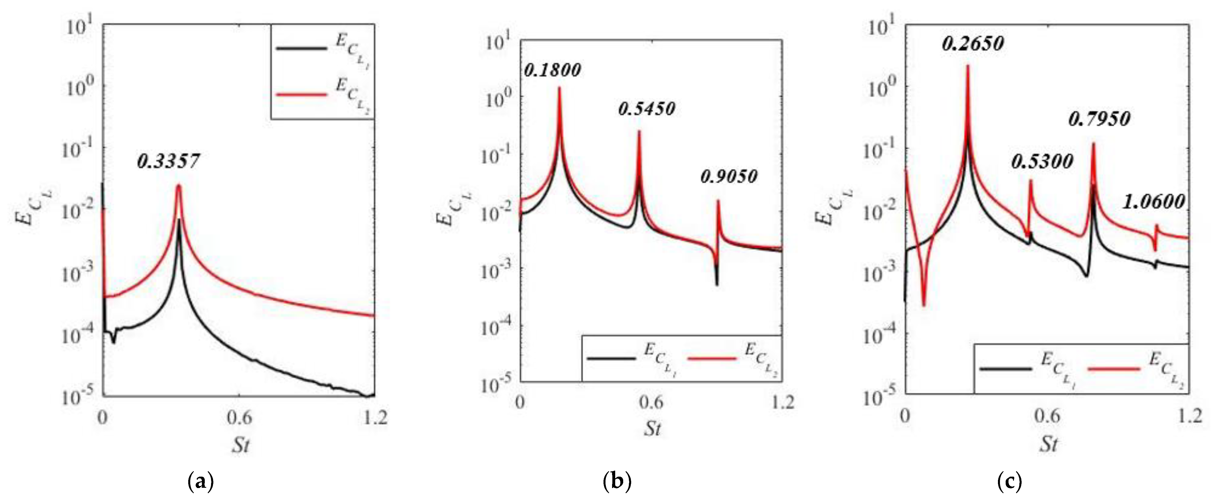
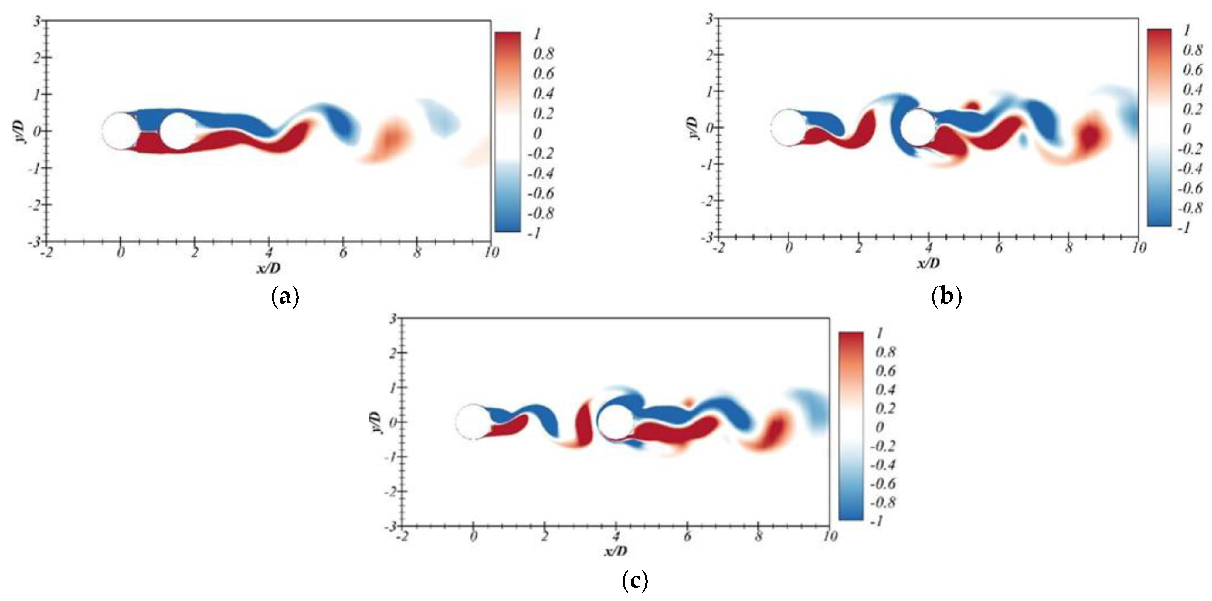
3.2. Strouhal Number and Flow Structures

The relationship between $St$ and flow structures around tandem cylinders is analysed in this section. Figure 6 presents the PSD (Power Spectral Density) functions $E_{C_{L_1}}$ and $E_{C_{L_2}}$ of $C_L$ for $L/D=1.56, 1.8, 2.5, 3, 3.7 \mathrm{and} 4$ of the UCs and DCs, respectively. For all considered cases, the values of $St$, and its harmonics of the DC, dominated at the same frequency as measured for the UC. This was explained by Meyer et al. (2011) [39] as follows: when $L/D$ is less than 8 the vortices of the UC can trigger the vortex shedding from the DC, leading to a lock-in of UC and DC vortex shedding.

According to Figure 6a,b, the value of $St$ decreased from 0.336 to 0.180 when $L/D$ increased from 1.56 to 1.8. The decrease was connected to change in the flow structure. Instantaneous contours of the spanwise vorticity for $L/D=1.56$ are presented in Figure 7a. At $L/D=1.56,$ where over-shoot flow regime dominated, as shown in Figure 7a, the value of $St$ was close to that of an isolated cylinder ($\approx 0.329,$ as presented in Table 2). When the over-shoot regime dominated, the DC was located inside the recirculation region behind the UC. The separated shear layers of the UC overshot the DC without reattachment before rolling up into a Karman vortex street, as shown in Figure 7a. Therefore, only one $St$ was observed, shown in Figure 6a.

The spanwise vorticities for $L/D=1.8$ at different time steps are shown in Figure 8. Meyer et al. (2011) [39] suggested a division of the cylinder surface to the following zones: front ($\theta =0^{°}~{60}^{°}$), front-side ($\theta ={60}^{°}~{90}^{°}$), rear-side $(\theta ={90}^{°}~{120}^{°})$ and rear ($\theta ={120}^{°}~{180}^{°}$) ($\theta$ is presented in Figure 9). According to the surface division, front-side reattachment regime dominated at $L/D=1.8,$ as shown in Figure 8a. Three peaks, including the third and fifth harmonics of $St,$ were observed in the PSD, as shown in Figure 6b at $L/D=1.8$. The first $St$ was connected to the vortex shedding. The multiple peaks in the PSD were due to the reattachment of the shear layer on the DC. The lower shear layer of the UC reattached on the upper part of the DC at the front-side surface, as seen in Figure 8a. Then, the reattached shear layer split into two vortex slices going through the lower and upper part of the DC. The upper reattached vortex slice went to the upper side of the DC and further separated from its surface. It did not seem to influence the negative vortex behind the DC, as shown in Figure 8b. At the same time, a positive vortex began to grow and was about to move up, as denoted by the arrow in Figure 8b. Then, this positive vortex would go down to merge the split reattached vortex slice from the UC, as shown in Figure 8c. This flow pattern also happened with the opposite vortex signs, as shown in Figure 8d, and this might have been associated with the third harmonic of $St,$ in Figure 6b.

Four peaks, including the second, third and fourth harmonics of $St,$ were observed in the PSD, as shown in Figure 6c at $L/D=2.5$. As shown in Section 3.1, $C_{L,rms}$ of the DC achieved a higher value at $L/D=2.5,$ compared with $L/D=1.8$ and $3$. It meant that the shear layers reattached on the surface of the DC at a smaller $\theta$ at $L/D=2.5$ in comparison with that for $L/D=1.8$ and $3$. Therefore, the flow pattern changed from front-side reattachment (FSR) to FR at $L/D=2.5$. The spanwise vorticities for $L/D=2.5$ at different time steps are shown in Figure 10. According to Figure 10a, the shear layer of the UC reattached on the front surface of the DC at $L/D=2.5$ and divided into the upper and lower vortex slices. The upper vortex slice would interact with the negative vortex shedding from the DC, as shown in Figure 10b. At the exact same time, a positive vortex began to grow behind the DC and also moved up to interact with the negative vortex, as denoted by the arrow in Figure 10b. This interaction between three vortices might have been associated with the second harmonics of $St,$ as shown in Figure 6c. Then, after the negative vortex separated, the positive vortex behind the DC went down and merged with the reattached lower positive vortex slice from the UC, as shown in Figure 10c. The flow pattern was the same as that shown for $L/D=1.8$ and occurred with the opposite vortex signs, as shown in Figure 7d. Again, this flow pattern was related to the third harmonics of $St$.

At $L/D=3$, two peaks, including the third harmonic of $St,$ were observed in the PSD, as shown in Figure 6e. At $L/D=3$, the flow pattern changed from FR to the FSR. This was indicated by the decreasing $C_{L,rms}$ at $L/D=3$ in comparison with $L/D=2.5$. The reason was that at $L/D=3$, the shear layers reattached to the surface of the DC at a bigger $\theta$ compared to those at $L/D=2.5$ and produced weaker Karman vortices behind it. A detailed development of vorticity structures for $L/D=3$ at different time steps is shown in Figure 11.

The lower shear layer of the UC reattached on the front-side surface of the DC, as presented in Figure 11a. After that, the reattached shear layer split into two into two vortex slices moving through the lower and upper parts of the DC, as shown in Figure 11b. The upper vortex slice went upper side of the DC and then separated from its surface. It seemed that the upper vortex slice did not contribute to the development of the negative vortex behind the DC, as shown in Figure 11b. Simultaneously, the positive vortex was growing and moving up, as depicted by the arrow in Figure 11b. Furthermore, the positive vortex would move down and merge with the lower vortex slice from the reattached shear layer of the UC, as presented in Figure 11c, and this might have been associated with the third harmonic of $St$ in Figure 6d. This flow pattern also repeated with the opposite vortex signs, as shown in Figure 11d. Therefore, the evolution of the flow pattern around tandem cylinders at $L/D=3$ was similar to the development of the vortical structures around UC and DC at $L/D=1.8$.

$St$ was again about 0.329 for $L/D=3.7$, indicating that the flow pattern changed. Alam et al. (2011) proposed that at $Re=9.7\times {10}^3$ and $Re=6.5\times {10}^4$ a bi-stable regime exists between the FR and co-shedding flows at the distances of $3.5<L/D<3.9$ and $3.9<L/D<4.2$, respectively. Therefore, it could be concluded that $L/D=3.7$ and 4, shown in see Figure 7b,c belonged to the bi-stable flow regime as the present investigation was performed for $Re=3.6\times {10}^6$. In line with Figure 6e,f, two peaks were observed in the PSD. The second peak, which was characterized by a small amplitude, was the third super-harmonic of the first one. The influence of the third super-harmonic was negligible for $L/D=3.7$ and $4$.

Figure 12 presents the time-averaged flow streamlines and pressure field. The cavity flow indicated by the strong recirculation motions appeared in the gap between the two cylinders, as shown in Figure 12a. The low pressure at the surface of the DC caused a dramatic change in its ${\overline{C}}_D$, which has been explained in Section 3.1. According to Figure 12b,c, the two recirculation motions behind the DC disappeared, resulting in an attached flow around the DC for $L/D=1.8$ and $2.5$. The probable reason was that the high transverse interactions of the shear layers resulted in a delayed separation point, which suppressed the two recirculation motions. However, the recirculation bubbles reappeared for $L/D\ge 3$, as shown in Figure 12d–f. A possible reason was that the influence of the UC shear layers was not sufficient to influence the separation point in the boundary layer of the DC. The behaviour of the DC boundary layer became close to that of a single cylinder.

As a summary, the values of $St$ for different distance ratios are presented in

Table 4. Summary of the $St$ values and different flow regimes.

$\mathit{L}/\mathit{D}$	$\mathit{S}\mathit{t}$		Flow Regime
	UC	DC
1.56	0.3357	0.3357	Overshoot
1.8	0.1800	0.1800	FSR
2.5	0.2650	0.2650	FR
3	0.2750	0.2750	FSR
3.7	0.3200	0.3200	Bi-stable
4	0.3650	0.3650	Bi-stable

. At $L/D=1.56$ and $3.7$ the value of $St$ was close to that of an isolated cylinder ($\approx 0.329$). It was related to the change of the flow regime, as discussed previously and presented in Table 4. At $L/D=1.8$, this distance ratio created a longer length of the combined tandem structure which caused a reduction of the $St$ value, compared with that at $L/D=1.56$. According to Table 4, the value of $St$ gradually became close to the value of a single cylinder case with further enlargement of the distance between the two cylinders.

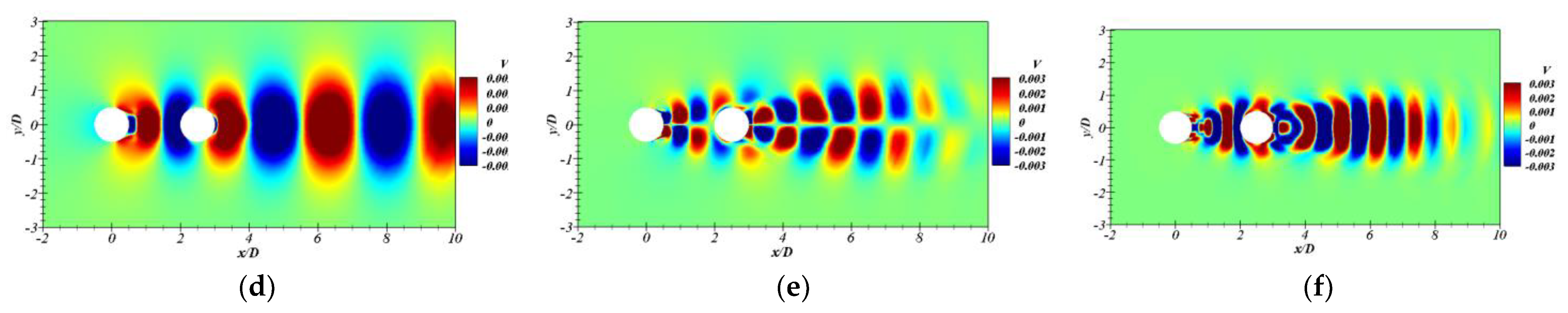
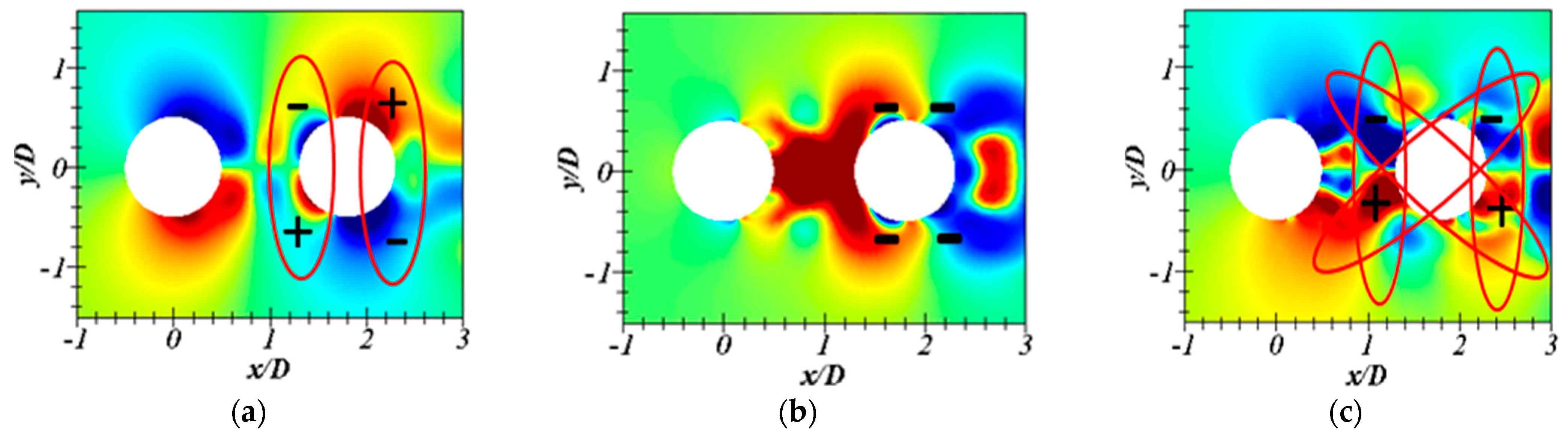
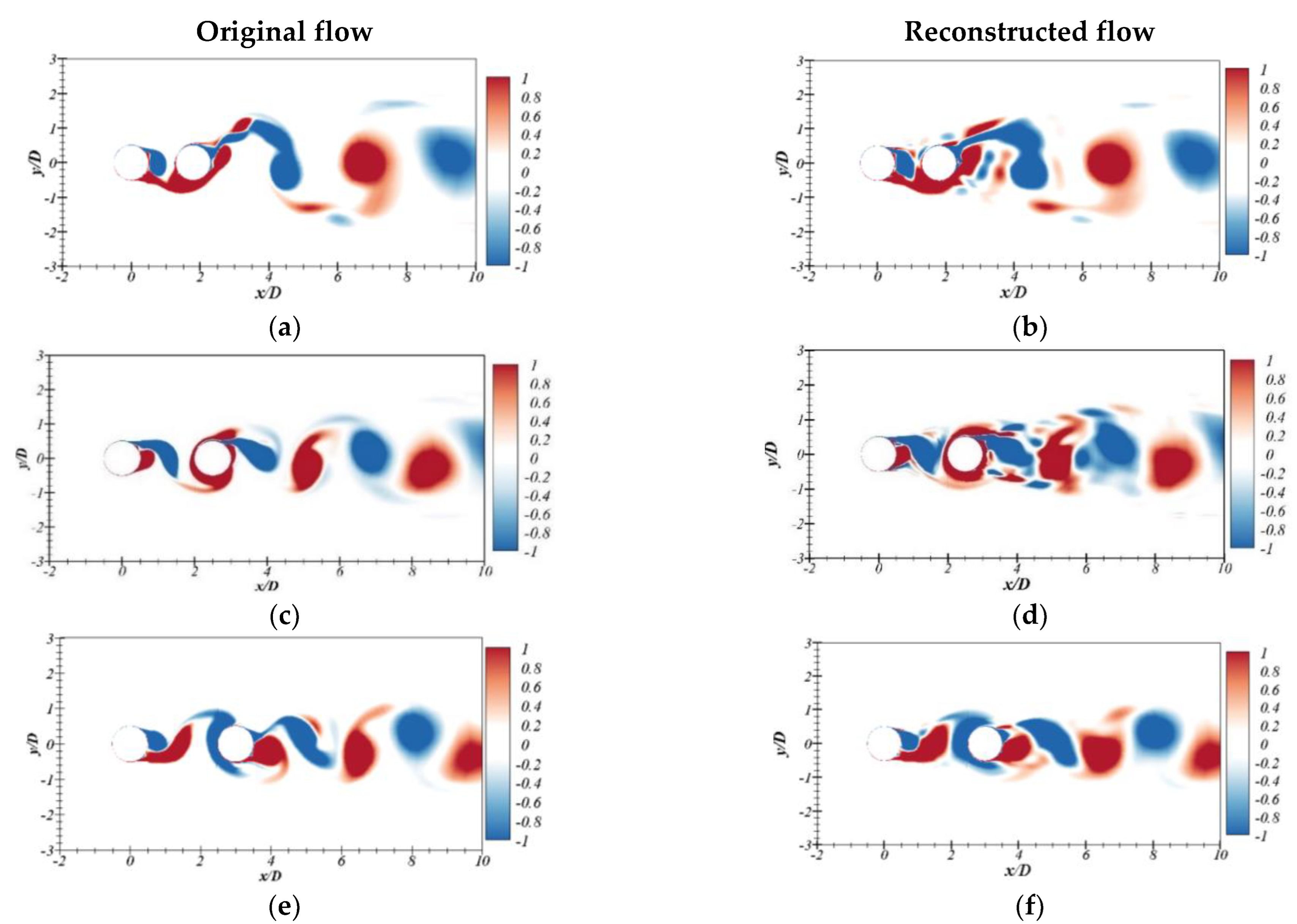
3.3. Dynamic Mode Decomposition Analysis

The DMD method proposed by Schmid (2010) [40] was implemented in the present study to get a good understanding of the spatial distribution of the coherent structures related to the dominant frequencies, shown in Section 3.2. The method allows approximation of the flow fields obtained by numerical simulations or experiments using a linear combination of the DMD modes and further develops a reduced order representation of the dynamical system as:

$${\Psi }_0=\left[u_1, u_2, u_3, . . . ,u_N\right]\approx \Phi D_{\alpha }{V}_{\mathrm{and}}=\left[{\mathsf{\phi }}_1, {\mathsf{\phi }}_2, {\mathsf{\phi }}_3, . . . ,{\mathsf{\phi }}_N\right]\left[\begin{array}{ccc}{\alpha }_1& \dots & \dots \\ \dots & \cdots & \dots \\ \dots & \dots & {\alpha }_N\end{array}\right]\left[\begin{array}{ccc}{\mu }_1^0& \cdots & {\mu }_1^{N-1}\\ ⋮& \ddots & ⋮\\ {\mu }_N^0& \cdots & {\mu }_N^{N-1}\end{array}\right],$$

(17)

where ${\Psi }_0$ is a matrix consisting of flow fields $u_i$ ($i=1,2,\dots N$) at each time step and $u_i$ stores flow data, such as the flow velocities and pressure at each spatial point; $\Phi$ represents the matrix consisting of the spatial DMD modes ${\mathsf{\phi }}_i$, $D_{\alpha }=\mathrm{diag}\left({\alpha }_1, . . . ,{\alpha }_N\right)$ represents the amplitudes of the corresponding modes within the time span and $V_{\mathrm{and}}$ denotes the Vandermonde matrix, which contains the temporal variations of each mode during the investigated time span. Schmid (2010) [26] states that $\mathrm{Im}\left(\log \left({\mu }_i\right)/\mathsf{\Delta }t\right)$ represents the frequency and $\mathrm{Re}\left(\log ({\mu }_i\right)/\mathsf{\Delta }t)$ demonstrates the amplification rate of the mode.

A key problem in the DMD method is the selection of a small subset of DMD modes which can provide a reduced order approximation of the original dynamical system. However, the contribution of each DMD mode to the dynamic system is difficult to quantify, due to the lack of information of its energy obtained through the original DMD algorithm. Therefore, Jovanovic et al. (2014) [40] proposed a sparsity-promoting DMD (SPDMD) method to select a finite number of dynamically important modes within the time span. To achieve this, a positive regularization parameter $\gamma$ is used to maintain a balance between the approximation error and the number of selected dominant DMD modes. An optimization problem is solved to obtain the unknown elements of the matrix $D_{\alpha }$:

$$\underset{\alpha }{\min }\Vert {\Psi }_0-\Phi D_{\mathsf{\alpha }}{V}_{and}\Vert {}_F^2+\gamma {\displaystyle \sum }_{i=1}^N\left|{\alpha }_i\right|,$$

(18)

where ${\Vert \dots \Vert }_F$ is the Frobenius norm of a matrix. Usually, a large value of $\gamma$ will introduce a high limitation on the number of non-zero elements in $D_{\alpha }=\mathrm{diag}\left({\alpha }_1, \dots ,{\alpha }_N\right)$. Therefore, the SPDMD algorithm removes the modes which are only of influence for a short time in the early stages of the time evolution and are damped rapidly and also the modes with small amplitudes, as reported in Jovanovic et al. (2014) [40]. As a result, the DMD modes which contribute the most to the dynamic system are retained. Various applications of this method can be found in Yin & Ong (2020, 2021) [41,42] and Janocha et al. (2021) [35].

The present analysis was performed on the velocity and pressure data obtained in the computational domain. The number of the snapshots was $N=260$ with a time step of $∆tD/U_{\infty }=0.5$ for $L/D=1.8, 2.5$ and $3$. The distance ratios were chosen to show how the second and third harmonics of $St$ influenced the mode pattern.

Figure 13 shows the DMD eigenvalues for $L/D=1.8, 2.5$ and $3$. The modes which were located inside the unit circle were damped within the temporal evolution of the dynamical system because of their negative growth rate. Most of the eigenvalues lay on the unit circle, indicating that they were ‘neutrally stable’ with almost zero growth/decay rate. This was because of the statistically stationary state of the wake flow, as reported in Schmid (2010) [26], Jovanovic et al. (2014) [40] and Pan et al. (2015) [43].

Figure 14 shows the DMD spectra obtained using the DMD algorithm and the modes selected by using the SPDMD algorithm. The total number of the selected modes corresponded to $N_{sp}=7, 9$ and $7$ for $L/D=1.8, 2.5$ and $3$, respectively. According to Figure 14, among the chosen modes, by using the SPDMD algorithm, the most dominant mode corresponded to the time-averaged flow with a zero frequency. The rest of the modes determined the large-scale fluctuating flows, which appeared in pairs with positive and negative oscillation frequencies.

Table 5. Energy levels of the DMD modes and their respective contributions to the total energy.

$\mathit{L}/\mathit{D}$	Mode 1	Mode 2	Mode 3
	Cumulative Energy, %
1.8	85.70	92.85	95.35
2.5	87.10	93.55	94.02
3	93.60	96.33	98.17

provides the ratios of the energy contribution of the DMD modes selected by using the SPDMD algorithm to the total energy of the system for $L/D=1.8, 2.5$ and 3. According to Table 5, the SPDMD algorithm allowed the capturing of a few of the most dominant modes which contained more than 94% of the system energy and almost reflected the entire spatial distribution of the flow structure in the flow field.

A comparison between the PSD of the $C_L$ of the DC and the DMD spectrum was performed, as indicated in Figure 15. Modes chosen by using the SPDMD algorithm could correspond well to the different frequency peaks in the PSD. According to Figure 15b, more modes were required to completely reproduce the dynamic information of the coherent flow structures in the wake regions behind both UC and DC for distance ratio $L/D=2.5,$ due to the flow complexity compared with the other two cases. As has been explained in Section 3.2, there are strong interactions between the shear layers with large amplitudes of transverse oscillation behind the UC and DC. Therefore, several peaks were observed in PSD at $L/D=2.5$.

The modes are supposed to display spatial distribution and length scale features of the flow structures. Figure 16, Figure 17 and Figure 18 show the spatial structures of velocity modes selected by the SPDMD method for $L/D=1.8, 2.5$ and $3$. The streamwise velocities of Modes 1 and 3 revealed a top–bottom mirrored symmetry with respect to the centreline of the cylinders, while the cross-flow velocities displayed asymmetry. The two velocity components of Mode 2 showed reverse symmetry properties compared with Modes 1 and 3. In addition, with the increasing frequency and decreasing amplitude of the higher order modes, the length scale of the structures became smaller. Especially for Mode 3, the energetic streamwise velocity structures were located near the shear layers in the wake regions behind the UC and DC indicating the oscillating features of the shear layers.

Figure 19 shows the spatial structures of pressure modes selected by the SPDMD method for $L/D=1.8, 2.5$ and $3$. For the pressure distribution of the modes, there were positive and negative regions around the two cylinders, indicating a periodic changing of forces acting on the cylinders. In the cross-flow direction, if the positive and negative regions formed a pair, as indicated by the red circle in Figure 19, it would contribute to the lift force at the corresponding frequency of the mode. However, Mode 2 for $L/D=1.8$ and 3.0 had similar distribution of the pressure, especially around the DC, as shown in Figure 19b,h. It had negative pressure regions around both the two sides, which had no contribution to the lift force. Therefore, although Mode 2 was identified by SPDMD, there was no peak in the frequency spectra at the second harmonic of St. For $L/D=2.5$, on the contrary, there were both positive and negative pressure regions around the DC, which contributed to the lift force at the second harmonic of St.

By using the extracted dominant DMD modes, a reduced-order representation of the flow field could be reconstructed. The snapshots of the vorticity at $∆tD/U_{\infty }=280$ for the original numerical simulations and reconstructed flow fields are presented in Figure 20 for $L/D=1.8, 2.5$ and $3$. The DMD mode shapes, with their corresponding amplitudes and frequencies, obtained by the SPDMD algorithm were used to create the reduced-order representations. The velocity and pressure at a point ($x,y$) and $t=t_n$ were reconstructed by:

$$u\left(x,y,t_n\right)={\displaystyle \sum }_{i=1}^{N_{sp}}{\alpha }_i{\phi }_i\left(x,y\right){\mu }_i^{n-1},$$

(19)

$$p\left(x,y,t_n\right)={\displaystyle \sum }_{i=1}^{N_{sp}}{\alpha }_i{\phi }_i\left(x,y\right){\mu }_i^{n-1},$$

(20)

where $N_{sp}$ is the total number of SPDMD modes. As shown in Figure 20, in comparison with the original flow fields, it was evident that the SPDMD method could successfully reconstruct the main flow features, although the investigated flow was complicated at a high Reynolds number. The reconstructed flow field had some differences in the wake region of the DC for $L/D=2.5,$ where there were strong interactions of shear layers in the flow, as shown in Figure 20d. The noisy structures in the reconstructed wake flow behind the DC could be removed by including more DMD modes.

Figure 21 and Figure 22 show the time histories of the lift and drag coefficients of the UC and DC obtained by the numerical simulations and the reduced-order representations. It can be seen that the reduced-order representations with a considerably small number of modes could correctly reproduce the time histories of the lift and drag coefficients. Thus, the frequencies and amplitudes of the dominant DMD modes, which contributed the most to the dynamics, were obtained accurately by the SPDMD algorithm.

4. Conclusions

The flow around two tandem cylinders with different horizontal offsets of $L/D=1.56, 1.8, 2.5, 3, 3.7$ and $4$ was investigated numerically at a Reynolds number of $3.6\times {10}^6$. The 2D URANS equations with a standard $k-\omega \mathrm{SST}$ turbulence model were solved. Verification and validation studies were performed for the flow past a single cylinder and showed that the present numerical model could provide satisfying results compared with the previously published data. Then, the numerical model was used to study the hydrodynamic characteristics of tandem cylinders subjected to high $Re$ incoming flow. Analysis of instantaneous flow structures, hydrodynamic coefficients, $St$ and vortical structures were demonstrated in the present study. In addition, the SPDMD algorithm was implemented to extract dominant modes which contributed the most to the inherent dynamics, and to construct a reduced-order representation of the flow field. The main conclusions can be summarized as follows:

1.

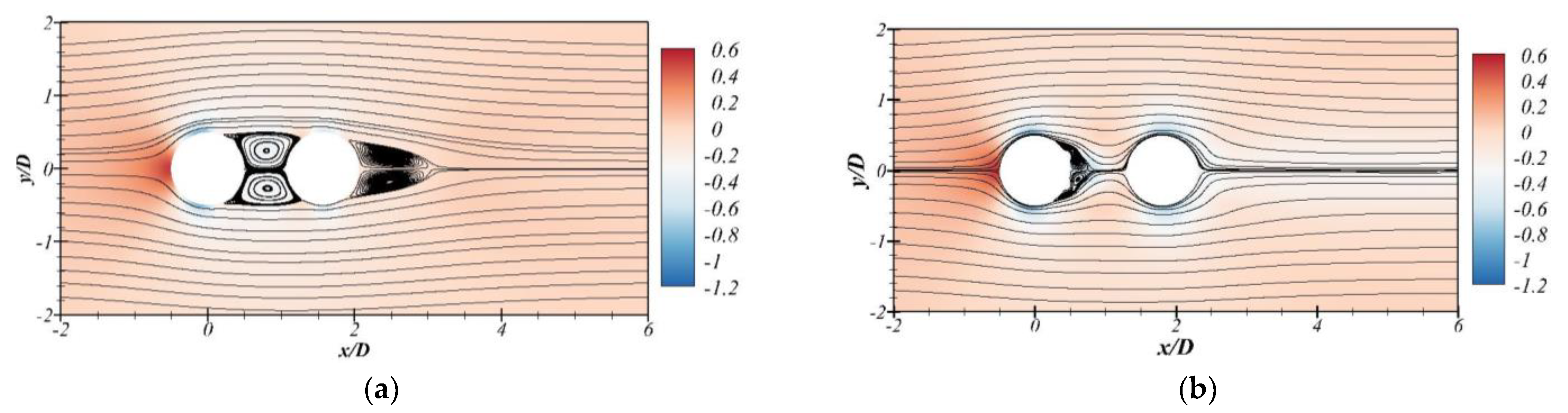
With the increasing $L/D$, flow structures at $Re=3.6\times {10}^6$ changed in terms of overshoot, FSR, FR, FSR and bi-stable. This relates to the reattachment point of the separated UC shear layers to the surface of the DC.

2.

The lower vorticity slice of the reattached shear layer to the surface of the DC contributed to the evolution of the positive vorticity behind the DC. It explains the existence of the third super-harmonic for the cases considered. However, the second harmonic observed in the spectra of the lift forces was only for the case of $L/D=2.5$. This relates to assistance of the upper vorticity slice of the reattached shear layer to the development of the negative coherent structure behind the DC.

3.

The values $C_{L,rms}$, $\overline{C_D}$ and $St$ were influenced by $L/D$ such that $\overline{C_D}$ decreased with a decreasing $L/D$ between two cylinders and achieved a negative value for the DC at $L/D=1.56$. The negative $\overline{C_D}$ value corresponded to a low pressure at the front surface of the DC caused by the cavity flow between UC and DC at $L/D=1.56$. Increasing amplitudes of $C_L$ fluctuation were found at $\frac{L}{D}=2.5,$ and this relate to FR flow, which causes significant interaction of shear layers. At $L/D\ge 1.8$, the reattachment flow regime (FR) dominated. It creates a longer after-body length of the combined UC and DC body leading to a sudden reduction of the $St$ value.

4.

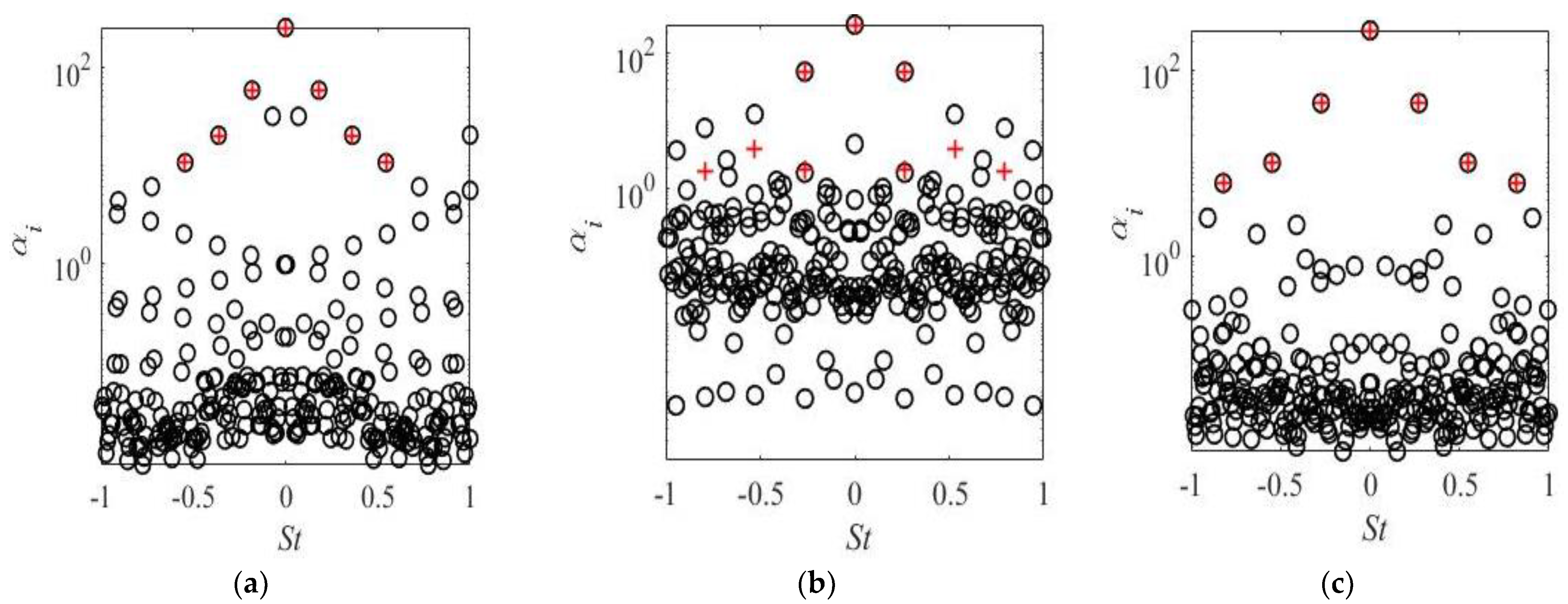
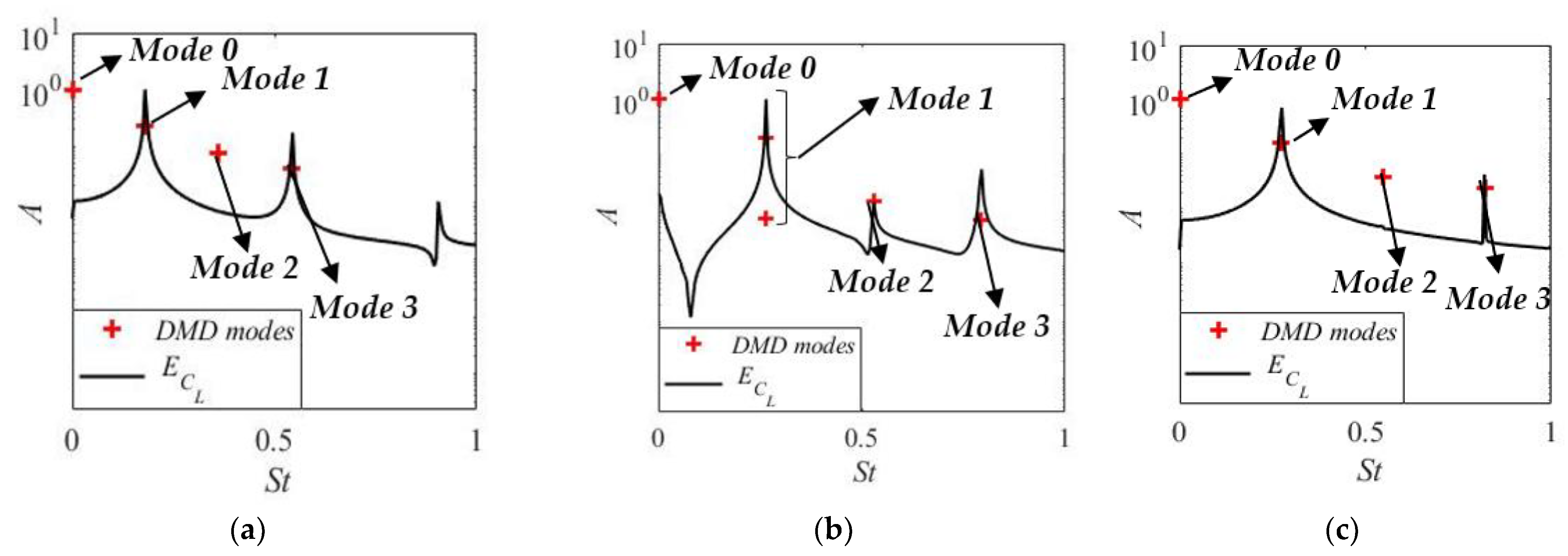
The SPDMD algorithm was used to extract a few dominant modes which contributed the most to the flow dynamics. It was found that Mode 2 for $L/D=1.8$ and $3$ did not contribute to the lift force. Therefore, there was no peak in the frequency spectra of the lift force at the second harmonic of $St$ for these two cases, although Mode 2 was identified by using SPDMD. In addition, the reduced-order representations of the flow field, which consist of the finite SPDMD modes number, can correctly reconstruct the wake flow at the investigated high Reynolds number.

References

- Sumer, B.; Fredsøe, J. Hydrodynamics around Cylindrical Structures; World Scientific Publishing Co., Pte. Ltd.: Singapore, 1997. [Google Scholar]
- Ong, M.C.; Utnes, T. Numerical simulation of flow around a smooth circular cylinder at very high Reynolds numbers. J. Mar. Struct. 2009, 22, 142–153. [Google Scholar] [CrossRef]
- Nakaguchi, H.; Hashimoto, K.; Muto, S. An experimental study on aero-dynamic drag of rectangular cylinders. J. Jpn. Soc. Aerospace Sci. 1968, 16, 1–5. [Google Scholar]
- Norberg, C. Flow around rectangular cylinders: Pressure forces and wake frequencies. J. Wind Eng. Ind. Aerodyn. 1993, 49, 187–196. [Google Scholar] [CrossRef]
- Ohya, Y. Note on a discontinuous change in wake pattern for a rectangular cylinder. J. Fluids Struct. 1994, 8, 325–330. [Google Scholar] [CrossRef]
- Okajima, A. Numerical simulation of flow around rectangular cylinders. J. Wind Eng. Ind. Aerodyn. 1990, 33, 171–180. [Google Scholar] [CrossRef]
- Tian, X.; Ong, M.C.; Yang, J.; Myrhaug, D. Unsteady RANS simulations of flow around rectangular cylinders with different aspect ratios. J. Ocean Eng. 2013, 58, 208–216. [Google Scholar] [CrossRef]
- Dutta, S.; Panigrahi, P.K.; Muralidhar, K. Experimental investigation of flow past a square cylinder at an angle of incidence. J. Eng. Mech. 2008, 134, 788–803. [Google Scholar] [CrossRef]
- El-Sherbiny, S. Flow separation and reattachment over the sides of a 90° triangular prism. J. Wind Eng. Ind. Aerodyn. 1983, 11, 393–403. [Google Scholar] [CrossRef]
- Nakagawa, T. Vortex shedding mechanism from a triangular prism in a subsonic flow. J. Fluid Dyn. Res. 1989, 5, 69–81. [Google Scholar] [CrossRef]
- Cheng, M.; Liu, G.R. Effects of afterbody shape on flow around prismatic cylinders. J. Wind Eng. Ind. Aerodyn. 2000, 84, 181–196. [Google Scholar] [CrossRef]
- Tritton, D. Experiments on the Flow past a circular cylinder al low Reynolds numbers. J. Fluid Mech. 1959, 6, 547–567. [Google Scholar] [CrossRef]
- Dimopoulos, H.; Hanratty, T. Velocity gradients at the wall for flow around a cylinder for Reynolds numbers between 60 and 360. J. Fluid Mech. 2006, 33, 303–319. [Google Scholar] [CrossRef]
- Park, J.; Kwon, K. Numerical solutions of flow past a circular cylinder at Reynolds numbers up to 160. KSME Int. J. 1998, 12, 1200–1205. [Google Scholar] [CrossRef]
- Rajani, B.; Kandasamy, A. Numerical simulation of laminar flow past a circular cylinder. J. Appl. Math. Medel. 2009, 33, 1225–1247. [Google Scholar] [CrossRef]
- Zdravkovich, M. Review of flow interference between two circular cylinders in various arrangements. J. Fluids 1977, 99, 618–663. [Google Scholar] [CrossRef]
- Sumner, D. Two circular cylinders in cross-flow: A review. J. Fluid Struct. 2010, 26, 849–899. [Google Scholar] [CrossRef]
- Zdravkovich, M. The effects of interference between circular cylinders in cross flow. J. Fluids 1978, 1, 239–261. [Google Scholar] [CrossRef]
- Hori, E. Experiments on flow around a pair of parallel circular cylinders. In Proceedings of the Ninth Japan National Congress for Applied Mechanics, Nagoya, Tokyo, 29 August–1 September 1959; Volume 11, pp. 231–234. [Google Scholar]
- Huhe-Aode; Tatsuno, M. Visual studies of wake structure behind two cylinders in tandem arrangement. Rep. Res. Inst. Appl. Mech. 1985, 32, 1–20. [Google Scholar]
- Nishimura, T.; Ohori, Y.; Kawamura, Y. Flow pattern and rate of mass transfer around two cylinders in tandem. J. Intern. Chem. Engin. 1986, 26, 123–129. [Google Scholar]
- Xu, G.; Zhou, Y. Strouhal numbers in the wake of two inline cylinders. J. Exp. Fluids 2004, 37, 248–256. [Google Scholar] [CrossRef]
- Alam, A. Two interacting cylinders in cross flow. J. Phys. Rev. E 2011, 84, 639–654. [Google Scholar] [CrossRef] [PubMed]
- Catalano, P.; Wang, M.; Iaccarino, G.; Moin, P. Numerical simulation of the flow around a circular cylinder at high Reynolds numbers. Int. J. Heat Fluid Flow 2003, 24, 463–469. [Google Scholar] [CrossRef]
- Hu, X.; Zhang, X.; You, Y. On the flow around two circular cylinders in tandem arrangement at high Reynolds number. J. Ocean Eng. 2019, 189, 106–301. [Google Scholar] [CrossRef]
- Schmid, P. Dynamic Mode Decomposition of numerical and experimental data. J. Fluid Mech. 2010, 656, 5–28. [Google Scholar] [CrossRef]
- Rowley, C.; Mezić, I.; Bagheri, S.; Schlatter, P.; Henningson, D.S. Spectral analysis of nonlinear flows. J. Fluid Mech. 2009, 22, 142–153. [Google Scholar] [CrossRef]
- Taira, K.; Brunton, S.L.; Dawson, S.T.; Rowley, C.W.; Colonius, T.; McKeon, B.J. Modal analysis of fluid flows: An overview. AIAA J. 2017, 55, 4013–4041. [Google Scholar] [CrossRef]
- Bagheri, S. Koopman-mode decomposition of the cylinder wake. J. Fluid Mech. 2013, 725, 596–623. [Google Scholar] [CrossRef]
- Hemati, M.S.; Rowley, C.W.; Deem, E.A.; Cattafesta, L.N. De-biasing the dynamic mode decomposition for applied Koopman spectral analysis of noisy datasets. Theor. Comput. Fluid Dyn. 2017, 31, 349–368. [Google Scholar] [CrossRef]
- Schmid, P.; Li, L.; Pust, O. Application of the dynamic mode decomposition. Theor. Comput. Fluid Dyn. 2011, 25, 249–259. [Google Scholar] [CrossRef]
- Menter, F.; Kuntz, M.; Langtry, R. Ten years of industrial experience with the SST turbulence model. J. Heat Mass Transf. 2003, 4, 625–632. [Google Scholar]
- Porteous, A.; Habbit, R.; Colmenares, J.; Poroseva, S.; Murman, S.M. Simulations of incompressible separated turbulent flows around two-dimensional bodies with URANS models in OpenFOAM. In Proceedings of the 22nd AIAA Computational Fluid Dynamics Conference 2015, Dallas, TX, USA, 22–26 June 2015. [Google Scholar]
- Pang, A.; Skote, M.; Lim, S.Y. Modelling high re flow around a 2D cylindrical bluff body using the k-ω (SST) turbulence model. J. Prog. Comput. Fluid Dyn. 2016, 16, 48–57. [Google Scholar] [CrossRef]
- Janocha, M. Numerical simulations of flow-induced vibrations of two rigidly coupled cylinders with uneven diameters in the upper transition Reynolds number regime. J. Mar. Struct. 2021, 105, 103–332. [Google Scholar]
- Jones, G.; Cincotta, J. Aerodynamic Forces on a Stationary and Oscillating Circular Cylinder at High Reunolds Numbers; Technical Report TB R-300; NASA: Washington, DC, USA, 1969.
- Shih, W.C.L.; Wang, C. Experiments on flow past rough circular cylinders at large Reynolds numbers. J. Wind Eng. Aerodyn. 1993, 49, 351–368. [Google Scholar] [CrossRef]
- Schmidt, L. Fluctuating Forcemeasurements upon a Circular Cylinder at Reynolds Number up to 5 × 10⁶; Technical Report; Langley Research Center: Hampton, VA, USA, 1996. [Google Scholar]
- Meyer, J.; Alam, M.M. Reynolds number effect on flow-induced forces on two tandem cylinders. In Proceedings of the International Conference on Mechanical Engineering, Dhaka, Bangladesh, 18–20 December 2011. [Google Scholar]
- Jovanović, M.R.; Schmid, P.J.; Nichols, J.W. Sparsity-promoting dynamic mode decomposition. Phys. Fluids 2014, 26, 024103. [Google Scholar] [CrossRef]
- Yin, G.; Ong, M.C. On the wake flow behind a sphere in a pipe flow at low Reynolds numbers. Phys. Fluids 2020, 32, 103605. [Google Scholar] [CrossRef]
- Yin, G.; Ong, M.C. Numerical analysis on flow around a wall-mounted square structure using Dynamic Mode Decomposition. J. Ocean Eng. 2021, 223, 108–647. [Google Scholar] [CrossRef]
- Pan, C.; Xue, D. On the accuracy of dynamic mode decomposition in estimating instability of wave packet. Exp. Fluid 2015, 56, 164. [Google Scholar] [CrossRef]