
Threat Utility of the Seaport Risk Factors: Use of Rough Set-Based Genetic Algorithm


Abstract
:1. Introduction
2. Literature Review
3. Framework of Threat Utility-Based Rough Set Design
3.1. Basis of Rough Set
3.2. RSGA for Features Selection
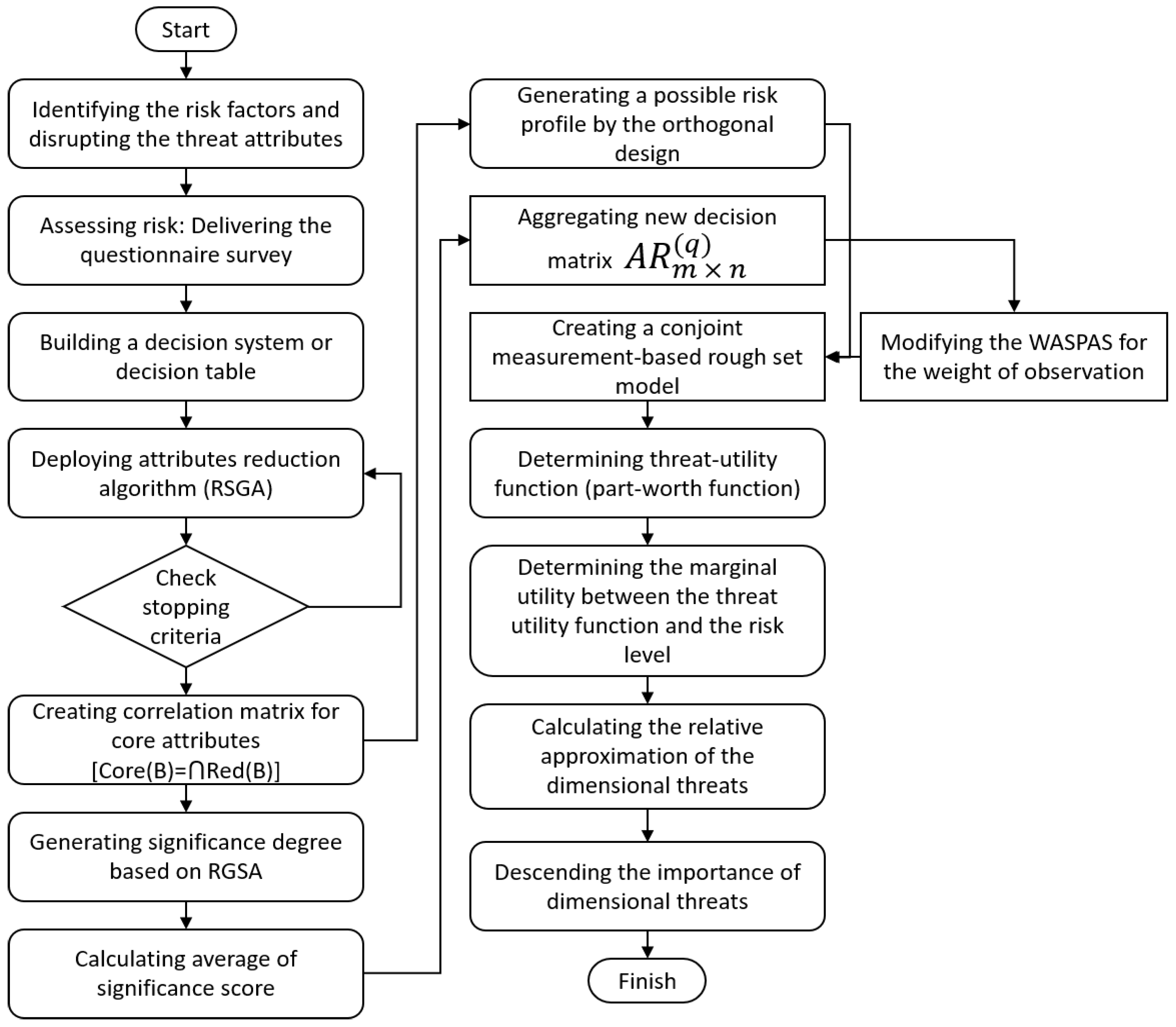
3.3. The Framework of the Threat Utility-Based Hybrid Rough Set Design
3.3.1. Description of Threat Utility Problems
3.3.2. Orthogonal Design
3.3.3. Weight of Observations
3.3.4. Utility Representations Forms
4. An Empirical Analysis of Threat Utility Study
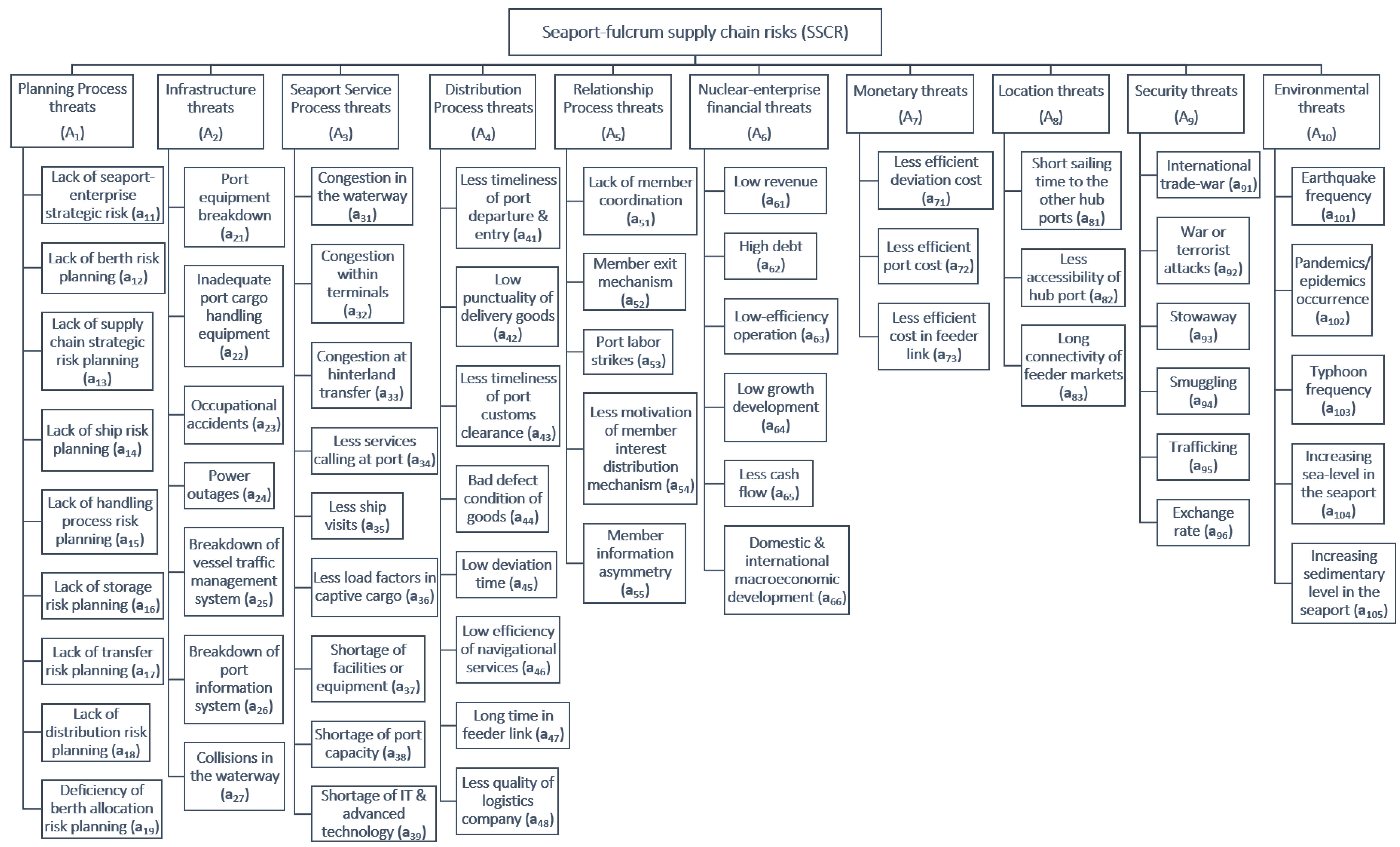
4.1. Data Selection and Coding the Attributes
4.2. Data Collection Procedures
4.3. Reliability Test
4.4. Evaluation of Core Attributes and Orthogonal Design
4.5. Threat Utility of PSCRD
4.5.1. Part-Worth Utility and Its Threat Utility Function
4.5.2. Importance of Dimensional Threats
4.6. Results and Discussion
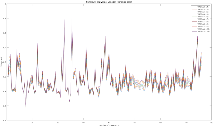
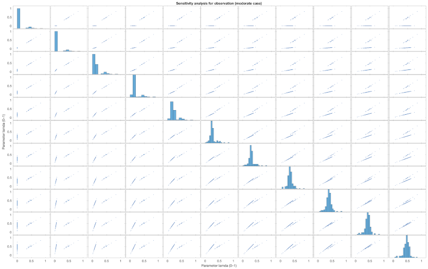
4.7. Sensitivity Analysis
5. Conclusions
Author Contributions
Funding
Institutional Review Board Statement
Informed Consent Statement
Data Availability Statement
Acknowledgments
Conflicts of Interest
Appendix A. Notation (Sets, Indices, Parameters, and Decision Variables)
| ∙ U | : Set of observation, indexed by x ∈ U. |
| ∙ A | : Set of conditional risk factors, indexed by aij ∈ A for all attributes (C and D) |
| ∙Va | : Set of risk magnitude or level for a-th attribute, indexed by f(x,a) ∈ Va |
| ∙ IB or B | : Set of indiscernible relation, indexed by (x1, x2) ∈ IB |
| ∙ i | : Threat factors, i = 1, 2, …, m |
| ∙ j | : Seaport risk factors, j = 1, 2, …, n |
| ∙ J | : Seaport risk profiles aggregated from the q-th expert, J = 1, 2, …, Jq |
| ∙ q | : Number of experts, q = 1, 2, …, l |
| ∙ η | : Expert evaluation in orthogonal design |
| ∙ μ | : Cost criteria normalization |
| ∙ Q | : Ranking set of observation |
| ∙ λ | : Initial criteria accuracy |
| ∙ γ | : Dependency degree |
| ∙ S | : Significant degree |
| ∙p1 | : Classification ability |
| ∙p2 | : Reduction rate |
| ∙p3 | : Correction factor |
| ∙kB | : Dependency degree for each indiscernible relation ai ∈ IB |
| ∙FB | : Attributes reduction set |
| ∙ Λ | : Relative importance of the core attributes |
| ∙ ω | : Average of relative importance |
| ∙ | : Significant degree indicator |
| ∙ DR | : Design range of risk profile |
| ∙Qn | : J − 1 = number of dummy variables for the a-th attribute |
| ∙Dmn | : The dummy variable for the m-th threat dimension of the n-th risk attribute (m = 1, 2, ..., Ma) |
| ∙DmnJ | : Value of the dummy variable, Dmn for the risk profile |
| ∙ Ua(m) | : Utility function for the m-th dimension threat for q-th expert; m = 1, 2, ..., M |
Appendix B. Orthogonal Design of Seaport Risk Combinations (Risk Profile)
| Numbers of Risk Profiles | Threat Factors (Latent Variables) | |||||||||
| A1 | A2 | A3 | A4 | A5 | A6 | A7 | A8 | A9 | A10 | |
| 1. | a18 | a25 | a31 | a42 | a5N | a61 | a7N | a8N | a91 | a101 |
| 2. | a18 | a25 | a39 | a43 | a54 | a64 | a7N | a8N | a91 | a101 |
| 3. | a18 | a26 | a31 | a42 | a5N | a61 | a7N | a81 | a94 | a101 |
| 4. | a14 | a25 | a31 | a42 | a54 | a61 | a73 | a81 | a91 | a101 |
| 5. | a18 | a26 | a33 | a43 | a54 | a61 | a73 | a8N | a91 | a102 |
| 6. | a18 | a26 | a33 | a43 | a54 | a61 | a7N | a81 | a95 | a101 |
| 7. | a16 | a26 | a38 | a42 | a5N | a61 | a73 | a81 | a91 | a101 |
| 8. | a14 | a26 | a31 | a42 | a54 | a61 | a73 | a8N | a95 | a101 |
| 9. | a14 | a26 | a33 | a43 | a5N | a61 | a73 | a8N | a94 | a101 |
| 10. | a15 | a26 | a34 | a43 | a5N | a61 | a7N | a8N | a91 | a101 |
| 11. | a16 | a25 | a31 | a43 | a54 | a61 | a7N | a81 | a91 | a102 |
| 12. | a15 | a26 | a39 | a42 | a54 | a61 | a73 | a81 | a95 | a105 |
| 13. | a16 | a26 | a34 | a43 | a54 | a61 | a73 | a81 | a91 | a101 |
| 14. | a16 | a25 | a33 | a42 | a5N | a61 | a7N | a81 | a91 | a105 |
| 15. | a14 | a26 | a34 | a42 | a54 | a61 | a7N | a81 | a91 | a102 |
| 16. | a14 | a25 | a34 | a42 | a54 | a61 | a7N | a8N | a94 | a105 |
| 17. | a16 | a26 | a31 | a43 | a54 | a61 | a7N | a8N | a95 | a105 |
| 18. | a14 | a25 | a39 | a43 | a5N | a61 | a73 | a81 | a91 | a101 |
| 19. | a15 | a25 | a33 | a42 | a54 | a61 | a73 | a8N | a91 | a102 |
| 20. | a18 | a26 | a34 | a42 | a5N | a61 | a73 | a8N | a91 | a105 |
| 21. | a16 | a25 | a33 | a42 | a5N | a61 | a73 | a8N | a95 | a101 |
| 22. | a16 | a25 | a34 | a43 | a54 | a61 | a73 | a8N | a94 | a101 |
| 23. | a15 | a25 | a33 | a42 | a54 | a61 | a7N | a81 | a94 | a101 |
| 24. | a18 | a25 | a38 | a43 | a54 | a61 | a73 | a81 | a94 | a105 |
| 25. | a15 | a26 | a38 | a42 | a54 | a61 | a7N | a8N | a91 | a101 |
| 26. | a18 | a25 | a34 | a42 | a5N | a61 | a73 | a81 | a95 | a102 |
| 27. | a14 | a25 | a38 | a43 | a5N | a61 | a7N | a8N | a95 | a102 |
| 28. | a15 | a25 | a31 | a43 | a5N | a61 | a73 | a8N | a91 | a105 |
| 29. | a16 | a26 | a39 | a42 | a5N | a61 | a7N | a8N | a94 | a102 |
| 30. | a14 | a26 | a33 | a43 | a5N | a61 | a7N | a81 | a91 | a105 |
| 31. | a15 | a26 | a31 | a43 | a5N | a61 | a73 | a81 | a94 | a102 |
| 32. | a15 | a25 | a34 | a43 | a5N | a61 | a7N | a81 | a95 | a101 |
Appendix C. Variation in Average Criteria

Appendix D. Variation in Cost Criteria
Appendix E. Distribution of Average Criteria
Appendix F. Distribution of Cost Criteria

References
- John, A.; Paraskevadakis, D.; Bury, A.; Yang, Z.; Riahi, R.; Wang, J. An integrated fuzzy risk assessment for seaport operations. Saf. Sci. 2014, 68, 180–194. [Google Scholar] [CrossRef] [Green Version]
- Arisha, A.; Mahfouz, A. Seaport Management Aspects and Perspectives: An Overview. In Proceedings of the 12th Irish Academy of Management Conference, Galway, Ireland, 2–4 September 2009. [Google Scholar] [CrossRef]
- Repetto, M.P.; Burlando, M.; Solari, G.; De Gaetano, P.; Pizzo, M. Integrated tools for improving the resilience of seaports under extreme wind events. Sustain. Cities Soc. 2017, 32, 277–294. [Google Scholar] [CrossRef]
- Ko, W.-C. Construction of house of quality for new product planning: A 2-tuple fuzzy linguistic approach. Comput. Ind. 2015, 73, 117–127. [Google Scholar] [CrossRef]
- Komalasari, D.Y.; Purnamasari, D. Costs of maritime security inspection to merchant ship operations—The Indonesian shipowners’ perspective. Aust. J. Marit. Ocean. Affairs. 2021, 1–16. [Google Scholar] [CrossRef]
- Horck, J. Cultural and Gender Diversities Affecting the Ship/Port Interface. In Proceedings of the First International Ship Port Interface Conference (ISPIC 2008), Bremen, Germany, 19–21 May 2008; Available online: http://bit.ly/2gowXYY (accessed on 7 June 2021).
- Robinson, R. Regulating efficiency into port-oriented chain systems: Export coal through the Dalrymple Bay Terminal, Australia. Marit. Policy Manag. 2007, 34, 89–106. [Google Scholar] [CrossRef]
- Rao, S.; Goldsby, T.J. Supply chain risks: A review and typology. Int. J. Logist. Manag. 2009, 20, 97–123. [Google Scholar] [CrossRef]
- Cavinato, J.L. Supply chain logistics risks: From the back room to the board room. Int. J. Phys. Distrib. Logist. Manag. 2004, 34, 383–387. [Google Scholar] [CrossRef]
- Spekman, R.E.; Davis, E.W. Risky business: Expanding the discussion on risk and the extended enterprise. Int. J. Phys. Distrib. Logist. Manag. 2004, 34, 414–433. [Google Scholar] [CrossRef]
- Ackermann, F.; Howick, S.; Quigley, J.; Walls, L.; Houghton, T. Systemic risk elicitation: Using causal maps to engage stakeholders and build a comprehensive view of risks. Eur. J. Oper. Res. 2014, 238, 290–299. [Google Scholar] [CrossRef]
- Wu, X.; Liao, H. A consensus-based probabilistic linguistic gained and lost dominance score method. Eur. J. Oper. Res. 2019, 272, 1017–1027. [Google Scholar] [CrossRef]
- Kahraman, C.; Çebı, S. A new multi-attribute decision making method: Hierarchical fuzzy axiomatic design. Expert Syst. Appl. 2019, 36, 4848–4861. [Google Scholar] [CrossRef]
- Nguyen, S.; Chen, P.S.-L.; Du, Y. Risk assessment of maritime container shipping blockchain-integrated systems: An analysis of multi-event scenarios. Transp. Res. Part E Logist. Transp. Rev. 2022, 163, 102764. [Google Scholar] [CrossRef]
- Do. Bagus, M.R.; Hanaoka, S. The central tendency of the seaport-fulcrum supply chain risk in Indonesia using a rough set. Asian J. Shipp. Logist. 2022. [Google Scholar] [CrossRef]
- Siswanto, N.; Kurniawati, U.; Latiffianti, E.; Rusdiansyah, A.; Sarker, R. A Simulation study of sea transport based fertilizer product considering disruptive supply and congestion problems. Asian J. Shipp. Logist. 2018, 34, 269–278. [Google Scholar] [CrossRef]
- Jiang, B.; Li, J.; Shen, S. Supply chain risk assessment and control of port enterprises: Qingdao port as case study. Asian J. Shipp. Logist. 2018, 34, 198–208. [Google Scholar] [CrossRef]
- Mennis, E.; Platis, A.; Lagoudis, I.; Nikitakos, N. Improving port container terminal efficiency with the use of Markov theory. Marit. Econ. Logist. 2008, 10, 243–257. [Google Scholar] [CrossRef]
- Gurning, R.O.; Cahoon, S.; Sambodho, K. Supply chain risk management strategies for managing maritime disruptions due to the effects of climate change evidence from the Australian Indonesian wheat supply chain. In Proceedings of the JIWECC, Surabaya, Indonesia, 8–10 August 2010. [Google Scholar]
- Lloyd, C.; Onyeabor, E.; Nwafor, N.; Alozie, O.J.; Nwafor, M.; Mahakweabba, U.; Adibe, E. Maritime transportation and the Nigerian economy: Matters arising. Commonw. Law Bull. 2019, 45, 390–410. [Google Scholar] [CrossRef]
- Loh, H.S.; Thai, V.V.; Wong, Y.D.; Yuen, K.F.; Zhou, Q. Portfolio of port-centric supply chain disruption threats. Int. J. Logist. Manag. 2017, 28, 1368–1386. [Google Scholar] [CrossRef]
- Hassanzadeh, M.A. Port safety: Requirements & economic outcomes. In Marine Navigation and Safety of Sea Transportation: Maritime Transport & Shipping; Weintrit, A., Neumann, T., Eds.; Taylor & Francis Group: Milton Park, UK, 2013. [Google Scholar]
- Kim, K.H.; Lee, H. Container terminal operation: Current trends and future challenges. In International Series in Operations Research & Management Science, 127th ed.; Lee, C.-Y., Meng, Q., Eds.; Springer International Publishing: New York, NY, USA, 2015; pp. 43–73. [Google Scholar]
- Mansouri, M.; Nilchiani, R.; Mostashari, A. A policy making framework for resilient port infrastructure systems. Mar. Policy 2010, 34, 1125–1134. [Google Scholar] [CrossRef]
- Alyami, H.; Lee, P.T.-W.; Yang, Z.; Riahi, R.; Bonsall, S.; Wang, J. An advanced risk analysis approach for container port safety evaluation. Marit. Policy Manag. 2014, 41, 634–650. [Google Scholar] [CrossRef]
- Alyami, H.; Yang, Z.; Riahi, R.; Bonsall, S.; Wang, J. Advanced uncertainty modelling for container port risk analysis. Accid. Anal. Prev. 2016, 123, 411–421. [Google Scholar] [CrossRef] [PubMed]
- Adewole, A. Logistics and supply chain infrastructure development in Africa. In Logistics and Global Value Chains in Africa; Springer International Publishing: Cham, Switzerland, 2019; pp. 17–43. [Google Scholar]
- Na, U.J.; Shinozuka, M. Simulation-based seismic loss estimation of seaport transportation system. Reliab. Eng. Syst. Saf. 2009, 94, 722–731. [Google Scholar] [CrossRef]
- Sudha, M. Evolutionary and neural computing-based decision support system for disease diagnosis from clinical data sets in medical practice. J. Med. Syst. 2017, 41, 178. [Google Scholar] [CrossRef]
- Pawlak, Z. Rough Sets: Theoretical Aspects of Reasoning about Data; Springer: Dordrecht, Switzerland, 1991. [Google Scholar] [CrossRef]
- Luo, K.; Ji, H.; Fu, P.; Tong, X. A New Method Based on Genetic Algorithm for Reduction of Attribution under Incomplete Decision-Making Table. In Proceedings of the Third International Conference on Natural Computation (ICNC), Haikou, China, 24–27 August 2007; pp. 406–410. [Google Scholar] [CrossRef]
- Rao, V.R. Applied Conjoint Analysis; Springer: Berlin/Heidelberg, Germany, 2014. [Google Scholar]
- Zavadskas, E.K.; Antucheviciene, J.; Razavi, H.S.H.; Hashemi, S.S. Extension of weighted aggregated sum product assessment with interval-valued intuitionistic fuzzy numbers (WASPAS-IVIF). Appl. Soft Comput. 2014, 24, 1013–1021. [Google Scholar] [CrossRef]
- Xingli, W.; Liao, H. Utility-based hybrid fuzzy axiomatic design and its application in supply chain finance decision making with credit risk assessments. Comput. Ind. 2020, 114, 103144. [Google Scholar] [CrossRef]
- Kavirathna, C.; Kawasaki, T.; Hanaoka, S.; Matsuda, T. Transshipment hub port selection criteria by shipping lines: The case of hub ports around the Bay of Bengal. J. Shipp. Trade 2018, 3, 4. [Google Scholar] [CrossRef] [Green Version]
- Susanto, T.D.; Diani, M.M.; Hafidz, I. User acceptance of e-government citizen report system (a case study of City113 app). Procedia Comput. Sci. 2017, 124, 560–568. [Google Scholar] [CrossRef]
- Gou, X.; Xu, Z. Managing noncooperative behaviors in large-scale group decision-making with linguistic preference orderings: The application in Internet Venture Capital. Inf. Fusion 2021, 69, 142–155. [Google Scholar] [CrossRef]
- Rahmanto, W.P. Kandangan Dry Port Project: An Option of Solution for Congestion: Case of Lamong Bay Terminal (Surabaya, Indonesia). Master’s Thesis, World Maritime University, Malmö, Sweden, 2016. Available online: https://commons.wmu.se/all_dissertations/528 (accessed on 9 July 2021).


| No. | Seaport Risk Events | Threats to Supply Chain Disruption |
|---|---|---|
| 1. | The interdependency of disrupted events [14,15] | The creation of a domino effect that spread conditional seaport risk and increased the uncertainty of seaport operations resilience. |
| 2. | Organizational planning process [16,17] | Problem of storage planning, particularly in the fertilizer product supply chain Decline in the ship’s utility and increase in its operational cost owing to demurrage in the loading port |
| 3. | Seaport infrastructure breakdown [18,19,21,22] | Decline in the productivity and efficiency of seaport operations Exposure of the cargo to possible hazard and loss Decline in ports’ cost efficiency and a consequential increase in the total transport cost borne by the supply chain parties |
| 4. | Operational inefficiency in terminal [17,21,23] | Impact on the planning of existing infrastructure and resources. Impact on the availability of equipment and workforce |
| 5. | Inadequate cargo handling equipment for hazardous goods [1,24,25,26,27] | Cargo spillages caused by handling hazardous goods or petroleum products Collisions due to the breakdown of cranes or rail-mounted cranes and trailers Increase in the cost of imported goods |
| 6. | Natural disaster effect on the seaport operation [1,2,24,28] | Severe economic losses and social consequences Exposure to operational, environmental, security, technical, and organizational risks |
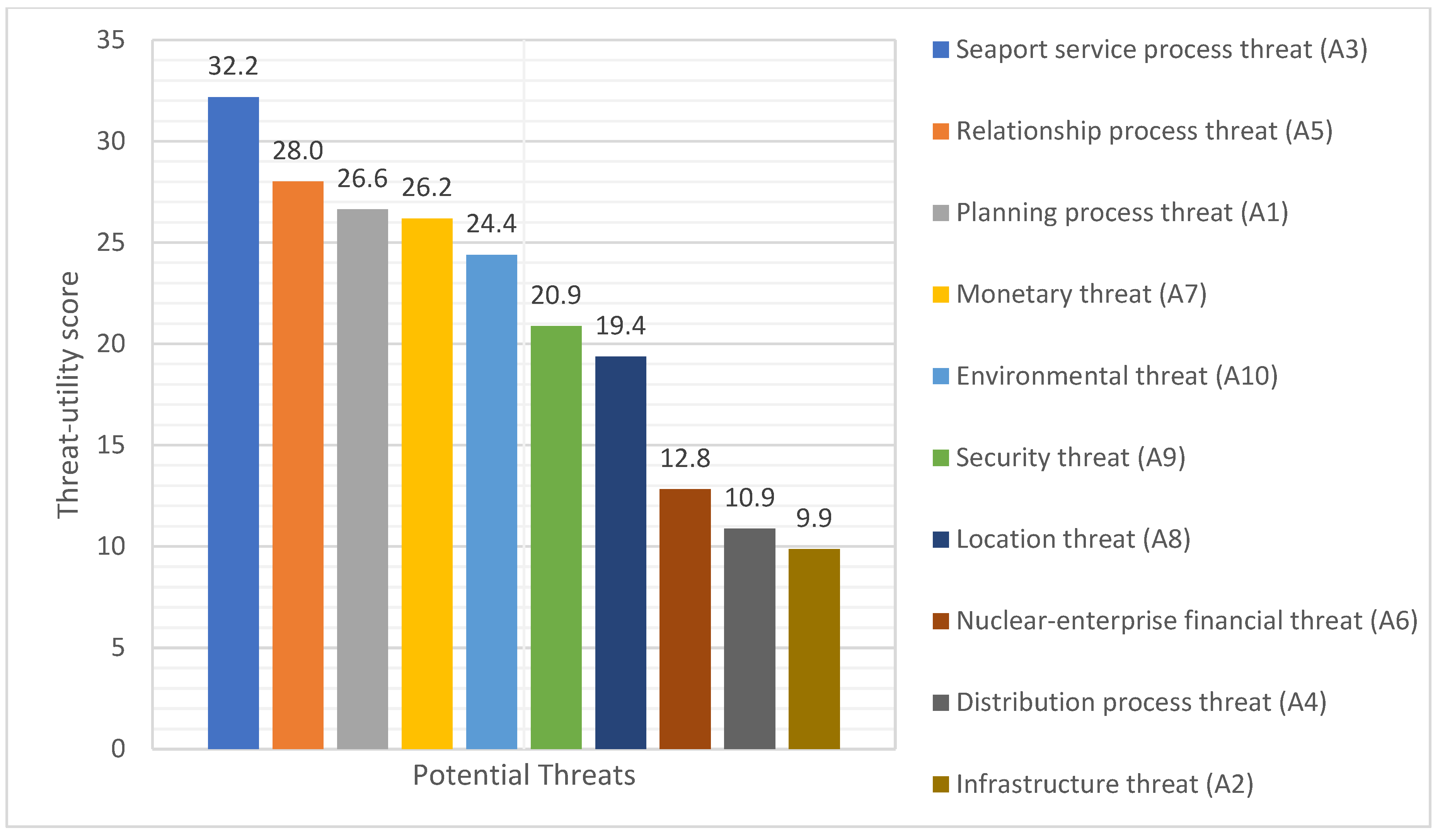
| Dimensional Threats | Definition Scale: Conditional Seaport Risk Evaluation (Code Form) |
|---|---|
| Planning process threat (A1) | Highest level: Loss of ability to perform operations and/or meet customer requirements. High level: Temporary interruption or discontinuity in normal operations, delivery of goods, and/or services to customers. Medium level: Postponement in regular operations, plans and schedules, conveyance of products, and/or service to customers. Low level: Deviation in transportation plans, costs, common operations, timetables, quality, measure of conveyed merchandise (product), and/or services to customers. Lowest level: Operations remain unaffected or experience a negligible effect |
| Infrastructure threat (A2) | |
| Seaport service process threat (A3) | |
| Distribution process threat (A4) | |
| Relationship process threat (A5) | |
| Nuclear-enterprise financial threat (A6) | |
| Monetary threat (A7) | |
| Location threat (A8) | |
| Security threat (A9) | |
| Environmental threat (A10) |
| No. | Demographic Factor | Percentage | |
|---|---|---|---|
| 1. | Gender | Male | 70% |
| Female | 30% | ||
| 2. | Object of research | Seaport manager | 11% |
| Seaport operator | 43% | ||
| Seaport user | 47% | ||
| 3. | Work duration | Below 5 years | 4% |
| Between 5–10 years | 39% | ||
| Over 10 years | 57% | ||
| 4. | Educational background | Diploma | 10% |
| Bachelor | 61% | ||
| Master’s | 27% | ||
| Doctoral | 2% | ||
| Case Processing Summary | Number of Responses | Percentage | |
|---|---|---|---|
| Cases | Valid | 153 | 100% |
| Excluded a | 0 | 0.0 | |
| Total | 153 | 100% | |
| Reliability results for questionnaire survey | |||
| Cronbach’s alpha | 0.882 | 88.2% | |
| Number of features | 62 | 100% | |
| Reliability results for the aggregation of seaport risk alternative | |||
| Cronbach’s alpha | 0.991 | 99.1% | |
| Cronbach’s alpha based on standardized items | 0.992 | 99.2% | |
| Number of features | 32 | 100% | |
| No. | Dimensional Threats | Attributes | ||
|---|---|---|---|---|
| 1 | Planning Process threat (A1) | a14 | 0.023 | 0.048 |
| 2 | a15 | 0.021 | 0.042 | |
| 3 | a16 | 0.015 | 0.031 | |
| 4 | a18 | 0.014 | 0.029 | |
| 5 | Infrastructure threat (A2) | a25 | 0.073 | 0.149 |
| 6 | a26 | 0.019 | 0.038 | |
| 7 | Seaport Service Process threat (A3) | a31 | 0.018 | 0.038 |
| 8 | a33 | 0.037 | 0.076 | |
| 9 | a34 | 0.014 | 0.028 | |
| 10 | a38 | 0.016 | 0.033 | |
| 11 | a39 | 0.025 | 0.050 | |
| 12 | Distribution Process threat (A4) | a42 | 0.015 | 0.030 |
| 13 | a43 | 0.023 | 0.046 | |
| 14 | Relationship Process threat (A5) | a54 | 0.092 | 0.188 |
| 15 | Nuclear-enterprise financial threat (A6) | a61 | 0.015 | 0.031 |
| 16 | a64 | 0.020 | 0.041 | |
| 17 | Monetary threat (A7) | a73 | 0.035 | 0.072 |
| 18 | Location threat (A8) | a81 | 0.022 | 0.045 |
| 19 | Security threat (A9) | a91 | 0.022 | 0.044 |
| 20 | a94 | 0.021 | 0.043 | |
| 21 | a95 | 0.043 | 0.087 | |
| 22 | Environmental threat (A10) | a101 | 0.021 | 0.043 |
| 23 | a102 | 0.032 | 0.066 | |
| 24 | a105 | 0.020 | 0.041 |
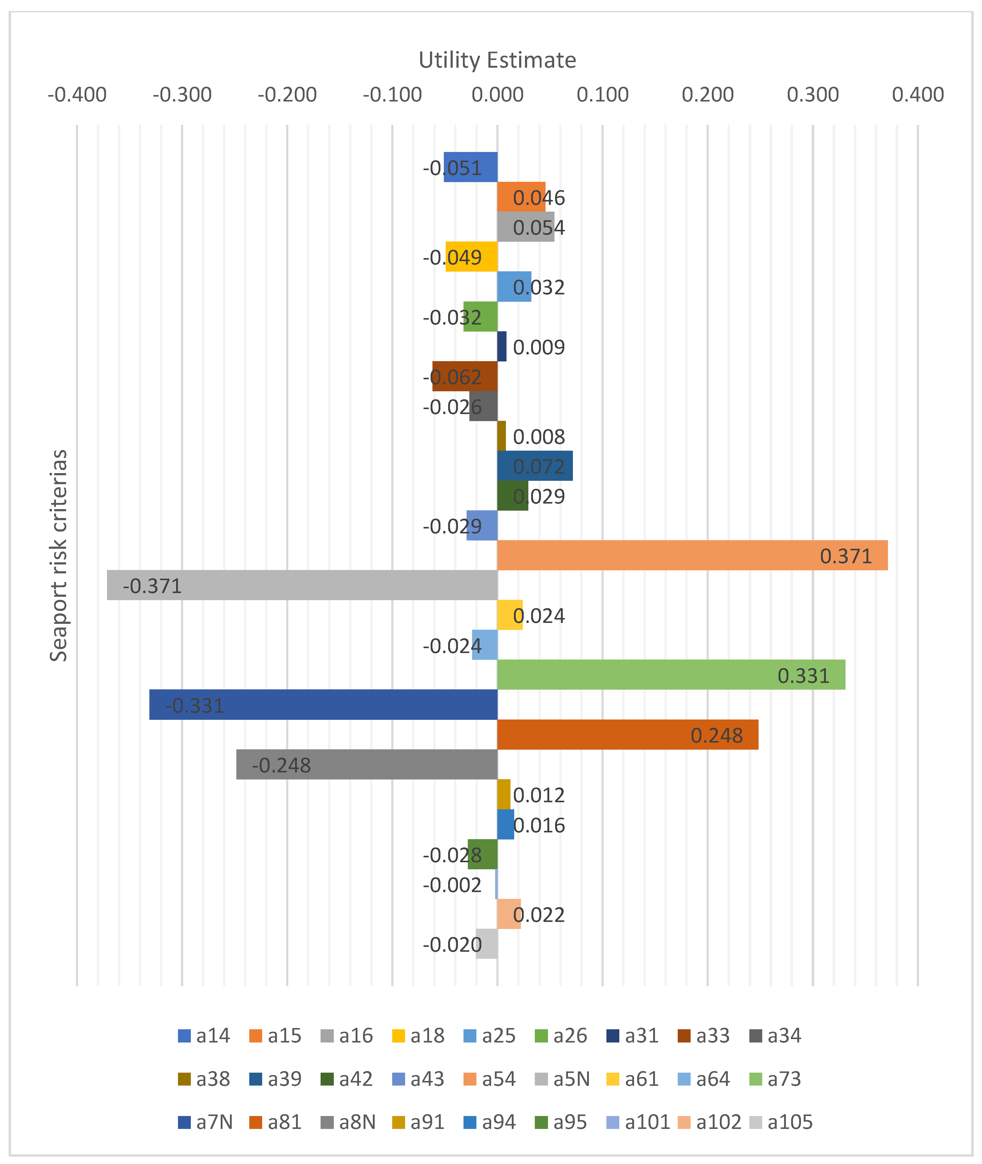
| No. | Threat Variables | Part-Worth (Partial) Utility Function |
|---|---|---|
| 1. | Planning process threat (A1) | U(A1) = −0.051a14+ 0.046a15 + 0.054a16 − 0.049a18 |
| 2. | Infrastructure threat (A2) | U(A2) = 0.032a25− 0.032a26 |
| 3. | Seaport service process threat (A3) | U(A3) = 0.009a31− 0.062a33 − 0.026a34 + 0.008a38 + 0.072a39 |
| 4. | Distribution process threat (A4) | U(A4) = 0.029a42− 0.029a43 |
| 5. | Relationship process threat (A5) | U(A5) = 0.371a54− 0.371a5N |
| 6. | Nuclear-enterprise financial threat (A6) | U(A6) = 0.024a61− 0.024a64 |
| 7. | Monetary threat (A7) | U(A7) = 0.331a73− 0.331a7N |
| 8. | Location threat (A8) | U(A8) = 0.248a81− 0.248a8N |
| 9. | Security threat (A9) | U(A9) = 0.012a91+ 0.016a94 − 0.028a95 |
| 10. | Environmental threat (A10) | U(A10) = −0.002a101+ 0.022a102 − 0.02a105 |
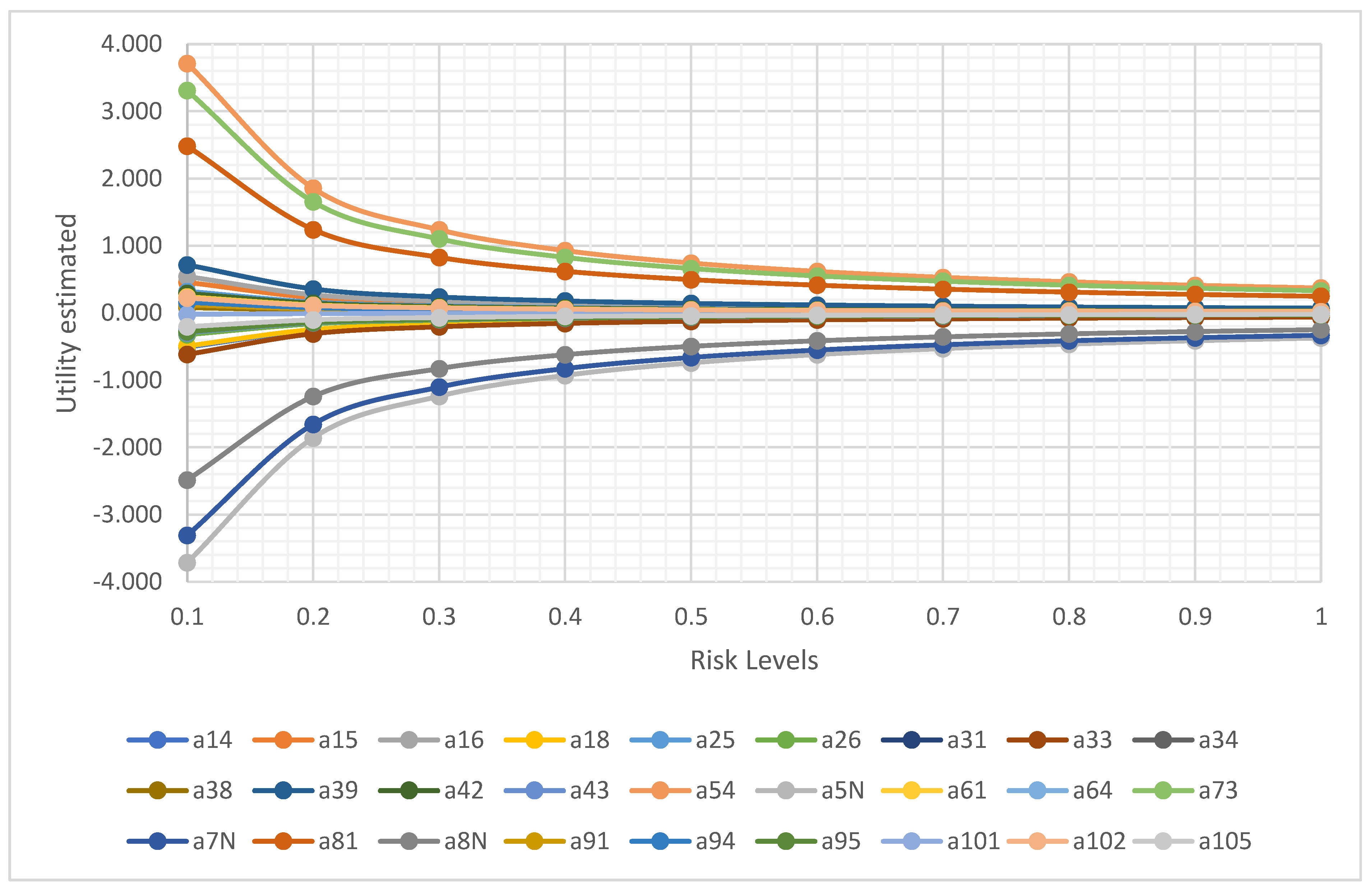
| Risk Factors | Estimated Utility | ||||||
|---|---|---|---|---|---|---|---|
| Overall | e1 | e2 | e3 | e4 | ~ | e153 | |
| Constant | 1.33 | 0.104 | 0.162 | 0.082 | 0.035 | ~ | 0.137 |
| a14 | −0.05 | 0.155 | 0.242 | 0.123 | 0.052 | ~ | 0.204 |
| a15 | 0.05 | 0.155 | 0.242 | 0.123 | 0.052 | ~ | 0.204 |
| a16 | 0.05 | 0.155 | 0.242 | 0.123 | 0.052 | ~ | 0.204 |
| a18 | −0.05 | 0.155 | 0.242 | 0.123 | 0.052 | ~ | 0.204 |
| a25 | 0.03 | 0.090 | 0.140 | 0.071 | 0.030 | ~ | 0.118 |
| a26 | −0.03 | 0.090 | 0.140 | 0.071 | 0.030 | ~ | 0.118 |
| a31 | 0.01 | 0.168 | 0.262 | 0.133 | 0.056 | ~ | 0.221 |
| a33 | −0.06 | 0.168 | 0.262 | 0.133 | 0.056 | ~ | 0.221 |
| a34 | −0.03 | 0.168 | 0.262 | 0.133 | 0.056 | ~ | 0.221 |
| a38 | 0.01 | 0.218 | 0.340 | 0.173 | 0.073 | ~ | 0.287 |
| a39 | 0.07 | 0.218 | 0.340 | 0.173 | 0.073 | ~ | 0.287 |
| a42 | 0.03 | 0.090 | 0.140 | 0.071 | 0.030 | ~ | 0.118 |
| a43 | −0.03 | 0.090 | 0.140 | 0.071 | 0.030 | ~ | 0.118 |
| a54 | 0.37 | 0.090 | 0.140 | 0.071 | 0.030 | ~ | 0.118 |
| a5N | −0.37 | 0.090 | 0.140 | 0.071 | 0.030 | ~ | 0.118 |
| a61 | 0.02 | 0.090 | 0.140 | 0.071 | 0.030 | ~ | 0.118 |
| a64 | −0.02 | 0.090 | 0.140 | 0.071 | 0.030 | ~ | 0.118 |
| a73 | 0.33 | 0.090 | 0.140 | 0.071 | 0.030 | ~ | 0.118 |
| a7N | −0.33 | 0.090 | 0.140 | 0.071 | 0.030 | ~ | 0.118 |
| a81 | 0.25 | 0.090 | 0.140 | 0.071 | 0.030 | ~ | 0.118 |
| a8N | −0.25 | 0.090 | 0.140 | 0.071 | 0.030 | ~ | 0.118 |
| a91 | 0.01 | 0.120 | 0.186 | 0.095 | 0.040 | ~ | 0.157 |
| a94 | 0.02 | 0.140 | 0.219 | 0.111 | 0.047 | ~ | 0.184 |
| a95 | −0.03 | 0.140 | 0.219 | 0.111 | 0.047 | ~ | 0.184 |
| a101 | 0.00 | 0.120 | 0.186 | 0.095 | 0.040 | ~ | 0.157 |
| a102 | 0.02 | 0.140 | 0.219 | 0.111 | 0.047 | ~ | 0.184 |
| a105 | −0.02 | 0.140 | 0.219 | 0.111 | 0.047 | ~ | 0.184 |
| R2 coefficients | 1.00 | 0.705 | 0.766 | 0.899 | 0.756 | ~ | 0.769 |
Publisher’s Note: MDPI stays neutral with regard to jurisdictional claims in published maps and institutional affiliations. |
© 2022 by the authors. Licensee MDPI, Basel, Switzerland. This article is an open access article distributed under the terms and conditions of the Creative Commons Attribution (CC BY) license (https://creativecommons.org/licenses/by/4.0/).
Share and Cite
Do Bagus, M.R.; Hanaoka, S. Threat Utility of the Seaport Risk Factors: Use of Rough Set-Based Genetic Algorithm. J. Mar. Sci. Eng. 2022, 10, 1484. https://doi.org/10.3390/jmse10101484
Do Bagus MR, Hanaoka S. Threat Utility of the Seaport Risk Factors: Use of Rough Set-Based Genetic Algorithm. Journal of Marine Science and Engineering. 2022; 10(10):1484. https://doi.org/10.3390/jmse10101484
Chicago/Turabian StyleDo Bagus, Muhammad Reza, and Shinya Hanaoka. 2022. "Threat Utility of the Seaport Risk Factors: Use of Rough Set-Based Genetic Algorithm" Journal of Marine Science and Engineering 10, no. 10: 1484. https://doi.org/10.3390/jmse10101484
APA StyleDo Bagus, M. R., & Hanaoka, S. (2022). Threat Utility of the Seaport Risk Factors: Use of Rough Set-Based Genetic Algorithm. Journal of Marine Science and Engineering, 10(10), 1484. https://doi.org/10.3390/jmse10101484