Wave Boundary Layer at the Ice–Water Interface

Abstract

On re-examining the problem of linear gravity waves in two layers of fluids with a viscous ice layer overlaying water of deep depth, we give a detailed analysis of the fluid velocities, velocity shear, and Reynolds stress associated with wave fluctuations in both the ice layer and the wave boundary layer just beneath it. For the turbulent wave boundary layer, water eddy viscosity is used. Comprehensive discussions on various aspects of the velocity fields are made in terms of a Reynolds number based on the ice-layer thickness and viscosity, and the ice-to-water viscosity ratio. Speculation of the wave-induced steady streaming is made based on the Reynolds stress distribution, offering a preliminary insight into the mean flows in both the ice layer and wave boundary layer in the water. For wave attenuation, the results using a typical ice viscosity and a reasonable water eddy viscosity show good agreement with data over the range of frequencies for field and lab waves, significantly outperforming those assuming an inviscid water.

1. Introduction

Marginal ice zones (MIZs) are distinguished by the highly heterogeneous condition of sea ice, e.g., floes of various sizes, pancake, brash and frazil ice, ice ages, brine content, ice thickness and concentration, etc. This makes it challenging to model wave propagation in MIZs, either theoretically or numerically, since there remain similar limitations to mathematically describing such an ice cover on the ocean surface. Even with today’s computing resources, it is intimidating to discretely model individual sea ice interacting with random waves as they propagate in the MIZ.

Aiming at describing the collective effects of broken ice, mathematical models tend to treat such a heterogeneous ice cover as a continuum, e.g., the mass loading model [1], models of elastic plates or viscoelastic beams [2,3,4], and models of two layers of fluids with a viscous or viscoelastic ice layer overlaying water [5,6,7,8,9,10], among others; see reviews in [11,12]. In most of those studies, the primary interest is to obtain the dispersion equation, which describes the relation between the wave frequency $\omega =2\pi /f$ and complex wavenumber $k=k_r+\mathrm{i}{k}_i$, where $2\pi /k_r$ is the wavelength and $k_i$ is the wave attenuation rate (if the system is dissipative). The intense interest is driven, in part, by applications of large-scale modeling of waves in MIZs, where a reliable estimate of $k_i\left(\omega \right)$ is important since it enters the formulation of model dynamics for wave energy spectral distribution [13].

Despite the complexities in various treatments of the ice-agglomeration layer, many existing studies assume an inviscid underlying water, with a few exceptions (e.g., [5,7,9]). Furthermore, the emphasis on wave attenuation seems to have overshadowed interest in other aspects of the linear wave motions in ice-covered water. In most abovementioned studies, features of the velocity fields in both the ice layer and the water beneath it are little discussed. For a composite, dissipative fluid system, such as a viscous or viscoelastic ice layer overlaying water, the velocity distributions in both fluids are not definitely determined until the dispersion relationship is solved. In the mathematical forms of the wave-like solutions, there is a set of coefficients that specify the contributions of rotational (due to the presence of viscosities) and irrotational flows in a layer, and the proportionality between flows in different layers. These coefficients are not individually arbitrary, but have a relationship that is constrained by the conditions at the uppermost free surface and the fluid–fluid interface(s), and is unique to a given wave frequency. This is seen more clearly from the mathematical point of view. Regardless of the different physics in modeling the ice layer and whether the water is viscous or inviscid, the mathematical problem of this type of linear wave theory is eventually to solve a homogeneous system (in matrix form Mx = 0) that results from satisfying the free surface boundary and interface conditions. The equation for the wave dispersion relation is the vanishing of the determinant of matrix M, while the admissible values for those abovementioned coefficients are from the null vector x corresponding to $k\left(\omega \right)$. That is, the partitions of the linear flow between the layers, and the rotational and irrotational parts in a layer, are unique for a wave condition of $\omega$ and k, and affected by the fluid properties just as the dispersion relation is.

In this study, we re-consider the problem of linear waves in a two-layer fluid system of a viscous ice layer overlaying viscous water. Our interest is in the distributions of fluid velocities in both the ice layer and wave boundary layer in the water just underneath the ice. With an ice-agglomeration cover, the wave boundary layer at the ice–water interface is expected to be enhanced due to the eddy activities resulting from broken ice interacting with the wave [5,7]. In a recent small-scale lab study, Rabault et al. [14] reported eddy structures from PIV (particle image velocimetry) measurements, attributing their origin to the generation, and subsequent diffusion of strong vortices by the drifting and colliding of packs of grease ice. On the other hand, the water velocities and their shear rates in the boundary layer affect the ice-layer flow above, because of the conditions of stresses and velocities at the ice–water interface. Naturally, questions may be asked: How do the ice-layer viscosity and thickness affect the boundary layer water flow just underneath the ice? How do the eddies and shear-induced mixing in the wave boundary layer, as indicated by the water eddy viscosity, affect the velocity distribution in the ice layer? Furthermore, the effects of viscosities alter the phase relation between the waves on the upper surface and at the interface and, consequently, the phase relation between the fluid velocities. This is the manifestation of waves becoming rotational. However, the physical importance is that the horizontal and vertical velocities of the linear flow are now correlated, producing a Reynolds stress that represents the mean momentum flux due to the linear wave fluctuations. This is the driving force for wave-induced Eulerian steady streaming, which, when combined with the Stokes drift, gives the Lagrangian transport of particles [15,16]. What are the vertical profiles of the wave-induced Reynolds stress in the ice layer and the water underneath it? How are they affected by the ice and water viscosities? With a goal of obtaining the drift velocity under the ice, Weber [5] formulated a nonlinear analysis using a Lagrangian formulation. To ease the mathematical complexity, Weber considered the asymptotic limit when the upper ice layer is so thin and viscous that it is equivalent to an inextensible surface film. While a formal nonlinear analysis can be carried out using the similar method, but treating the ice layer as a viscous fluid, the Reynolds stress (a nonlinear property obtained from the linear flow) can nevertheless provide preliminary insight into the steady streaming.

Since it must first be solved before analyzing the fluid velocity field, we will discuss the results of the dispersion relation, but in the dimensionless plane using the ice thickness-based normalization introduced in [17]. This leads to the dimensionless parameters, including a Reynolds number that is defined using the ice-layer viscosity and thickness, and measures the time scale of vorticity diffusion in the ice-layer flow relative to the inertial time scale of wave motion, the ice-to-water viscosity ratio, and the density ratio. As demonstrated in [17], examination of results in the dimensionless plane leads to more comprehensive understanding. We note that De Carolis and Desiderio [7] formulated the linear wave theory for a viscous ice layer covering viscous water of an arbitrary depth (including deep water depth), but only solved the dispersion relation; when discussing the results (in the dimensional plane) for low frequencies that are relevant for field waves, they limited their attention to very thin ice (1∼3 cm) and high ice viscosity (1∼2000 m${}^2$/s).

Using data from various field and lab studies, Yu et al. [17] calibrated the two-layer models of wave attenuation by sea ice (with underlaying inviscid water) and showed that for the model of a viscoelastic ice, the effective shear modulus needs to be low, between tens to a few hundred Pascal. This suggests that elasticity is not important for broken ice. The analysis in this study is for a viscous ice layer, but can readily be extended to a viscoelastic ice layer with a viscous water if the interest arises. For linear harmonic oscillations in viscoelastic fluids, the Voigt model can be used (i.e., introducing a complex viscosity with the imaginary part incorporating the elasticity) to render the mathematical formulation formally the same as that for viscous fluids. The results here can then be transformed by replacing the ice viscosity with the complex ice viscosity to analyze the linear boundary layer beneath a viscoelastic ice-agglomeration fluid layer. Note that the dispersion relation for such a viscoelastic fluid layer with a viscous water has been studied in [9]. It should be mentioned that there are studies considering the ice cover as an elastic or viscoelastic plate (i.e., a solid) responding to wave motions (e.g., [18,19,20]). The mathematical formulation for floating body–fluid interaction is different from that for a viscoelastic fluid overlaying the water as mentioned above.

The rest of the paper is organized as follows. The mathematical formulation is described in Section 2. Since the equations and solution procedure are standard and can easily be found in the literature, we have purposely omitted the tedious algebraic details to focus on discussing the results in Section 3. The dispersion relation is discussed in Section 3.1; the solution of wave attenuation is compared with a number of field and lab datasets in Section 3.2; the distributions of fluid velocities are analyzed in Section 3.3; the wave-induced Reynold stress is discussed in Section 3.4, where speculation on the steady streaming is also made. Summary and concluding remarks follow in Section 4.

2. Mathematical Formulation

Consider a two-layer fluid system in which the upper layer is thin and highly viscous, representing the ice-agglomeration cover of the ocean surface (Figure 1). Let z points upward and x point to the direction of wave propagation. The undisturbed upper layer occupies $0<z<h$, having a constant density ${\rho }_1$ and an effective ice viscosity ${\nu }_1$. For $z<0$, the seawater density is ${\rho }_2$. Because of the large velocity shear resulting from the interaction with the viscous flow in the ice layer, the seawater viscosity ${\nu }_2$ is expected to be important in the thin wave boundary layer (WBL) at the interface. The thickness of the WBL is $O\left({\delta }_2\right)$, where the Stokes layer thickness in water is ${\delta }_2=\sqrt{2{\nu }_2/\omega }$ and $\omega$ is the angular frequency of the wave. Outside the WBL for $z\ll -{\delta }_2$, the wave motion is approximately inviscid, and the region is referred to as the inviscid core. Without losing any generality and for mathematical simplicity, we consider the water depth to be so deep that the seabed has little effect on the wave at the interface or on the upper surface, and is therefore irrelevant.

Both fluids are considered incompressible, and ${\rho }_1<{\rho }_2$, ${\nu }_1>{\nu }_2$. In the ice layer and WBL in water, the motions are described by the Navier–Stokes equations, while for $z\ll -{\delta }_2$, the Euler equations apply. At the basic state, the fluids are at rest; hence, the pressure is hydrostatic and the free surface of the upper layer and the ice–water interface are horizontal at $z=h$ and $z=0$, respectively. For linear waves, the equations of motion, the boundary conditions at the upper free surface, and the matching conditions at the interface are all linearized about the basic state. Let the subscript j indicate the fluid layer; i.e., $j=1$ for $h<z<0$ in the upper ice layer and $j=2$ for $z<0$ in the water. The continuity equations for mass conservation in both fluids are

$$\frac{\partial u_j}{\partial x}+\frac{\partial v_j}{\partial z}=0.$$

(1)

For the ice-layer and WBL flows, the linearized momentum equations are

$$\frac{\partial {\mathit{u}}_j}{\partial t}=-\frac{1}{{\rho }_j}\nabla P_j+{\nu }_j\left(\frac{{\partial }^2{\mathit{u}}_j}{\partial x^2}+\frac{{\partial }^2{\mathit{u}}_j}{\partial z^2}\right),$$

(2)

where the velocity vector ${\mathit{u}}_j=(u_j,v_j)$ and $P_j$ is the dynamic pressure so that the total pressure

$$\begin{array}{ccc}\hfill p_1& =\hfill & \hfill -{\rho }_{1}g(z-h)+P_1\mathrm{for}0<z<h,\end{array}$$

(3a)

$$\begin{array}{ccc}\hfill p_2& =\hfill & \hfill {\rho }_{1}gh-{\rho }_{2}gz+P_2\mathrm{for}z<0.\end{array}$$

(3b)

Outside the WBL for $z\ll -{\delta }_2$, the motion approaches the inviscid flow that follows

$$\frac{\partial {\mathit{U}}_{\mathrm{I}}}{\partial t}=-\frac{1}{{\rho }_2}\nabla P_{\mathrm{I}},$$

(4)

where ${\mathit{U}}_{\mathrm{I}}=(U_{\mathrm{I}},V_{\mathrm{I}})$ and $P_{\mathrm{I}}$ is the dynamic pressure for the potential flow. ${\eta }_1(x,t)$ and ${\eta }_2(x,t)$ are, respectively, the waves propagating on the upper free surface and at the interface. The linearized boundary conditions at the upper free surface are the kinematic condition, and vanishing of the two components of surface stress, i.e., at $z=h$,

$$\begin{array}{ccc}\hfill \frac{\partial {\eta }_1}{\partial t}& =& v_1,\hfill \end{array}$$

(5)

$$\begin{array}{ccc}\hfill {\nu }_1\left(\frac{\partial u_1}{\partial z}+\frac{\partial v_1}{\partial x}\right)& =& 0,\hfill \end{array}$$

(6)

$$\begin{array}{ccc}\hfill -g{\eta }_1+\frac{P_1}{{\rho }_1}-2{\nu }_1\frac{\partial v_1}{\partial z}& =& 0.\hfill \end{array}$$

(7)

At the interface, the continuity of velocities and stresses are required, i.e., at $z=0$,

$$\begin{array}{ccc}\hfill u_1& =& u_2,\hfill \end{array}$$

(8)

$$\begin{array}{ccc}\hfill v_1& =& v_2=\frac{\partial {\eta }_2}{\partial t},\hfill \end{array}$$

(9)

$$\begin{array}{ccc}\hfill {\rho }_1{\nu }_1\left(\frac{\partial u_1}{\partial z}+\frac{\partial v_1}{\partial x}\right)& =& {\rho }_2{\nu }_2\left(\frac{\partial u_2}{\partial z}+\frac{\partial v_2}{\partial x}\right),\hfill \end{array}$$

(10)

$$\begin{array}{ccc}\hfill P_1-{\rho }_{1}g{\eta }_2-2{\rho }_1{\nu }_1\frac{\partial v_1}{\partial z}& =& P_2-{\rho }_{2}g{\eta }_2-2{\rho }_2{\nu }_2\frac{\partial v_2}{\partial z}.\hfill \end{array}$$

(11)

For $z\ll -{\delta }_2$,

$$(u_2,v_2)\to (U_{\mathrm{I}},V_{\mathrm{I}}),P_2\to P_{\mathrm{I}}.$$

(12)

We consider plane waves propagating in the $+x$ direction on the free surface and at the ice–water interface, and seek solutions in the form of

$$[u_j,v_j,P_j,{\eta }_j]=[{\widehat{u}}_j\left(z\right),{\widehat{v}}_j\left(z\right),{\widehat{P}}_j\left(z\right),{\widehat{\eta }}_j]{\mathrm{e}}^{\mathrm{i}(kx-\omega t)}+\mathrm{c}.\mathrm{c}.,$$

(13)

where the complex wavenumber $k=k_r+\mathrm{i}{k}_i$, $\omega$ is real, and $\mathrm{c}.\mathrm{c}.$ stands for the complex conjugate. The linear Navier–Stokes Equations (1) and (2) can be solved by decomposing the velocity field into the irrotational and rotational components, which can be expressed, respectively, as the gradient of velocity potential and the curl of the stream function [21]. From Equations (1) and (2), we then obtain the Laplacian equation for the velocity potential, the linear vorticity equation for the stream function, and the Bernoulli equation for the pressure field. From those equations, it follows the mathematical forms for the z-dependencies in Equation (13). The algebraic details can be found in the literature (e.g., [7,21]) and are therefore omitted here. We only quote the solution forms. For $0<z<h$,

$$\begin{array}{ccc}\hfill {\widehat{u}}_1& =\hfill & \hfill -\mathrm{i}k(A{\mathrm{e}}^{kz}+B{\mathrm{e}}^{-kz})-{\alpha }_1(C{\mathrm{e}}^{{\alpha }_{1}z}-D{\mathrm{e}}^{-{\alpha }_{1}z}),\end{array}$$

(14a)

$$\begin{array}{ccc}\hfill {\widehat{v}}_1& =\hfill & \hfill -k(A{\mathrm{e}}^{kz}-B{\mathrm{e}}^{-kz})+\mathrm{i}k(C{\mathrm{e}}^{{\alpha }_{1}z}+D{\mathrm{e}}^{-{\alpha }_{1}z}),\end{array}$$

(14b)

$$\begin{array}{ccc}\hfill {\widehat{P}}_1& =\hfill & \hfill -\mathrm{i}\omega {\rho }_1(A{\mathrm{e}}^{kz}+B{\mathrm{e}}^{-kz}),\end{array}$$

(14c)

where

$${\alpha }_1=\sqrt{k^2-\mathrm{i}\omega /{\nu }_1}.$$

(15)

For $z<0$ and inside the WBL, i.e., $-z\sim O\left({\delta }_2\right)$,

$$\begin{array}{ccc}\hfill {\widehat{u}}_2& =\hfill & \hfill -\mathrm{i}kE{\mathrm{e}}^{kz}-{\alpha }_{2}F{\mathrm{e}}^{{\alpha }_{2}z},\end{array}$$

(16a)

$$\begin{array}{ccc}\hfill {\widehat{v}}_2& =\hfill & \hfill -kE{\mathrm{e}}^{kz}+\mathrm{i}kF{\mathrm{e}}^{{\alpha }_{2}z},\end{array}$$

(16b)

$$\begin{array}{ccc}\hfill {\widehat{P}}_2& =\hfill & \hfill -\mathrm{i}\omega {\rho }_{2}E{\mathrm{e}}^{kz},\end{array}$$

(16c)

where

$${\alpha }_2=\sqrt{k^2-\mathrm{i}\omega /{\nu }_2}.$$

(17)

The constant coefficients $A,B,C,D,E,F$ are to be determined. By definition, the real parts of ${\alpha }_1$ and ${\alpha }_2$ are positive. In Equations (14) and (16), the terms associated with ${\alpha }_1$ and ${\alpha }_2$ represent the rotational components of the velocity fields, being associated with the curls of stream functions in the ice layer and WBL, respectively. Note that we can rewrite ${\alpha }_2={\left(k^2-2\mathrm{i}{\delta }_2^{-2}\right)}^{1/2}$. For water wave motions, the eddy viscosity due to turbulent mixing can be as much as 100 cm${}^2$/s or even larger, and 20–40 cm${}^2$/s is the typical range [16]. For a period of 10 s, ${\delta }_2$ can be estimated to be roughly 8–18 cm for a turbulent WBL, compared with the wavelength of 156 m. Thus, $|{\alpha }_2|\sim \sqrt{2}/{\delta }_2$ for most waves. It is then seen from Equation (16) that the terms ${\mathrm{e}}^{{\alpha }_{2}z}$ rapidly die out as we move downward away from $z=0$. Thus, we obtain the potential flow solution in the inviscid core, i.e., for $z\ll -{\delta }_2$,

$${\widehat{U}}_{\mathrm{I}}=-\mathrm{i}kE{\mathrm{e}}^{kz},{\widehat{V}}_{\mathrm{I}}=-kE{\mathrm{e}}^{kz},{\widehat{P}}_{\mathrm{I}}=-\mathrm{i}\omega {\rho }_{2}E{\mathrm{e}}^{kz}.$$

(18)

One can verify that the wave-like solutions in Equation (13), together with Equations (14), (16), and (18), satisfy the continuity Equation (1), the momentum Equation (2) for the viscous flow, and (4) for the potential flow. Upon satisfying the boundary and interface conditions (5)–(11), and substituting the complex amplitudes ${\widehat{\eta }}_1$ and ${\widehat{\eta }}_2$ using (5) and (9), we obtain six homogenous equations for $A,B,C,D,E,F$; i.e.,

$$\begin{array}{ccc}\hfill 2\mathrm{i}{k}^2{\mathrm{e}}^{kh}A-2\mathrm{i}{k}^2{\mathrm{e}}^{-kh}B+({\alpha }_1^2+k^2){\mathrm{e}}^{{\alpha }_{1}h}C+({\alpha }_1^2+k^2){\mathrm{e}}^{-{\alpha }_{1}h}D& =\hfill & \hfill 0,\\ \hfill (2{\nu }_1{k}^2-\mathrm{i}\omega +\mathrm{i}gk/\omega ){\mathrm{e}}^{kh}A+(2{\nu }_1{k}^2-\mathrm{i}\omega -\mathrm{i}gk/\omega ){\mathrm{e}}^{-kh}B& & \hfill \end{array}$$

(19a)

$$\begin{array}{ccc}\hfill -(2\mathrm{i}{\nu }_{1}k{\alpha }_1-gk/\omega ){\mathrm{e}}^{{\alpha }_{1}h}C+(2\mathrm{i}{\nu }_{1}k{\alpha }_1+gk/\omega ){\mathrm{e}}^{-{\alpha }_{1}h}D& =\hfill & \hfill 0,\end{array}$$

(19b)

$$\begin{array}{ccc}\hfill \mathrm{i}kA+\mathrm{i}kB+{\alpha }_{1}C-{\alpha }_{1}D-\mathrm{i}kE-{\alpha }_{2}F& =\hfill & \hfill 0,\end{array}$$

(19c)

$$\begin{array}{ccc}\hfill A-B-\mathrm{i}C-\mathrm{i}D-E+\mathrm{i}F& =\hfill & \hfill 0,\end{array}$$

(19d)

$$\begin{array}{ccc}\hfill \mathrm{i}{k}^2\left(2-\frac{{\rho }_2}{{\rho }_1}\frac{{\nu }_2}{{\nu }_1}\right)(A-B)+\left[{\alpha }_1^2+k^2(1-\frac{{\rho }_2}{{\rho }_1}\frac{{\nu }_2}{{\nu }_1})\right](C+D)-\mathrm{i}{k}^2\frac{{\rho }_2}{{\rho }_1}\frac{{\nu }_2}{{\nu }_1}E-{\alpha }_2^2\frac{{\rho }_2}{{\rho }_1}\frac{{\nu }_2}{{\nu }_1}F& =\hfill & \hfill 0,\\ \hfill \left[2{\nu }_1{k}^2+\mathrm{i}(1-\frac{{\rho }_2}{{\rho }_1})\frac{gk}{\omega }-\mathrm{i}\omega \right]A+\left[2{\nu }_1{k}^2-\mathrm{i}(1-\frac{{\rho }_2}{{\rho }_1})\frac{gk}{\omega }-\mathrm{i}\omega \right]B-\left[2\mathrm{i}{\nu }_{1}k{\alpha }_1-(1-\frac{{\rho }_2}{{\rho }_1})\frac{gk}{\omega }\right]C& & \hfill \end{array}$$

(19e)

$$\begin{array}{ccc}\hfill +\left[2\mathrm{i}{\nu }_{1}k{\alpha }_1+(1-\frac{{\rho }_2}{{\rho }_1})\frac{gk}{\omega }\right]D-\frac{{\rho }_2}{{\rho }_1}(2{\nu }_2{k}^2-\mathrm{i}\omega )E+2\mathrm{i}\frac{{\rho }_2}{{\rho }_1}{\nu }_{2}k{\alpha }_{2}F& =\hfill & \hfill 0.\end{array}$$

(19f)

The system (19) can be written as Mx = 0, where the column vector x holds $A,B,C,D,E,F$, and the matrix M is $6\times 6$. The determinant of M is a function of the wave condition $(\omega ,k)$, given the physical properties of the fluids, i.e., det(M) = $f(\omega ,k;g,h,{\rho }_1,{\nu }_1,{\rho }_2,{\nu }_2)$. For a nontrivial x, the necessary and sufficient condition is det(M) = 0. This is the dispersion equation for waves in the two-layer system; that is, given a frequency $\omega$, det(M) = 0 determines the wavenumber $k_r$ and spatial attenuation rate $k_i$ due to the ice cover. The null vector of M then gives $A,B,C,D,E,F$ that are admissible for ($\omega ,k$).

When the WBL is neglected by assuming ${\nu }_2=0$ (${\alpha }_2\to \infty$), it is necessary that $F=0$, since otherwise ${\widehat{u}}_2$ in Equation (16a) becomes unbounded as $z\to 0^{-}$ from below. Consequently, Equation (8) for the continuity of u at $z=0$ must be relaxed, since the inviscid water is free to slip along the interface. Taking $F=0$, ${\nu }_2=0$, and dropping Equation (19c), one can verify that Equation (19) reduces to that given by Keller [6], which was examined by the author in [17].

To efficiently explore the solutions given by Equation (19), we now introduce the normalization based on the ice-layer thickness h, following [17]. Defining the dimensionless frequency and complex wavenumber

$$\tilde{\omega }=\omega \sqrt{h/g},\tilde{k}=kh,$$

(20)

and reducing the homogeneous system to five equations for $A,B,C,D,F$ by substituting E using Equation (19d), we write the dimensionless dispersion equation as follows.

$$\begin{array}{ccccc}2\mathrm{i}{\tilde{k}}^2{\mathrm{e}}^{\tilde{k}}& -2\mathrm{i}{k}^2{\mathrm{e}}^{-\tilde{k}}& [{\tilde{\alpha }}_1^2+{\tilde{k}}^2]{\mathrm{e}}^{{\tilde{\alpha }}_1}& [{\tilde{\alpha }}_1^2+{\tilde{k}}^2]{\mathrm{e}}^{-{\tilde{\alpha }}_1}& 0\\ \left[{\tilde{k}}^2+{\tilde{\alpha }}_1^2+\mathrm{i}{\mathsf{R}}_{\mathsf{e}}\frac{\tilde{k}}{\tilde{\omega }}\right]{\mathrm{e}}^{\tilde{k}}& \left[{\tilde{k}}^2+{\tilde{\alpha }}_1^2-\mathrm{i}{\mathsf{R}}_{\mathsf{e}}\frac{\tilde{k}}{\tilde{\omega }}\right]{\mathrm{e}}^{-\tilde{k}}& \left[{\mathsf{R}}_{\mathsf{e}}\frac{\tilde{k}}{\tilde{\omega }}-2\mathrm{i}\tilde{k}{\tilde{\alpha }}_1\right]{\mathrm{e}}^{{\tilde{\alpha }}_1}& \left[{\mathsf{R}}_{\mathsf{e}}\frac{\tilde{k}}{\tilde{\omega }}+2\mathrm{i}\tilde{k}{\tilde{\alpha }}_1\right]{\mathrm{e}}^{-{\tilde{\alpha }}_1}& 0\\ 0& 2\mathrm{i}\tilde{k}& -\tilde{k}+{\tilde{\alpha }}_1& -\tilde{k}-{\tilde{\alpha }}_1& \tilde{k}-{\tilde{\alpha }}_2\\ 2\mathrm{i}{\tilde{k}}^2[1-\gamma ]& -2\mathrm{i}{\tilde{k}}^2[1-\gamma ]& {\tilde{\alpha }}_1^2+{\tilde{k}}^2-2\tilde{k}\gamma & {\tilde{\alpha }}_1^2+{\tilde{k}}^2-2\tilde{k}\gamma & \mathrm{i}{\mathsf{R}}_{\mathsf{e}}\tilde{\omega }/{\mathrm{\Pi }}_0\\ {\tilde{k}}^2+{\tilde{\alpha }}_1^2+\mathrm{i}q& {\tilde{k}}^2+{\tilde{\alpha }}_1^2-\mathrm{i}q& -2\mathrm{i}\tilde{k}{\tilde{\alpha }}_1+q& 2\mathrm{i}\tilde{k}{\tilde{\alpha }}_1+q& -\mathrm{i}\gamma {[\tilde{k}+{\tilde{\alpha }}_2]}^2\end{array}=0,$$

(21)

where

$$\begin{array}{ccc}& & {\tilde{\alpha }}_1={\alpha }_{1}h=\sqrt{{\tilde{k}}^2-\mathrm{i}\tilde{\omega }{\mathsf{R}}_{\mathsf{e}}},{\tilde{\alpha }}_2={\alpha }_{2}h=\sqrt{{\tilde{k}}^2-\mathrm{i}\tilde{\omega }{\mathsf{R}}_{\mathsf{e}}{\mathrm{\Pi }}_1},\hfill \\ & & q={\mathsf{R}}_{\mathsf{e}}(1-{\mathrm{\Pi }}_0^{-1})\tilde{k}/\tilde{\omega }+\mathrm{i}\gamma ({\tilde{k}}^2+{\tilde{\alpha }}_2^2),\gamma =1/{\mathrm{\Pi }}_0{\mathrm{\Pi }}_1,\hfill \end{array}$$

(22)

and the dimensionless parameters

$${\mathrm{\Pi }}_0={\rho }_1/{\rho }_2,{\mathrm{\Pi }}_1={\nu }_1/{\nu }_2,{\mathsf{R}}_{\mathsf{e}}=h\sqrt{gh}/{\nu }_1$$

(23)

are, respectively, the density ratio, viscosity ratio, and Reynolds number based on the ice-layer thickness and viscosity. The normalization does not affect x, since a multiple of x (by a non-zero constant) still is a solution to the homogenous system. Once we compute x for a pair $(\tilde{\omega },\tilde{k})$, we can then scale the velocity field as appropriate (see Section 3.3).

The Reynolds number ${\mathsf{R}}_{\mathsf{e}}$ compares the inertial force to the viscous force in the ice-agglomeration layer [17]. The diffusion of vorticity in the ice layer is characterized by the time scale ${\tau }_{vis}\sim h^2/{\nu }_1$, whereas the time scale of fluid motion under the gravity wave may be characterized by ${\tau }_{ine}\sim h/\sqrt{gh}$ in view of the thinness of the layer. Thus, ${\mathsf{R}}_{\mathsf{e}}={\tau }_{vis}/{\tau }_{ine}$, and ${\mathsf{R}}_{\mathsf{e}}<1$ indicates the flow regime where the time scale of vorticity diffusion is faster than the inertial time scale of wave motion in the ice layer.

3. Results

In the simplest case of two layers of inviscid fluids of different densities, the classic Lamb’s [21] solution shows that for each given $\omega$, there are two modes of oscillations: For a surface mode, the wave on the upper surface has a greater amplitude than that at the interface, and the two waves are in-phase. For an interfacial mode, the greater wave amplitude is at the interface and the two waves are out-of-phase by $\pi$. For two layers of viscous fluids, Equation (21) still permits two types of oscillations for a given $\omega$, but the interfacial mode (in the sense that the two waves are nearly $\pi$ out-of-phase and the greater wave amplitude is at the interface) has a complex wavenumber with a very large attenuation rate $k_i$. Such an interfacial wave cannot propagate far into the ice field, and hence may not be relevant under the real conditions of sea ice and ocean waves. In the discussions below, we therefore focus on the surface mode solutions. The dimensionless dispersion Equation (21) simply reads $f(\tilde{\omega },\tilde{k};{\mathrm{\Pi }}_0,{\mathrm{\Pi }}_1,{\mathsf{R}}_{\mathsf{e}})=0$. Since the density ratio ${\mathrm{\Pi }}_0$ does not change significantly for ice and seawater, we will mainly examine the effects of ice condition ${\mathsf{R}}_{\mathsf{e}}$ and viscosity ratio ${\mathrm{\Pi }}_1$, taking ${\mathrm{\Pi }}_0=917/1025$.

3.1. Dispersion Relation

The wavenumber–frequency relation, ${\tilde{k}}_r\left(\tilde{\omega }\right)$, is primarily determined by the ice-layer condition ${\mathsf{R}}_{\mathsf{e}}$ and insensitive to a change in the water viscosity (Figure 2a), essentially following the solution with an inviscid water (${\mathrm{\Pi }}_1=\infty$ for ${\nu }_2=0$), which was previously examined in [17]. For high $\tilde{\omega }$, the wavelength becomes longer than its open-water (without the ice) counterpart. Note that the open-water dispersion relation ${\tilde{k}}_{ow}={\tilde{\omega }}^2$ is practically identical to the Lamb’s solution for two layers of inviscid fluids, since the density ratio ${\mathrm{\Pi }}_0\simeq 1$ (see the dashed curve in Figure 2a). The presence of WBL in water, however, can significantly increase the wave attenuation rates ${\tilde{k}}_i$ at low $\tilde{\omega }$ (Figure 2b). With a large ${\nu }_2$ (i.e., smaller ${\mathrm{\Pi }}_1$ for a given ${\nu }_1$) for a turbulent WBL, ${\tilde{k}}_i$ can be orders of magnitude greater than with an inviscid water. The stronger effect on ${\tilde{k}}_i$ at low wave frequencies may be interpreted as follows. The WBL is thicker for a lower frequency, as already indicated by the Stoke layer thickness ${\delta }_2$. Thus, the total viscous dissipation from the boundary layer can be greater. Furthermore, the dissipation due to ice is very small at low $\tilde{\omega }$, making the additional dissipation due to the WBL relatively important. By contrast, ${\tilde{k}}_i$ at high $\tilde{\omega }$ is dominated by the effect of ice. To give an example, for $h=0.1$ m, $\tilde{\omega }=0.025$ to 2 would correspond to wave periods $T\simeq$ 25 to 0.3 s; with ${\mathsf{R}}_{\mathsf{e}}=5$ for an effective ice viscosity ${\nu }_1\simeq 0.02{\mathrm{m}}^2/\mathrm{s}$, ${\mathrm{\Pi }}_1$ = 10,000, 100, 10 are for the water viscosity ${\nu }_2\simeq$ 2 ×${10}^{-6}$, 2 ×${10}^{-4}$, 2 × ${10}^{-3}{\mathrm{m}}^2/\mathrm{s}$, ranging from the molecular viscosity for laminar flows to the eddy viscosity for turbulent flows.

Fixing the viscosity ratio ${\mathrm{\Pi }}_1$ and varying ${\mathsf{R}}_{\mathsf{e}}$, the ${\tilde{k}}_r$–$\tilde{\omega }$ relationship changes significantly, while the attenuation profile ${\tilde{k}}_i\left(\tilde{\omega }\right)$ follows a similar trend for moderate and low $\tilde{\omega }$, despite an increasing ${\tilde{k}}_i$ with a decreasing ${\mathsf{R}}_{\mathsf{e}}$ (Figure 3a,b). For sufficiently high $\tilde{\omega }$, when the attenuation rate becomes so high that the e-folding decay distance $1/k_i$ is comparable with the wavelength $2\pi /k_r$, the wave behaves more evanescent than propagating. This is where ${\tilde{k}}_r$ tends to plateau and ${\tilde{k}}_i$ tends to vary very mildly with $\tilde{\omega }$. In lab experiments, Rabault et al. [14] used high frequencies ($f=$ 1.5–2.7 Hz) and relatively thick grease ice ($h\sim 4$ cm). Their data clearly show that the wavenumber becomes nearly invariant for $f>2.0$ Hz, supporting the result of ${\tilde{k}}_r$ plateauing at high $\tilde{\omega }$ in Figure 2a and Figure 3a. A decrease in ${\mathsf{R}}_{\mathsf{e}}$ could be caused by a greater ${\nu }_1$ or smaller h, or the combination of both. Varying h will alter the correspondence between the dimensional and dimensionless frequency. While this is not a mathematical concern, it is convenient to assume a fixed h when interpreting the results in Figure 3a,b, so that all curves have the same $\tilde{\omega }$-to-$\omega$ correspondence, making the comparison straightforward. In that case, when we vary ${\nu }_1$ to change ${\mathsf{R}}_{\mathsf{e}}$ but keep ${\mathrm{\Pi }}_1$, we imply that ${\nu }_2$ varies accordingly with ${\nu }_1$. In other words, the comparison of attenuation profiles ${\tilde{k}}_i\left(\tilde{\omega }\right)$ in Figure 3b shows the combined effects of increasing both ${\nu }_1$ and ${\nu }_2$. Recall that ${\tilde{k}}_r\left(\tilde{\omega }\right)$ is little affected by ${\nu }_2$ (Figure 2a). Noting that ${\mathsf{R}}_{\mathsf{e}}{\mathrm{\Pi }}_1=h\sqrt{gh}/{\nu }_2$, we can examine the effect of ${\nu }_1$ alone on $k_i$ by holding ${\mathsf{R}}_{\mathsf{e}}{\mathrm{\Pi }}_1$ constant while varying ${\mathsf{R}}_{\mathsf{e}}$. This is shown in Figure 3c for ${\mathsf{R}}_{\mathsf{e}}{\mathrm{\Pi }}_1=20$. It is seen that the ice viscosity has a stronger, more complex effect on ${\tilde{k}}_i$ at high frequencies.

In studies of wave propagation over a mud layer (e.g., [22,23]), it has been shown that with a sufficiently viscous mud layer, the wave damping rate tends to be the highest when the mud layer thickness is of the same order as the Stokes layer thickness based on the mud viscosity. By analogy, we plot $k_i/k_{ow}$ versus ${\delta }_1/h$, where the open-water wavenumber $k_{ow}={\omega }^2/g$ and ${\delta }_1=\sqrt{2{\nu }_1/\omega }$; see Figure 4. A distinct peak ${(k_i/k_{ow})}_{max}$ is clearly seen with a low ${\mathsf{R}}_{\mathsf{e}}$, occurring at ${\delta }_1/h\simeq 3.56$, 1.69 for ${\mathsf{R}}_{\mathsf{e}}=0.2$, 1, respectively. Note that ${\delta }_1/h=\sqrt{2/\left({\mathsf{R}}_{\mathsf{e}}\tilde{\omega }\right)}$; thus, decreasing ${\delta }_1/h$ corresponds to a decreasing wave period for a given ${\mathsf{R}}_{\mathsf{e}}$. As ${\mathsf{R}}_{\mathsf{e}}$ increases, the location of the peak rapidly shifts to ${\delta }_1/h\to 0$; i.e., ${(k_i/k_{ow})}_{max}$ is only attainable at the limit of the zero wave period. The water viscosity has little effect on the peak value or its location, since both remain virtually unchanged as we vary ${\mathrm{\Pi }}_1$. The occurrence of ${(k_i/k_{ow})}_{max}$ seems to be related with the behavior of the wavenumber tending to plateau when the frequency becomes sufficiently high for the given ice condition. From ${\delta }_1/h$, we can estimate the $\tilde{\omega }$ at which ${(k_i/k_{ow})}_{max}$ occurs, e.g., $\tilde{\omega }=$ 0.80, 0.70, 1.23, 1.52 for ${\mathsf{R}}_{\mathsf{e}}=$ 0.2, 1, 5, 10. It is then seen from Figure 3a that these values of $\tilde{\omega }$ mark the onset of ${\tilde{k}}_r\left(\tilde{\omega }\right)$ plateauing for the appropriate ${\mathsf{R}}_{\mathsf{e}}$.

3.2. Comparison with Observations

When examining the existing two-layer models of ice overlaying inviscid water, e.g., a viscous ice [6] or viscoelastic ice [8], Yu et al. [17] considered a number of field and lab datasets of wave attenuation rate from independent studies, including the Arctic ‘Sea State’ data [24,25], the Weddell Sea data [26], and experiments in wave tanks of various sizes and under different ice conditions [27,28,29]. Yu et al. [17] demonstrated that the reduction of data scattering in the dimensionless plane $({\tilde{k}}_i,\tilde{\omega })$ leads to more consistent estimates of effective ice-layer properties. However, over the range of frequencies spanning from field to lab waves, models assuming an inviscid water cannot satisfactorily fit the data with one single calibration of the ice properties. Specifically, for the model of viscous ice overlaying inviscid water, fitting with a moderately low ${\mathsf{R}}_{\mathsf{e}}$ tends to underestimate the field data at low frequencies, while that with a very low ${\mathsf{R}}_{\mathsf{e}}$ tends to overestimate the lab data at high frequencies.

This motivated the recent works by Rogers et al. [30] and Yu et al. [13], who proposed a new method to parameterize wave attenuation rate by sea ice in the dimensionless plane $({\tilde{k}}_i,\tilde{\omega })$. Analyzing a large dataset from the “Polynyas, Ice Production, and seasonal Evolution in the Ross Sea” (PIPERS) field campaign [31,32,33], they obtained a monomial fit ${\tilde{k}}_i=0.1274{\tilde{\omega }}^{4.5}$, i.e., in dimensional form $k_i=0.1274{\left(2\pi \sqrt{g}\right)}^{4.5}{h}^{1.25}{f}^{4.5}$. (The PIPERS dataset contains 8957 points of $(k_i,\omega )$, obtained from the wave spectrum measurements and then co-located with the satellite data of ice thickness; see [30,34] for details). Without any further calibration, this 4.5-power formula agrees remarkably well with those other field and lab datasets previously considered in [17], despite a slight under-prediction of the lab datasets at high frequencies. The empirical nature of data-fitting, however, does not elucidate the physics.

In Figure 5, these abovementioned field and lab datasets are replotted and compared with the solution of Equation (21). In view of the findings in Figure 2b and Figure 3b,c, we anticipate that including the effect of the WBL in water will improve the predictions of ${\tilde{k}}_i$ at low frequencies, hence reducing the bias previously seen in the solution with an inviscid water [17]. Indeed, with ${\mathsf{R}}_{\mathsf{e}}=5.3$ and ${\mathrm{\Pi }}_1=3/2$, the theoretical solution of ${\tilde{k}}_i\left(\tilde{\omega }\right)$ is significantly better than that with an inviscid water (${\mathrm{\Pi }}_1=\infty$) when compared with data over the range of frequencies for both field and lab waves. The 4.5-power empirical formula given in [13] agrees well with the theoretical result using ${\mathsf{R}}_{\mathsf{e}}=5.3$ and ${\mathrm{\Pi }}_1=3/2$, though a greater discrepancy is noted at high frequencies. As Yu et al. [13] remarked, the 4.5-power formula under-predicts the lab measurements, because it is calibrated solely against the PIPERS field data. We can slightly modify the monomial fit to correct the bias at high frequencies by a recalibration including other datasets, e.g.,

$${\tilde{k}}_i=0.2805{\tilde{\omega }}^{4.8},i.e.,k_i=0.2805{(2\pi /\sqrt{g})}^{4.8}{h}^{1.4}{f}^{4.8},$$

(24)

which is little different from the 4.5-power formula at low frequencies, but is less biased in predicting the lab data; see Figure 5. The modified 4.8-power formula is seen to better agree with the theoretical result that includes the effect of WBL. The agreement therefore offers a possible physical basis for the empirical formula from data-fitting.

3.3. Wave Amplitudes and Velocity Distributions

Upon solving the dispersion Equation (21), we compute the null vector x corresponding to $(\tilde{k},\tilde{\omega })$, thus obtaining the admissible coefficients $A,B,C,D,E,G$ for the velocities and pressure in Equations (14)–(18). The waves on the upper free surface and at the interface then follow from the kinematic conditions (6) and (9), respectively.

With the upper layer being viscous, the greater wave amplitude is still at the upper surface for surface mode oscillations (as is the case of two inviscid fluids), but a phase shift occurs and the wave at the interface begins to lag behind (Figure 6). For example, for $\tilde{\omega }=0.6$, $\Delta {\theta }_{\eta }={\theta }_{{\eta }_1}-{\theta }_{{\eta }_2}\simeq -0.039$ with ${\mathsf{R}}_{\mathsf{e}}=5$, meaning that the interfacial wave ${\eta }_2$ lags the surface wave ${\eta }_1$ by about $2.2^{\circ }$; with ${\mathsf{R}}_{\mathsf{e}}=1$, the phase lag increases to $13.2^{\circ }$. This phase lag is a manifestation of the wave motion becoming rotational. The water viscosity has an insignificant effect on $\left|{\widehat{\eta }}_1/{\widehat{\eta }}_2\right|$ or $\Delta {\theta }_{\eta }$ (see the results with ${\mathrm{\Pi }}_1=\infty$ and 100 in Figure 6). When the upper ice layer is not so viscous or thin, e.g., ${\mathsf{R}}_{\mathsf{e}}=5$, $\left|{\widehat{\eta }}_1/{\widehat{\eta }}_2\right|$ closely follows Lamb’s solution for two layers of inviscid fluids, and the effect of ice viscosity is mostly to cause the phase lag. At low $\tilde{\omega }$, the phase lag increases with decreasing ${\mathsf{R}}_{\mathsf{e}}$, but for sufficiently high $\tilde{\omega }$, $\Delta {\theta }_{\eta }$ becomes very complex and highly dependent on ${\mathsf{R}}_{\mathsf{e}}$. It is particularly notable that for ${\mathsf{R}}_{\mathsf{e}}=1$, both $\left|{\widehat{\eta }}_1/{\widehat{\eta }}_2\right|$ and $\Delta {\theta }_{\eta }$ rapidly change for $\tilde{\omega }>0.6$, which seems to be associated with the behavior of ${\tilde{k}}_r\left(\tilde{\omega }\right)$ shown in Figure 3a. For a highly viscous and very thin ice layer, e.g., ${\mathsf{R}}_{\mathsf{e}}=0.2$, the amplitude ratio is fairly close to 1 and the phase difference is small (with ${\left|{\widehat{\eta }}_1/{\widehat{\eta }}_2\right|}_{max}\simeq 1.1$ and $|\Delta {\theta }_{\eta }{|}_{max}\simeq 5.5^{\circ }$ at some intermediate frequencies). From the physical point of view, it seems reasonable to anticipate the difficulty of developing differences between the two waves when the upper layer becomes so thin and viscous.

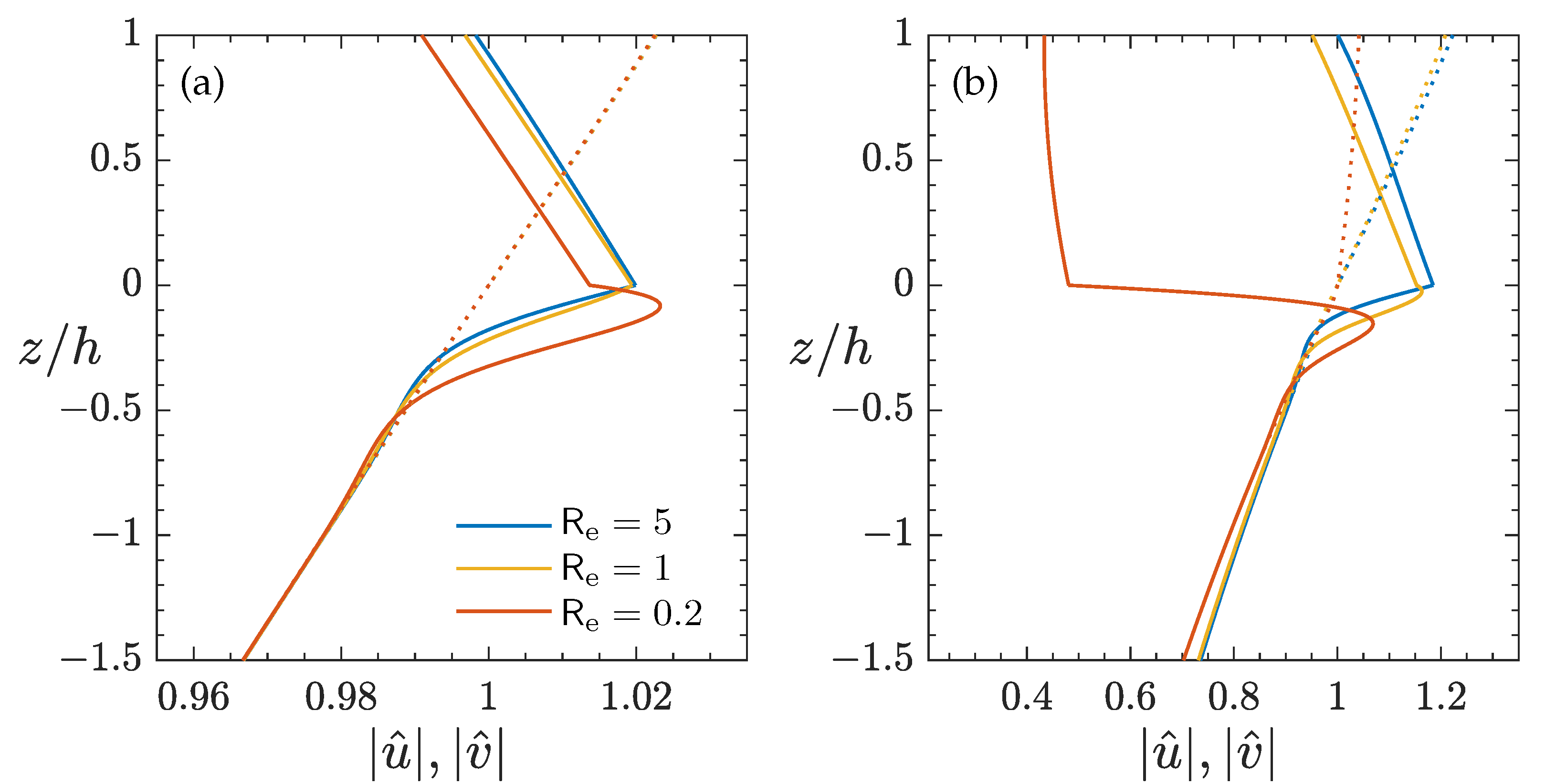
Examples are given in Figure 7 and Figure 8 showing the vertical profiles of $|\widehat{u}\left(z\right)|$ and $|\widehat{v}\left(z\right)|$. Recall that the velocity amplitudes $\widehat{u}\left(z\right)$ and $\widehat{v}\left(z\right)$ are complex functions in z, containing the phase relation between u and v. Here, we have scaled the velocities such that $|\widehat{v}(z=0)|=1$. This implies a normalization of $(u,v)$ using $a\omega$, where a is the characteristic wave amplitude of ${\eta }_2$, in view of Equation (9). In Figure 7, we examine the effect of the eddy viscosity of water, by fixing the ice-layer condition ${\mathsf{R}}_{\mathsf{e}}$ while varying the ice-to-water viscosity ratio ${\mathrm{\Pi }}_1$. The case of inviscid water (${\mathrm{\Pi }}_1=\infty$ for ${\nu }_2=0$) is included for comparison. In that case, $\widehat{u}$ is discontinuous at $z=0$ since the water is free to slip, and for $z<0$, the solution follows that of an irrotational deep-water wave; i.e., $|{\widehat{u}}_2|=|{\widehat{v}}_2|\sim {\mathrm{e}}^{k_{r}z}$ (see the results with ${\mathrm{\Pi }}_1=\infty$ in Figure 7). We then show the effect of ice-layer viscosity in Figure 8 by varying ${\mathsf{R}}_{\mathsf{e}}$, but holding ${\mathsf{R}}_{\mathsf{e}}{\mathrm{\Pi }}_1$ constant to represent the situation of fixing ${\nu }_2$.

In the viscous ice layer, the horizontal velocity amplitude $|{\widehat{u}}_1|$ increases downward towards the interface, in contrast to that of an irrotational linear wave, where $|\widehat{u}|$ decreases with depth. Since the water is less viscous than the upper ice layer, it can deform more freely under similar stress. Thus, at the interface, the water does not tend to resist the ice-layer flow. Instead, to compensate for its lower viscosity, the water velocity must develop an appreciably larger gradient $\partial u_2/\partial z$ in order to match the shear stress exerted by the ice flow at $z=0^{+}$, as required by the conditions of continuity across the interface. Immediately away from $z=0^{-}$ downward, $|{\widehat{u}}_2|$ decreases much more rapidly than ${\mathrm{e}}^{k_{r}z}$, signifying the WBL in water. At the outer edge of the WBL and beyond, $|\widehat{u}|\sim {\mathrm{e}}^{k_{r}z}$, as expected for the potential flow of the irrotational deep-water wave. The outer edge of the WBL is characterized by an ‘overshoot’, where $|{\widehat{u}}_2|$ briefly decreases beyond the potential flow solution before regaining and finally following it. Overshooting the targeted potential flow solution when approaching it is a typical feature of an oscillatory boundary layer. This vertical structure of $|\widehat{u}\left(z\right)|$ remains qualitatively similar as we vary the frequency, although for long waves, the changes in the velocity field are small over the thin depths in the ice layer and WBL.

For a greater eddy viscosity in water (i.e., smaller ${\mathrm{\Pi }}_1$), which may represent the strong mixing in a turbulent WBL due to intensified eddy activities, the velocity shear $\mathrm{d}|{\widehat{u}}_2|/\mathrm{d}z$ becomes weaker as the boundary layer thickens, with its outer edge intruding into the deeper depth. This reduces $|\widehat{u}(z=0)|$ at the interface and, consequently, affects the profile $|{\widehat{u}}_1\left(z\right)|$ in the ice layer. Specifically, for a relatively high $\tilde{\omega }$, the reduction of $|\widehat{u}(z=0)|$ only affects the lower part of the ice layer, decreasing the shear $\mathrm{d}|{\widehat{u}}_1|/\mathrm{d}z$ in the depths close to the interface, whereas near the upper surface, $|{\widehat{u}}_1|$ is little affected. For a low $\tilde{\omega }$, the reduction of $|\widehat{u}(z=0)|$ causes a decrease of $|{\widehat{u}}_1|$ in the entire ice layer because the long-wave oscillation can penetrate a shallow layer/depth relative to the wavelength without changing.

The vertical velocity amplitude $|\widehat{v}\left(z\right)|$ is little affected by the ice-layer viscosity or the presence of WBL in water, and closely follows the solution for an irrotational deep-water wave (i.e., $\widehat{v}\sim {\mathrm{e}}^{k_{r}z}$), except for a slight departure occurring in the ice layer when the wave is short (e.g., $\tilde{\omega }=0.6$); see Figure 7b,d. This is because v directly responds to the oscillations of the upper surface and interface, and, therefore, to the dynamic pressure determined by the irrotational component of the linear wave motion; see Equations (5), (9), (14c) and (16c).

For moderately low values of ${\mathsf{R}}_{\mathsf{e}}$, varying ${\nu }_1$ while fixing ${\nu }_2$ has only mild effects on $|\overline{u}\left(z\right)|$ and virtually none on $|\overline{v}\left(z\right)|$, regardless of the frequency; see the results with ${\mathsf{R}}_{\mathsf{e}}=5$ and 1 in Figure 8. For a highly viscous and thin ice layer, e.g., ${\mathsf{R}}_{\mathsf{e}}=0.2$, the velocity profiles are noticeably different from those with ${\mathsf{R}}_{\mathsf{e}}>1$. (i) In the ice layer, $|{\widehat{u}}_1\left(z\right)|$ is considerably reduced, in particular for high $\tilde{\omega }$. However, most interesting is the shear $\mathrm{d}|{\widehat{u}}_1|/\mathrm{d}z$. For a relatively low frequency wave, $\mathrm{d}|{\widehat{u}}_1|/\mathrm{d}z<0$ remains similar to that with ${\mathsf{R}}_{\mathsf{e}}>1$; but for sufficiently high $\tilde{\omega }$, a zero shear, $\mathrm{d}|{\widehat{u}}_1|/\mathrm{d}z=0$, tends to occur at an intermediate depth inside the ice layer, with a positive shear rate in the upper region close to the free surface. Such a profile of $|{\widehat{u}}_1\left(z\right)|$ becomes much more pronounced for $\tilde{\omega }>0.5$ with ${\mathsf{R}}_{\mathsf{e}}=0.2$. (ii) In contrast to the cases with ${\mathsf{R}}_{\mathsf{e}}>1$, where the water velocity $|{\widehat{u}}_2|$ continuously decreases inside the WBL, with ${\mathsf{R}}_{\mathsf{e}}=0.2$, $|{\widehat{u}}_2|$ first increases as we move away from $z=0^{-}$, reaches a maximum, and then begins to decrease towards the potential flow solution at the outer edge of the WBL; see the results with ${\mathsf{R}}_{\mathsf{e}}=0.2$ in Figure 8. For a high frequency (e.g., $\tilde{\omega }=0.45$ with ${\mathsf{R}}_{\mathsf{e}}=0.2$), the thin WBL is mostly characterized by an increasing $|{\widehat{u}}_2|$ because of the small interfacial velocity $|\widehat{u}(z=0)|$. The water velocity gradient $\mathrm{d}|{\widehat{u}}_2|/\mathrm{d}z$ in the vicinity of $z=0^{-}$ is determined by the stress condition (10). For a very low ${\mathsf{R}}_{\mathsf{e}}$ (i.e., highly viscous and thin ice layer), ${\nu }_1\partial v_1/\partial x$ (negative) can be great due to the large attenuation rate $k_i$, and dominates the total shear stress in the ice-layer flow, as ${\widehat{u}}_1$ and $\mathrm{d}|{\widehat{u}}_1|/\mathrm{d}z$ both become weak. Thus, to satisfy the stress conditions at $z=0$, the requirement for the water velocity gradient $\mathrm{d}|{\widehat{u}}_2|/\mathrm{d}z$ can be different from that with ${\mathsf{R}}_{\mathsf{e}}>1$. (iii) Despite the high ice-layer viscosity, the vertical velocity $|{\widehat{v}}_1\left(z\right)|$ for a low frequency wave still closely follows the variation $\sim {\mathrm{e}}^{k_{r}z}$ and becomes more uniform in z for high frequencies. Weber [5] argued that as the asymptotic limit of the ice layer is so thin and viscous, the horizontal motion is mostly suppressed and the ice layer oscillates more or less freely in the vertical direction, thus behaving like an inextensible surface film. Indeed, the solution of $|{\widehat{u}}_1|$ and $|{\widehat{v}}_1|$ with ${\mathsf{R}}_{\mathsf{e}}=0.2$ in Figure 8b indicates that the two-layer fluid system approaches such a limit as ${\mathsf{R}}_{\mathsf{e}}\to 0$.

The depth of the outer edge, $z=-r{\delta }_2$ where r is a constant may be used to estimate the WBL thickness. For example, with an ice-layer condition ${\mathsf{R}}_{\mathsf{e}}=5$, corresponding to the viscosity ratio ${\mathrm{\Pi }}_1=1000$, 100, 10, ${\delta }_2/h=\sqrt{2/\left({\mathsf{R}}_{\mathsf{e}}{\mathrm{\Pi }}_1\tilde{\omega }\right)}=$ 0.0258, 0.0816, 0.2582 for $\tilde{\omega }=0.6$. From Figure 7a, we read $r{\delta }_2/h\simeq 0.12$, 0.40,1.4 for the corresponding ${\mathrm{\Pi }}_1$ and therefore estimate $r\sim$ 4 to 6. For a low-frequency long wave $\tilde{\omega }=0.08$ in Figure 7b, ${\delta }_2/h$ is greater, and so is the WBL thickness, but the estimate of r is similar. As in the example given in Section 3.1, if $h=0.1$ m and ${\nu }_1=0.02$ m${}^2$/s for ${\mathsf{R}}_{\mathsf{e}}=5$, the WBL thickness for a wave of 1.1 s can be ∼0.14 m with an eddy viscosity ${\nu }_2=0.002$ m${}^2$/s in water.

3.4. Wave-Induced Reynolds Stress and Implication on the Steady Streaming

The time average of the product of linear flow velocities, $\overline{uv}$, is the wave-induced Reynolds stress, representing the mean momentum flux due to wave fluctuations [16]. For irrotational linear waves, $\overline{uv}=0$ identically; i.e., u and v are not correlated since v leads u by 90${}^{\circ }$. When the wave motion becomes rotational under the effects of viscosity, the phase relation between u and v is shifted and, consequently, $\overline{uv}\ne 0$.

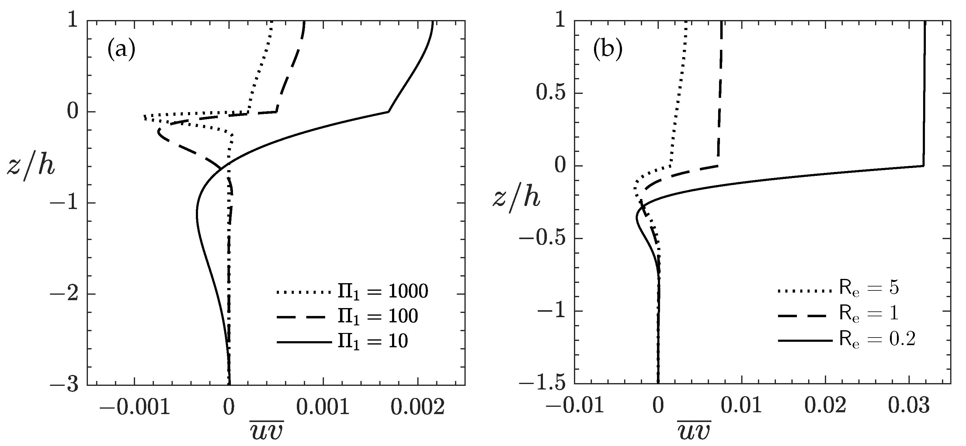
In the ice layer, $v_1$ leads $u_1$ by less than ${90}^{\circ }$. As a result, $\overline{uv}>0$ for $0<z/h<1$ and decreases mildly from the upper surface to the interface (Figure 9). Inside the WBL and as we move away from $z=0^{-}$, $\overline{uv}$ first decreases rapidly, reaches a negative peak (${\overline{uv}}_{min}<0$), and then returns to approach $\overline{uv}=0$ at the outer edge $z\sim -r{\delta }_2$ and beyond in the inviscid core. This vertical structure of $\overline{uv}$ is generally observed as we vary ${\mathsf{R}}_{\mathsf{e}}$ and ${\mathrm{\Pi }}_1$, as well as $\tilde{\omega }$, despite the differences in the magnitude of $\overline{uv}$ and in the thickness of WBL. Increasingly, either ${\nu }_1$ or ${\nu }_2$ will increase $\overline{uv}$ for $0<z/h<1$ in the ice layer. This is consistent with the fact that a major effect of viscosity is to induce a phase shift between the two waves and affect the phase relation between u and v.

The Reynolds stress $\overline{uv}$ is a nonlinear quantity obtained from the linear wave theory, therefore being of the second order in wave slope $O\left(a{k}_r\right)$. However, it is physically significant, since it is a driving force for the wave-induced mean flow. For waves on an open-water surface, it is well understood that a steady flow must exist in order to provide a mean shear stress to balance the wave-induced Reynolds stresses due to the viscous effects of wave boundary layers at the surface and seabed [16]. This mean flow is called Eulerian steady streaming, and when combined with the Stokes drift, gives the fluid particle (Lagrangian) drift, i.e., the mass transport in water waves following [15].

While $\overline{uv}$ is a main driving force, determining the mean flow field necessitates a formal nonlinear analysis to account for other processes, including the mean dynamic pressure and momentum fluxes due to wave attenuation, nonlinear effects of surface, and interface curvatures in the boundary and interface conditions, as well as the lateral boundary conditions in the wave propagation direction (e.g., whether the system is closed or open). Such a nonlinear analysis may be formulated using a method analogous to studies of mass transport in water waves over a mud layer (e.g., [35,36]). That is beyond the scope of this study, but we may nevertheless make a very preliminary speculation on steady streaming based on $\overline{uv}$.

When the wave amplitude is small relative to the thickness of the wave boundary layer, the vorticity dynamics are dominated by viscous diffusion [15]. Assuming $\partial /\partial x\equiv 0$, i.e., a uniform condition in the wave propagation direction and negligible wave attenuation, the equation for the streaming velocity $\overline{u}$ may be written as [16]

$$\nu \frac{{\partial }^2\overline{u}}{\partial z^2}=\frac{\partial \overline{uv}}{\partial z}.$$

(25)

Suppose Equation (25) can be applied in the thin ice layer, and in the WBL at the interface. We integrate it separately for $0<z<h$ and $z<0$ using the appropriate viscosity. Assuming that (i) the mean stress vanishes outside the WBL, i.e., ${\nu }_2\partial {\overline{u}}_2/\partial z\to 0$ for $z\ll -r{\delta }_2$; that (ii) the continuity of mean stress at the interface can be approximated as

$${\rho }_1{\nu }_1\frac{\partial {\overline{u}}_1}{\partial z}={\rho }_2{\nu }_2\frac{\partial {\overline{u}}_2}{\partial z}\mathrm{at}z=0;$$

(26)

and that (iii) the mean velocity is continuous at $z=0$, i.e., ${\overline{u}}_1\left(0\right)={\overline{u}}_2\left(0\right)=\overline{u}\left(0\right)$, we obtain

$$\begin{array}{ccc}\hfill {\overline{u}}_1-\overline{u}\left(0\right)& =\hfill & \hfill {\nu }_1^{-1}\left[{\int }_0^z\overline{uv}\mathrm{d}z+({\mathrm{\Pi }}_0^{-1}-1)\overline{uv}{|}_{z=0}z\right]\mathrm{for}0<z<h,\end{array}$$

(27a)

$$\begin{array}{ccc}\hfill {\overline{u}}_2-\overline{u}\left(0\right)& =\hfill & \hfill {\nu }_1^{-1}{\mathrm{\Pi }}_1{\int }_0^z\overline{uv}\mathrm{d}z\mathrm{for}-r{\delta }_2<z<0.\end{array}$$

(27b)

Mathematical details are given in Appendix A. Equation (27b) is only valid inside the WBL. At the outer edge $z\sim -r{\delta }_2$, it provides a condition for determining the mean flow field in the inviscid region $z\ll -r{\delta }_2$. The mean velocity $\overline{u}\left(0\right)$ at the interface can be determined with additional information, e.g., conditions at the upper surface, matching at the outer edge of the WBL with the inviscid region (once the nonlinear analysis is carried out), or constraints on the depth-integrated transport depending on the lateral boundary conditions.

To explore the effects of ${\mathsf{R}}_{\mathsf{e}}$ and ${\mathrm{\Pi }}_1$, we can recast Equation (27) into the dimensionless form by normalizing $u,v$ using $a\omega$ (or equivalently, $|\widehat{v}(z=0)|$) as in Section 3.3. Sample calculations are given in Figure 10 for a low frequency $\tilde{\omega }=0.08$ such that the attenuation rate ${\tilde{k}}_i$ is small and the wave propagation is approximately uniform in x. The factor $a/h$ is excluded from the calculations (see Appendix A). The calculations are for waves propagating in the $+x$ direction. A few points are worth noting. (i) Relative to the interfacial mean velocity $\overline{u}\left(0\right)$, the streaming current in the WBL under the ice is much more pronounced, clearly indicating that the phenomenon is related to the boundary layer flow because of the high shear rate. (ii) Relative to $\overline{u}\left(0\right)$, the streaming current in the ice layer is forward in the direction of wave propagation, while immediately beneath the ice, it tends to be backward in the WBL. (iii) For a smaller viscosity ratio, which may represent a turbulent WBL with a large ${\nu }_2$ due to strong mixing, the backward relative streaming velocity occurs throughout the WBL, and ${\overline{u}}_2-\overline{u}\left(0\right)\to 0$ at the outer edge $z\sim -r{\delta }_2$; in the ice layer, the forward velocity ${\overline{u}}_1-\overline{u}\left(0\right)$ becomes stronger (see the curve for ${\mathsf{R}}_{\mathsf{e}}=5$ and ${\mathrm{\Pi }}_1=10$ in Figure 10). On the other hand, with a greater viscosity contrast, ${\overline{u}}_2-\overline{u}\left(0\right)$ reverses direction and becomes forward inside the WBL. The larger the viscosity ratio is (e.g., due to increasing ${\nu }_1$ while keeping ${\nu }_2$), the stronger the backward relative streaming velocity becomes under $z=0^{-}$, but a weaker forward ${\overline{u}}_2-\overline{u}\left(0\right)$ is reached at the outer edge; see the results with ${\mathsf{R}}_{\mathsf{e}}=5$, ${\mathrm{\Pi }}_1=100$, and with ${\mathsf{R}}_{\mathsf{e}}=1$, ${\mathrm{\Pi }}_1=500$ in Figure 10. Furthermore, ${\overline{u}}_1-\overline{u}\left(0\right)\simeq 0$, indicating that in an average sense, the water feels the ice layer as if it were a deformable ’solid plate’ rather than a fluid layer because of the great contrast in their viscosities. (iv) A large mean shear $\mathrm{d}{\overline{u}}_2/\mathrm{d}z$ in the WBL is theoretically expected for a large ${\mathrm{\Pi }}_1$ because of the stress condition at the interface, but may be unattainable in real fluids since shear instability would most likely occur. The subsequent, enhanced mixing would certainly alter the streaming velocity profile, likely towards one similar to that with a smaller ${\mathrm{\Pi }}_1$. (v) At the outer edge of the WBL, ${\overline{u}}_2$ tends to be uniform and remains so just outside, in the region where the depth is greater than $r{\delta }_2$, but it is still small compared with the wavelength. This allows matching with the mean flow in the inviscid core where the length scale of the flow is characterized by the wavelength. For a complete determination of the profile ${\overline{u}}_2\left(z\right)$ outside the WBL, one needs to carry out nonlinear analysis for the inviscid core.

While these are speculations based on crude assumptions and will likely be revised by a rigorous analysis, there seems to be some relevance. Processing their PIV data using proper orthogonal decomposition, Rabault et al. [14] showed the existence of a mean water flow under the grease-ice layer in the opposite direction of wave propagation. In an earlier study, Martin and Kauffman [37] also indicated a backward flow at the ice–water interface when illustrating the mean circulation in grease ice with an increasing thickness towards the beach-end of the wave tank. Rabault et al. argued that the back-flow may be due to the packing of ice, which, as a consequence of mass conservation, causes a counter-current of water in the opposite direction. However, on the other hand, ice piling up in itself can be an indication of a forward drifting current in the upper layer, relative to the water. From the discussion above in (iv), a mean flow profile with a smaller viscosity ratio is likely to be observed, in view of the shear-induced mixing. Taking, for example, the case with ${\mathsf{R}}_{\mathsf{e}}=5$ and ${\mathrm{\Pi }}_1=10$ in Figure 10, we may argue that $\overline{u}(z=0)$ is nearly zero or at least very small, since in the case of deep water depth, we expect ${\overline{u}}_2\to 0$ for $z\ll -r{\delta }_2$, and it already happens that ${\overline{u}}_2-\overline{u}\left(0\right)\sim 0$ at $z\sim -r{\delta }_2$. Thus, we see that under the combined effects of ice and water viscosities, the wave-induced Reynolds stress can drive a forward streaming in the upper ice layer and a backward, relatively strong streaming in the water just underneath the ice.

4. Summary and Concluding Remarks

We have re-considered the problem of linear waves on ice-covered seawater, with a particular interest in the effects of the wave boundary layer (WBL) in the water just underneath the ice. The thin, viscous upper layer is a mathematical representation of the soupy ice-agglomeration in marginal ice zones, and is treated as a Newtonian incompressible fluid. The seawater viscosity is only important in the WBL because of the high shear rate in the velocity field there. Outside the WBL, the wave motion is essentially inviscid and the water depth is deep. While existing studies tend to focus on the dispersion relation, in particular, the wave attenuation by ice, we have paid special attention to the velocity distributions in the ice-layer flow and the boundary water flow, the Reynolds stress induced by the linear wave fluctuations, and its implication on Eulerian steady streaming. Key results are summarized, as follows.

(i)

The presence of a WBL under the ice layer can significantly affect the theoretical result of the wave attenuation rate at low frequencies, and therefore has a stronger implication in large-scale applications. With a reasonable value of water eddy viscosity, the theoretical solution agrees very well with the observed attenuation rates over a large range of frequencies covering both field and lab waves, significantly outperforming the previous result assuming an inviscid water. It also offers a possible physical basis for the recently proposed empirical formula of wave attenuation that explicitly incorporates dependence on ice thickness, but is obtained from data-fitting [13].

(ii)

Under the ice, the WBL in water is enhanced and can have a thickness comparable to the ice-layer thickness, even for short waves of high frequencies. Varying either the effective ice-layer viscosity or water eddy viscosity can alter the fluid velocity profiles in both the ice layer and WBL, because of the continuity of stresses and velocities across the interface. While the WBL is thicker for low frequencies and therefore causes a greater total dissipation, the shear rate is much stronger in the thinner boundary layer of a high frequency wave and can be subject to instabilities. When the ice layer is so thin and so viscous that the time scale of vorticity diffusion in the ice flow is faster than the inertial time scale of wave motion, the horizontal ice-flow velocity is greatly restricted at sufficiently high frequencies, and asymptotically, the ice layer behaves as an inextensible thin surface film; the water velocity in the WBL exhibits a more complex vertical structure.

(iii)

The effects of viscosities modify the phase relation between the horizontal and vertical velocity of the linear flow, such that a Reynolds stress distribution is established in the ice layer and WBL. This mean momentum flux due to wave fluctuations drives the secondary induced mean flow. Speculation based on crude assumptions indicates that, relative to the ice–water interface, the steady streaming in the upper ice layer is forward in the direction of wave propagation, while in the WBL just underneath the ice, a backward streaming current tends to occur.

While we have briefly remarked on the qualitative similarity between some features of the theoretical flow field and observations, an in-depth comparison needs to be conducted, for example, using the PIV measurements from the large-scale wave tank experiments at the U.S. Army Corps of Engineers Cold Regions Research and Engineering Laboratory (CRREL), which is an ongoing NRL study [38].

Since linear solutions are often applied in practical problems and are the first step in nonlinear analyses, the results of this study will contribute to the literature and guide applications. The analysis in this study is for monochromatic waves, but can be extended to random waves. Still, the results here can shed some lights on spectral waves interacting with sea ice. For instance, the ice thickness is expected to be thin near the ice edge, where high frequency waves likely survive and contribute considerably to the total wave energy, whereas low frequency waves can penetrate far into ice fields of greater thickness and likely dominate the wave energy spectrum there. Thus, the behavior of the theoretical solution, according to the dimensionless frequency normalized using the ice thickness, can inform wave–ice interactions in those different regions.

For the nonlinear analysis aiming at the Lagrangian mass transport in the two layers of fluids, one can in principle follow the approaches in the literature, e.g., using the Lagrangian description of the flow equations for both fluids (e.g., [35]) or an orthogonal curvilinear coordinate system (e.g., [36]). This will relax the constraint on the wave amplitude, which is a strong limitation when applying a linear wave theory. In such a nonlinear analysis, the effects of surface and interface curvatures will be properly accounted for and can be significant, given the important role played by the interface conditions in facilitating wave–ice interactions, as we have seen in this study. Wave attenuation is another cause of mean momentum flux and can strongly influence the mean flow field in regions where high frequency waves are active.