Assessment of the Black Sea High-Altitude Wind Energy

Abstract

Airborne wind energy systems (AWESs) represent a novel idea that aims to gather energy from stronger winds aloft while operating at altitudes above conventional wind turbines (WTs). For this study, we examined the wind resources at a height of 100 m available for traditional wind turbines with aerial wind energy technologies, in addition to the wind potential at higher altitudes up to 500 m. The considered period was 20 years from January 2002 to December 2020, and the data were extracted from the ERA5 reanalysis database. We studied the possibility of placing 500 kW and 5 MW airborne systems in the Black Sea and the Azov Sea and compared them with a conventional turbine. As expected, the western part of the Black Sea presented the best results, both for the 500 kW airborne system with an annual energy production (AEP) of 2.39 GWh and a capacity factor of 55%, and for the 5 MW airborne system, which has an annual electricity production of 15.81 GWh and a capacity factor of 36%. Better results were recorded for the Sea of Azov for both the 500 kW and the 5 MW airborne systems, with an AEP of 2.5 and 15.81 GWh and a capacity factor of 58% and 36%, respectively.

1. Introduction

Perhaps the oldest form of non-conventional energy used by man was wind energy, scientifically called aeolian energy [1]. This is produced using the kinetic energy of the wind, obtained through a self-generating device. Wind power depends on weather conditions, making it an intermittent source of electricity. The air density varies in some parts of the Earth due to differences in heating. These variations cause the movements of large air masses. The first windmills appeared in the 15th century after people had noticed how quickly the air moves. By using wooden and canvas paddles, the movement of air masses was converted into a rotational action.

The development of wind energy is driven by three important challenges: energy security, climate change, and the need to reduce greenhouse gas emissions, in addition to access to energy [2]. The global expansion of wind energy continued in 2021, registering a growth three times higher than that of 2020 despite the pandemic. The total global installed capacity of wind energy reached approximately 850 GW in 2021 [3], of which offshore wind energy was approximately 55 GW [4]. The year of 2021 was the first in which renewable energy exceeded energy from coal. Green energy generated approximately 38% [5] of the world’s global energy, in the pandemic context and due to the desire to reduce CO₂ emissions following the Paris Agreement [6]. Recently, one of the most exploited energy sources has been wind energy. Although onshore wind energy was predominantly exploited initially, as a result of the decrease in the amount of fossil fuels, offshore wind energy has become one of the most exploited energy sources in recent times. The main reason for this is that offshore wind energy is more abundant and much more advanced technologies can be used to generate electricity. Due to technological advances, increasingly larger turbines have started to be used in the field of offshore wind energy. The first offshore wind turbine used was a 450 kW turbine produced by Bonus Energy, which later became Siemens Gamesa. This turbine was used as part of the first Vindeby offshore wind farm in 1991, built by Denmark. At higher altitudes above the ground, the wind can move more freely and with less resistance, which is typically provided by structures on the Earth’s surface such as trees, buildings, and mountains. As a result, wind speed generally increases with altitude. For instance, the largest offshore site ever built (Hornsea Project One, UK) measured an average wind speed of 9.6 m/s at a height of 100 m (tower hub height) [7], and 10.6 m/s at a height of 200 m. In order to take advantage of the stronger high-altitude winds, the current main tendency is to build taller wind turbines that are fitted with longer blades; for example, the Chinese MySE 16.0–242 [8,9], which will have a 16 MW maximum output, will have a diameter of 242 m. Another important factor is the average distance to shore, which has been steadily increasing over time [10,11]. The early projects had short average distances to the shore, but as time advanced, this distance increased quickly; projects in the range of 100 and 200 km were developed, according to the data available for 2020 [12]. Therefore, if the wind turbines are to operate under wind farm settings or in the areas of the Earth’s atmospheric boundary layer [13], where energetic, coherent turbulence is known to exist for a major portion of the turbine running time, they must be properly built.

There are at least three distinct vertical sections or layers that make up the planetary boundary layer (PBL) of the Earth’s atmosphere. For wind turbines, the surface and mixed layers are crucial. Wind flowing over flat, uniform terrain is considered to be in the surface layer, which is the place where wind turbines are located. The characteristics of turbulence in the surface layer include a nearly constant vertical momentum flux with height, a positive (upward) heat flux during the day, and a negative (downward) flux at night [14]. Because of friction, the vertical flow of turbulent kinetic energy (TKE) is positive, moving away from the surface. The convective surface layer during the day differs greatly from the nocturnal surface layer during the night. The turbulent eddies are relatively large during unstable daylight hours but, at night, under stable conditions, they tend to be considerably smaller and more coherent or structured because the negative buoyancy slows vertical motions. Under conditions of intense surface heating, this layer can frequently reach a depth of 100–150 m [14] or 10% of the overall boundary-layer depth. Depending on the wind speed, the nighttime or stable surface layer is typically significantly thinner, varying from 10 to 50 m [15].

At higher altitudes, the wind is often stronger and more persistent in most parts of the world. Airborne wind energy (AWE) [16,17] systems are intended to harness this energy potential, which is inaccessible to conventional ground-based wind turbines. The idea of harvesting wind energy using aerial wind turbines (AWTs) is new and exciting. This concept involves transforming the CWT’s blades into a power kite that flies quickly and perpendicular to the wind. The kite’s top is equipped with a turbine, an electrical generator, and a power electronic converter. The generated electricity is sent to the ground via a medium-voltage cable [18]. According to Betz’s Law, only a tiny swept area of the turbine and/or a turbine of low weight are needed for the generation of a given amount of electric power because the power kite flies at a high speed that is several times faster than the actual wind speed. The size of the generator is further reduced since the high turbine rotational speed eliminates the requirement for a gear transmission. The power kite’s takeoff and landing turbines and generators serve as motors and propellers, respectively, by generating energy that enables the system to be operated similarly to a helicopter. Among the various AWES ideas, we can distinguish between Ground-Gen systems, which convert mechanical energy into electrical energy on the ground, and Fly-Gen systems, which do this on the aircraft [19]. The AWES concept is a highly attractive one, taking into account that 30% of the length of a blade produces more than half the power of a conventional turbine [20,21].

Since the airborne wind energy sector is still in the early stages of development, there are few studies focused on these topics, and very little information regarding the Black Sea potential. In the work of Bechtle et al. [22], the ERA5 wind dataset was used to provide a spatial analysis of the wind resources from Europe. Nevertheless, in this case the target area stretches between the western part of Portugal and the eastern part of the Mediterranean Sea, and no additional info was provided outside this region. Although the authors also took into account the wind resources at the 800 m level, based on various trials it was found that the average operational height for a pumping kite is in the range of 150–500 m. Moreover, this work focused only on the resource assessment, without taking into account the performance of a particular AWES, which was the aim of the present work. In the work of Li et al. [23], the high-altitude wind resources of China were also investigated using the ERA5 dataset, which was adjusted for a 300 m altitude. Several sites were taken into account from the coastal areas of Bohai, Nanhai, and Donghai Sea in order to identify the most promising in terms of wind energy resources. Based on these results, it was found that the U300 conditions (average) can easily reach values in the range of 6.89 to 11.58 m/s. In the work of Lunney et al. [24], the high-altitude wind resources from Northern Ireland were taken into account, which were considered feasible to develop these type of projects up to 3000 m above the ground level. In addition to the resource assessment, it was estimated that the initial budget for a pilot project of 2 MW would be close to GBP 1,751,402 per unit, which was associated with a LCOE value of 0.106 GBP/kWh. It should also be mentioned that a significant part of the existing literature is dedicated to development of the AWES models, and is divided between designing studies [25], optimization [26], or layout configuration [27].

In this context, the aim of this work was to provide a general overview of the Black Sea wind resources by making a direct comparison between the conditions reported at 100 m, where most of the offshore wind turbines operate, and those reported at much higher levels (e.g., 400 m) where AWES generators may be found in the future. In addition to the resource assessment, the performance of various wind converters was considered for evaluation. To the best of the knowledge of the authors, this is one of the first studies to discuss the use of Black Sea high-altitude wind energy, which can be considered to be an element of novelty.

2. Materials and Methods

2.1. The Black Sea

The Black Sea is characterized by an area of 423,000 km² and a water volume of 547,000 km³, and has a maximum depth of 2200 m. In the north-western area there is a continental shelf that covers around 25% of the total basin; in this region, depths are greater than 160 m. In the western area the most important rivers are located (Danube, Dniepr, and Don), of which the Danube makes a significant contribution with almost 209 km³ of water discharged per year, followed by the Dniepr, at 44 km³/year. The Black Sea is considered to be the largest anoxic water body on our planet, due to the fact that only 10% of the water volume is associated with the presence of oxygen. Although it is considered to be an enclosed basin, there are some outlets that allow maritime exchanges with the neighboring areas, namely the Bosphorus Strait (<75 m depth) and the Kerch Strait (≈8 m depth) [28]. The Black Sea climate can be described as continental, while the air circulation is a complex one, being influenced by seasonal and regional features. During winter, the influence of the dry and cold winds from the north-west is visible, which significantly reduces the water temperature and generates severe storms. For example, during the extreme wind Bora (Novorossiysk) the local harbors can be shut down for 70 days/year when the wind speed can increase to 30 m/s. In contrast, the eastern and south-eastern regions are shielded by the Caucasus Mountains and, therefore, warmer conditions are noticed. In the summer, the weather is generally stable with clear skies, and the regional weather pattern is controlled by the Azores high-pressure conditions that generate an anticyclonic air distribution over the Black Sea [29].

2.2. The Wind Data

Currently, the ERA5 dataset is considered to be one of the most reliable sources of information for land and ocean variables, and is, in fact, an improved version of the ERA-Interim project that was stopped at the end of 2019. The idea behind this project is to use an advanced modeling system that incorporates various sources of observations (in situ and satellite) through a data assimilation approach [30]. The satellite missions produce scatterometer data from satellites such as ERS-1, OCEANSAT-2, and QUIKSCAT, while the altimeter section is represented by missions such as JASON-2, CRYOSAT-2, and SARAL. In terms of in situ measurements, the measurements related to the marine environment are related to drifting and moored buoys, radiosondes, and aircraft data. The ERA5 model is based on a 4D-Var model that involves 12 h assimilation windows (9-21 UTC/21-9 UTC), and therefore the quality of the observations during the time interval will influence the accuracy of the model. Furthermore, the variables produced in this way are related to average values influenced by the grid box and time step of a particular model, so significant differences may occur when comparing data for particular in situ locations [31].

The ERA5 wind data were processed for a 20-year interval (January 2002–December 2021), considering the entire Black Sea region and the wind conditions related to a 100 m height (U100), and were directly obtained from the Copernicus data store. The U100 parameter is frequently used for marine sites, either to assess the wind energy potential [32] or to estimate the performance of an offshore turbine that can be easily adjusted to this height [33]. In contrast, the philosophy behind the AWES systems is to operate at much greater heights (e.g., 1000 m), as in the case of the Kite Gen project [34]. The wind speed is significantly higher as height increases to the atmospheric boundary layer, with this dependency following a logarithmic law [35]. Therefore, it is necessary to adjust the initial dataset to a particular Airborne Wind Energy System (AWES) operational height, and this can be done using the logarithmic wind profile as follows [36]:

$$U_{AWES}=U_{ERA5}\frac{\ln \left(z_{AWES}\right)-\ln \left(z_{ERA5}\right)}{\ln \left(z_{ERA5}\right)-\ln \left(z_0\right)}$$

(1)

where U_AWES—wind speed adjusted for a particular AWES; U_ERA5—wind speed associated with ERA5 data (U100 in this case); Z_AWES—operating height of an AWES; Z_ERA5—ERA5 wind data reference height (100 m in this case); z₀—roughness length of the sea surface (0.2 mm) [37]. It is important to mention that although this method seems to be less accurate for higher atmospheric layers, it is reliable enough to estimate the marine wind resources according to the information provided in Schelbergen et al. [38].

The ERA5 project provides wind data at 10 (U10) and 100 m (U100) levels. For the present work, only the U100 parameter was considered for four-hourly intervals (corresponding to 00:00:00, 06:00:00, 12:00:00, 18:00:00) of each day in order to avoid possible uncertainties that may occur when using the wind logarithmic law. For example, in the work of Sapian [39], the profile of the wind speed significantly increases in the range of 10–100 m, being followed by a more constant evolution at higher altitudes, especially in the case of the marine areas [40].

2.3. Wind Generators

The performance of a particular wind turbine (three-blade system) can be expressed through a power curve, which makes a direct connection between the expected power and a particular wind speed. Compared to a classical wind turbine, the performance of a particular AWE system is influenced by numerous factors, such as flight altitude, wind area, and the aerodynamic coefficients (lift and drag) [21]. In order to make a direct comparison between different types of wind generators, some researchers also proposed a power curve for AWES generators, e.g., Weber et al. [35]. Figure 1 presents these curves, including a 5 MW wind turbine and two AWES systems (500 kW and 5 MW); these three systems will be further considered for evaluation. According to this information, the performance of the wind turbine will be evaluated for a hub height of 100 m, compared to the AWES, where two operating heights will be used (200 and 414 m). At this point, it is important to mention that, in Weber et al. [35], a clear distinction is made between an airborne system with rigid and flexible winds, whereas in the present work only the information related to the generic power curves is used.

The power curve shapes indicate a clear distinction between the wind turbines and the AWES. In the case of the turbine, at some point the system reaches maximum power production (5 MW in this case), which remains constant until a cut-out value of 25 m/s is reached, when the generator is shut down for safety reasons. Nevertheless, an airborne generator operates on a different principle; this is the case of the kite system considered in this work, which has a traction phase (energy is generated) and a retraction phase (energy consumed). In the pumping cycle, the kite moves away from the ground stations and reaches a maximum altitude related to the tether length; this is followed by a reel phase when the kite is pulled back to the ground and loses energy [41]. This aspect is reflected in the power curves of the two AWESs (5 MW and 500 kW), where there is a decrease in power after a maximum peak is reached.

Subsequently, the annual electricity production (or AEP) can be estimated as follows [42]:

$$AEP=8760\times {{\displaystyle \int }}_{cut-in}^{cut-out}f\left(u\right)P\left(u\right)du$$

(2)

where: 8760—number of hours in a year; cut-out/cut-in—wind turbine operational limits; f(u)—Weibull probability density function; P(u)—turbine power curve.

The capacity factor (Cf) is frequently used to measure the reliability of a particular energy system, and is defined in this case as the ratio between the expected power to be generated from a particular wind turbine (P_turbine) and the rated power of a generator (P_rated) [42]:

$$Cf=\frac{P_{turbine}}{P_{rated}}$$

(3)

3. Results

A first overview of the Black Sea wind resources is provided in Figure 2, which represents the spatial distribution of the U100 parameter (average values). As expected, the central and western parts of this region present more consistent values, with much higher values shown for the Azov Sea (located to the north). The maximum values reach 8–8.2 m/s and gradually decay toward the east, where a minimum of 2 m/s may be encountered near the coastal areas of Georgia and Türkiye. The Crimea Peninsula shows more important resources in the western part, whereas in the eastern area a hot spot defined by a value of 5 m/s is highlighted. For the western coastal area, the wind conditions in the range of 6 to 8 m/s represent a common occurrence, especially in the case of the Romanian nearshore.

Figure 3 presents the seasonal distribution of the U100 parameter, where: winter (December-January-February); spring (March-April-May); summer (June-July-August); autumn (September-October-November). In terms of the spatial distribution, a similar pattern is noticed; in the case of the full-time distribution (Figure 2), more important resources are concentrated in the center and western regions, regardless of the season taken into account. During winter, a maximum of 9.16 m/s is expected near the Azov Sea, compared to the value of 8.81 m/s that may occur on the western part of the Black Sea. In less energetic seasons, the values decrease for the Azov Sea to 7.88 m/s (spring), 6.61 m/s (summer), and 8.19 m/s (autumn); and for the Black Sea to 7.42, 6.33, and 7.53 m/s, respectively. The coastal areas located on the eastern side are defined in general by a wind speed of 3–4.5 m/s during winter and spring, including a hot spot (central part of Georgia) where a maximum of 6.5 m/s may occur. For the remaining seasons, the wind conditions from the west do not exceed 5 m/s, even in the case of the offshore areas. The Azov Sea is defined by wind conditions that frequently exceed 8 m/s, except during the summer when, close to the coastal areas, a minimum of 6 m/s may be noticed.

Figure 4 presents the differences between two different wind fields (U500 and U100) considering the entire datasets. The U500 parameter was considered for comparison, since this may represent an average height at which an airborne system may operate. The expected variations are in the range of 0.3 to 1 m/s, dividing this map into three distinct areas, namely: (a) the Azov Sea and western part of the Black Sea—0.8 and 1 m/s; (b) Black Sea, coastal areas from the west, north, and east (offshore)—0.55 and 0.8 m/s; and (c) Black Sea, coastal areas from the south and east—differences <0.5 m/s.

A similar analysis is provided in Figure 5, considering this time the seasonal distribution. As expected, the Azov Sea is defined by the maximum values indicating maximum differences of 0.9 and 1.2 m/s. During the winter, for the central part of the Black Sea, values of 1 m/s are seen, which can increase to 1.1 m/s in the offshore areas from the west. In the case of spring, most of the region is defined by differences that are higher than 0.8 m/s, except for the eastern side where the values decrease to 0.3 m/s. The summer season reveals multiple wind fields, and the differences gradually decrease from the western part of Crimea to the south-west, and from the north to the south-east (Georgia), where a minimum of 0.3 m/s is highlighted.

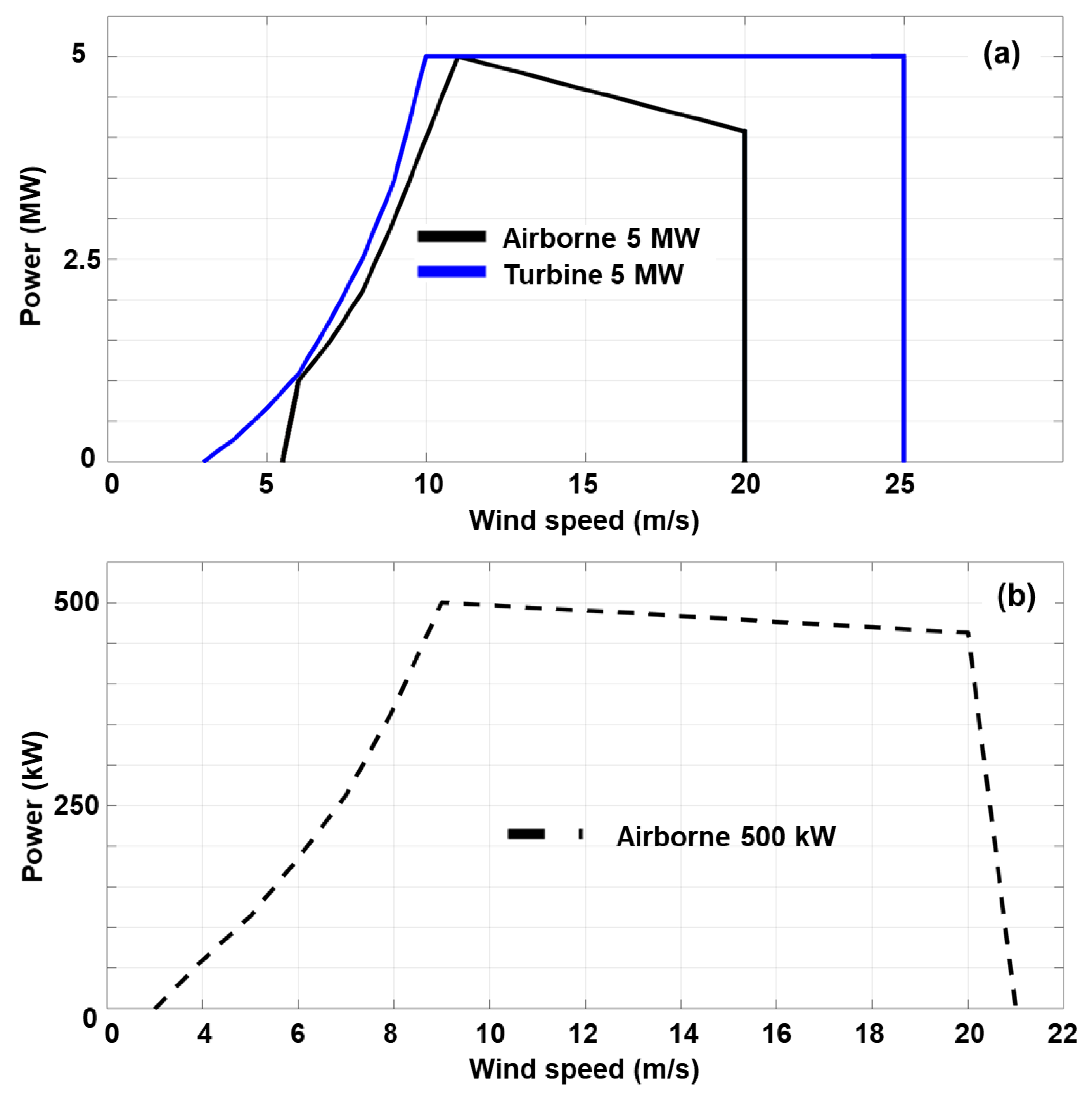
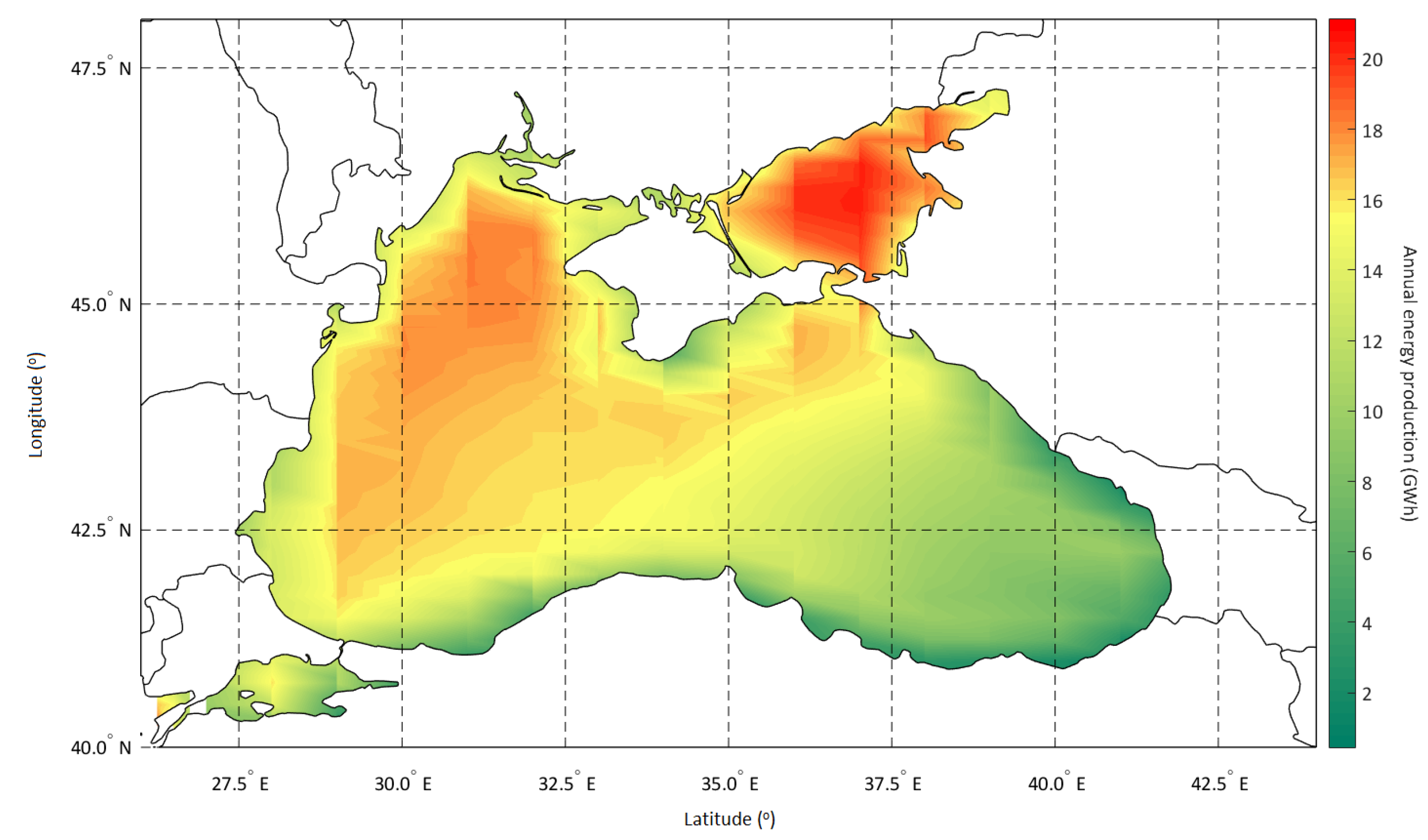
Figure 6 highlights the expected annual energy production (or AEP) of the 5 MW wind turbine (classical system), using the wind resources associated with a hub having a height of 100 m. The energy production is directly related to the wind energy potential and, as a consequence, much higher values are noticed near the Azov Sea (20.43 GWh), followed by the north-western sector where a maximum of 18.47 GWh may be generated. Near the coastal areas from the west and north, production in the range of 12 to 15 GWh may be expected, compared to the south-east where the values drop to a minimum of 2 GWh.

Following the performance of the 5 MW turbine, Figure 7 shows a spatial distribution of the capacity factor (in %). A maximum of 47% is expected close to the Azov Sea, whereas for the western sector of the Black Sea these values reach a maximum of 42%. Nevertheless, regarding the coastal areas where the offshore wind farm operates, more realistic values of 30%–35% may be expected for most of the Black Sea regions, except for the eastern part. For this sector, the values gradually decrease from 23% (offshore) to a minimum of 5% (near the coast), which indicates that this type of turbine is not recommended for such a coastal environment.

A first perspective of the AWES performance is provided in Figure 8, considering the annual electricity production of the 500 kW system, which has an average flight altitude of 200 m. The values gradually increase from 0.5 GWh (eastern coasts) to 1.25 GWh (eastern offshore), and finally reach maximum values of 2.39 GWh in the western sector. From the two EU countries (Romania and Bulgaria), minimum production of 1.5 GWh may be expected close to the coastline.

Figure 9 presents the capacity factor of the previously mentioned airborne system (500 kW). According to this indicator, the maximum values oscillate between 55% and 58%, with better performances being expected near the Azov Sea. The offshore region located between 30° and 32.5° from the Black Sea is defined by more consistent values, which decrease to a capacity factor of 35% toward the western coastlines. Regarding the eastern sector, the performance of this AWES is relatively close to the performance of the wind turbine (5 MW), reaching a minimum of 10%.

For higher-capacity production, Figure 10 presents the spatial distribution of the AEP indicator associated with an airborne system defined by a rated capacity of 5 MW, which is capable of operating at an altitude of 200 m. At this point, the performance is evaluated for two different flight altitudes, and the expected results are further used to make a direct comparison with the classical wind turbine (5 MW). For this operational height, the 5 MW AWES has much lower electricity production than the traditional wind turbine, with an expected maximum of 16.33 GWh near the Azov Sea. For the Black Sea, the values reach a maximum of 14.34 GWh in the north-western sector and gradually decrease to 10 GWh toward the south-west. The south-eastern area is defined by values of 8 GWh near the latitude line of 43°, and finally reach 2 GWh in the vicinity of the eastern shoreline.

Figure 11 illustrates the capacity factor of the 5 MW airborne system (U200), for which a maximum value of 37% for the Azov Sea can be highlighted. For the Black Sea area, this indicator is defined by values in the range of 5% to 33%, according to the region of interest, such as the offshore north-west and coastal areas from the east.

Figure 12 and Figure 13 present the performance of the 5 MW AWES at a reference height of 414 m, with the result indicated in terms of annual electricity production and capacity factor, respectively. A similar spatial pattern is observed as in the case of the U200, while the performance of the AWES increases to 17.66 GWh (Azov Sea), which is associated with a capacity factor of 40%. For the Black Sea, the best performance is related to the western sector, of 15.81 GWh for the AEP and a capacity factor of 36%.

4. Discussion

The Black Sea wind conditions are clearly of interest from a renewable and meteorological point of view. This aspect was better highlighted in Onea and Rusu [43], where multiple sources of data (in situ, satellites, reanalysis) were considered for the entire basin. In this case, the statistical analysis involves the processing of the U10 parameter, with the results clearly highlighting that the western part of this region is defined by more consistent wind resources. From the comparison with some other offshore sites (e.g., Lillgrund or Blekinge), where wind farms already operate, it was found that during the winter the wind resources from the north-western sector of the Black Sea present similar values. Nevertheless, in the present work a direct comparison was made between the U100 resources and the U200/U400 values. Currently, a hub height of 100 m seems to be associated with most of the onshore projects (e.g., Fantanele–Cogealac [44]), with greater heights used for marine sites [45]. The main benefit of an AWE generator is that it can reach much higher altitudes where the wind energy is much higher, and some authors have suggested that an altitude of 600 m is viable [41].

This study aimed to provide an image of renewable energy resources derived from the wind using two technological options: a wind turbine and airborne systems. Considering this aspect, a conventional 5 MW turbine and two airborne turbines with capacities of 500 kW and 5 MW were chosen for the study. In this context, the wind speed was studied at two different altitudes of 100 and 500 m, the first for the conventional turbine, and the second for the airborne system, because these speeds are closely related to the energy generated by the two devices. The validation of the obtained data is an important consideration. According to ref. [46], which analyzed wind speeds using in situ data for three locations in the western Black Sea, the average wind speed for the years 2015–2020 at a height of 2.5 m was 6.7 m/s (which would mean 9.3 m/s at a height of 100 m), and the results obtained from this study were around 8 m/s for the same location. The ERA5 database appears to underestimate wind speeds, but these differences can also be attributed to time-interval differences and an irregular wind profile. Nonetheless, these results indicate the possibility of much better resources, which are beneficial to the energy industry.

Although the Black Sea lacks sufficient wind resources at low altitudes, it appears that at higher altitudes it stabilizes and is competitive with other locations in Europe. Airborne Wind Europe has published wind speed maps at high altitudes [47]. According to these maps, the best average wind speed for an altitude of up to 500 m in the North Sea is 11.5 m/s, and the best average wind speed in the Baltic Sea is 9.8 m/s; these locations are the most exploited in terms of wind energy, because for the onshore locations the mean wind speed rarely exceeds 10 m/s. According to ref. [48], which studied the wind speed for a location in Germany at altitudes up to 1100 m using in situ data, it was observed that for the height of 500 m, the wind speed is approximately 11 m/s; this is 1 m/s more than that obtained in reference [47], who used the ERA5 database, emphasizing once again that the wind speed is underestimated by 1 m/s. To obtain the wind speed at the height of 100 and 500 m, the logarithmic law was applied. This law is used both offshore and onshore, but it does not describe the fluctuation in the vertical wind profile due to changes in the surface conditions; in reality, the wind profile can vary significantly for a period of time [49,50]. The logarithmic law has limits in steady conditions, but it is still often employed in stable situations for forecasting and assessing wind power resources at elevations of a few hundred meters or less above the surface [51].

Another objective of the present work was to make a direct comparison between the performances of a traditional wind turbine and an AWES system that has a similar capacity production (5 MW in this case). In order to identify the relative changes that define the AEP values, the following equation is used [52]:

$$AE{P}_{\Delta }=\left(\frac{AE{P}_{turbine-}AE{P}_{AWES}}{AE{P}_{turbine}}\right)\times 100$$

(4)

where $AE{P}_{\Delta }$—rate of change (in %) compared to the traditional turbine; $AE{P}_{turbine}$—annual electricity production of the 5 MW turbine; $AE{P}_{AWES}$—AEP of the 5 MW airborne system (for U200 or U414).

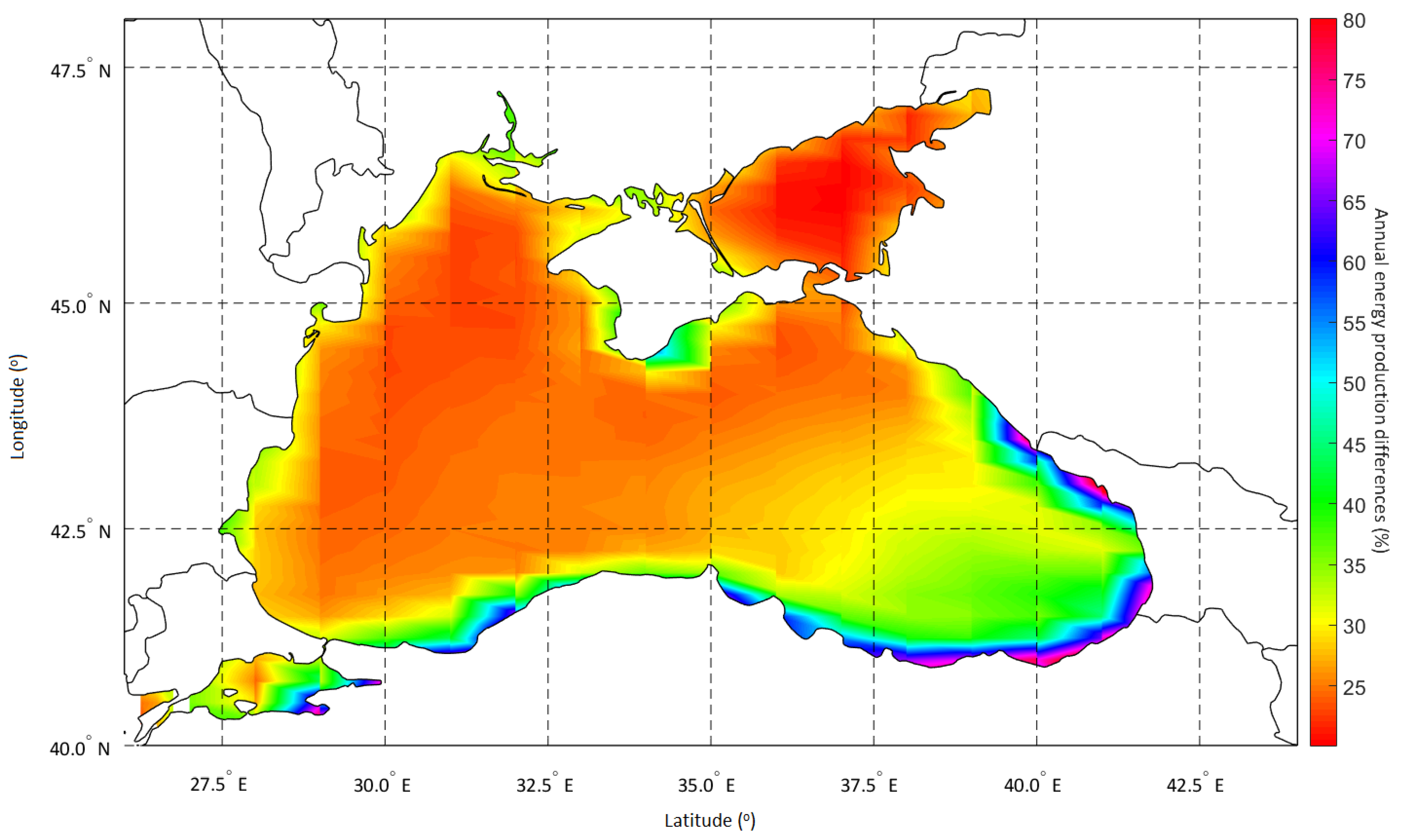
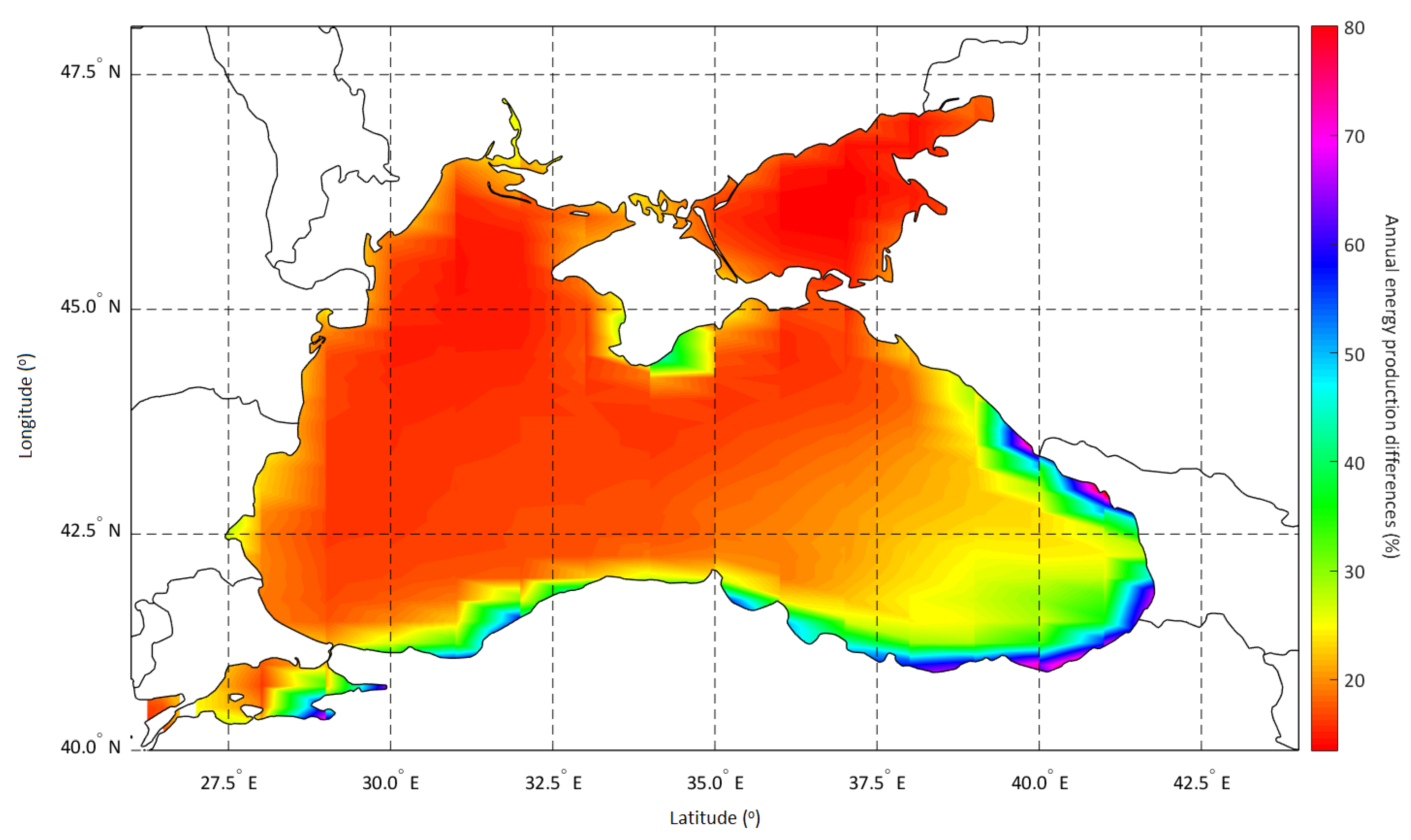
The analysis of Figure 14 and Figure 15 shows that the height at which an AWE is placed has an impact. For a height of 200 m, the system shows a 20% difference compared to a conventional turbine in the Azov Sea and a 22% difference in the western Black Sea. With an increase in height to 414 m, this difference narrows to 13.6% for the Sea of Azov and 14.4% for the west of the Black Sea. This means that, for every 1 m increase in altitude, the difference decreases by approximately 0.04%. To achieve the same AEP value, the optimal AWE 5 MW flight level is in the range of 750–800 m.

By comparing the AEP obtained for the two airborne systems at the height of 200 m with an airborne system of 2 MW, we can identify the superior qualities of the wind for the Black Sea in the Azov region. The 2 MW system studied for a location in Brazil obtained an AEP of 6 GWh with frequent wind speeds of 7 m/s at a height of 255 m [53]. As a result, the 5 MW AWE system registered annual production that was approximately 3 times higher at the height of 200 m. Better values for AEP were obtained near Hawaii at heights of up to 500 m, where a 5 MW AWE has an AEP of approximately 30 GWh [35]. Another study showed that a 1.2 MW AWE operating at altitudes of up to 600 m has production of 3.65 GWh [54] if working in Switzerland, which suggests inferior wind qualities compared to those of the Black Sea.

Although AWEs are still in the pre-commercial phase, they present great advantages regarding cost and the possibility of much easier placement in any location. Furthermore, they do not require expensive foundations like the floating structures for offshore wind turbines, and can be installed on a simple barge in locations with deep water, where ordinary wind turbines cannot be placed yet. Moreover, they can work at different heights so they can be adapted to the height at which the wind speed blows the strongest, which can change from one season to another. Because of lower capacity factors in various geographical areas, until 2030 a 5 MW AWE system will require roughly 18% less capital than a standard wind turbine to provide the same LCOE. The breakeven Capex for speeds between 8 and 12 m/s is approximately 1000 USD/kW, which is 27% less than that of a conventional wind turbine [35]. A project with an AWE of 1–1.5 MW is considered to be implementable until 2030 and, with future studies and attempts at technological improvement, even a 5 MW system is considered feasible [55].

5. Conclusions

In the present work, a complete picture of the Black Sea wind energy potential was provided by taking into account various reference heights and wind turbine technologies. The entire work was based on 20 years of wind data (2002–2011) taken from the ERA5 reanalysis project. In general, this project tends to underestimate the regional wind resources, as highlighted by the comparison with in situ measurements. Although the Black Sea was the target area of this study, it is important to mention that the best wind resources were, in fact, found near the Azov Sea (northern area) regardless of the considered time interval. Nevertheless, taking into account the current geo-political situation, it is difficult to anticipate the implications of a renewable project for this area.

Regarding the Black Sea, the best wind resources were found in the central and western part of this basin, with wind speeds of 8 m/s (U100) expected, in general. Nevertheless, close to the shoreline, only the areas of the west and north are defined by more energetic wind resources. These findings are in line with previous research. The philosophy of the airborne wind systems is to operate at much higher heights (than 100 m), and the comparisons of U100/U500 values showed a difference of 1 m/s for the most energetic areas. In terms of the wind speed and altitude, this difference may not be significant, but for a wind turbine this may lead to better performance since the available power density will increase.

Regarding the wind turbines, all the results were provided in terms of the spatial maps covering the entire Black Sea which, to the best of the knowledge of the authors, may be considered an element of innovation for this area. It is important to mention that no restrictions were included in these maps (i.e., maritime routes, exclusive zones, etc.). From the perception of some reviewers, this may be considered a limitation. The main element of originality is represented by the analysis of the airborne wind systems (500 kW and 5 MW), because this analysis has not previously been carried out for this geographical region (either onshore or offshore). Based on the existing literature, several scenarios were developed in which the optimal altitude flight of the AWES was defined for two particular heights (200 and 414 m). From the comparisons of the 5 MW systems, it is clear that the traditional wind turbine (three blades) provides better performance regardless of the operational heights of the AWES. From a direct comparison (using airborne—U200) of the electricity production, a difference of 22% was found for the western part of the Black Sea, and a maximum of 80% for the eastern area. Nevertheless, similar performance may be expected only in the case when such an AWES can operate at heights exceeding 750 m.

Although the operating principles of the airborne generators are similar, most of the AWESs are still in the early stages of development. In order to become competitive with the traditional wind turbines, these airborne systems need to be capable of improving their capacity production. The scalability process needs to carefully planned since the traction force of the kite will significantly increase, while the overall characteristics of the airborne generator need to be updated. For example, in the work of Dominguez Santana and El-Thalji [56], a 30 kW prototype was upscaled to a 1500 kW version. In this case, the following changes were found: traction force increased from 7.5 to 375 kW; tether diameter increased from 2 to 30 mm; and drum diameter increased from 0.25 to 1.2 m.

Finally, it should be mentioned that the airborne wind market is evolving and may become a serious competitor to the traditional wind turbine, especially in the offshore sector, where large scale systems are expected to be developed that can be easily used for various applications and areas, such as the Black Sea.