Numerical Study of Flat Plate Impact on Water Using a Compressible CIP–IBM–Based Model

Abstract

Due to the entrapment of compressible air, the process of a flat plate impact on water is complicated, which cannot be reproduced using incompressible simulations. To investigate such a slamming process, an accuracy compressible fluid–structure interaction numerical model has been proposed. The solution of this model is based on the constrained interpolation profile (CIP) method to solve the Navier–Stokes equations for the computation of fluid, and an implicit immersed boundary method (IBM) is used to calculate the fluid–structure interaction. Firstly, the present (CIP–IBM–based) model is validated against the problem of the flow past a stationary cylinder. Then it is implemented to simulate the problem of a rigid flat plate impact on water. The predicated impact pressure is compared with reference experiments and other simulations. The CIP–IBM–based model shows a better performance in dealing with sub-atmospheric pressure and reloading. From the numerical view, it is shown that the oscillation of the slamming pressure is significantly affected by the compression and expansion of the entrapped air cushion, and under the influence of the air cushion, the slamming pressure distribution along the bottom is not constant, which also varies greatly with time.

1. Introduction

The process of water entry is a complex multiphase flow problem, which involves gas, liquid and solid. Especially for flat-bottomed structures, different from wedges, cylinder and other structures, an air cushion at the slamming bottom may be entrapped (the compressibility air complicates this problem). As early as the 1960s, Chuang [1], Lewison and Maclean [2] began a series of experimental studies on slamming problems of flat-bottomed structures at small dead-rise angles. Using a high-speed camera [1], it is reported that the existence of air plays a role of cushioning, which reduces the maximum slamming pressure and prolongs the impact time. Experiments by Verhagen [3] pointed out that during the slamming of a flat plate, a sub-atmospheric pressure phenomenon occurred after the maximum pressure. Chuang [4] extended his earlier research to study the slamming problems of elastic flat-bottomed structures. Huang et al. [5] added flanges to the bottom of flat-bottomed structures in experiments. Their results showed that the slamming pressure at the flat bottom could be effectively reduced and tended to be uniform (the slamming pressure has a sharp peak, and the duration of the slamming is very short when there is no flange). However, the total impulse to the structure was not changed.

Lin et al. [6] captured the shape of the water surface with high-speed cameras: when the flat bottom was close to the water surface, a small amount of water–air mixing would appear between the water and the structure. After the bottom entered the water, the mixture would be ejected from both sides. At the meantime, bubbles were formed under the two edges of the bottom, and then small bubbles were generated from the edges to the center. Kang et al. [7] and Oh et al. [8] made a close observation of a flat-bottomed structure slamming process by using a high-speed camera and particle image velocimetry (PIV). The developments of the air pocket in slamming are summarized as three stages: (1) Ripple generation before impact at both edges of the flat bottom; (2) Formation of large air pockets under the bottom during impact; (3) Diminishment of the air pocket. Mayer et al. [9] proposed in more detail through PIV that the large air pocket would first be compressed to the center. They also discussed the development of the jet at both sides of the plate. Ma et al. [10] have compared impact loads between pure and aerated water entry of a flat plate. Although the increasing aeration rate can effectively reduce the peak impact pressure, it has a little effect on total impulse. They have also pointed that there would be a secondary loading after a process of sub-atmospheric pressure. Shin et al. [11] studied the effect of elasticity and plasticity of flat-bottom structures on slamming pressure experimentally. They proposed that the reloading pressure is greatly affected by entrapped air cushion and the elasticity of structure. Mai et al. [12] carried out a series of slamming experiments from low-speed to high-speed plate impact on water, and they pointed out that when the impacting speed is less than 2 m/s, the maximum pressure at the edge of the plate is about 80% of the central pressure; when the impacting speed is greater than 2 m/s, the maximum edge pressure is about 40% of the central pressure.

Referring to the effects of air entrapped on impulsive loading, many studies on wave impact on vertical breakwaters have been conducted. According to Oumeraci et al. [13] and Lugni et al. [14], air entrapped impact is a typical mode of impulsive wave loading. As early as 1939, Bagnold [15] pointed out that the compressibility of air should be considered in the process of a wave impact on a vertical wall. Air pockets between an impinging wave crest and the structure act as cushions, which reduces the impact peak pressure, but also leads to a longer loading period [16,17,18]. Topliss et al. [19] and Hatori et al. [20] pointed out that the air pockets entrapped may cause pressure oscillations after the wave impacting. For caisson breakwaters, Walkden et al. [21] and Buccino et al. [22] recognized that the air entrapped between the overtopping tongue and the structure determines the distribution of maximum pressure or the pressure barycenter.

In recent years, with the improvement of computational efficiency, numerical simulation methods have been applied to the research on the interaction between fluid and coastal structures at different time and space scales [22,23,24,25,26,27]. For floating breakwaters or floating wharfs, more attention needs to be paid to the influence of fluid–structure interaction (FSI) in impulsive loading [25], especially the effect of air entrapment. The research on flat-bottomed structure slamming on water can help to understand the process of wave impact on floating structures (flat plate is an important part of a floating breakwater or wharf). In order to study the mechanism of flat-bottomed structures impact on water, many numerical studies have been carried out. Ng and Kot [28] proposed an incompressible two-phase flow model based on the VOF method to simulate a flat-bottomed structure impact on water. The results showed that the maximum slamming pressure occurred before the bottom had touched the water surface completely. Ma et al. [10,29] established a three-dimensional two-phase flow numerical model for flat plate slamming simulations based on the finite volume method (FVM). Combined with the experimental data, it is proposed that the secondary loading is related to the recompression of the air cushion. Aghaei et al. [30] established a numerical model based on OpenFOAM to study the slamming loads and structural response of elastic plate under water impact.

Commercial CFD software ANSYS Fluent is another numerical tool to study slamming problems caused by flat-bottomed structures. Hu and Liu [31] simulated the flat-bottomed structure slamming on water and pointed out that there is a secondary slamming load in one impacting process, and the second one is greater than the first. The results of Qu et al. [32] showed that when the bottom surface is close to the water, the water surface at the sides is deformed firstly and many bubbles are generated. Yang et al. [33] discussed the influences of flanges to the water impact of an elastic plate.

In the numerical models mentioned above, most of them focused on the comparison and analysis of the maximum slamming pressure. The history of slamming pressure and its relationship with the development of the air cushion are rarely discussed, and there is a little discussion about the sub-atmospheric pressure. The purpose of this paper is to establish a high-order finite difference FSI numerical model and to apply the model to discuss the process of a rigid flat plate impact on water, especially to analyze the correspondence between the slamming pressure and the air cushion.

In this paper, the finite difference method is used to discretize the Navier–Stokes (N–S) equations, in which the advection term is discretized by the constrained interpolation profile (CIP) method. In the CIP method, the physical value and its spatial derivatives are computed at the same time, and it has the advantages of high-order numerical accuracy and sub-cell resolution [34,35]. Hu and Kashiwagi [36], He [37], Ji et al. [38] and Wang et al. [39] have fully applied the CIP method in incompressible fluid–structure interaction simulations. Hu and Kashiwagi [36], Yang and Qiu [40] and Sun et al. [41] introduced the CIP method to deal with compressible flow problems. Yang and Qiu [40] calculated the problem of water entry of wedges. Their results are in good agreement with experimental data. In contrast to Yang and Qiu [40], the tangent of hyperbola for interface capturing (THINC) scheme is chosen to compute the free surface [42], and for the FSI term, the implicit immersed boundary method (IBM) is used. In the IBM, in order to guarantee no-slip boundary conditions, the solid structures are treated as a force source term to the fluid. This method is based on Cartesian mesh, which avoids the use of body-fitted meshes, and it has the advantage of ensuring the accuracy without increasing the calculation [43,44]. Compared with the traditional IBM, the implicit IBM improves the accuracy [45], which would be discussed in the section of solver validation.

This paper is structured as follows: firstly, the numerical model is introduced in detail, and then this model is validated against the problem of the flow past a stationary cylinder. Special attention is paid to the problem of a flat plate impact on water. After comparing the numerical results with the experimental data, the history and distribution of impact pressure along the bottom of the plate are analyzed. The relationship between the pressure and the air cushion is discussed in detail. Summary and conclusions are given in the last section.

In this paper, FORTRAN programming language was used for calculations.

2. Numerical Model

2.1. Governing Equations

Firstly, the whole calculation domain is assumed to be a compressible viscous two-phase flow, and the energy equation is not considered. The continuity equation and Navier–Stokes (N–S) equations are chosen:

$$\frac{\partial \rho }{\partial t}+\nabla ·\left(\rho u\right)=0$$

(1)

$$\frac{\partial u}{\partial t}+\left(u·\nabla \right)u=\mathrm{g}+f-\frac{1}{\rho }\nabla p+\frac{\mu }{\rho }{\nabla }^{2}u$$

(2)

where $\rho$ is the density, $t$ is the time, $u$ is the velocity, $\mathrm{g}$ is the gravity and $f$ is the force source term, which means the external force subjected by the solid body. The sound speed definition is chosen as a relationship between $\rho$ and $p$:

$$C_s=\sqrt{dp/d\rho }$$

(3)

In Equation (3), $C_s$ is the speed of sound. Combine Equation (1) with Equation (3):

$$\frac{\partial p}{\partial t}+u·\nabla p=-\rho C_s^2\nabla ·u$$

(4)

Equations (1), (2) and (4) constitute the governing equations.

For the two-phase flow, the function ${\phi }_m$ is chosen as the volume fraction for each phase in the computational grid, in which the volume function of the liquid ${\phi }_1$ is solved as follows:

$$\frac{\partial {\phi }_1}{\partial t}+\left(u·\nabla \right){\phi }_1=0$$

(5)

The tangent of hyperbola for interface capturing (THINC/SW) method is adopted to solve this equation, which is a high accuracy VOF-type method [42]. In this paper, the solid is treated as rigid, so the solid phase ${\phi }_3$ is solved automatically by the proportion of the solid boundary in the computational grid. The gas phase is calculated as follows:

$${\phi }_2=1-{\phi }_1-{\phi }_3$$

(6)

Then the physical property can be determined by the volume fraction: $\lambda ={\phi }_1{\lambda }_1+{\phi }_2{\lambda }_2+{\phi }_3{\lambda }_3$, where the $\lambda$ can represent the density $\rho$, the viscosity $\mu$ (to ensure the stability of the calculation, the viscosity of the solid phase is set the same as the liquid phase) or the velocity of sound $C_s$. The stiffened gas equation of state is used to calculate the velocity of sound in water ($C_1$) and in air ($C_2$) [41]: $C_i=\sqrt{\gamma \left(P_0+\kappa \right)/{\rho }_0}$, where $P_0$ denotes standard atmospheric pressure, ${\rho }_0$ is the initial density of each phase. In this paper, the properties of $\gamma$ and $\kappa$ are set as 1.4 and 0.0 Pa in the air phase and 7.15 and 308 Mpa in the water phase.

2.2. Numerical Methods

According to the projection method, the continuity equation and the N–S equation without the force source term are solved based on the CIP method firstly, and then the the IBM is used to solve the force source term and to renew the velocity, which is influenced by the rigid body.

2.2.1. CIP-Based Flow Solver

Firstly, the solution of Equation (1), Equation (2) without the force source term and Equation (4), are divided into three parts [34,35,36]:

(I)

Advection term:

$$\frac{\partial \rho }{\partial t}+\left(u·\nabla \right)\rho =0$$

(7)

$$\frac{\partial u}{\partial t}+\left(u·\nabla \right)u=0$$

(8)

$$\frac{\partial p}{\partial t}+\left(u·\nabla \right)p=0$$

(9)

The CIP method is used to solve the advection term. The detailed steps are referred to in references [35,36]. After this step, the intermediate values are obtained: $u^{*}$, ${\rho }^{*}$ and $p^{*}$.

(II)

Diffusion term:

$$\frac{\partial u}{\partial t}=\mathrm{g}+\frac{\mu }{\rho }{\nabla }^{2}u$$

(10)

Equation (10) is solved by the central difference scheme in the spatial step and the intermediate velocity $u^{**}$ is obtained.

(III)

Pressure term:

$$\frac{\partial \rho }{\partial t}=-\rho \nabla ·u$$

(11)

$$\frac{\partial u}{\partial t}=-\frac{1}{\rho }\nabla p$$

(12)

$$\frac{\partial p}{\partial t}=-\rho C_s^2\nabla ·u$$

(13)

Take the divergence of Equation (12) and combine Equation (13), we get the following Poisson-type equation of pressure:

$$\frac{\partial }{\partial x_i}\left(\frac{1}{\rho }\frac{\partial p^{n+1}}{\partial x_i}\right)=\frac{p^{n+1}-p^{*}}{{\rho }^{*}{C}_s^2∆t^2}+\frac{1}{∆t}\frac{\partial u_i^{**}}{\partial x_i}$$

(14)

Equation (14) is solved by the successive over relaxation (SOR) iterative method. The velocity $u^{n+1/2}$ and density ${\rho }^{n+1}$ can be further obtained by means of the pressure values.

Then, add the force source term, update the velocity to the next time step:

$$\frac{u^{n+1}-u^{n+1/2}}{∆t}=f$$

(15)

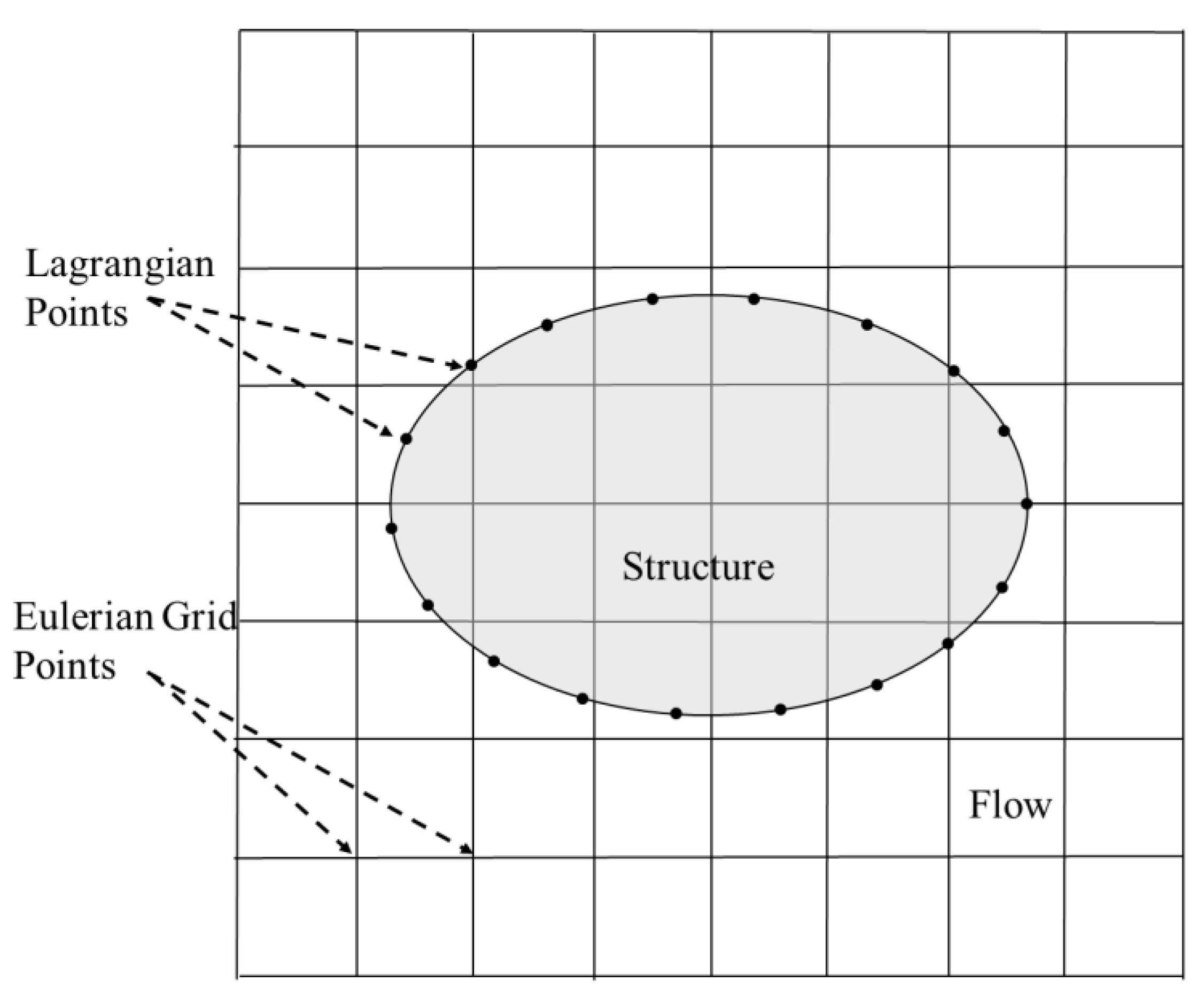
2.2.2. Implicit IBM Method

In this paper, the velocity correction is based on the implicit IBM [45]. Form Equation (15),

$$u^{n+1}=u^{n+1/2}+∆u$$

(16)

where the speed correction is $\mathsf{\Delta }u=f\mathsf{\Delta }t$. As shown in Figure 1, the idea of the IBM is to disperse the forces on the Lagrangian points to the Eulerian grid points, using the Dirac function. With this method, the fluid at the boundary of the structure satisfies the no-slip boundary conditions.

For the fluid domain, the velocity of n + 1/2 step at the Lagrangian points needs to be corrected so that it is equal to the boundary velocity. Assuming that the correction at the boundary points in the fluid is an unknown velocity value $\mathsf{\Delta }{u}_B$, then the velocity acting on the Eulerian grid points is corrected to:

$$\Delta u={\int }_{\mathsf{\Gamma }}\Delta u_B·\delta \left(x-X_B\right)ds$$

(17)

where x means the fluid domain in the Eulerian grid, and X means the motion of the solid body in the Lagrangian coordinate, $\delta \left(x-X_B\right)$ is the Dirac function, ds is the distance of Lagrangian points on the structure. In this paper, referring to Peskin [44], the following expression about the Dirac function is given:

$$\delta \left(x\right)\approx {\delta }_h\left(x\right)=\frac{1}{∆x∆y}\varphi \left(\frac{x}{∆x}\right)\varphi \left(\frac{y}{∆y}\right)$$

(18)

where the function $\varphi$ can be expressed as:

$$\varphi \left(r\right)=\{\begin{array}{cc}\hfill \left(3-2\left|r\right|+\sqrt{1+4\left|r\right|-4r^2}\right)/8,\hfill & \hfill \left|r\right|\le 1\\ \hfill \left(5-2\left|r\right|+\sqrt{-7+12\left|r\right|-4r^2}\right)/8,\hfill & \hfill 1<\left|r\right|\le 2\\ \hfill 0,\hfill & \hfill \left|r\right|>2\end{array}$$

(19)

In order to satisfy the non-slip boundary condition, the corrected velocity on the Eulerian grid is interpolated back to the rigid body boundary point again, and its value is equal to the velocity at the boundary:

$$U_B={\int }_{\mathsf{\Omega }}{u}^{n+1}\delta \left(x-X_B\right)d\mathsf{\Omega }$$

(20)

where $U_B$ is the velocity at the boundary of the rigid body. By taking Equations (16) and (17) into Equation (20), we can get a set of equations to solve the unknown value ∆u_B:

$$U_B={\int }_{\mathsf{\Omega }}(u^{n+1/2}+{\int }_{\mathsf{\Gamma }}∆u_B·\delta \left(x-X_B\right)ds)\delta \left(x-X_B\right)d\mathsf{\Omega }$$

(21)

By solving Equation (21), we can get the velocity correction $\mathsf{\Delta }{u}_B$, and then the updated velocity $u^{n+1}$ on the Eulerian grid can be obtained by using Equations (17) and (16).

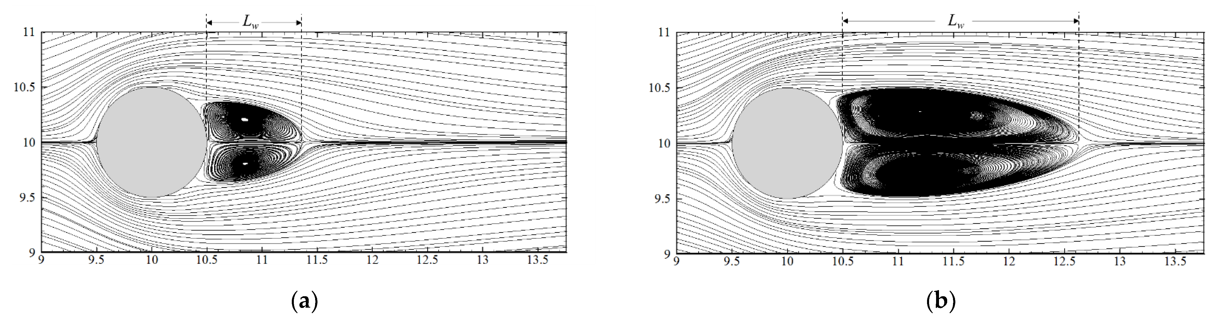
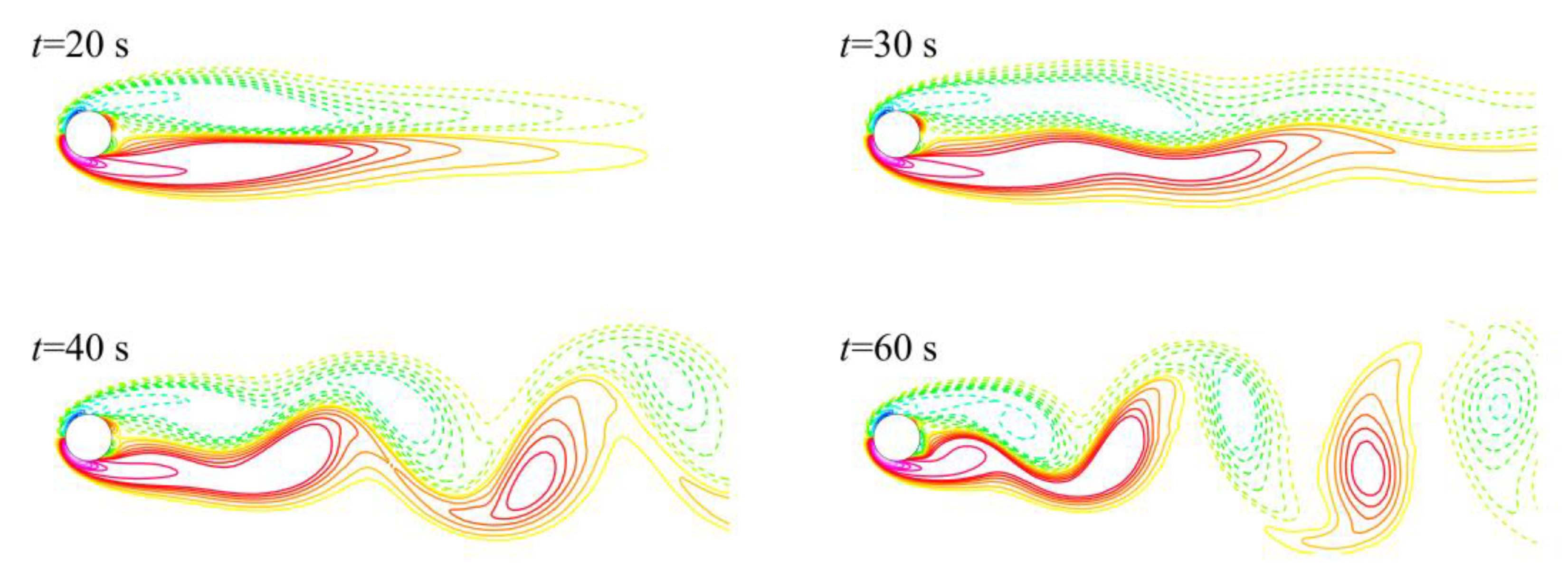
3. Solver Validation: 2D Flow Past a Stationary Cylinder

In order to validate the solver described above, the model is first applied to simulate the problem of 2D flow past a stationary cylinder. The calculation area is shown in Figure 2a, where the diameter of the cylinder is D. The left side is the inflow boundary, and the inflow velocity is $U_{\infty }$; the right side is the open boundary; and the top and bottom sides are treated as the slip boundary condition. As shown in Figure 2b, the variable grids are used in the computation with the refined meshes near the cylinder. The spacing of the Lagrange nodes is consistent with that of the Euler gird nearby.

Two steady and an unsteady flow past a stationary cylinder are simulated, in which the Reynolds numbers are 20, 40 and 100. The Reynolds number is defined as:

$$Re=\frac{\rho U_{\infty }D}{\mu }$$

(22)

In the present simulations, three different sizes of mesh are chosen. The minimum gird is ∆x = ∆y = 0.04 D, ∆x = ∆y = 0.02 D and ∆x = ∆y = 0.01 D, respectively. The drag and lift coefficients and the Strouhal number are chosen to compare with other methods. The drag coefficient C_d and the lift coefficient C_l are defined as:

$$C_d=\frac{2F_d}{\rho U_{\infty }{}^{2}D},C_l=\frac{2F_l}{\rho U_{\infty }{}^{2}D}$$

(23)

The drag force F_d and lift force F_l can be calculated by

$$F_i={\int }_{\mathsf{\Gamma }}\left[-p{\delta }_{ij}+\mu \left(\frac{\partial u_i}{\partial x_j}+\frac{\partial u_j}{\partial x_i}\right)\right]n_{j}ds$$

(24)

When the flow is unstable, the vortices behind the cylinder will move downstream and shed with the frequency f_s. The Strouhal number S_t is a dimensionless vortex shedding frequency which is defined as:

$$S_t=\frac{fD}{U_{\infty }}$$

(25)

First, the steady flows at Re = 20 and 40 past a cylinder are simulated. The comparison results (the drag coefficient C_d and the length of wake L_w) are listed in

Table 1. Comparison of the drag coefficient and the length of steady state wake for Re = 20 and Re = 40.

	Re = 20		Re = 40
	Cd	Lw/D	Cd	Lw/D
$\mathrm{Present}∆x=∆y=0.04D$	2.20	0.99	1.65	2.37
$\mathrm{Present}∆x=∆y=0.02D$	2.17	0.92	1.62	2.20
$\mathrm{Present}∆x=∆y=0.01D$	2.14	0.89	1.60	2.14
Tritton (1959) [46]	2.09	-	1.59	-
Coutanceau and Bouard (1977) [47]	-	0.93	-	2.13
Ye et al. (1999) [48]	2.03	0.92	1.52	2.27
Taira and Colonius (2007) [49]	2.06	0.94	1.54	2.30
Horng et al. (2018) [50]	2.10	0.93	1.56	2.18

, where the studies of Tritton [46] and Coutanceau and Bourand [47] are based on experiments. The numerical results based on the CIP–IBM method have good convergence. Especially when the Reynolds number is 40, as shown in Table 1, the drag coefficient C_d of the experiment is 1.59, while the results based on the fine mesh is 1.60. The experiment’s lift coefficient C_l is 2.13, and the numerical simulation is 2.14. The present numerical results based on the fine grid are closer to the experiments than the others [48,49,50]. Figure 3 shows the streamlines near the cylinder ($∆x=∆y=0.01D$). Two symmetrical wake vortices are formed behind the cylinder, and the vortex has a larger length when the Reynolds number is greater.

Then, we consider the unsteady flow past a cylinder for Re = 100.

Table 2. Comparison of drag and lift coefficients, and Strouhal number of flow past the cylinder for Re = 100.

	${\overline{\mathit{C}}}_{\mathit{d}}$	${\mathit{C}}_{\mathit{d}}^{\prime }$	${\mathit{C}}_{\mathit{l}}^{\prime }$	${\mathit{S}}_{\mathit{t}}$
$\mathrm{Present}∆x=∆y=0.04D$	1.433	$\pm$0.012	$\pm$0.312	0.161
$\mathrm{Present}∆x=∆y=0.02D$	1.409	$\pm$0.013	$\pm$0.318	0.165
$\mathrm{Present}∆x=∆y=0.01D$	1.395	$\pm$0.013	$\pm$0.322	0.167
Liu et al. (1998) [51]	1.350	$\pm$0.012	$\pm$0.339	0.165
Lai and Peskin (2000) [43]	1.447	-	$\pm$0.330	0.165
Uhlmann (2005) [52]	1.453	$\pm$0.011	$\pm$0.339	0.169
Yu and Shao (2007) [53]	1.394	$\pm$0.009	$\pm$0.316	0.174
Di and Ge (2015) [54]	1.385	$\pm$0.009	$\pm$0.344	0.168
Horng et al. (2018) [50]	1.40	-	$\pm$0.36	0.170

shows the comparison of the computed drag and lift coefficients and the Strouhal number with others’ simulations. Liu et al.’s results are based on the body-fitted grid method [51], and the other results are all based on the different immersed boundary method. It is revealed that the mean drag coefficients (${\overline{C}}_d$) calculated by Lai and Peskin [43] and Uhlmann [52] based on the traditional IBM method are higher than those based on the body-fitted grid method. The direct-forcing immersed boundary method (IBM) is used by Yu and Shao [53], Di and Ge [54] and Horng et al. [50], which shows better agreement with the result of Liu et al. [51]. The present method converges fast, and its accuracy is close to the direct-forcing IBM. The calculation results show that the fine grids ($∆x=∆y=0.01D$) are the optimal choice. Based on the fine grids, Figure 4 gives the time history of the drag and lift coefficient, and Figure 5 shows the time evolution of the vorticity contours around the cylinder of the present method for Re = 100. In the simulations, after a short time of the uniform flow, the vortex shedding shows gradually due to the increase in the asymmetric body force. The present numerical simulation reproduces the periodic vortex shedding, forming the Kármán vortex street (Figure 5 t = 60 s).

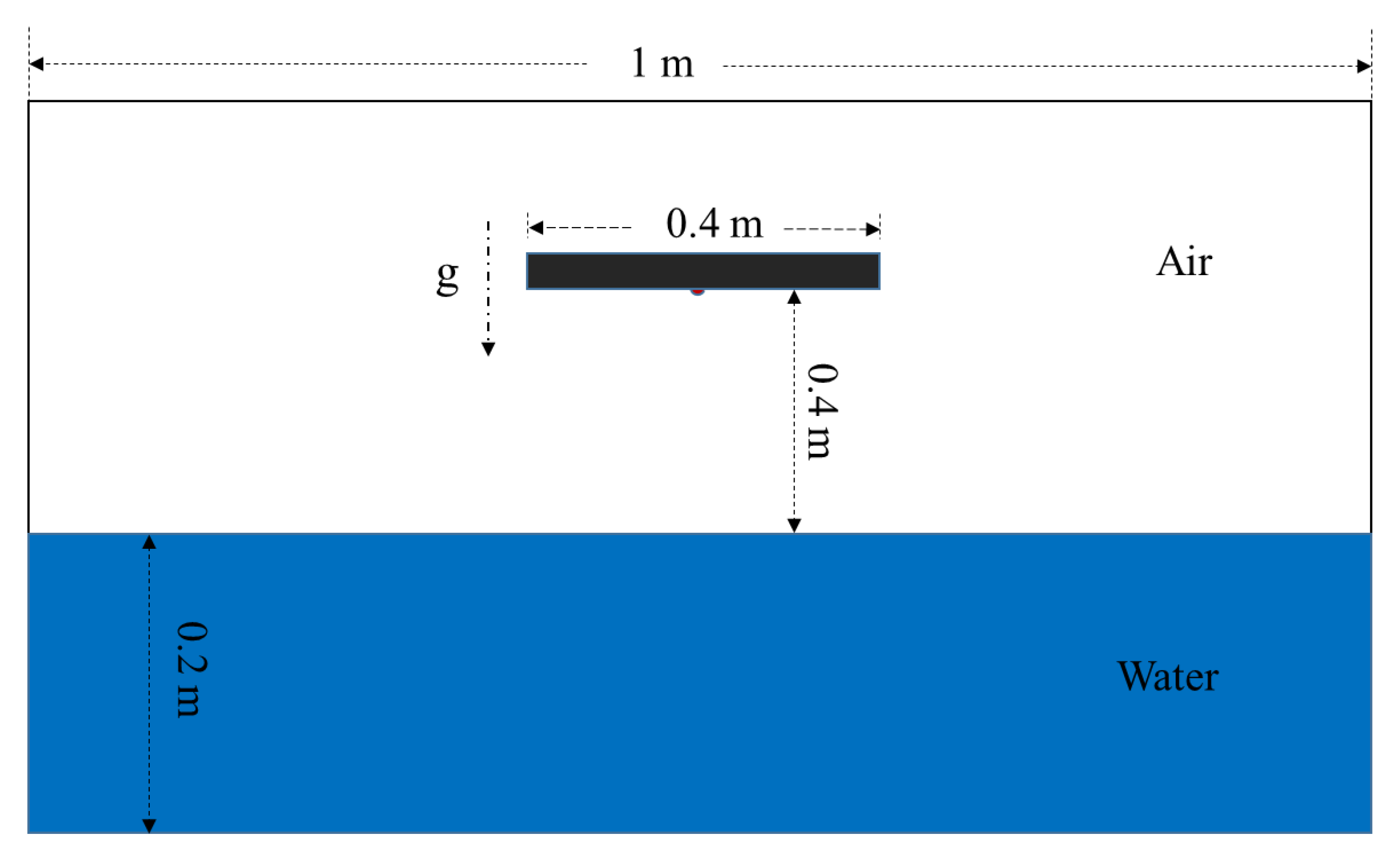
4. Simulation and Analysis of 2D Flat Plate Impact on Water

4.1. Equation of Body Motion

In this paper, the movement of each point is the same, because the plate is rigid and the movement is translation (not rotation). The plate is only affected by the gravity and the force of the fluid, so the equation of the body motion is calculated as follows:

$$\frac{dR}{dt}=U_B$$

(26)

$$\frac{d{U}_B}{dt}=\mathrm{g}+\frac{F}{M}$$

(27)

where R is the displacement of the plate; M is the mass of structure; F is the force of the fluid acting on the structures and it can be calculated using Equation (24). According to Gauss’s theorem, Equation (24) can be transformed into:

$$F_i=-{\int }_{\mathsf{\Omega }}\frac{\partial p}{\partial x_i}{\phi }_{3}d\mathsf{\Omega }+\mu {\int }_{\mathsf{\Omega }}\frac{\partial }{\partial x_i}\left(\frac{\partial u_i}{\partial x_j}+\frac{\partial u_j}{\partial x_i}\right)d\mathsf{\Omega }$$

(28)

Because the rotation and deformation of the object are not taken into account, $U_B$ is both the internal and boundary velocity of the plate. By taking $U_B$ to Equation (21), combining Equations (16) and (17), the updated flow velocity $u^{n+1}$ can be obtained. Then $u^{n+1}$ and $p^{n+1}$ are taken into Equation (28) to obtain the force $F^{n+1}$ of the fluid acting on the structure. In the next step of time (n + 2), bring the force $F^{n+1}$ into Equation (27), and the velocity of the plate in new step can be obtained.

4.2. Description and Comparison

The two-dimensional water entry model used in this paper refers to the experiment of Verhagen [3]. Initially, as shown in Figure 6, the water is still, and a flat plate (0.4 m in width) is floating above the water surface. Suddenly, the plate drops to the water because of gravity, so the impacting velocity is 2.8 m/s. There is a pressure gauge located in the center of the bottom of the plate. In order to reduce the calculation time, the calculated area is set to 1.0 m in width and 0.6 m in height, in which the height of the air zone is 0.4 m and the water is 0.2 m in depth. The density of the water is 1000 kg/m³, and 1.29 kg/m³ for the air. In this paper, the thickness of the plate is set as 0.03 m, and the density of the plate in this simulation is 2500 kg/m³. The background pressure in the calculation region is set as 10⁵ Pa. Uniform meshes are chosen: from Δx = Δy = 8 mm to Δx = Δy = 2 mm; and the spacing of Lagrangian points is the same as the distance of the grids, from Δs = 8 mm to Δs = 2 mm; the time step is all set as Δt = 5 × 10⁻⁶ s (according to Yang and Qiu [40], they set Δt = 5.7 × 10⁻⁶ s).

Figure 7 is a comparison of the present numerical results with the experimental data [3], Yang and Qiu’s results [40] based on the CIP method and the results of Ma et al. [29] based on the finite volume method. When the girds get finer, the numerical simulations are close to the experimental data at Δx = Δy = Δs = 2 mm. As shown in Figure 7, during the slamming, the pressure at the bottom center increases rapidly, reaching the maximum value (3.5 × 10⁵ Pa) in a short time, and then the pressure decreases immediately, resulting in a negative (sub-atmospheric) pressure of about −1.5 × 10⁵ Pa. After that, a secondary loading pressure, which is much smaller than the first maximum, appears and then the pressure continues to oscillate around zero for a period. It can be seen from the comparison in the figure that the simulation of the three numerical results for the maximum slamming pressure are all consistent with the experimental data. But for the negative pressure, the results of the CIP–IBM method proposed in this paper are closer to the experimental data, and the CIP–IBM method also shows a better trend process for the subsequent rise of the pressure, which reaches a secondary slamming pressure peak. The secondary loading value of the CIP–IBM numerical simulation is slightly higher than the experimental results. The reason for this difference may be that the compression of the air cushion at the bottom of the flat plate in the two-dimensional numerical simulation is more violent than that in the three-dimensional experiment.

In order to clarify the relationship between the slamming pressure and the air cushion, the synchronous duration curve of the volume of the entrapped air pocket (Vair) and the slamming pressure is given in Figure 8. As the slamming pressure increases rapidly, the volume of the entrapped air decreases rapidly. When the slamming pressure reaches the maximum, the volume of the air cushion at the bottom also reaches the minimum. After that, the pressure gradually decreases with the increase in the entrapped air volume. When the air cushion expands to the maximum, the maximum negative pressure value appears at the bottom of the plate. It can also be seen from the subsequent time histories (Figure 8) that the oscillation of the slamming pressure and the change of the entrapped air volume are inversely synchronized.

4.3. Evaluation of Water Surface and Air Cushion during Slamming

Figure 9a–f show the changes of the free surface and the corresponding flow field during the water entry slamming, and the formation and development of the air cushion at the bottom of the flat plate can also be observed. Take φ = 0.5 as the interface between water and air, and the moment when the slamming pressure reaches the maximum is recorded as t₀ (as shown in Figure 7). Figure 9a shows that at t₀ − 1 ms, when the plate is just touching the water surface at t₀ − 1 ms, there is an air layer entrapped. This air layer is similar to an air cushion (it is thick in the middle and thin at both sides). In the meantime, due to the influence of the rapid airflow, the water surface under the sides of the plate is rippling, which is consistent with the phenomenon observed in the experiments of Kang et al. [7] and Oh et al. [8].

Figure 9b–f correspond to the moment of t₀ to t₄ (as can be seen in Figure 7 and Figure 8), respectively. As shown in Figure 9b, when the slamming pressure reaches the maximum at t₀, the air layer under the bottom of the plate almost disappears, and only a tiny gas–liquid mixture remains in the center of the plate. At this moment, when the plate is in parallel contact with the water surface, the slamming pressure comes to the maximum, and the air flow at both sides becomes more violent, thereby generating two small air pockets, and the jet flow begins to form near the edges of the plate. The slamming pressure drops rapidly after reaching its maximum value to zero (standard atmospheric pressure) after 0.8 ms. As can be seen in Figure 9c, a thin air cushion appears at the bottom of the plate. At this time (t₁), the jets at both sides of the plate continue to develop, and the pockets under the edges of the plate become bigger. At t₂ (t₀ + 1.7 ms), the slamming pressure reaches its minimum (a negative pressure). As shown in Figure 9d, the air cushion at the bottom of the plate is obviously expanded as compared with the moment of t₁ (Figure 9c). The shape of the air cushion is visible: thick in the middle and thin at both edges. The expansion process of the air cushion can be clearly observed from Figure 9b–d, and the corresponding slamming pressure changes from the maximum to the zero, and then to the negative pressure (the minimum). Combined with the analysis in Figure 8, it is inferred that the decrease in the pressure, especially the reason of the negative pressure, is due to the expansion of the air cushion at the bottom.

From t₂ to t₃, the slamming pressure rises from the negative value to a secondary peak. In Figure 9e, during the moment of t₃ (t₀ + 3.2 ms), compared with t₂, the thickness of the air cushion at the bottom of the plate does not change obviously. However, the air cushion tends to be compressed toward the center, which is consistent with the PIV test results of Mayer et al. [9]. The continued drop of the plate and the compression of the air cushion to the center are the main reasons for the rise of the pressure. It can be seen from Figure 7 that the rise of pressure reaches a secondary peak, which is consistent with the experimental and numerical analysis of Ma et al. [10]. In this stage, clear jets appear on both sides, and the air pockets under the two edges of the plate become more obvious. At t₄ (t₀ + 4.05 ms), as shown in Figure 9f, the air cushion at the center of the bottom tends to expand again, and the slamming pressure is lower than the moment of t₃. Due to the existence of the air cushion under the bottom of the plate, the slamming pressure fluctuates near zero for a short period of time.

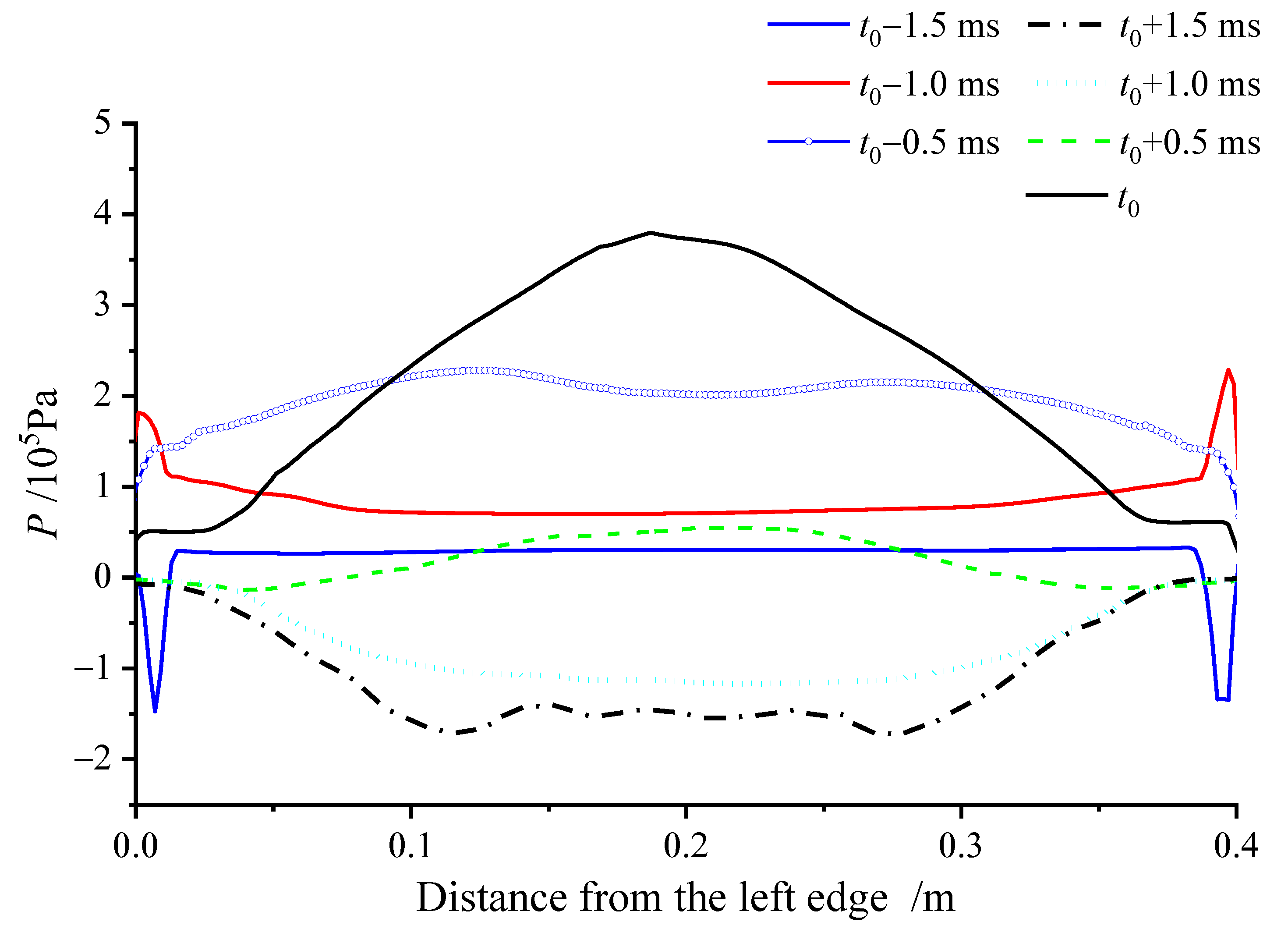
4.4. Distribution of the Slamming Pressure

As shown in the previous section, the pressure at the bottom of the flat plate is affected by the air cushion during slamming. In addition, the presence of the air cushion causes an unbalanced distribution of the slamming pressure along the bottom. Figure 10 shows the slamming pressure at different positions. The closer to the bottom center, the greater the maximum slamming pressure is. When the distance from the center is 15 cm, the maximum slamming pressure is only 1.5 × 10⁵ Pa, which is about 40% of the maximum at the center point (the result is consistent with the experiment of Mai et al. [12]). In the subsequent negative pressure values, the results of the center point and its vicinity (5 cm) are close. Compared with Figure 9d, we can see that both the two points are in the expanded air cushion, and the expansion of the air cushion is the cause of the negative pressure. The farther away from the center, the weaker the air cushion effect is, and the less obvious the negative pressure is. The pressure rises again, and the appearance of the secondary peak value also indicates that it has the effect of the air cushion: the secondary maximum pressure values near the center are greater and appear later.

Figure 11 shows the distribution of the pressure at the bottom at different times during the flat plate impact on water. At the moment of t₀ − 1.5 ms, the plate is approaching to water surface, and the pressure at the bottom of the plate is the same, which is about 0.3 × 10⁵ Pa. However, the parts under both edges of the plate are affected by the airflow, which results in negative pressure, and the negative pressure drops to −1.5 × 10⁵ Pa. At t₀ − 1.0 ms, the pressure at the bottom increases slightly when the plate starts to touch the water surface. The increase in the pressure at the center is less due to the influence of the air cushion, while much greater changes affected by the air flow have happened at both edges of the plate. After 0.5 ms (at t₀ − 0.5 ms), the pressure at the bottom of the plate continues to increase, over 2.0 × 10⁵ Pa. The pressure at both edges is much smaller than that in the middle, and it can be seen that, due to the air cushioning effect, the pressure at the center of the plate is slightly smaller than that beside the center. When the slamming pressure reaches the maximum (the moment of t₀), the air cushion is compressed completely. The distribution of the pressure decreases from the center to both sides. At t₀ + 0.5 ms, the pressure at the bottom decreases rapidly, and the trend is higher at the center than the edges. The maximum pressure drops to 0.5 × 10⁵ Pa. At the moment of t₀ + 1.0 ms and t₀ + 1.5 ms, the expansion of the air cushion causes negative pressures, and the pressure at both edges of the plate is about zero, where there is no gas involved. The pressure distribution at the bottom also shows that the negative pressure in the central part is lower than that at the edges.

5. Conclusions

A numerical model of fluid–structure interaction based on the CIP–IBM method is proposed. The CIP method is adopted to discretize the N–S equations, which has the advantages of high accuracy and low dissipation. An implicit IBM method is introduced to calculate the fluid–structure interaction. This method is based on the Cartesian grid, which reduces the complexity of the body-fitted meshes.

The CIP–IBM method is validated by computing the flow past a stationary cylinder. It shows better outcomes than the traditional IBM method. Then the present model is applied to simulate the problem of a rigid flat plate impact on water. It simulates the maximum slamming pressure accurately and shows a trend closer to the experimental data than the previous numerical simulations, especially the negative pressure and the secondary maximum. This suggests that the CIP–IBM method can be used to simulate the FSI problems effectively.

Finally, detailed discussions are presented based on the simulation: when the flat plate impacts on water, there is an air cushion generated at the bottom, and the air cushion is compressed rapidly. At the same time, the pressure at the bottom center reaches the maximum. The peak pressure decreases from the center to the edges. After that, the air cushion expands and the pressure at the bottom drops to the minimum (a negative pressure value). After quantitative analysis of the relationship between the air volume and the slamming pressure, it is considered that the negative pressure is mainly caused by the expansion of the air. Then, due to the continued movement of the plate, the air cushion will be compressed to the center. The slamming pressure rises again, resulting in a reloading pressure peak. Subsequently, the air cushion at the bottom of the plate causes the slamming pressure to oscillate slightly near zero.

Under the influence of the air cushion, the distribution of the slamming pressure at the bottom is complicated. The central part changes violently and the changes at both edges are smaller. The results have also shown that, due to the movement of the air, ripples and jets are generated successively on the water surface near both edges of the plate.

References

1. Chuang, S.L. Experiments on flat-bottom slamming. J. Ship Res. 1966, 10, 10–27. [Google Scholar] [CrossRef]
2. Lewison, G.; Maclean, W.M. On the cushioning of water impact by entrapped air. J. Ship Res. 1968, 12, 116–130. [Google Scholar] [CrossRef]
3. Verhagen, J.H.G. The impact of a flat plate on a water surface. J. Ship Res. 1967, 11, 211–223. [Google Scholar] [CrossRef]
4. Chuang, S.L. Investigation of impact of rigid and elastic bodies with water. In Naval Ship Research and Development Center Report 3248; Defense Technical Information Center: Fort Belvoir, VA, USA, 1970. [Google Scholar]
5. Huang, Z.Q.; Zhang, W.H. Experimental investigation on the reduction of flat-bottom body slamming. Huazhong Univ. Sci. Technol. 1986, 14, 725–730. (In Chinese) [Google Scholar]
6. Lin, M.C.; Shieh, L.D. Simultaneous measurements of water impact on a two-dimensional body. Fluid Dyn. Res. 1997, 19, 125–148. [Google Scholar] [CrossRef]
7. Kang, H.D.; Oh, S.H.; Kwon, S.H.; Chung, J.-Y.; Jung, K.H.; Jo, H.J. An experimental study of shallow water impact. In Proceedings of the 23rd International Workshop on Water Waves and Floating Bodys, Jeju, Korea, 13–16 April 2008. [Google Scholar]
8. Oh, S.H.; Kown, S.H.; Chung, J.Y. A close look at air pocket evolution in flat impact. In Proceedings of the 24th International Workshop on Water Waves and Floating Bodys, Zelenogorsk, Russia, 19–20 April 2009. [Google Scholar]
9. Mayer, H.C.; Krechetnikov, R. Flat plate impact on water. J. Fluid Mech. 2018, 850, 1066–1116. [Google Scholar] [CrossRef] [Green Version]
10. Ma, Z.H.; Causon, D.M.; Qian, L.; Mingham, C.G.; Mai, T.; Greaves, D.; Raby, A. Pure and aerated water entry of a flat plate. Phys. Fluids 2016, 28, 016104. [Google Scholar] [CrossRef] [Green Version]
11. Shin, H.; Seo, B.; Cho, S.R. Experimental investigation of slamming impact acted on flat bottom bodies and cumulative damage. Int. J. Nav. Archit. Ocean Eng. 2018, 10, 294–306. [Google Scholar] [CrossRef]
12. Mai, T.; Mai, C.; Raby, A.; Greaves, D. Aeration effects on water-structure impacts: Part 1. Drop plate impacts. Ocean Eng. 2019, 193, 106600. [Google Scholar] [CrossRef]
13. Oumeraci, H.; Klammer, P.; Partenscky, H.W. Classification of breaking wave loads on vertical structures. J. Waterw. Port Coast. Ocean Eng. 1993, 119, 381–397. [Google Scholar] [CrossRef]
14. Lugni, C.; Brocchini, M.; Faltinsen, O.M. Wave impact loads: The role of the flip through. Physic Fluids 2006, 18, 1473–1486. [Google Scholar] [CrossRef]
15. Bagnold, R. Interim report on wave-pressure research. J. Inst. Civ. Eng. 1939, 12, 201–226. [Google Scholar] [CrossRef]
16. Takahashi, S.; Tanimoto, K.; Miyanaga, S. Uplift wave forces due to compression of enclosed air layer and their similitude law. Coast. Eng. J. 1985, 28, 191–206. [Google Scholar] [CrossRef]
17. Cooker, M.J.; Peregrine, D.H. Computation of violent motion due to waves breaking against a wall. In Proceedings of the 22nd International Conference on Coastal Engineering, ASCE, Delft, The Netherlands, 29 January 1990; pp. 164–176. [Google Scholar]
18. Kirkgoz, M.S. Impact pressure of breaking waves on vertical and sloping walls. Ocean Eng. 1991, 18, 45–59. [Google Scholar] [CrossRef]
19. Topliss, M.E.; Cooker, M.J.; Peregrine, D.H. Pressure oscillations during wave impact on vertical walls. In Proceedings of the 23rd Coastal Engineering Conference, Venice, Italy, 4–9 October 1992; pp. 1639–1650. [Google Scholar]
20. Hattori, M.; Arami, A.; Yui, T. Wave impact pressure on vertical walls under breaking waves of various types. Coast. Eng. 1994, 22, 79–114. [Google Scholar] [CrossRef]
21. Walkden, M.J.; Wood, D.J.; Bruce, T.; Peregrine, D.H. Impulsive seaward loads induced by wave overtopping on caisson breakwaters. Coast. Eng. 2001, 42, 257–276. [Google Scholar] [CrossRef]
22. Buccino, M.; Daliri, M.; Dentale, F.; Calabrese, M. CFD experiments on a low crested sloping top caisson breakwater. Part 2. Analysis of plume impact. Ocean Eng. 2019, 173, 345–357. [Google Scholar] [CrossRef]
23. Liu, S.; Gatin, I.; Obhrai, C.; Ong, M.C.; Jasak, H. CFD simulations of violent breaking wave impacts on a vertical wall using a two-phase compressible solver. Coast. Eng. 2019, 154, 103564. [Google Scholar] [CrossRef]
24. Gao, J.L.; Ma, X.Z.; Zang, J.; Dong, G.H.; Ma, X.J.; Zhu, Y.; Zhou, L. Numerical investigation of harbor oscillations induced by focused transient wave groups. Coast. Eng. 2020, 158, 103670. [Google Scholar] [CrossRef]
25. Cheng, X.; Liu, C.; Zhang, Q.; He, M.; Gao, X. Numerical Study on the Hydrodynamic Characteristics of a Double-Row Floating Breakwater Composed of a Pontoon and an Airbag. J. Mar. Sci. Eng. 2021, 9, 983. [Google Scholar] [CrossRef]
26. Martin, M.B.; Pinon, G.; Reverllon, J.; Kimmoun, O. Computations of soliton impact onto a vertical wall: Comparing incompressible and compressible assumption with experimental validation. Coast. Eng. 2021, 170, 103817. [Google Scholar] [CrossRef]
27. Gao, J.L.; Ma, X.Z.; Dong, G.H.; Chen, H.Z.; Liu, Q.; Zang, J. Investigation on the effects of Bragg reflection on harbor oscillations. Coast. Eng. 2021, 170, 103977. [Google Scholar] [CrossRef]
28. Ng, C.; Kot, S. Computations of water impact on a two-dimensional flat-bottomed body with a volume-of-fluid method. Ocean Eng. 1992, 19, 377–393. [Google Scholar] [CrossRef]
29. Ma, Z.H.; Causon, D.M.; Qian, L.; Mingham, C.G.; Gu, H.B.; Martinez, P. A compressible multiphase flow model for violent aerated wave impact problems. Proc. R. Soc. A Math. Phys. Eng. Sci. 2014, 14, 351–360. [Google Scholar] [CrossRef]
30. Aghaei, A.; Schimmels, S.; Schlurmann, T.; Hildebrandt, A. Numerical investigation of the effect of aeration and hydroelasticity on impact loading and structural response for elastic plates during water entry. Ocean Eng. 2020, 201, 107098. [Google Scholar] [CrossRef]
31. Hu, X.-Z.; Liu, S.-J. Numerical simulation of calm water entry of flatted-bottom seafloor mining tool. J. Cent. South Univ. 2011, 18, 658–665. [Google Scholar] [CrossRef]
32. Qu, Q.; Ji, G.; Liu, P.; Wu, X.; Agarwal, R.K. Numerical study of evolution of air pockets during water impact of a flat-bottom structure. In Proceedings of the 55th AIAA Aerospace Sciences Meeting, Grapevine, TX, USA, 9–13 January 2017. [Google Scholar]
33. Yang, J.; Sun, Z.; Liang, S. The numerical investigation on the effects of support conditions and flanges during the water impact of a thin elastic plate. Ocean Eng. 2022, 253, 111284. [Google Scholar] [CrossRef]
34. Yabe, T.; Xiao, F.; Utsumi, T. The constrained interpolation profile method for multiphase analysis. J. Comput. Phys. 2001, 169, 556–593. [Google Scholar] [CrossRef]
35. Zhao, X.Z.; Hu, C.H. Numerical and experimental study on a 2-D floating body under extreme wave conditions. Appl. Ocean Res. 2012, 35, 1–13. [Google Scholar] [CrossRef]
36. Hu, C.; Kashiwagi, M. A CIP-based method for numerical simulations of violent free-surface flows. J. Mar. Sci. Technol. 2004, 9, 143–157. [Google Scholar] [CrossRef]
37. He, G.H. A new adaptive Cartesian-grid CIP method for computation of violent free-surface flows. Appl. Ocean Res. 2013, 43, 234–243. [Google Scholar] [CrossRef]
38. Ji, Q.; Dong, S.; Luo, X.; Soares, C.G. Wave transformation over submerged breakwaters by the constrained interpolation profile method. Ocean Eng. 2017, 136, 294–303. [Google Scholar] [CrossRef]
39. Wang, J.D.; He, G.H.; You, R.; Liu, P. Numerical study on interaction of a solitary wave with the submerged obstacle. Ocean Eng. 2018, 158, 1–14. [Google Scholar] [CrossRef]
40. Yang, Q.Y.; Qiu, W. Numerical simulation of water impact for 2D and 3D bodies. Ocean Eng. 2012, 43, 82–89. [Google Scholar] [CrossRef]
41. Sun, H.Y.; Sun, Z.C.; Liang, S.X.; Zhao, X.Z. Numerical study of air compressibility effects in breaking wave impacts using a CIP-based model. Ocean Eng. 2019, 174, 159–168. [Google Scholar] [CrossRef]
42. Xiao, F.; Honma, Y.; Kono, T. A simple algebraic interface capturing scheme using hyperbolic tangent function. Int. J. Numer. Methods Fluids 2005, 48, 1023–1040. [Google Scholar] [CrossRef]
43. Lai, M.-C.; Peskin, C. An immersed boundary method with formal second-order accuracy and reduced numerical viscosity. J. Comput. Phys. 2000, 160, 705–719. [Google Scholar] [CrossRef] [Green Version]
44. Peskin, C.S. The immersed boundary method. Acta Numer. 2002, 11, 479–517. [Google Scholar] [CrossRef] [Green Version]
45. Wu, J.; Shu, C. Implicit velocity correction-based immersed boundary-lattice Boltzmann method and its applications. J. Comput. Phys. 2009, 228, 1963–1979. [Google Scholar] [CrossRef]
46. Tritton, D.J. Experiments on the flow past a circular cylinder at low Reynolds numbers. J. Fluid Mech. 1959, 6, 547–567. [Google Scholar] [CrossRef]
47. Coutanceau, M.; Bouard, R. Experimental determination of the main features of the viscous flow in the wake of a circular cylinder in uniform translation. Part 1. Steady flow. J. Fluid Mech. 1977, 79, 231–256. [Google Scholar] [CrossRef]
48. Ye, T.; Mittal, R.; Udaykumar, H.; Shyy, W. An Accurate Cartesian Grid Method for Viscous Incompressible Flows with Complex Immersed Boundaries. J. Comput. Phys. 1999, 156, 209–240. [Google Scholar] [CrossRef] [Green Version]
49. Taira, K.; Colonius, T. The immersed boundary method: A projection approach. J. Comput. Phys. 2007, 225, 2118–2137. [Google Scholar] [CrossRef]
50. Horng, T.; Hsieh, P.; Yang, S.; You, C. A simple direct-forcing immersed boundary projection method with prediction-correction for fluid-solid interaction problems. Comput. Fluids 2018, 176, 135–152. [Google Scholar] [CrossRef]
51. Liu, C.; Zheng, X.; Sung, C.H. Preconditioned multigrid methods for unsteady incompressible flows. J. Comput. Phys. 1998, 139, 35–57. [Google Scholar] [CrossRef]
52. Uhlmann, M. An immersed boundary method with direct forcing for the simulation of particulate flows. J. Comput. Phys. 2005, 209, 448–476. [Google Scholar] [CrossRef] [Green Version]
53. Yu, Z.; Shao, X. A direct-forcing fictitious domain method for particulate flows. J. Comput. Phys. 2007, 227, 292–314. [Google Scholar] [CrossRef]
54. Di, S.; Ge, W. Simulation of dynamic fluid-solid interactions with an improved direct-forcing immersed boundary method. Particuology 2015, 18, 22–34. [Google Scholar] [CrossRef]
Figure 1. Mesh schematic for IBM method.
Jmse 10 01462 g001
Figure 2. Sketch of the computational domain (a) and the mesh (b) for flow past a circular cylinder.
Jmse 10 01462 g002
Figure 3. Streamlines near the cylinder for Re = 20 (a) and Re = 40 (b).
Jmse 10 01462 g003
Figure 4. Time history of drag and lift coefficient for Re = 100.
Jmse 10 01462 g004
Figure 5. Vorticity contours of the flow around the circular cylinder for Re = 100.
Jmse 10 01462 g005
Figure 6. Initial set up of a flat plate impact on water.
Jmse 10 01462 g006
Figure 7. Slamming pressure in the bottom center of the plate [3,29,40].
Jmse 10 01462 g007
Figure 8. Time history of the volume of the air cushion and the impact pressure.
Jmse 10 01462 g008
Figure 9. The free surface and corresponding flow field from t0 to t4.
Jmse 10 01462 g009
Figure 10. Slamming pressure at different positions of the bottom.
Jmse 10 01462 g010
Figure 11. Distribution of the pressure along the bottom.
Jmse 10 01462 g011