Article

Study on the Wind and Wave Environmental Conditions of the Xisha Islands in the South China Sea

1
China Ship Scientific Research Center, No. 222 East Shanshui Road, Binhu District, Wuxi 214082, China
2
Centre for Marine Technology, Hunan University College of Mechanical and Vehicle Engineering, No. 1 Lushan Road, Yuelu District, Changsha 410082, China
3
The Fifth Electronic Research Institute of MIIT, Shixing Street, Shijingshan District, Beijing 100041, China
*
Author to whom correspondence should be addressed.
J. Mar. Sci. Eng. 2022, 10(10), 1459; https://doi.org/10.3390/jmse10101459
Submission received: 15 August 2022 / Revised: 5 October 2022 / Accepted: 6 October 2022 / Published: 9 October 2022
(This article belongs to the Topic Wind, Wave and Tidal Energy Technologies in China)

Abstract

:
Wind and waves are the main factors of environmental loading on ships and offshore structures. Thus, detailed understanding of wind and wave conditions can improve the design and maintenance of these structures. This paper developed a validated long-term wind and wave hindcast database covering the recent 32 years from 1988 to 2019. The spatial distribution of wind and wave characteristics for the whole Xisha Islands’ domain were analyzed. Frequency and directional distributions of wind speeds and significant wave heights were investigated at several locations around typical islands. Extreme value models were used to estimate the wind speed for 100-year return levels, whereas environmental contour approaches were utilized to establish the extreme sea-state parameters for 50- and 100-year return periods. It was found that the Weibull distribution was better fitted to the significant wave heights of the Xuande Atoll’s sites in the open sea, while the exponential Weibull distribution provided a better fit at the Yongle Atoll’s sites where waves are sheltered.

1. Introduction

Remote islands and reefs are critical for human society, allowing us to venture into the deep sea, deliver supplies from the sea, conduct maritime search and rescue, provide humanitarian relief, and enact disaster prevention and mitigation measures. In the South China Sea, the Xisha Islands serve as a major transportation hub, connecting the Chinese mainland with other countries. More and more offshore infrastructures have been planned on the Xisha Islands in order to fulfill various functional requirements. For both human activities and construction operations in this area, the environmental conditions are critical and serve as the most important guiding criteria [1].
Wind and wave data covering a sufficiently long time period can provide a statistical description of seasonal variations, as well as multi-year extreme conditions, for the appropriate design and operation of offshore structures. The long-term wind and wave characteristics have been widely investigated in the South China Sea, especially at some locations near the mainland [2,3,4,5,6,7]; however, due to a lack of observation data, the wind and wave environmental conditions of the Xisha Islands have rarely been investigated. Fortunately, numerical hindcast techniques for wind and ocean waves have been well-developed in recent years and validated in different engineering areas, including the Red Sea [8], the Baltic Sea [9,10,11], the Mediterranean Sea [12,13], the Adriatic Sea [14], the Black Sea [15], the south Atlantic Ocean [16], the Persian Gulf [17], and the Italian coast [18].
Although the Xisha Islands comprise the biggest archipelago in the Northern South China Sea, they only occupy a very small part of the map. Observation data and numerical hindcast data are rarely reported in this region [19,20]. The wave conditions at the Xisha Islands are mainly affected by swells from distant storms in the South China Sea and young waves generated by winds passing through the islands [21]. Similar conditions are encountered in the Madeira Archipelago [22], Hawaii [23], and Australian and Pacific Islands [24]. Considering the complex bathymetry surrounding the different islands and reefs, the spatial resolution used in previous studies of the South China Sea is too low to resolve the features around the Xisha Islands. As a result, standards, guidelines, and research reports on environmental conditions related to the development and utilization of the Xisha Islands are still severely lacking [25].
Utilizing a modern atmospheric model and a spectral wave model, the purpose of this work was to develop a long-term wind and wave data set for the Xisha Islands. Systematic methods were applied to analyze the marine engineering environmental conditions. Accordingly, the remainder of this paper is divided as follows: Section 2 introduces the data and methods used in this paper. Section 3 introduces the wind and wave climate analysis results. The mean and seasonal distributions of wind and wave data in the whole domain and specific locations are presented. In Section 4, an extreme value analysis of the wind speed and significant wave height for specific return periods is implemented using the annual maxima GEV method and the Peaks-Over-Threshold GPD method [26]. Extremes of wave environmental variables for engineering design are also determined using the full sea-state environmental contour method [27]. Finally, a summary and our conclusions are given in Section 5.

2. Data and Models

2.1. Wind Data

For driving ocean wave models, it is critical to have reliable and precise high-resolution surface wind data both temporally and geographically. The initial wind data source for this study comes from the Global Data Assimilation System. The typhoon initial field was formed using an upgraded National Center for Atmospheric Research-Air Force Weather Agency typhoon bogus technique paired with Weather Research Forecast Variational Data Assimilation System. The forcing field of wind was defined covering the period from 1988 to 2019 (wind speed of 10 m above sea level), with a spatial resolution of 0.1° × 0.1° and a temporal resolution of 3 h. The coverage space ranged from 105° E to 125° E and 9° N to 24° N. Validation of the wind field data can be found in [28].

2.2. Unstructured Grid for Wave Modelling in the South China Sea

As shown in Figure 1, the Xisha Islands form the biggest archipelago in the Northern South China Sea. Coral reefs and atolls are widely distributed in the Xisha Islands; in particular, the Xuande Atoll and the Yongle Atoll are two main atolls where human activities are frequent. The Xuande Atoll lies in the northeast of the Xisha Islands, at 16°53′ N 112°17′ E. The group consists of low, narrow islands with sand cays and enclosed shallow lagoons connected by reefs. The Yongle Atoll lies about 70 km southwest of the Xuande Atoll, at 16.5° N 111.7° E. It consists of islands and reefs that form a crescent-like structure from west to east, enclosing a deep central lagoon.
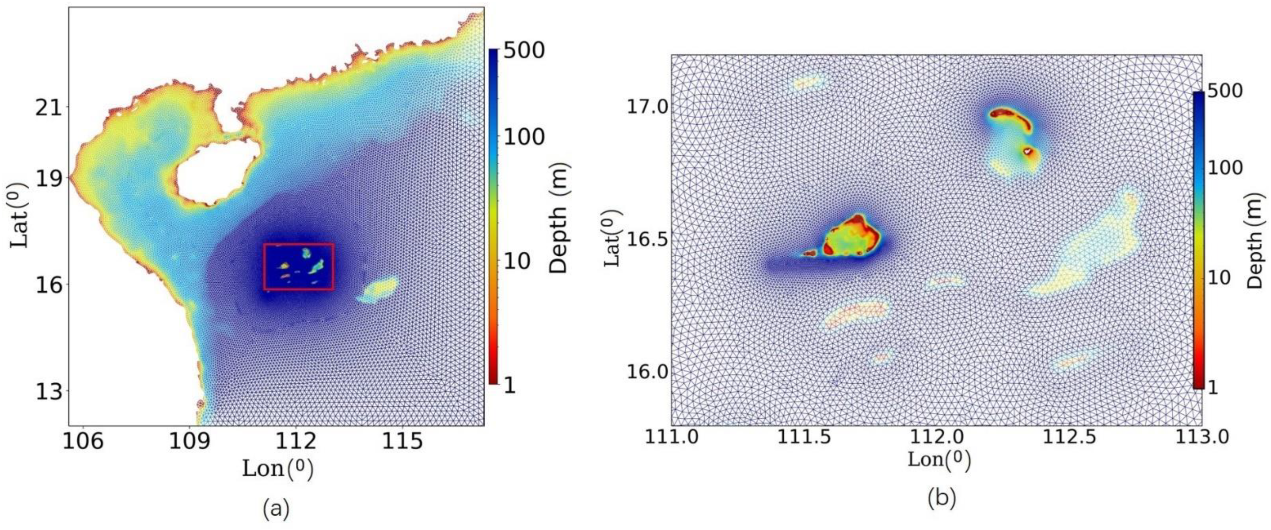
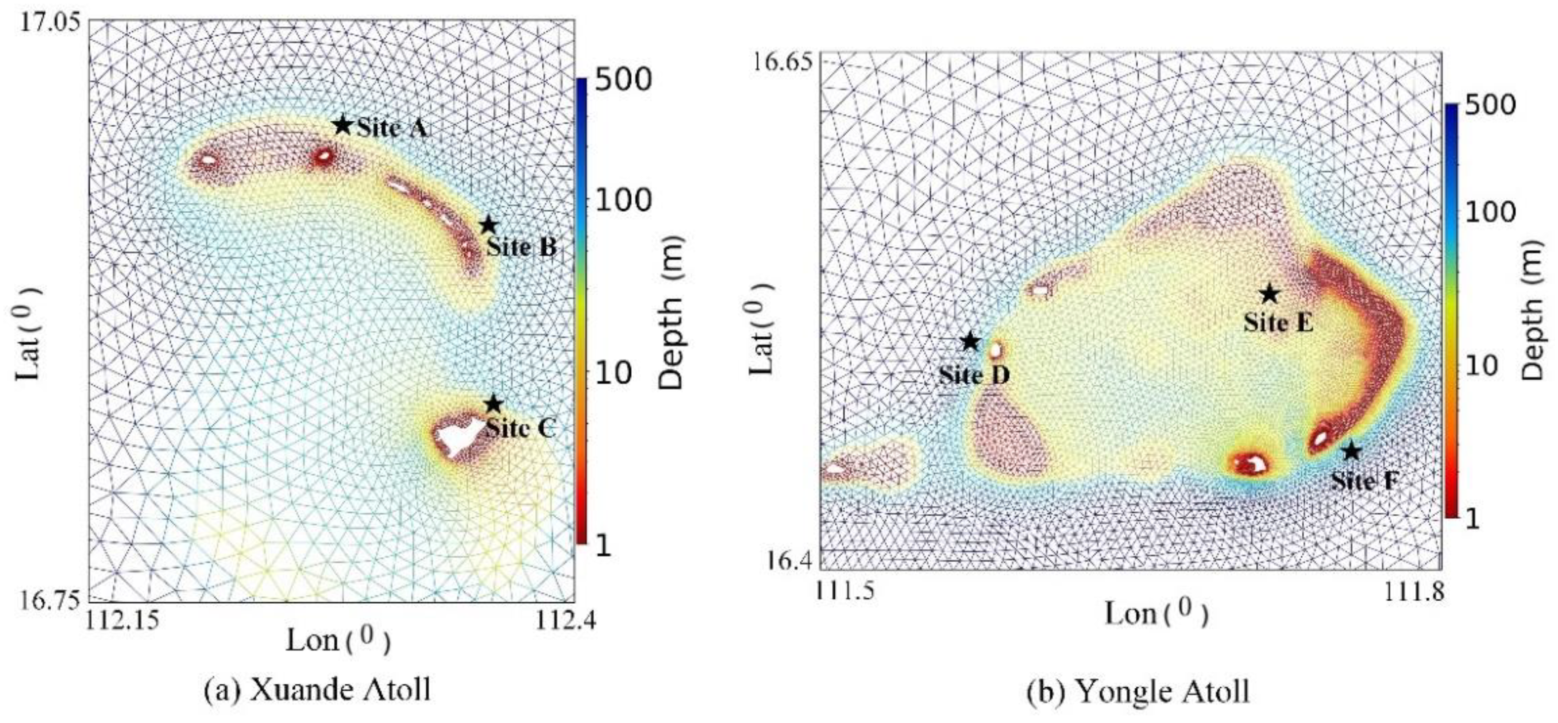
Similar to the issues encountered in the Hawaiian Islands [29], wave transition modelling from the South China Sea to the reefs and islands requires high geometric resolution in this area. As the Xisha Islands only occupy a very small area of the South China Sea, grid modelling becomes a challenge, due to the large span of spatial bathymetry. To tackle this issue, a triangular unstructured grid model was constructed in the third-generation spectral wave model WAVEWATCH-III (WW3). As shown in Figure 2, the resolution of the unstructured numerical grid varied from 3 km to 300 m, in order to distinguish the effects of the reefs and islands. The Xisha Islands are distributed over a maritime area of around 15,000 square kilometers, with a land area of approximately 7.75 square kilometers. A gird resolution of 300 m was enough to resolve the islands and reefs. The boundary condition of the WW3 model was set as an open boundary at the right side and bottom side of the domain. Bulk wind and wave parameters were outputted and archived for all the grid points spanning the Xisha Islands, comprising the data source used in this study.

2.3. Validation of Hindcast Wave Characteristics

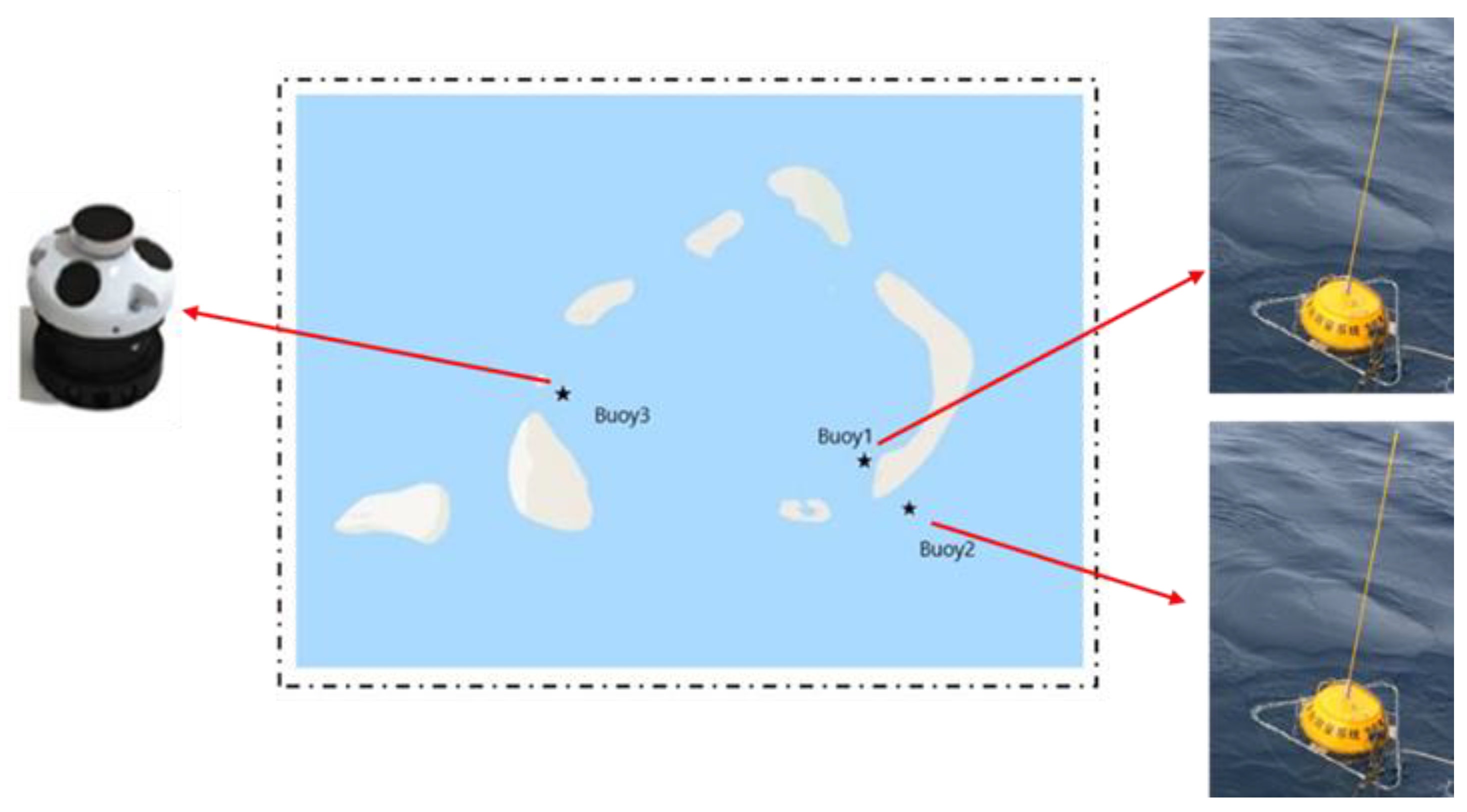
Since 2014, an observation system has been installed in a typical Crescent Group reef off the coast of the Xisha Islands. At the three locations marked with black stars in Figure 3, instrumented wave observations were carried out to capture wind-generated wave states. The measurement devices consist of two Datawell directional waverider devices (Buoy1 and Buoy2), as well as an ADCP (acoustic Doppler current profiler; Buoy3). Detailed information of our observation system can be found in [21].
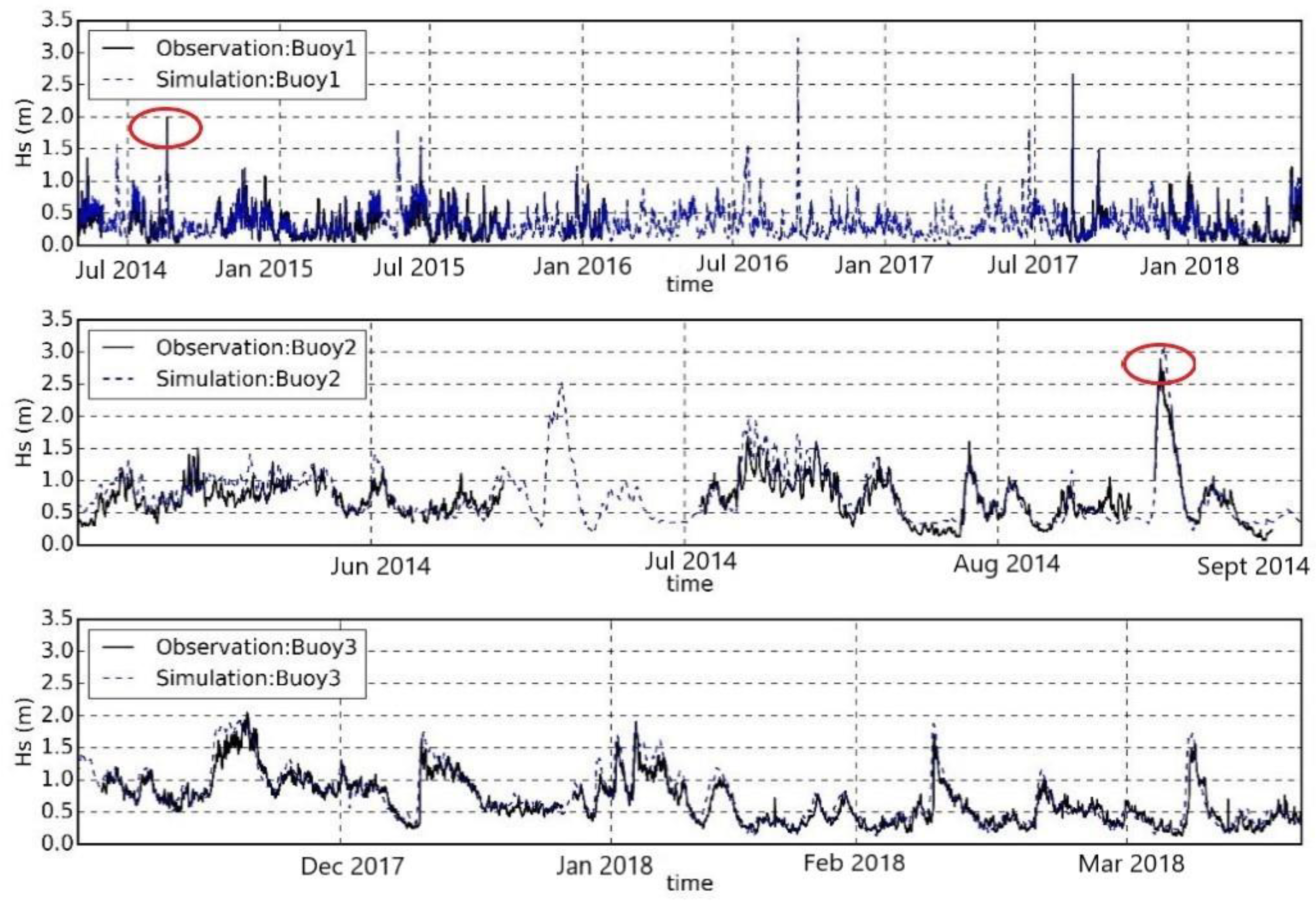
Buoy recordings were used to ensure that our hindcast data were accurate. Figure 4 shows a comparison of the time-series Hs data at three Buoy locations in different measuring periods, from which it can be seen that a high level of consistency was reached. Table 1 provides the statistical comparisons between wave WW3 hindcast data and buoy data. In general, Pearson’s correlation coefficients indicated that the model and buoy Hs were in good agreement. The Pearson’s correlation coefficients were 0.881, 0.904, 0.922. The Bias were 0.021 m, 0.076 m, and 0.025 m of Buoy1, Buoy2, and Buoy3, respectively. These results indicate that the unstructured wave forecast model can be used to accurately simulate wave propagation near islands and reefs. The computational efficiency of the unstructured numerical grid was also tested in [21].
Figure 4 shows an overall good agreement between the simulation and observation. It is also important to know the agreement in severe conditions. In Figure 5, a detailed comparison of Hs during typhoon Kalmeage waves is shown. The simulated peak Hs matches well with the observed peak Hs during the typhoon passage at both Buoy1 and Buoy2. In shallow water, the simulated peak Hs is almost the same at Buoy1. In deep water, the simulated peak Hs is 0.18 m larger than the observed peak Hs at Buoy2.

2.4. Extreme Value Analysis Methods

Extreme value theory has been widely used to estimate the regression values of meteorological and ocean data, such as wind speed, significant wave height, tide level, precipitation, and so on [26]. The extreme value analysis of time-series data can be divided into two main methods: the first involves pre-processing the data by taking the block maximum value for a sufficient period of time, such as the annual maxima value (AM). The block maximum is theoretically calculated with the Generalized Extreme Value distribution function (GEV) [30]:
G E V ( x , ξ , μ , σ ) = exp { [ 1 + ξ ( x μ σ ) ] 1 / ξ }
where μ, σ, and ξ are location, scale, and shape parameters, respectively.
The second method is to perform Peak Over Threshold processing on time-series data, using the Generalized Pareto distribution for probability-distribution fitting. The Peaks-Over-Threshold method is a sampling technique that uses exceedances above a given threshold to create a sample. The Generalized Pareto Distribution (GPD) can be used to approximate a sample of exceedances beyond a high threshold:
G P D ( x , u , σ , ξ ) = 1 ( 1 + ξ ( x u σ ) ) 1 / ξ
where σ and ξ are scale and shape parameters, respectively, and u is the threshold.
When designing marine structures, such as wave energy devices and offshore wind turbines, it is necessary to consider their survivability in extreme sea conditions. The main purpose of extreme value analysis is to estimate the probability distribution of extreme value variables based on empirical sample data, in order to calculate the extreme sea state that represents a small probability event once in n years. The environmental contour approach has been widely used in the process of designing offshore structures, as well as in standards and guidelines such as the DNVGL-RP-C205 [31]. The idea is to define contours in the sea-state space (usually Hs, Tz), along which extreme responses with a given return period should occur [32]. This method finds the most likely design point of structural failure on the environmental contour line of a specific return period, which is input as a design parameter to obtain the same return period structural response, allowing us to avoid long-term response forecasting [27]. The process of developing an environmental contour typically involves statistical modelling of the joint probability density function of the variables of interest, then constructing a contour based on that joint distribution [33,34]. In the first step, the marginal distribution of Hs is typically modeled with the two-parameter Weibull distribution:
F ( H s ) = 1 exp [ ( H s / α ) β ]
The exponentiated Weibull distribution is a novel distribution choice for sea-state models. It extends the two-parameter Weibull distribution with a second shape parameter, δ , used as an exponent of the cumulative distribution function (CDF):
F ( H s ) = ( 1 exp [ ( H s / α ) β ] ) δ
for Hs > 0; here, β > 0 is the first shape parameter, δ > 0 is the second shape parameter, and α > 0 is the scale parameter of the distribution. In the case δ = 1, the exponentiated Weibull distribution becomes the two-parameter Weibull distribution. The zero up-crossing period follows a conditional log-normal distribution. For the second step, the inverse first-order reliability method (IFORM) [32] was used for the construction of the contour.

3. Wind and Wave Climate Analysis

3.1. Spatio-Temporal Variations of Wind Characteristics

The wind speed and wind direction change with time and height above sea level. The standard reference height is 10 m above the sea surface. The common practice in ocean engineering is to give the average duration of wind speed and reference elevation, combining them with local wind-related parameters such as the wind-profile function, gust coefficient, and autocorrelation wind spectrum, in order to describe wind conditions at different temporal and spatial scales reasonably [29].
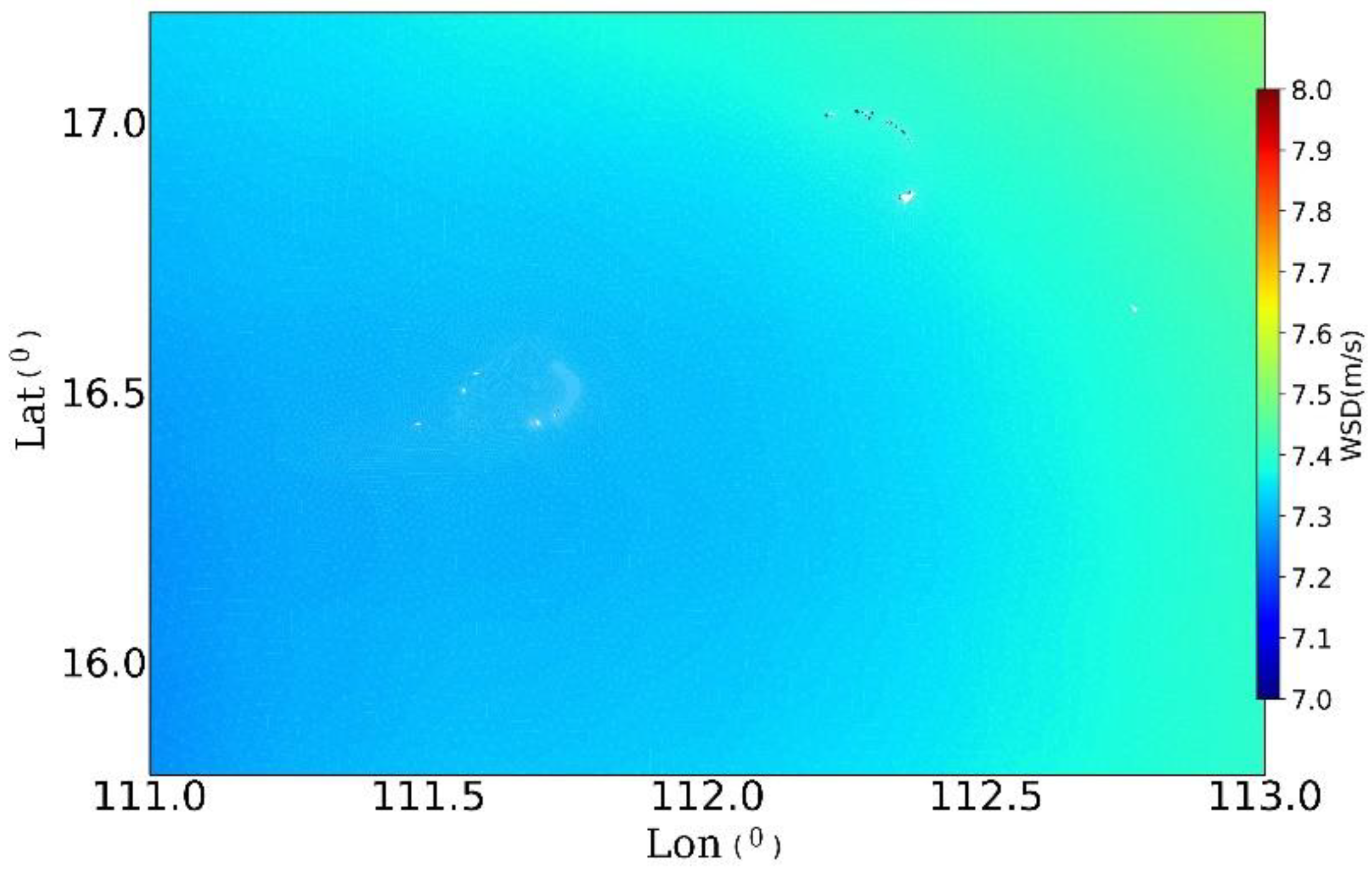
Figure 6 shows the spatial distribution characteristics of the hourly averaged wind speed (WSD) covering the Xisha Islands. Note that, direction in this paper is defined as those directions where the wind and waves come from. In general, the wind field did not change significantly in such a small spatial scale over the Xisha Islands.
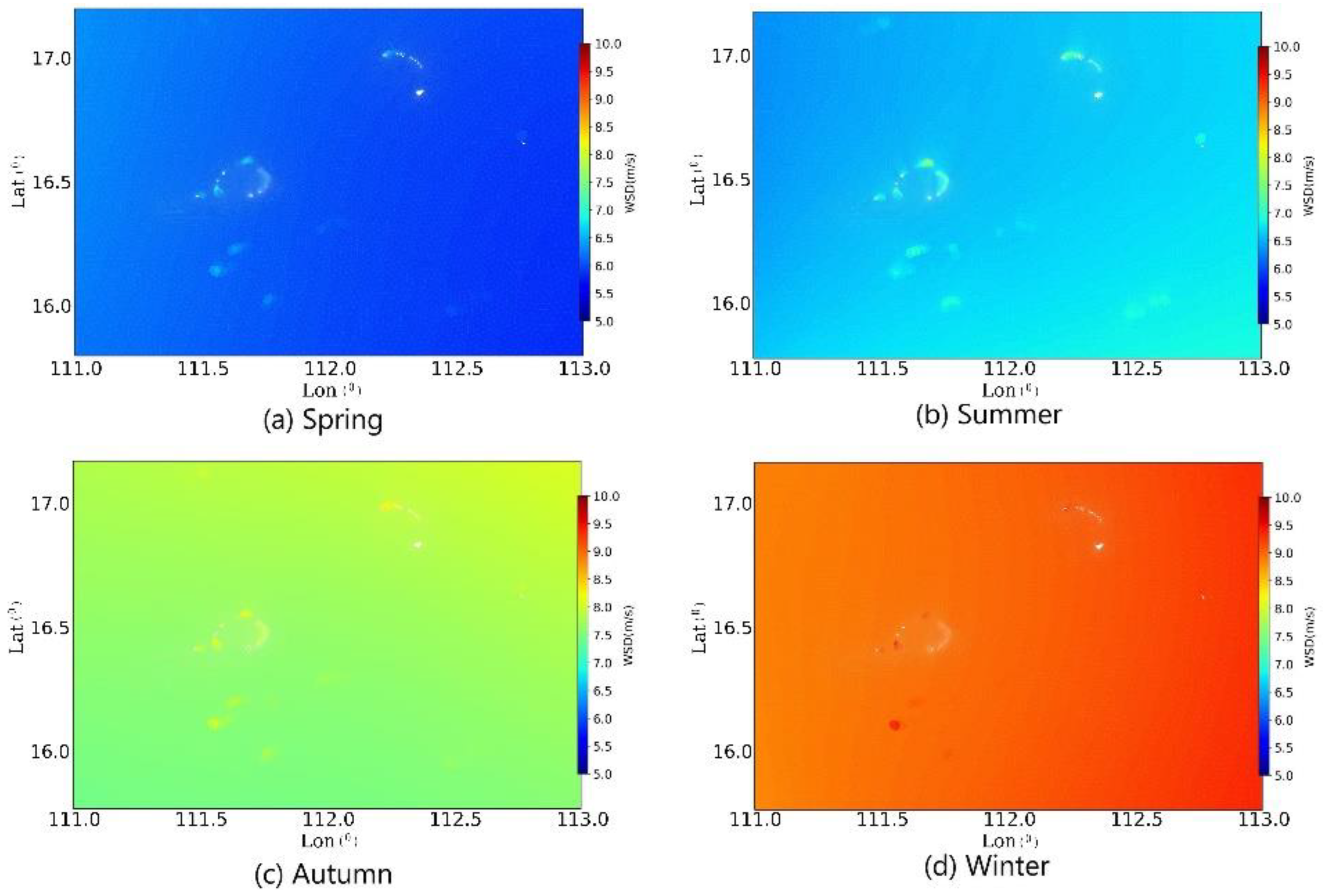
Figure 7 shows the spatial distribution of the seasonal mean WSD at the Xisha Islands. The mean WSD in winter was the highest, exceeding 8.5 m/s in most sea areas of the Xisha Islands; meanwhile, the mean WSD in spring was the lowest, ranging from 5–6.5 m/s. In summer, the mean WSD was higher in the southeast of the Xisha Islands. In autumn and winter, the mean WSD was higher in the northeast of the Xisha Islands.

3.2. Spatio-Temporal Variations of Wave Characteristics

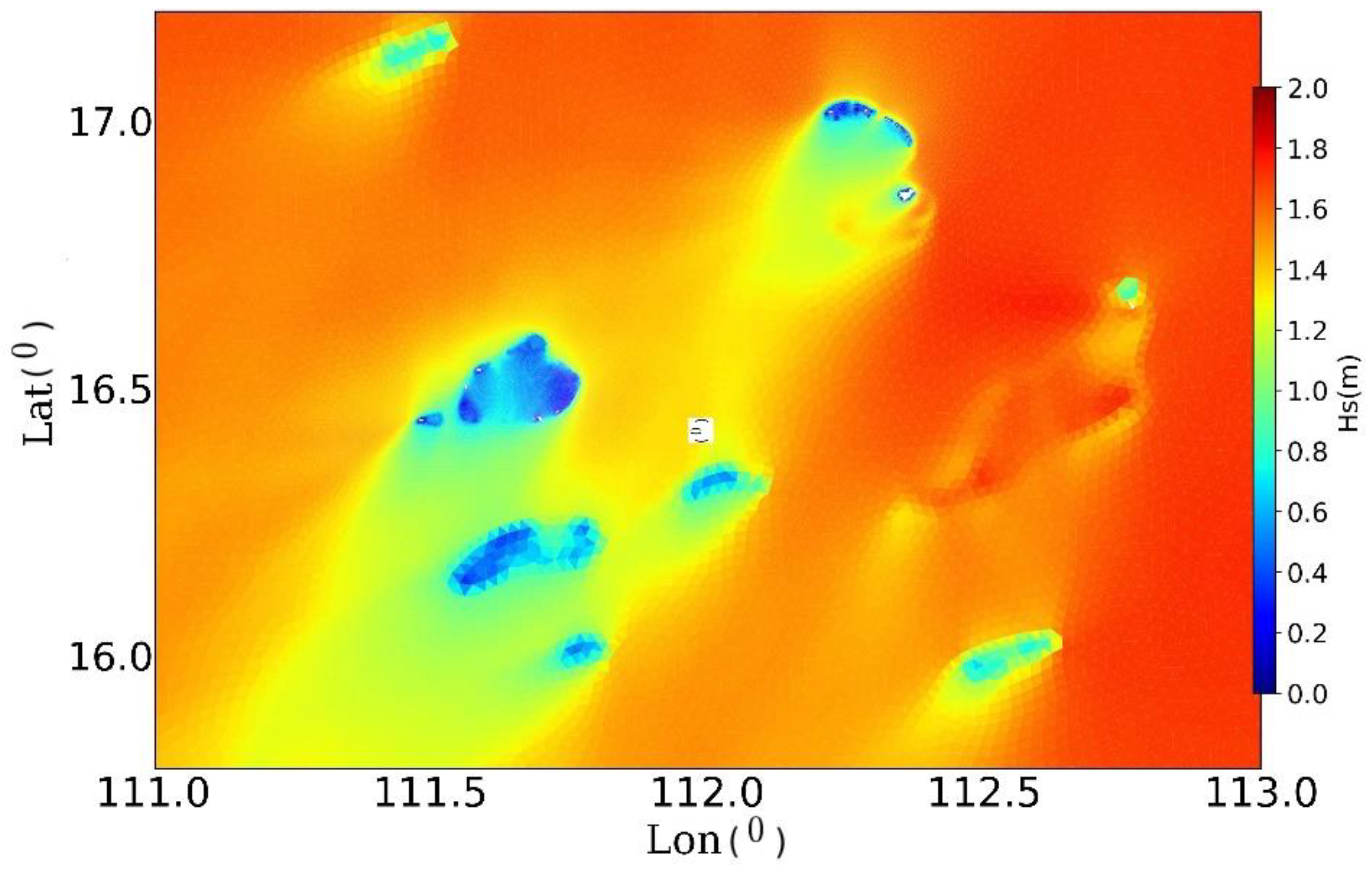
Wave conditions are critical for the design and deployment of marine structures such as wave energy converters and floating wind turbines. Through the bulk wave parameters output by WW3, the mean values of the significant wave height (Hs) at each grid point were calculated. Figure 8 shows the distribution of the mean Hs over the Xisha Islands. Due to the variations in reef topography, the mean Hs in the Xisha Islands was unevenly distributed. In the deep-water area of the Xisha Islands, the mean Hs ranged between 1.5–1.8 m, while it decreased rapidly when approaching the islands and reefs: the mean Hs inside the atoll was only 0.2–0.4 m. The overall wave conditions of the Xuande Atoll were worse than those of the Yongle Atoll.
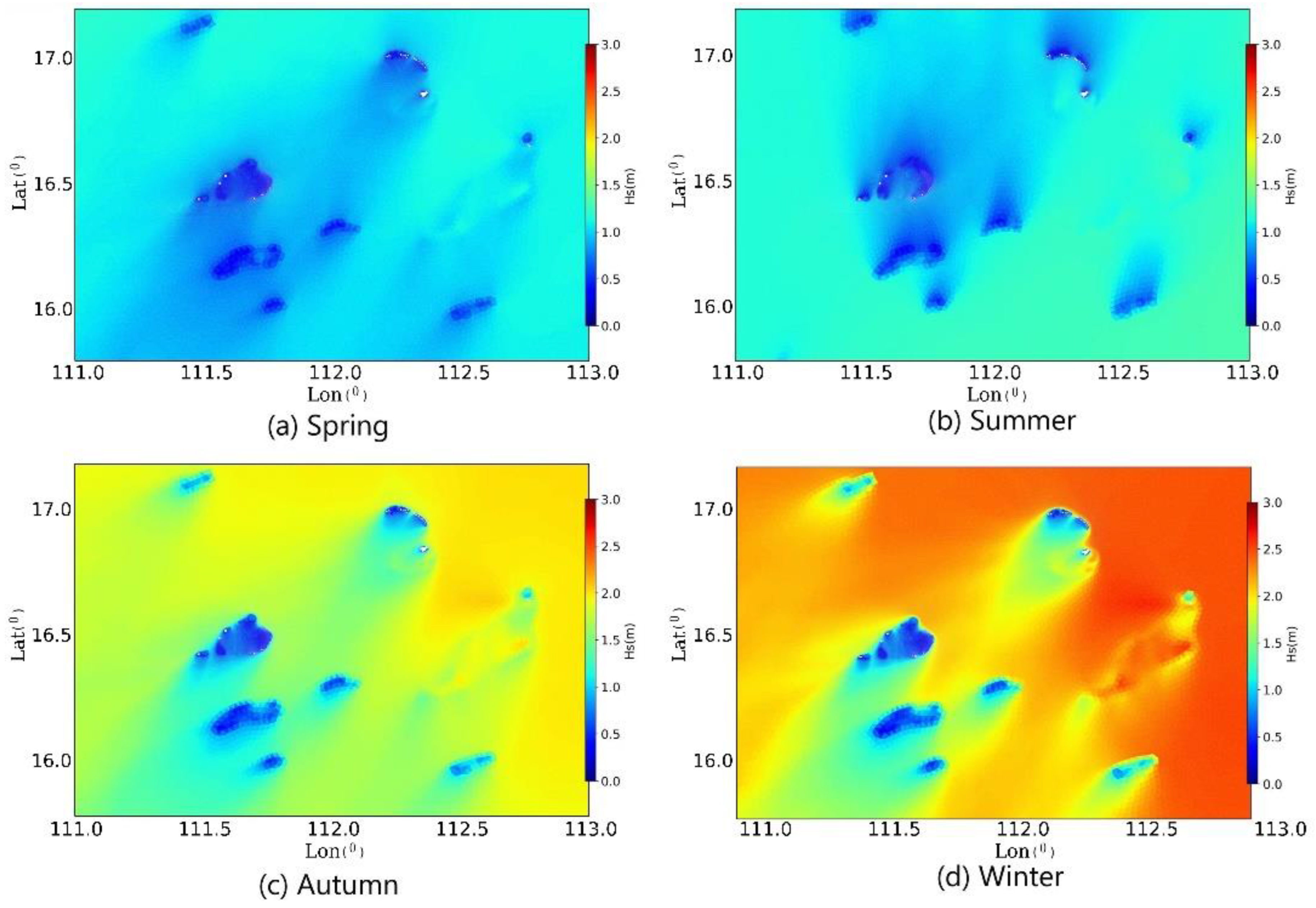
The seasonal mean Hs distributions are shown in Figure 9. In spring, the mean Hs in the open sea ranged between 1.0–1.3 m. In summer, the mean Hs in the open sea ranged between 1.2–1.5 m. In autumn, the mean Hs in the open sea ranged from 1.5–2.2 m. Finally, in winter, the mean Hs in the open sea ranged between 2.2–3 m.
From the components of the wave frequency spectrum, waves can be divided into wind waves, swell waves, and mixed waves. In the calculation process of WAVEWATCH-III, the wind wave and swell parts can be separated by their dynamic frequency, based on the wave age. This numerical method of spectral separation further divides the wave spectrum into wind wave components and swell components. Then, the wind wave ratio coefficient, representing the contribution of the wind wave component to the total wave energy, can be derived.
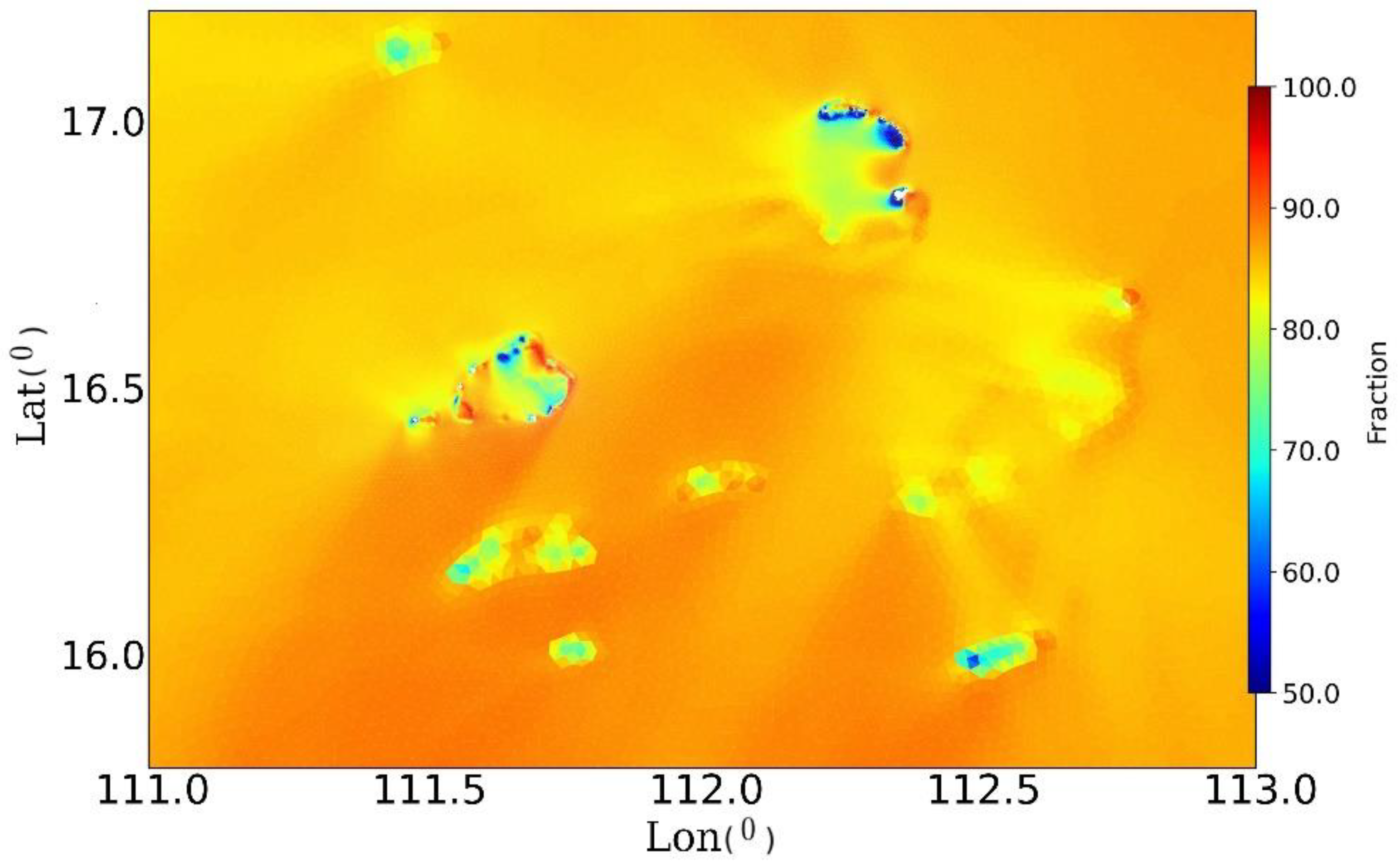
Figure 10 shows the distribution of the average annual wind wave ratio coefficient in the Xisha sea area. In the open sea, wind wave components were dominant, with most of the sea area ratio coefficients being above 85%; in the sheltered sea areas affected by islands and reefs, the wind wave components were reduced, and the impact of swells on these areas was relatively large. An exemplary area is the southwest side of the Xuande Atoll, where the wind wave component in this area only accounts for 50–60%.

3.3. Long-Term Wind Characteristics

The 10-m wind speed and direction data at a random location were extracted from the hindcast wind field data to represent the wind characteristics in the Xisha Islands. The observation period was from 1988 to 2019, updated once every three hours. Table 2 shows the wind speed classification results according to the Beaufort wind force scale. From the table, it can be seen that the main wind speed frequency was concentrated from Class 3 to Class 6, accounting for 64.11%. The frequency of strong winds above Class 6 was 4.08%, mainly in November and December. The maximum wind speed at the site was 40.57 m/s, which occurred in September. The highest mean wind speed was in December, reaching 10.49 m/s. The lowest wind speed standard deviation was observed in March, while the largest standard deviation was in November.
Figure 11 shows a rose plot of the wind speed and direction at the Xisha Islands throughout the entire hindcast period. The dominant wind direction in the rose plot appeared in the N-E and S directions. The wind speed distribution in the N-E direction was wide, while the wind speed distribution in the S direction was relatively concentrated and small.
Figure 12 shows the rose plots of wind speed and wind direction divided by month. From March to April, the wind direction was relatively scattered and distributed in N-E to S directions; meanwhile, from May to August, the wind direction was concentrated in the S direction. September was a transitional month. From October to February of the following year, the wind direction was stable and concentrated in the N-E direction.

3.4. Long-Term Wave Characteristics

As the Xisha Islands consist of a large number of islands and reefs, the wave conditions may significantly differ from island to island. The high-resolution wave data calculated by the unstructured WW3 model allowed us to calculate long-term wave statistics and conduct analysis on specific islands and reefs. As shown in Figure 13, six sites were selected near important islands with busy human activities. These sites include Island A, Island B, and Island C in the Xuande Atoll, as well as Island D, Island E, and Island F in the Yongle Atoll. Among these characteristic sites, Island E is located inside the lagoon, with a water depth of 30 m. The other sites are distributed in the open sea, near islands and reefs. The water depth at these sites ranges between 40 m and 60 m. The summary information of these sites is provided in Table 3.
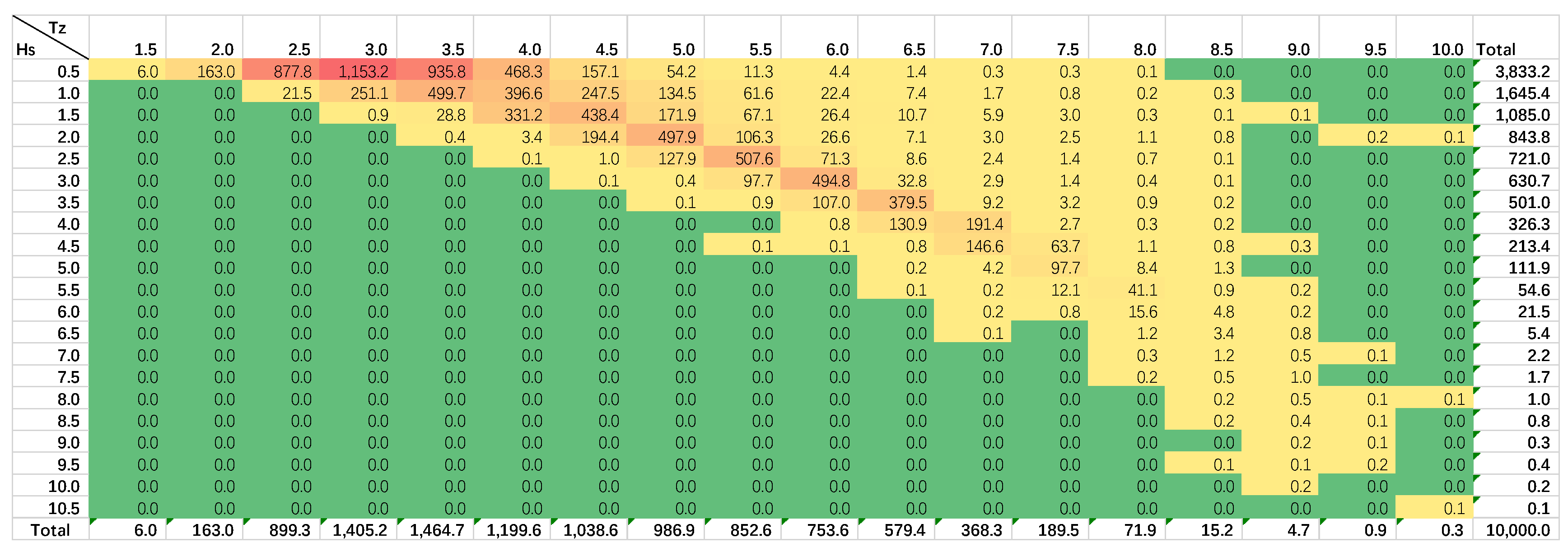
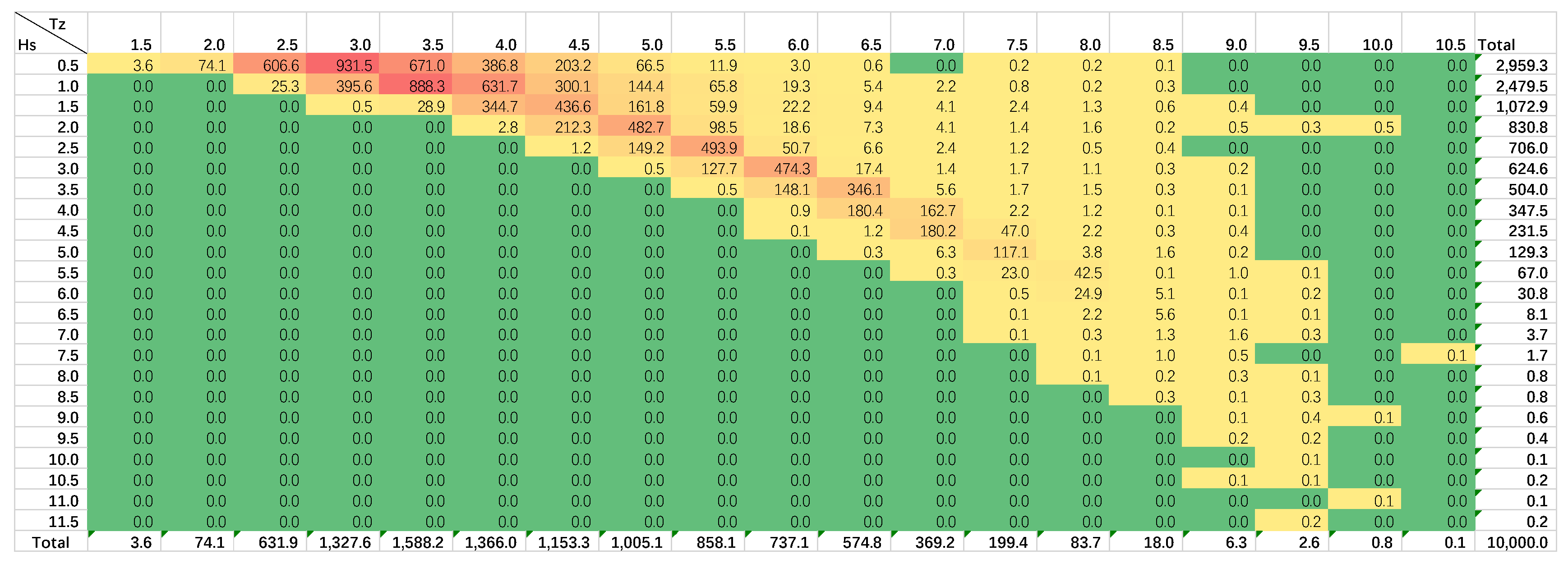
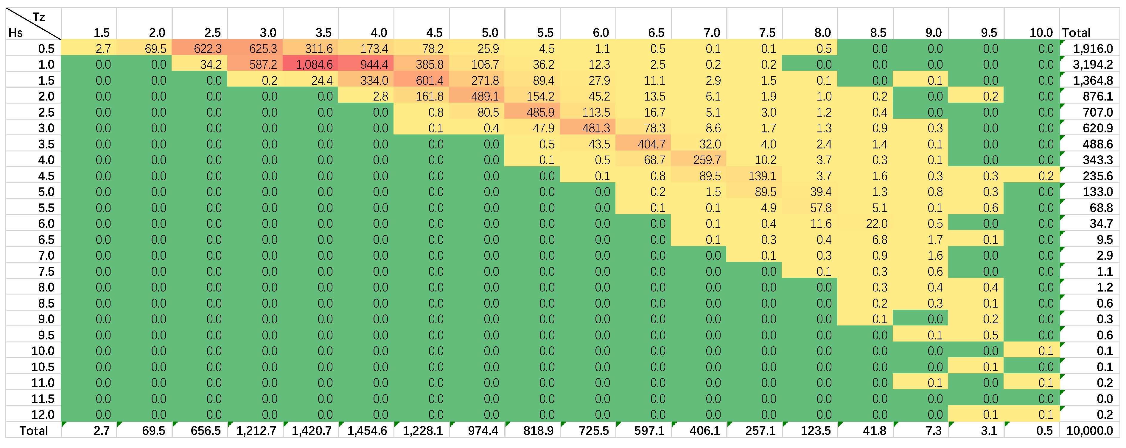
The long-term distribution of wave conditions can be represented by a scatter diagram of sea-state parameters. The scatter diagram reflects the historical occurrence frequency of a given sea state. In this paper, Hs and Tz (zero up-crossing period) are used for the description of the sea state. Figure 14, Figure 15, Figure 16, Figure 17, Figure 18 and Figure 19 show the respective wave scatter diagrams at the reference sites. The wave conditions at Islands A, B, and C of the Xuande Atoll were similar, while the wave conditions at Islands D, E, and F of the Yongle Atoll differed. These results can be used as a reference condition for the fatigue analysis of offshore engineering structures.
Figure 20 shows rose plots of the Hs and mean wave direction for the characteristic sites. It can be seen that the main wave directions at the three characteristic sites of the Xuande Atoll were all in the N-E direction, while Island A and Island B were also under the influence of waves from the SSE direction. The directional distributions of waves near the different sites of the Yongle Atoll were quite different. The main wave direction at the Island D site was the N-E direction. Meanwhile, as Island E is inside the Yongle Atoll lagoon, there was no obvious main wave direction. The wave directions with a higher frequency at Island E were NNW and S. Island F was dominated by the waves from the E direction.

4. Extreme Wind and Wave Analysis

4.1. Extreme Value Analysis on Wind Speed

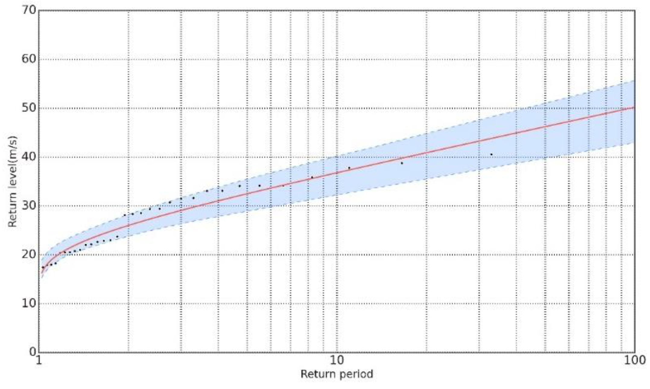
The AM-GEV method was used for the wind speed extreme-value analysis. The first step was to select the maximum wind speeds appearing in the 32-year wind speed time history data as a sample, and then perform empirical function fitting. Figure 21 shows the relationship between the calculated wind speed regression period and the regression value. The 100-year wind speed calculated by the AM-GEV method was 50.22 m/s. A 95% confidence interval for the wind speed was obtained as [42.94 m/s, 55.68 m/s].
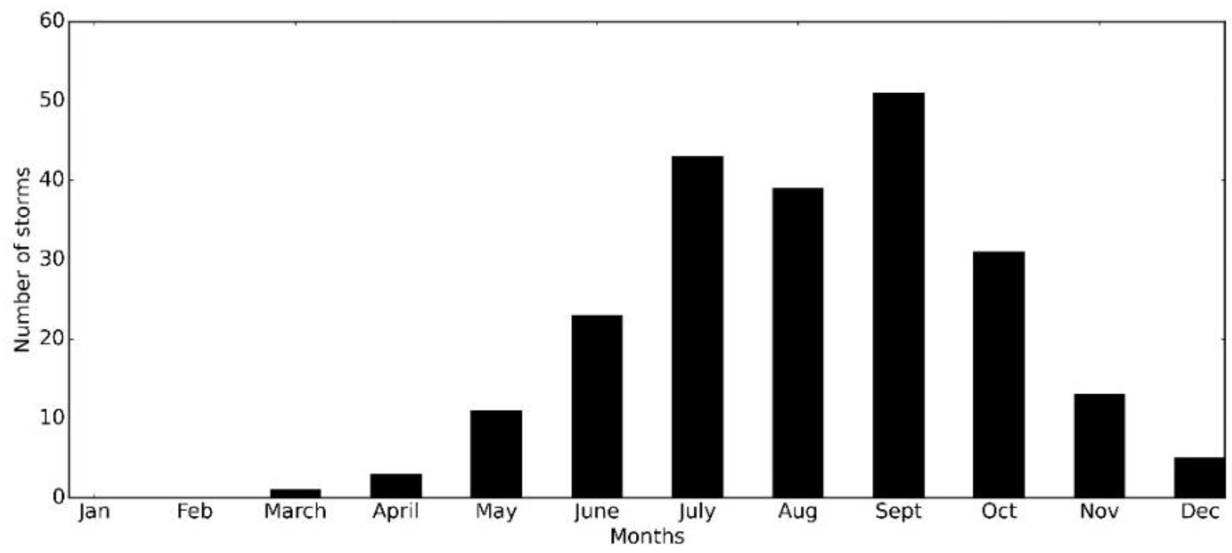
To perform the peak over threshold method, the storm process affecting the Xisha Islands was first determined. The storm period was extracted from the best track data of the Joint Typhoon Warning Center. The total number of storms was found to be 220.
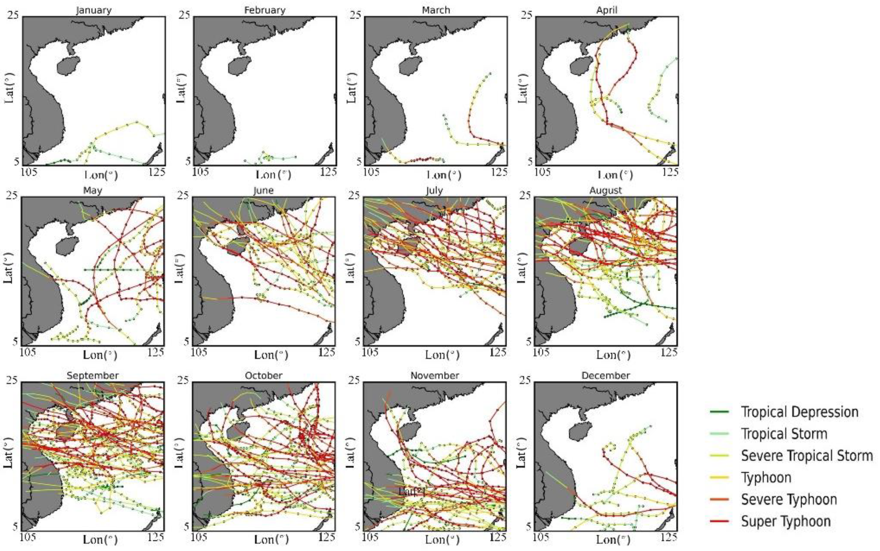
Figure 22 shows the paths of all tropical storms affecting the Xisha Islands from 1988 to 2019, classified by months, while Figure 23 shows the monthly distribution of tropical storm numbers. The number of tropical storms had obvious seasonal characteristics. The typhoon season started from April, and the number of storms gradually increased. The frequency and intensity of typhoons reached a peak value in September. From December to March of the next year, almost no tropical storms occurred. From the general perspective of the storm path, most tropical storms entered the South China Sea from the Northwest Pacific Ocean. Summer tropical storms tend to land on the coast of China, while winter storms tend to land on the coast of Vietnam. Taking the position of the Xisha Islands as a reference position, most of the typhoon tracks were spread from the northwest to the southeast of the Xisha Islands.
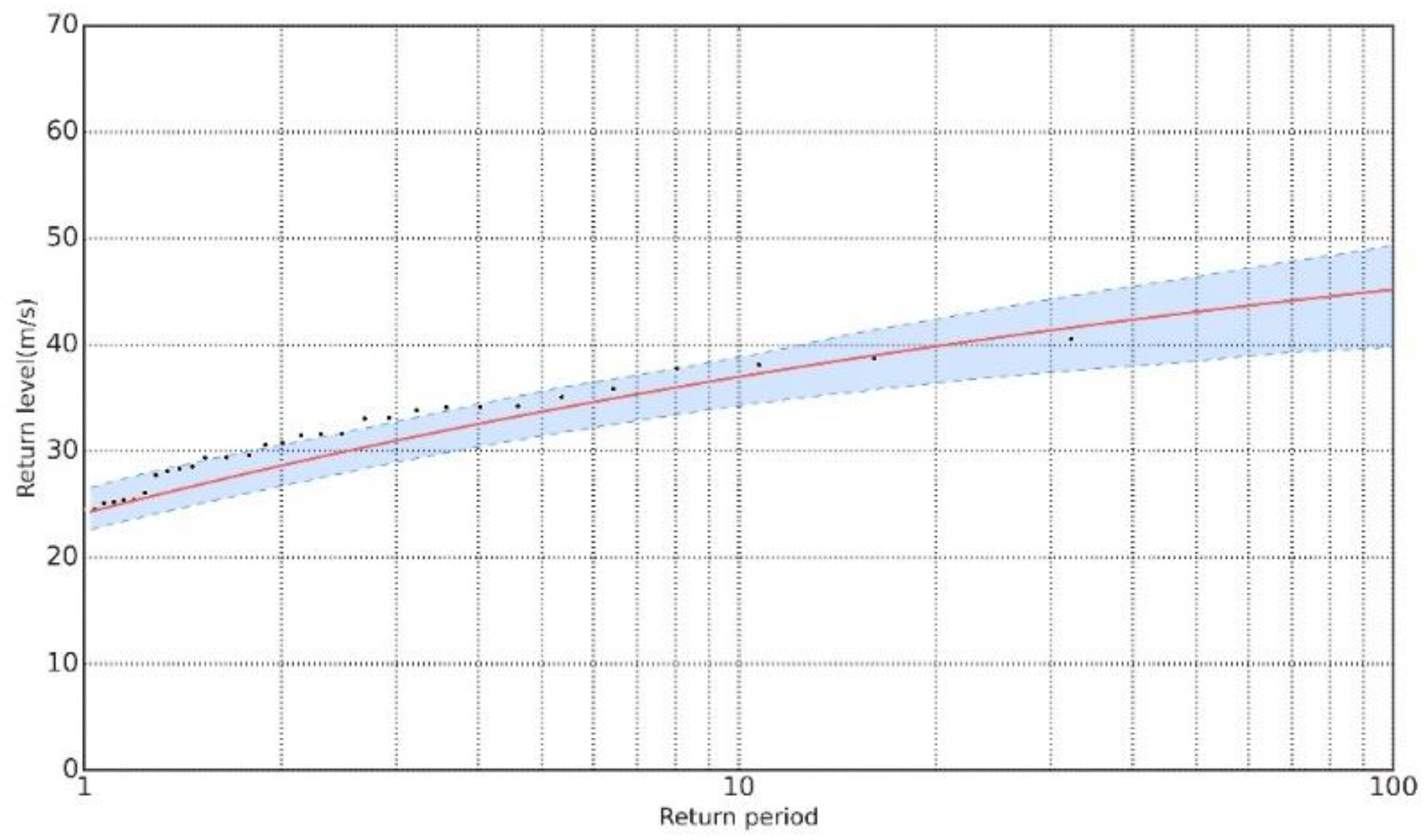
Once the start and end times of the storms were determined, the maximum wind speed during the 220 storms could be extracted from the time history data, which can be used as an independent sample of storm extreme values. Of the 220 storm maxima samples, some of them had a limited impact on the Xisha Islands. Therefore, a threshold was used to remove these samples. According to the recommendation in [27], we used 1.5 times the average wind speed as the threshold. Figure 24 shows the regression curve of the GPD using the Peaks-Over-Storm threshold. The calculated wind speed of the 100-year return value was 45.19 m/s. A 95% confidence interval for the wind speed was obtained as [39.77 m/s, 49.36 m/s].

4.2. Extreme Value Analysis on Significant Wave Height

Considering that the length of our simulation wave data is 32 years long, the block period is chosen as a year. The estimation of the GEV and GPD model parameters are based on the maximum likelihood estimator. The return level plots using the AM-GEV method are shown in Figure 25. Of all the sites, Island A had the largest storm Hs larger than 10 m during the last five years. The GEV distribution was reasonably well-fitted except for Site F.
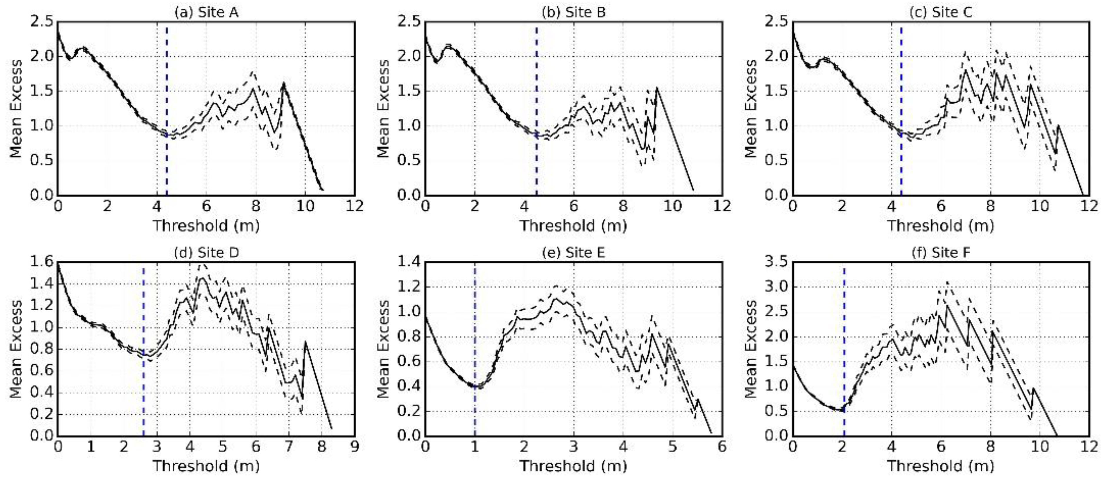
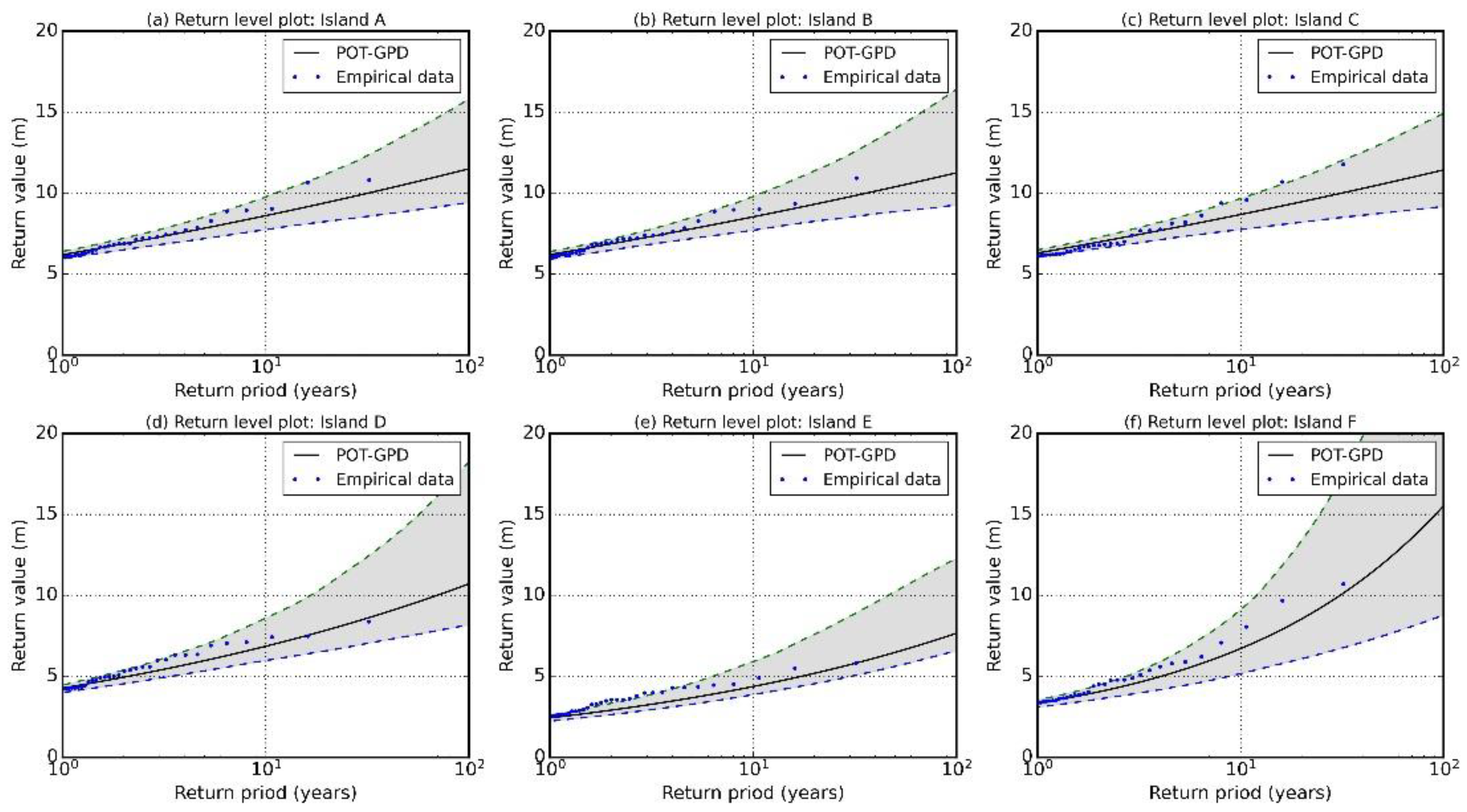
To solve a critical problem in the POT-GPD method, an appropriate threshold needs to be selected. Different thresholds will lead to a large variety of return level estimates. Following [21], threshold selection was done on the basis of the evaluation of the mean residual life (MRL) trend in the function of a defined threshold range. More precisely, the threshold should be chosen as the point in whose proximity the trend changes from approximately linear to unstable. The mean residual life plots at six sites are shown in Figure 26, with thresholds at 4.3 m, 4.5 m, 4.4 m, 2.6 m, 1.0 m, and 2.1 m, respectively. The return level estimation results using the POT-GPD method are shown in Figure 27. After proper threshold selection, the POT data can be well fitted by the GPD model.
The summary and comparison of the 100-year return levels estimated by the GEV approach and POT-GPD approach are summarized and listed in Table 4. The confidence intervals legitimize the differences among the different approaches. The best fitted results of the two approaches were basically similar at Site D and Site E. The POT-GPD method tended to underestimate the return levels at Site A, Site B, and Site C, while the GEV method tended to underestimate the return levels at Site F.

4.3. Extreme Sea-State Estimation at Selected Sites

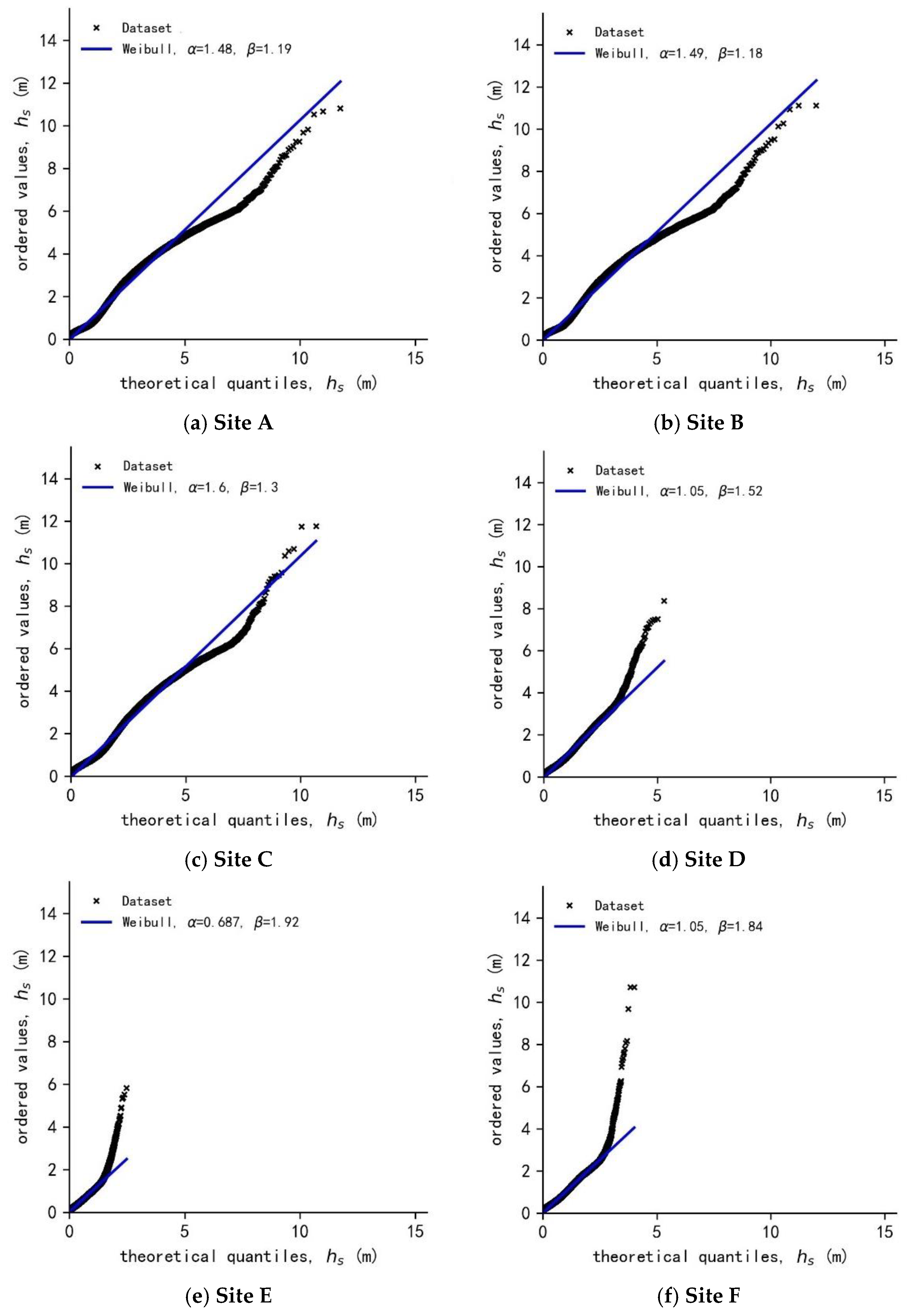
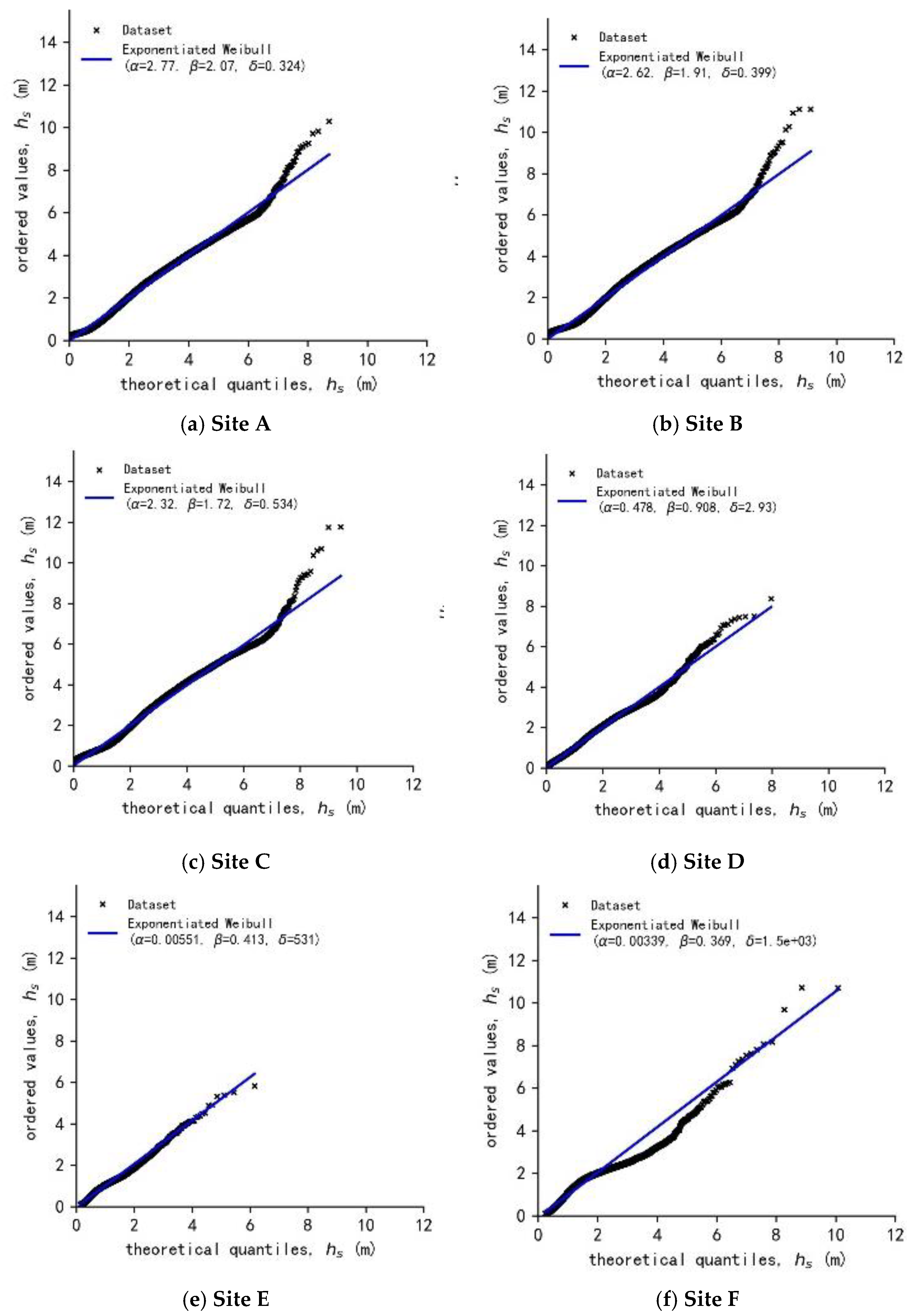
Figure 28 and Figure 29 show the fitting results of significant wave heights using the two-parameter Weibull distribution and the exponentiated Weibull distribution, respectively, at different sites. In Figure 28, the QQ-plots show that the Weibull distributions provide good model fit at Islands A, B, and C. The fitting parameters for these sites were similar. However, the Weibull distributions predicted too low wave heights at high quantiles for Islands D, E, and F. In Figure 29, the results are the complete opposite. The QQ-plots show that the exponentiated Weibull distributions provided a fairly good fit at Islands D, E, and F, while predicting too low wave heights at high quantiles for Island A, B, and C.
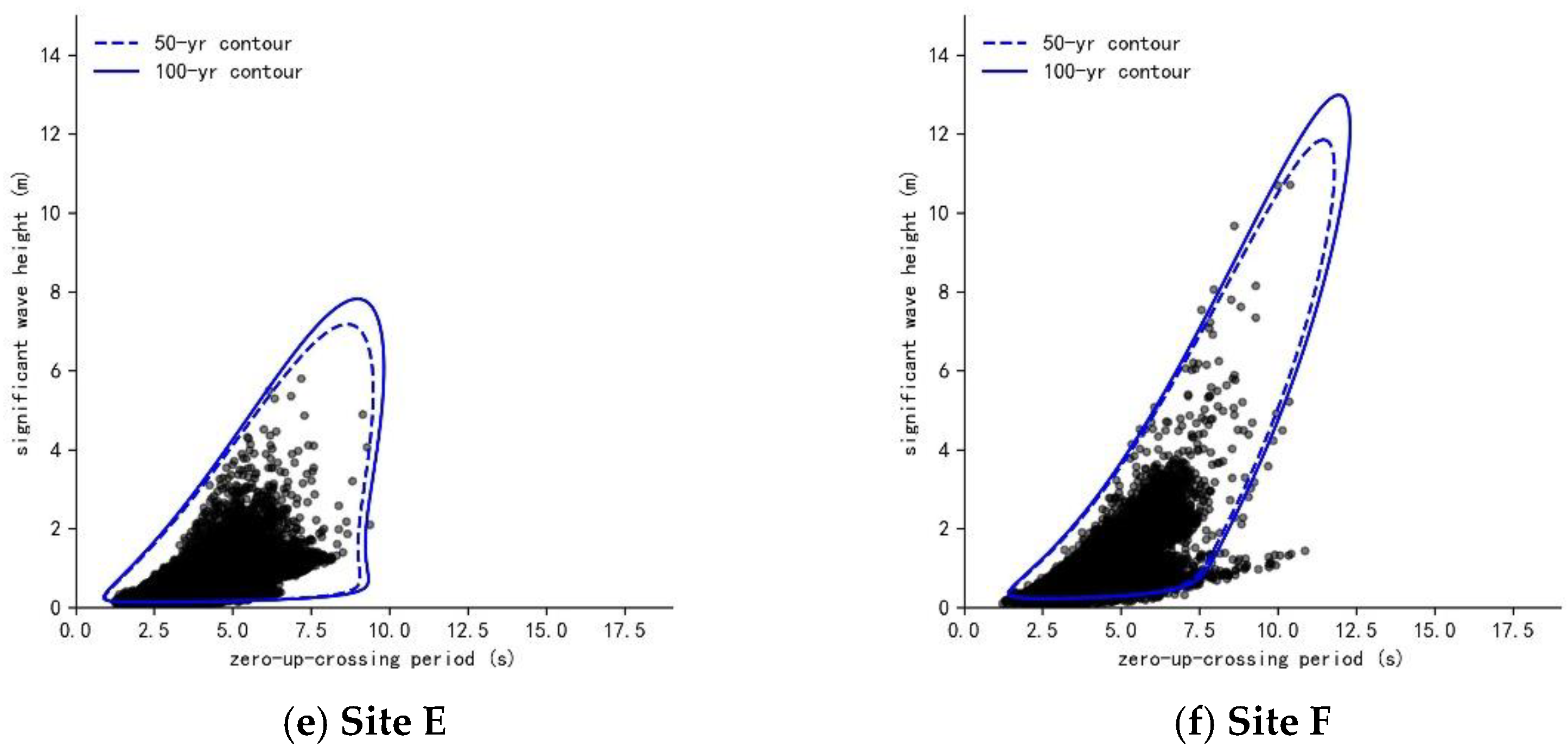
The fitting parameters are listed in Table 5. It should be noted that the sea states at Site E and Site F are much calmer than the other sites at normal times due to the sheltering effect of the surrounding reefs. The significant wave heights at Site E and Site F are relatively smaller and compact. As a result, the value of the scale parameter α estimated using the exponentiated Weibull distribution is relatively small compared with the other sites. Generally, it can be concluded that the Hs data of the three sites in the open sea at the Xuande Atoll fit well with the two-parameter Weibull distribution, while the exponentiated Weibull distribution fitting results were better for the sites at the Yongle Atoll, which is sheltered by reefs and islands. After determining the well-fitted distributions, the corresponding contour plots of the sea-state parameters were calculated and are shown in Figure 30.
After the environmental contour method was estimated, the maximum Hs on the contour line was selected. The single-value extreme value analysis results were compared with the environmental contour results in Table 6. Generally, the 100-year return level Hs estimated using the Environmental Contour method was close to the GEV results. An advantage of the Environmental Contour method was that it could avoid the unrealistically large values that could appear in the extreme-value analysis results.

5. Conclusions

The wind and wave environmental conditions in the Xisha Islands of the South China Sea were described qualitatively and quantitatively in this research. First and foremost, the numerically modeled long-term wind and wave data employed in this study were thoroughly explained and validated. The wind data had a spatial resolution of 0.1° and covered the whole South China Sea. The resolution of unstructured wave hindcast data varied from 3 km to 300 m, enabling the examination of near-island sites in the South China Sea at the Xisha Islands.
First, the spatial wind and the wave environment were analyzed. In general, the mean wind speed ranged between 7–8 m/s, with little spatial variation. The spatio-temporal variations in the wave characteristics for the Xisha Islands were determined in terms of annual mean Hs, seasonal mean Hs, and annual mean wind wave ratio coefficient. The impact of swell components was more evident in the sheltered areas, affected by islands and reefs.
Then, the frequency and directional distribution of wind and wave characteristics at various sites were analyzed. The main wind speed frequency throughout the year was concentrated from Class 3 to Class 6, accounting for 64.11%. The dominant wind directions in the rose plot appeared in the N-E and S directions. Six sites near the main islands were analyzed in order to provide detailed and structured insights into the wave conditions of the Xisha Islands. The scatter diagrams and rose plots at these sites facilitated the quantitative description of the sea-state conditions in normal times.
In the extreme wind and wave analysis section, the extreme wind speed was first evaluated, with respect to a 100-year return period, using the AM-GEV method and the POT-GPD method. The 100-year wind speed calculated using the AM-GEV method was 50.22 m/s, while the wind speed calculated with a 100-year return value using the POT-GPD method was 45.19 m/s. The best track data from the Joint Typhoon Warning Center were also used to study tropical storm events. There were 220 tropical storms over the last 32 years in the study area, where most tropical storms made their way into the South China Sea from the Pacific Northwest. Summer tropical storms tend to hit the Chinese coast, whereas winter storms are more likely to hit the Vietnamese coast.
Finally, the extreme wave environment was analyzed. The extreme Hs was evaluated at six sites using the traditional AM-GEV method and the POT-GPD method. It was found that these two approaches have different performances at different sites. Despite the similar results at Site D and Site E, the POT-GPD method tended to underestimate the return levels at Site A, Site B and Site C, while the GEV method tended to underestimate the return levels at Site F.
Extreme wave environmental contours were then established for multi-variable extreme analysis at the six considered sites. Joint probability distributions for significant wave heights and mean wave periods were developed. It was found that the Hs data of the three sites in the open sea fit well with the two-parameter Weibull distribution, while the exponentiated Weibull distribution fitting results were better for sites sheltered by reefs and islands. Accordingly, generally, the 100-year return level Hs estimated using the Environmental Contour method was close to the GEV results. An advantage of the environmental contour method was that it could avoid the unrealistically large values that could appear in extreme value analysis results.
This research can aid in gaining a better understanding of the wind and wave climate in the Xisha Islands, which can then be used for the design, operation planning, and maintenance of marine-related engineering objects.

Author Contributions

Writing—review and editing, Z.S.; visualization, M.B.; supervision, J.D.; project administration, J.L.; formal analysis, H.Z.; funding acquisition, D.X. All authors have read and agreed to the published version of the manuscript.

Funding

This research was funded by the Ministry of Industry and Information Technology (Grant No. [2016]22, [2019]357), the National Key Research and Development Program of China (Grant No. 2017YFB0202701) and the Jiangsu Province Science Foundation for Youths (Grant No. BK20190151).

Institutional Review Board Statement

Not applicable.

Informed Consent Statement

Not applicable.

Data Availability Statement

Not applicable.

Acknowledgments

Shanhong Gao is acknowledged for providing access to the wind data sets.

Conflicts of Interest

The authors declare no conflict of interest. The funders had no role in the design of the study; in the collection, analyses, or interpretation of data; in the writing of the manuscript; or in the decision to publish the results.

References

  1. Jonathan, P.; Ewans, K. Statistical modelling of extreme ocean environments for marine design: A review. Ocean Eng. 2013, 62, 91–109. [Google Scholar] [CrossRef]
  2. Shao, Z.; Liang, B.; Li, H.; Lee, D. Study of sampling methods for assessment of extreme significant wave heights in the South China Sea. Ocean Eng. 2018, 168, 173–184. [Google Scholar] [CrossRef]
  3. Chen, X.; Wang, K.; Zhang, Z.; Zeng, Y.; Zhang, Y.; O’Driscoll, K. An assessment of wind and wave climate as potential sources of renewable energy in the nearshore Shenzhen coastal zone of the South China Sea. Energy 2017, 134, 789–801. [Google Scholar] [CrossRef] [Green Version]
  4. Wang, Z.; Li, S.; Dong, S.; Wu, K.; Yu, H.; Wang, L.; Li, W. Extreme wave climate variability in South China Sea. Int. J. Appl. Earth Obs. 2018, 73, 586–594. [Google Scholar] [CrossRef]
  5. Wang, Z.; Duan, C.; Dong, S. Long-term wind and wave energy resource assessment in the South China sea based on 30-year hindcast data. Ocean Eng. 2018, 163, 58–75. [Google Scholar] [CrossRef]
  6. Zheng, C.; Li, C. Variation of the wave energy and significant wave height in the China Sea and adjacent waters. Renew. Sustain. Energy Rev. 2015, 43, 381–387. [Google Scholar] [CrossRef]
  7. Shao, Z.; Liang, B.; Li, H.; Li, P.; Lee, D. Extreme significant wave height of tropical cyclone waves in the South China Sea. Nat. Hazards Earth Syst. Sci. 2019, 19, 2067–2077. [Google Scholar] [CrossRef] [Green Version]
  8. Shamji, V.R.; Aboobacker, V.M.; Vineesh, T.C. Extreme value analysis of wave climate around Farasan Islands, southern Red Sea. Ocean Eng. 2020, 207, 107395. [Google Scholar] [CrossRef]
  9. Cieślikiewicz, W.; Paplińska-Swerpel, B. A 44-year hindcast of wind wave fields over the Baltic Sea. Coast. Eng. 2008, 55, 894–905. [Google Scholar] [CrossRef]
  10. Rusu, L. The wave and wind power potential in the western Black Sea. Renew. Energy 2019, 139, 1146–1158. [Google Scholar] [CrossRef]
  11. Bernardino, M.; Rusu, L.; Guedes Soares, C. Evaluation of extreme storm waves in the Black Sea. J. Oper. Oceanogr. 2020, 14, 114–128. [Google Scholar] [CrossRef]
  12. Sartini, L.; Besio, G.; Cassola, F. Spatio-temporal modelling of extreme wave heights in the Mediterranean Sea. Ocean Model. 2017, 117, 52–69. [Google Scholar] [CrossRef]
  13. Musić, S.; Nicković, S. 44-year wave hindcast for the Eastern Mediterranean. Coast. Eng. 2008, 55, 872–880. [Google Scholar] [CrossRef]
  14. Katalinić, M.; Parunov, J. Comprehensive Wind and Wave Statistics and Extreme Values for Design and Analysis of Marine Structures in the Adriatic Sea. J. Mar. Sci. Eng. 2021, 9, 522. [Google Scholar] [CrossRef]
  15. Divinsky, B.V.; Fomin, V.V.; Kosyan, R.D.; Ratner, Y.D. Extreme wind waves in the Black Sea. Oceanologia 2020, 62, 23–30. [Google Scholar] [CrossRef]
  16. Campos, R.M.; Alves, J.H.G.M.; Guedes Soares, C.; Guimaraes, L.G.; Parente, C.E. Extreme wind-wave modeling and analysis in the south Atlantic ocean. Ocean Model. 2018, 124, 75–93. [Google Scholar] [CrossRef]
  17. Moeini, M.H.; Etemad-Shahidi, A.; Chegini, V. Wave modeling and extreme value analysis off the northern coast of the Persian Gulf. Appl. Ocean Res. 2010, 32, 209–218. [Google Scholar] [CrossRef] [Green Version]
  18. Sartini, L.; Mentaschi, L.; Besio, G. Comparing different extreme wave analysis models for wave climate assessment along the Italian coast. Coast. Eng. 2015, 100, 37–47. [Google Scholar] [CrossRef]
  19. Cai, Z.W.; Chen, W.W.; Liu, X.L.; Sun, Z.; Ding, J. Characteristics of waves inside a lagoon of the south China sea. Ocean Eng. 2020, 208, 107404. [Google Scholar] [CrossRef]
  20. Cai, Z.W.; Chen, W.W.; Liu, X.L.; Sun, Z. Observations of Typhoon Waves in a Reef Lagoon of the South China Sea. J. Phys. Oceanogr. 2020, 50, 161–173. [Google Scholar] [CrossRef]
  21. Sun, Z.; Xu, D.; Liu, X.; Zhang, H.; Cai, Z. Observation and simulation of wind waves near a typical reef lagoon in South China Sea. J. Hydrodyn. 2021, 33, 24–32. [Google Scholar] [CrossRef]
  22. Rusu, E.; Pilar, P.; Guedes Soares, C. Evaluation of the wave conditions in Madeira Archipelago with spectral models. Ocean Eng. 2008, 35, 1357–1371. [Google Scholar] [CrossRef]
  23. Li, N.; Cheung, K.F.; Stopa, J.E.; Hsiao, F.; Chen, Y.-L.; Vega, L.; Cross, P. Thirty-four years of Hawaii wave hindcast from downscaling of climate forecast system reanalysis. Ocean Model. 2016, 100, 78–95. [Google Scholar] [CrossRef] [Green Version]
  24. Smith, G.A.; Hemer, M.; Greenslade, D.; Trenham, C.; Zieger, S.; Durrant, T. Global wave hindcast with Australian and Pacific Island Focus: From past to present. Geosci. Data J. 2020, 8, 24–33. [Google Scholar] [CrossRef]
  25. Xiaolong, L.; Zhiwen, C.; Ze, S.; Wenwei, C.; Jun, Y.; Jun, D.; Yonglin, Y. Study on long-term distribution and short-term characteristics of the waves near islands and reefs in the SCS based on observation. Ocean Eng. 2020, 218, 108171. [Google Scholar] [CrossRef]
  26. Coles, S.; Bawa, J.; Trenner, L.; Dorazio, P. An Introduction to Statistical Modeling of Extreme Values; Springer: London, UK, 2001; Volume 208. [Google Scholar]
  27. Ross, E.; Astrup, O.C.; Bitner-Gregersen, E.; Bunn, N.; Feld, G.; Gouldby, B.; Huseby, A.; Liu, Y.; Randell, D.; Vanem, E.; et al. On environmental contours for marine and coastal design. Ocean Eng. 2020, 195, 106194. [Google Scholar] [CrossRef]
  28. Sun, Z.; Zhang, H.; Xu, D.; Liu, X.; Ding, J. Assessment of wave power in the South China Sea based on 26-year high-resolution hindcast data. Energy 2020, 197, 117218. [Google Scholar] [CrossRef]
  29. Stopa, J.E.; Filipot, J.-F.; Li, N.; Cheung, K.F.; Chen, Y.-L.; Vega, L. Wave energy resources along the Hawaiian Island chain. Renew. Energy 2013, 55, 305–321. [Google Scholar] [CrossRef]
  30. Boccotti, P. Wave Mechanics and Wave Loads on Marine Structures; Butterworth Heinemann: London, UK, 2014. [Google Scholar]
  31. DNVGL. Environmental Conditions and Environmental Loads; Det Norske Veritas-Norway: Høvik, Norway, 2015. [Google Scholar]
  32. Winterstein, S.R.; Ude, T.C.; Bazurro, P. Ocean Environmental Contours for Structural Response Analysis and Experiment Design. In Proceedings of the 7th ASCE Probabilistic Mechanics Specialty Conference, Worcester, MA, USA, 7–9 August 1996. [Google Scholar]
  33. Huang, W.; Dong, S. Joint distribution of significant wave height and zero-up-crossing wave period using mixture copula method. Ocean Eng. 2021, 219, 108305. [Google Scholar] [CrossRef]
  34. Wrang, L.; Katsidoniotaki, E.; Nilsson, E.; Rutgersson, A.; Rydén, J.; Göteman, M. Comparative Analysis of Environmental Contour Approaches to Estimating Extreme Waves for Offshore Installations for the Baltic Sea and the North Sea. J. Mar. Sci. Eng. 2021, 9, 96. [Google Scholar] [CrossRef]
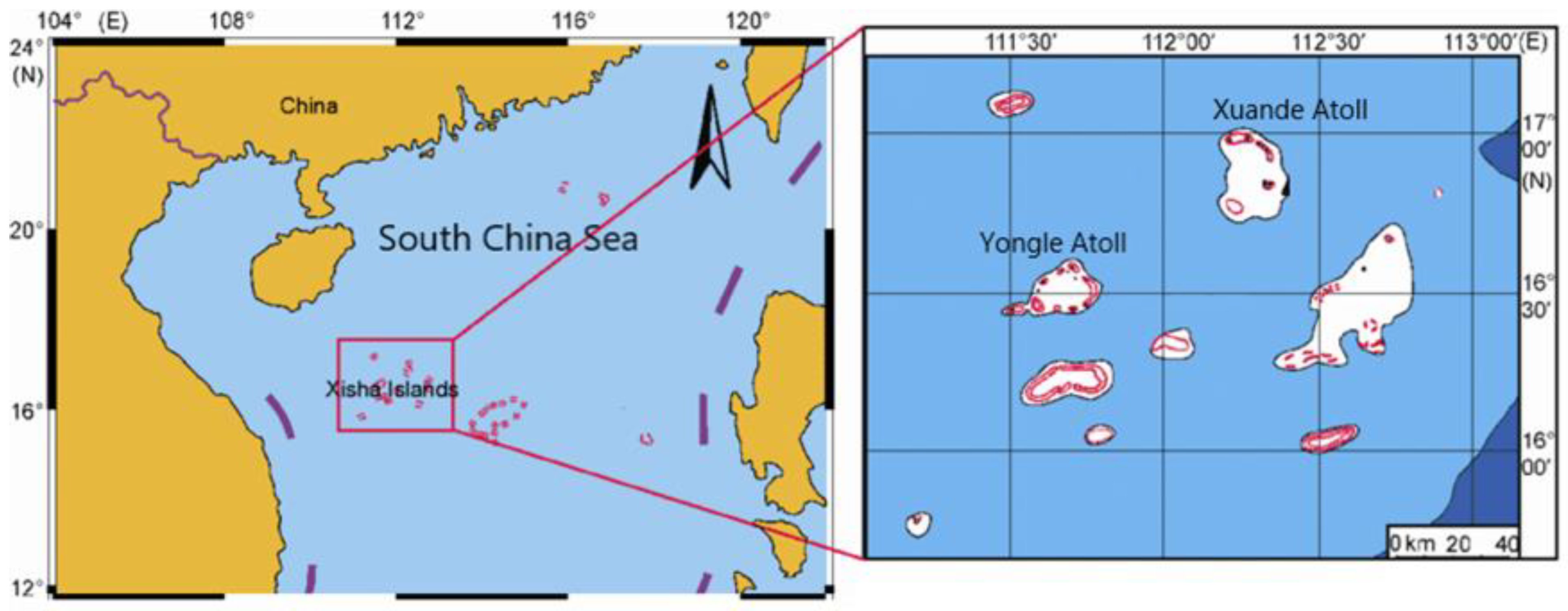
Figure 1. Map of the Xisha Islands in the South China Sea.
Jmse 10 01459 g001
Figure 2. (a) Unstructured grid of the South China Sea. The resolution varies from 3 km to 300 m. (b) Regional numerical grid of the Xisha Islands. The color scale indicates the water depth.
Jmse 10 01459 g002
Figure 3. Geographic location of buoy stations in the Xisha Islands.
Jmse 10 01459 g003
Figure 4. Time-series comparison of hindcast Hs versus buoy-observed Hs. The red circles indicate the procedure of typhoon Kalmeage in 2014.
Jmse 10 01459 g004
Figure 5. Time-series comparison of Hs during Typhoon Kalmaegi in 2014.
Jmse 10 01459 g005
Figure 6. Hourly averaged wind speed (WSD) over the Xisha Islands.
Jmse 10 01459 g006
Figure 7. Seasonal distribution of hourly averaged wind speed (WSD) in the Xisha Islands.
Jmse 10 01459 g007
Figure 8. Distribution of the annual mean Hs in the Xisha Islands.
Jmse 10 01459 g008
Figure 9. Distribution of seasonal mean Hs in the Xisha Islands.
Jmse 10 01459 g009
Figure 10. Distribution of annual mean wind wave ratio coefficient in the Xisha Islands.
Jmse 10 01459 g010
Figure 11. Rose plot of wind speed at the Xisha Islands.
Jmse 10 01459 g011
Figure 12. Monthly wind rose plots of wind speed at the Xisha Islands.
Jmse 10 01459 g012
Figure 13. Reference sites near the Xuande and Yongle Atolls in the Xisha Islands.
Jmse 10 01459 g013
Figure 14. Wave scatter diagram at Site A.
Jmse 10 01459 g014
Figure 15. Wave scatter diagram at Site B.
Jmse 10 01459 g015
Figure 16. Wave scatter diagram at Site C.
Jmse 10 01459 g016
Figure 17. Wave scatter diagram at Site D.
Jmse 10 01459 g017
Figure 18. Wave scatter diagram at Site E.
Jmse 10 01459 g018
Figure 19. Wave scatter diagram at Site F.
Jmse 10 01459 g019
Figure 20. Rose plot of Hs at reference sites in the Xisha Islands.
Jmse 10 01459 g020
Figure 21. Regression curve of the wind speed at the Xisha Islands using the AM-GEV method.
Jmse 10 01459 g021
Figure 22. Monthly distribution of tropical storm tracks affecting the Xisha Islands in the South China Sea from 1988 to 2019.
Jmse 10 01459 g022
Figure 23. Monthly distribution of tropical storm frequency affecting the Xisha Islands.
Jmse 10 01459 g023
Figure 24. Regression curve of the wind speed at the Xisha Islands using POT-GPD method.
Jmse 10 01459 g024
Figure 25. Regression curve of Hs at sites using the AM-GEV method.
Jmse 10 01459 g025
Figure 26. Mean residual life plot for the threshold selection at six sites.
Jmse 10 01459 g026
Figure 27. Regression curve of Hs at sites using POT-GPD method.
Jmse 10 01459 g027
Figure 28. Fitting results of significant wave heights using two-parameter Weibull distribution of sea-state parameters at reference sites in the Xisha Islands.
Jmse 10 01459 g028
Figure 29. Fitting results of significant wave heights using the exponentiated Weibull distribution of sea-state parameters at reference sites in the Xisha Islands.
Jmse 10 01459 g029
Figure 30. Corresponding contour plots of sea-state parameters at reference sites in the Xisha Islands.
Jmse 10 01459 g030aJmse 10 01459 g030b
Table 1. Statistical comparisons between wave WW3 hindcast data and buoy data.
IndexNumber of Sea StatesCorrelationY–X Stdev (m)BiasRoot Mean Square ErrorScatter Index
Buoy116,8150.8810.1190.0210.0870.292
Buoy223710.9040.2060.0760.1590.213
Buoy333120.9220.1670.0250.1160.191
Table 2. Wind speed classification at the Xisha Islands.
MonthFrequency (%)Maximum (m/s)Mean(m/s)Standard Deviation (m/s)
Class < 33 < Class < 66 < Class < 77 < Class < 88 < Class
U < 5.4 m/s5.5 m/s < U < 13.8 m/s13.9 m/s < U < 17.1 m/s17.2 m/s < U < 20.7 m/s20.8 m/s < U
January14.5478.475.271.720.0020.768.783.07
February27.2169.713.040.040.0018.267.543.01
April34.7963.891.280.040.0017.856.662.58
March44.8454.580.540.040.0034.135.932.29
May49.1550.450.180.220.0028.225.672.42
June28.2470.740.480.350.1937.806.842.65
July35.4463.070.980.370.1433.076.512.87
August43.4255.121.010.200.2531.66.163.04
September56.5940.861.460.670.4240.575.513.29
October26.9768.443.110.920.5638.117.763.55
November13.3275.939.261.070.4238.769.563.56
December7.3376.6114.081.880.1035.8810.493.33
Total31.8164.113.400.500.1840.577.283.37
Table 3. Information of six selected near-island locations for wave characterization.
LocationWater Depth (m)
Xuande AtollSite A41.75
Site B41.77
Site C44.25
Yongle AtollSite D52.45
Site E29.91
Site F44.32
Table 4. Hundred-year return level estimation results at six sites.
Xuande AtollYongle Atoll
100-Year Return Level (m)Site ASite BSite CSite DSite ESite F
GEV Lower Bound of 95% confidence intervals8.769.199.207.344.926.61
Best fit13.1013.6914.1410.876.7712.78
Upper Bound of 95% confidence intervals21.9923.1624.8817.969.4325.01
POT-GPDLower Bound of 95% confidence intervals9.409.269.158.176.578.77
Best fit11.4911.2311.4210.707.6515.52
Upper Bound of 95% confidence intervals15.8016.3914.9018.2412.2633.41
Table 5. Fitted parameters using different models at six selected near-island locations.
LocationWeibull DistributionExponentiated Weibull Distribution
α (Scale)Β (Shape)α (Scale)β (Shape1)δ (Shape2)
Xuande AtollSite A1.481.192.772.070.324
Site B1.491.182.621.910.399
Site C1.61.32.321.720.534
Yongle AtollSite D1.051.520.4780.9082.93
Site E0.6871.920.005510.413531
Site F1.051.840.003390.3691500
Table 6. Comparison between extreme value analysis results and environmental contour results at the 100-year return level.
Xuande AtollYongle Atoll
MethodParameterSite ASite BSite CSite DSite ESite F
Environmental ContourHs (m)13.2913.5811.959.257.8212.98
Tz (s)10.8910.8510.7010.258.9811.94
GEVHs (m)13.1013.6914.1410.876.7712.78
POT-GPDHs (m)11.4911.2311.4210.707.6515.52
Publisher’s Note: MDPI stays neutral with regard to jurisdictional claims in published maps and institutional affiliations.