Figure 1.
KCS hull geometry.
Figure 1.
KCS hull geometry.
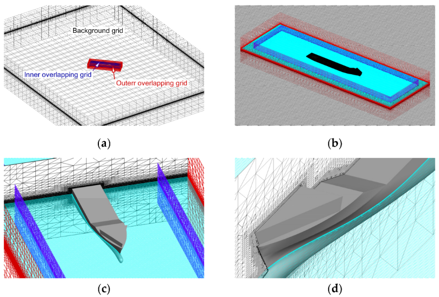
Figure 2.
Overset computational mesh. (a) Global view of the computational domain; (b) global view of the inner computational domain; (c) close-up view of the overlapping inner domain; (d) close-up view of the inner mesh around the hull.
Figure 2.
Overset computational mesh. (a) Global view of the computational domain; (b) global view of the inner computational domain; (c) close-up view of the overlapping inner domain; (d) close-up view of the inner mesh around the hull.
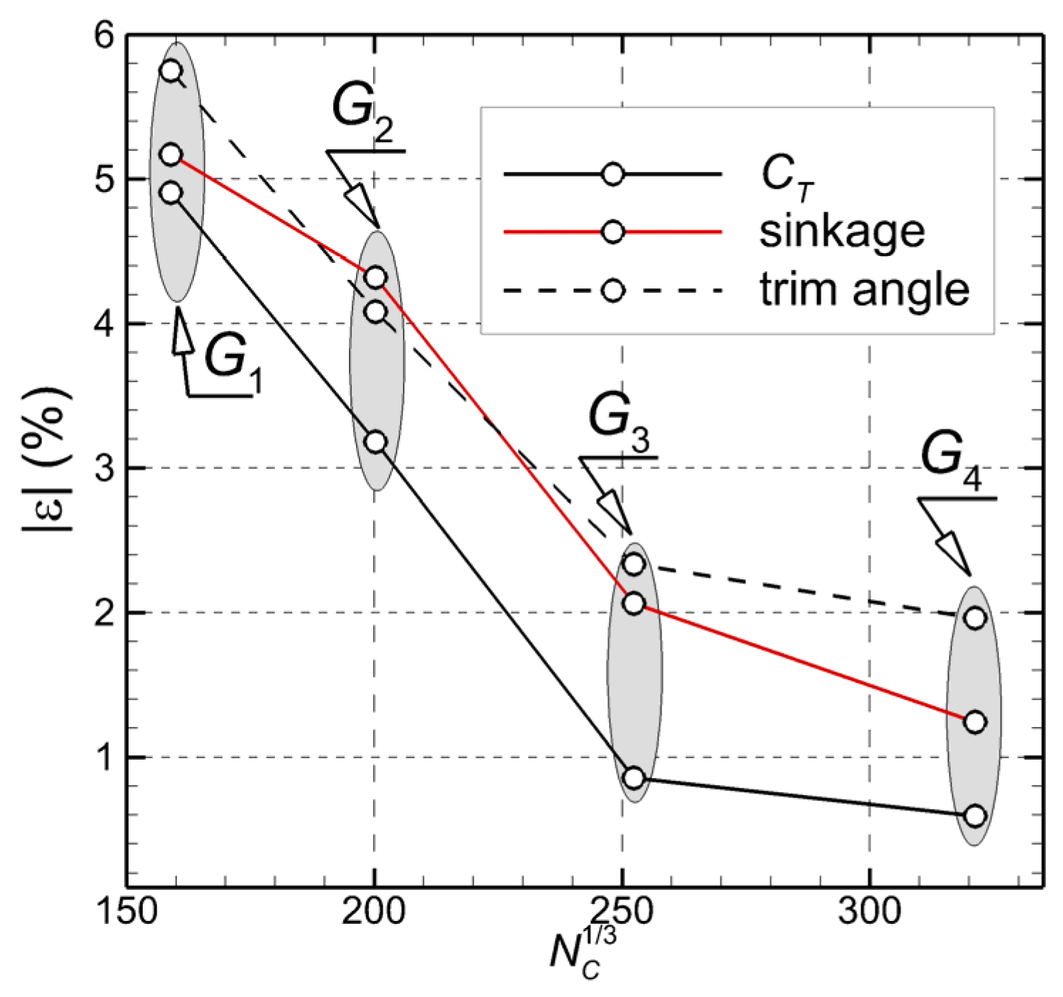
Figure 3.
Grid convergence test.
Figure 3.
Grid convergence test.
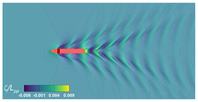
Figure 4.
Free-surface profile computed in calm water at on the finest mesh G3.
Figure 4.
Free-surface profile computed in calm water at on the finest mesh G3.
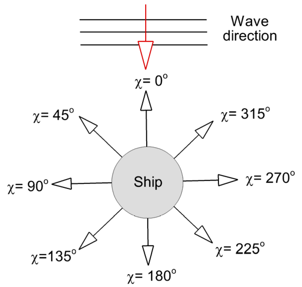
Figure 5.
Relative angle between the ship heading and the wave direction.
Figure 5.
Relative angle between the ship heading and the wave direction.
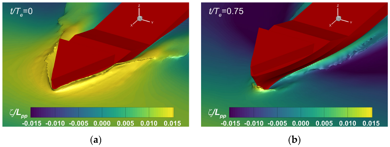
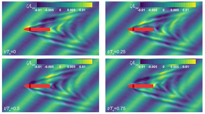
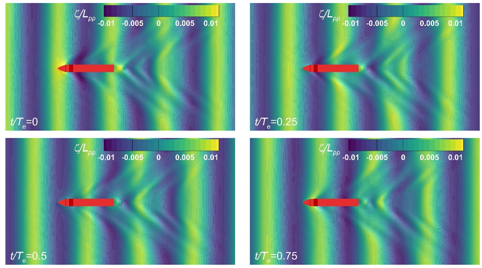
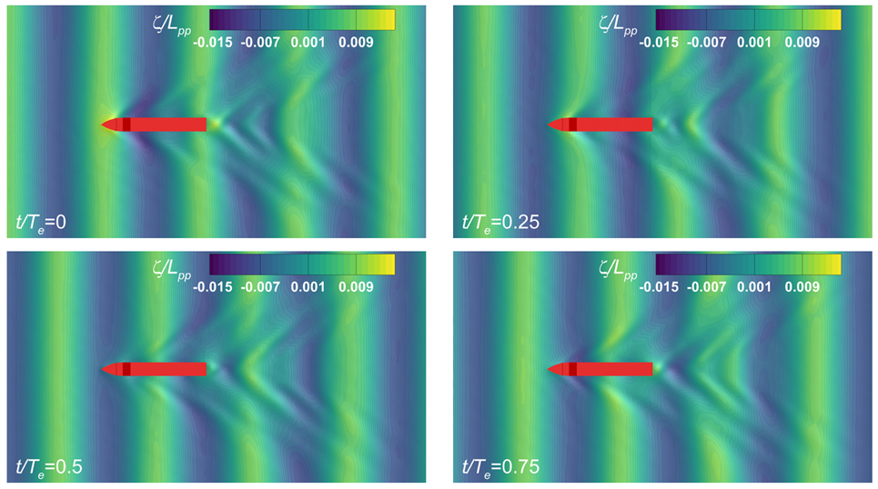
Figure 6.
Free-surface elevations over a period of the head wave encounter.
Figure 6.
Free-surface elevations over a period of the head wave encounter.
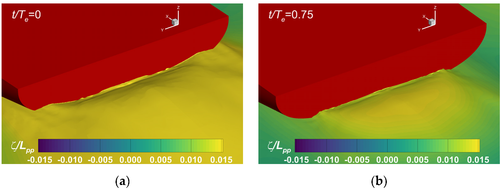
Figure 7.
Bow wave profiles computed in the head sea case at: (a) ; (b) .
Figure 7.
Bow wave profiles computed in the head sea case at: (a) ; (b) .
Figure 8.
Stern wave profiles computed in the head sea case at: (a) ; (b) .
Figure 8.
Stern wave profiles computed in the head sea case at: (a) ; (b) .
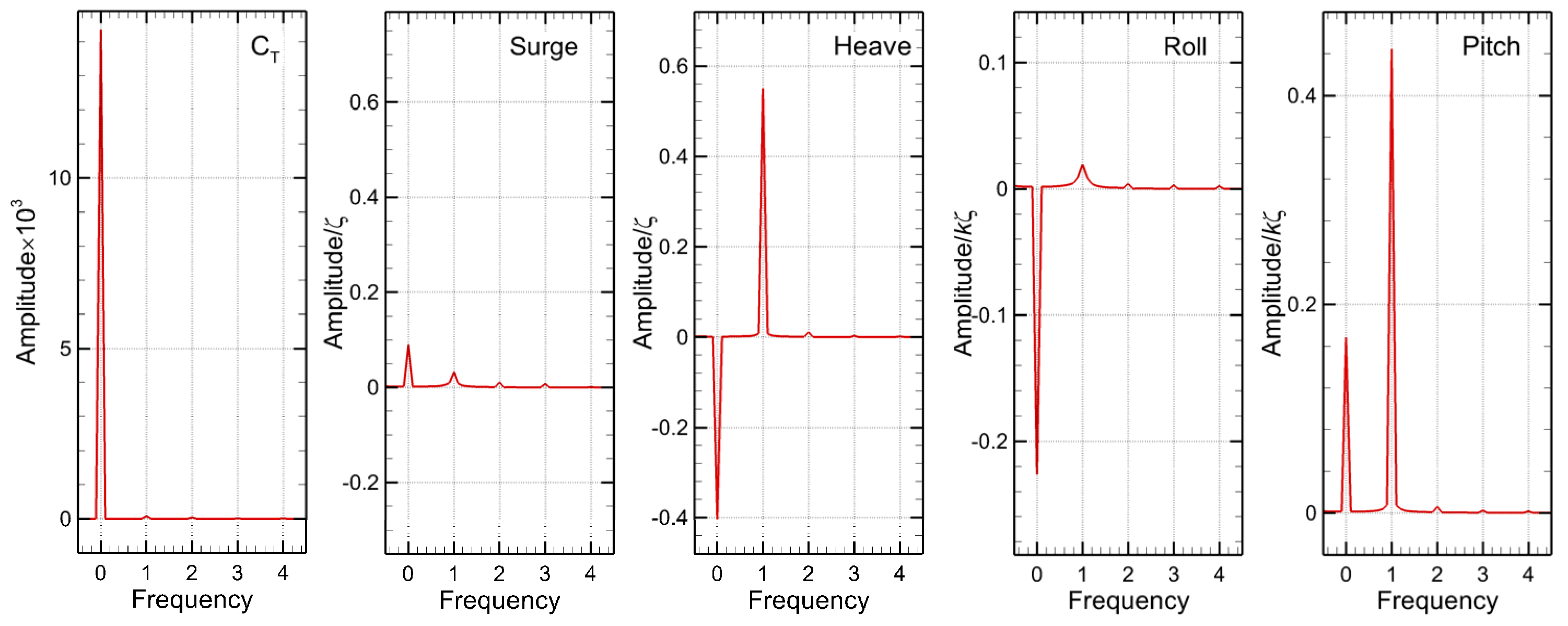
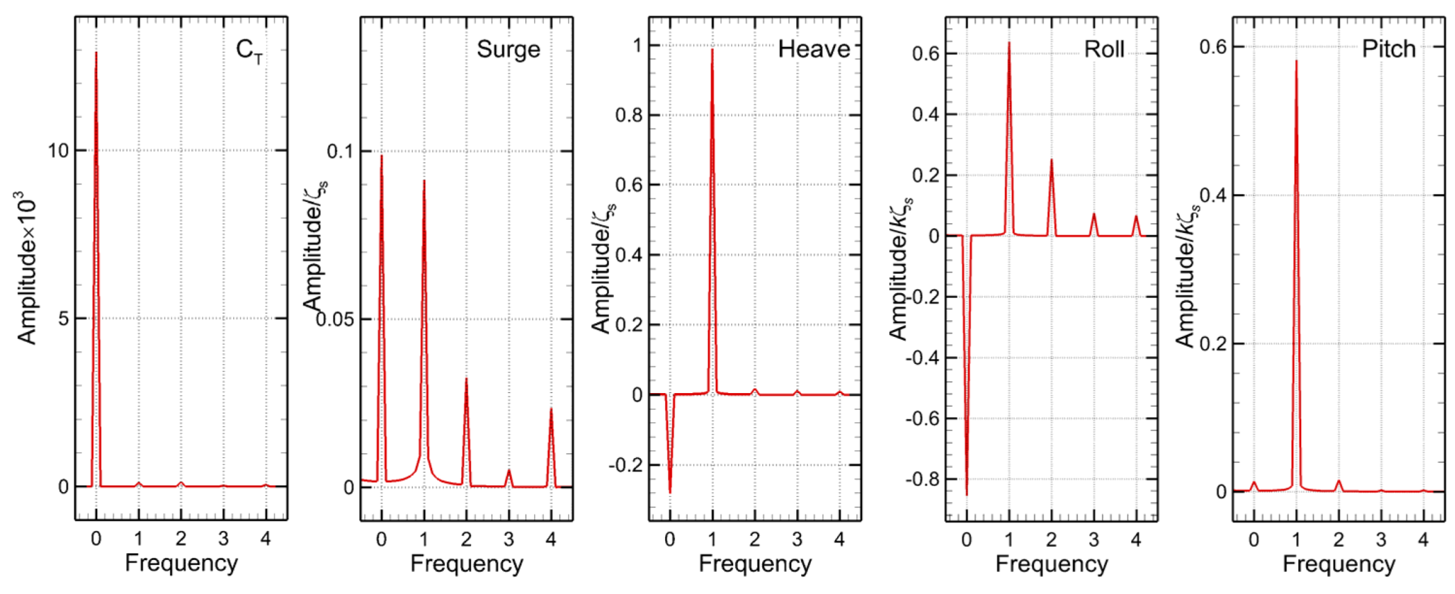
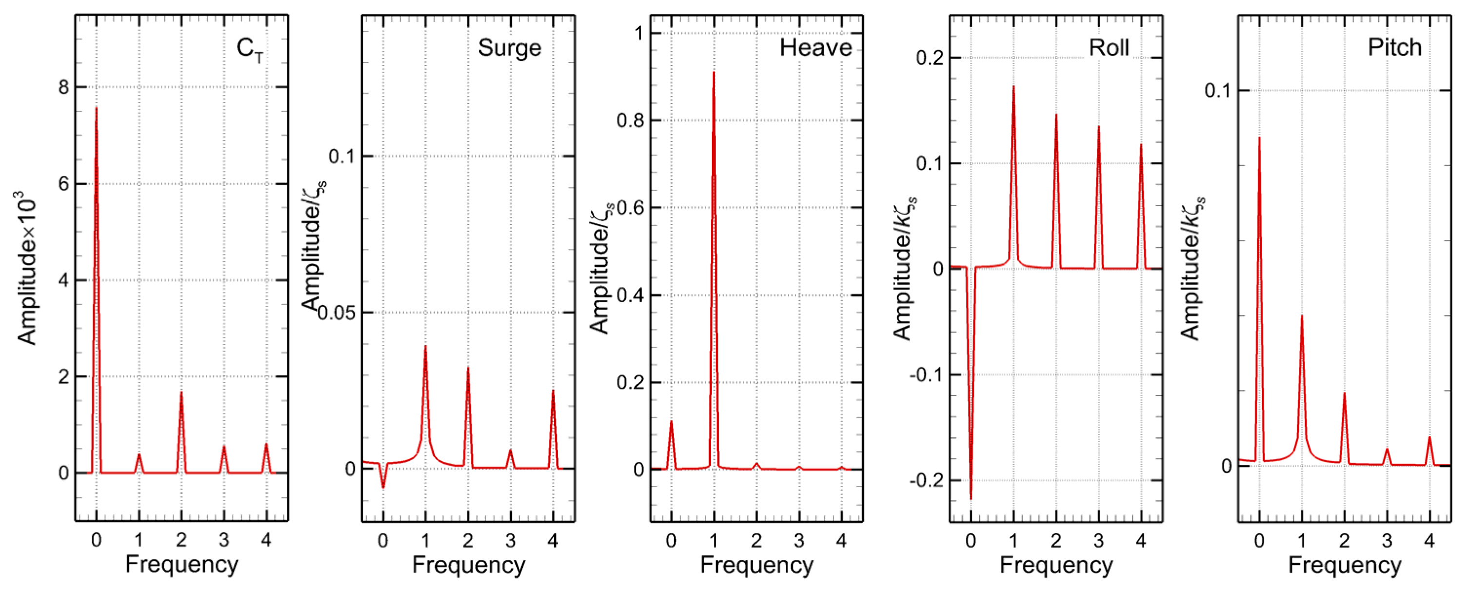
Figure 9.
Harmonic amplitudes of the total resistance coefficient , surge , heave , roll and pitch for the head waves scenario.
Figure 9.
Harmonic amplitudes of the total resistance coefficient , surge , heave , roll and pitch for the head waves scenario.
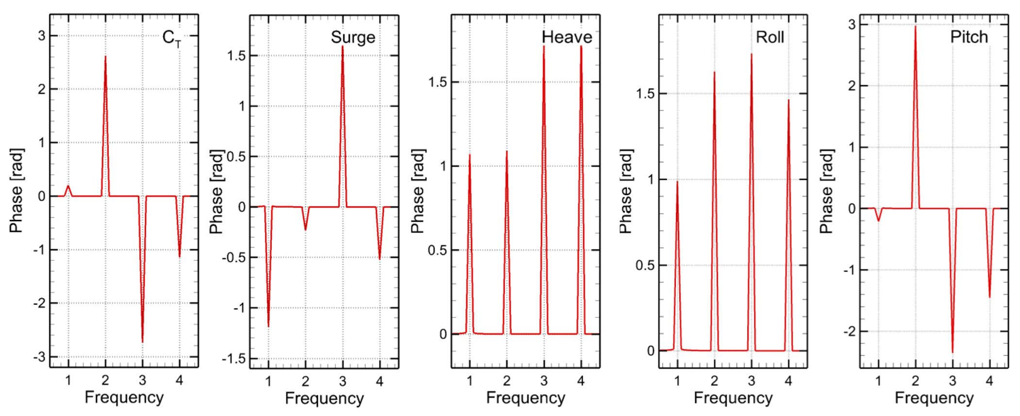
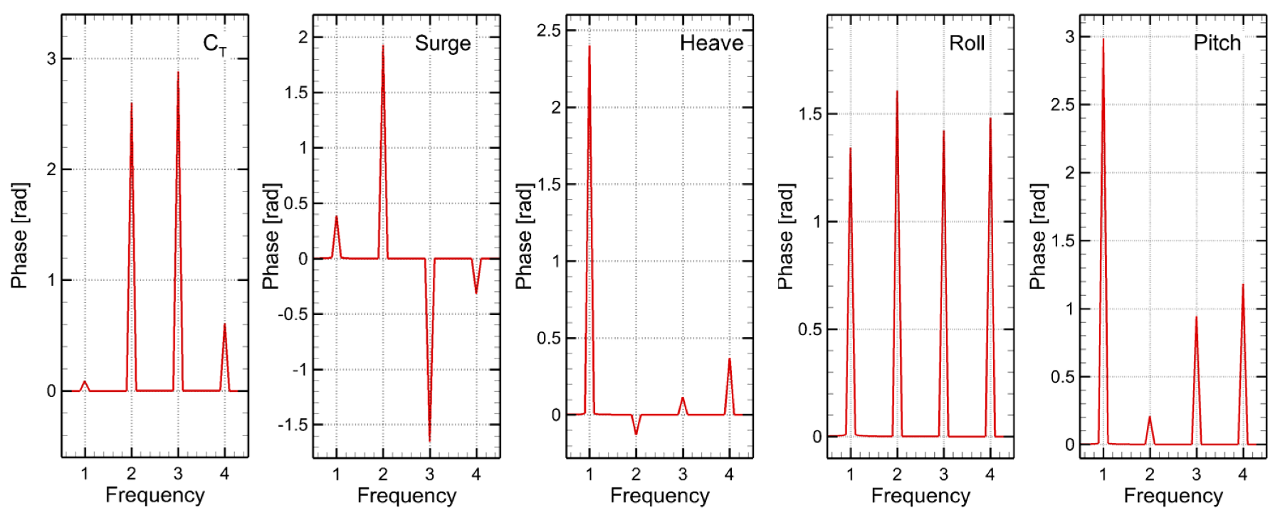
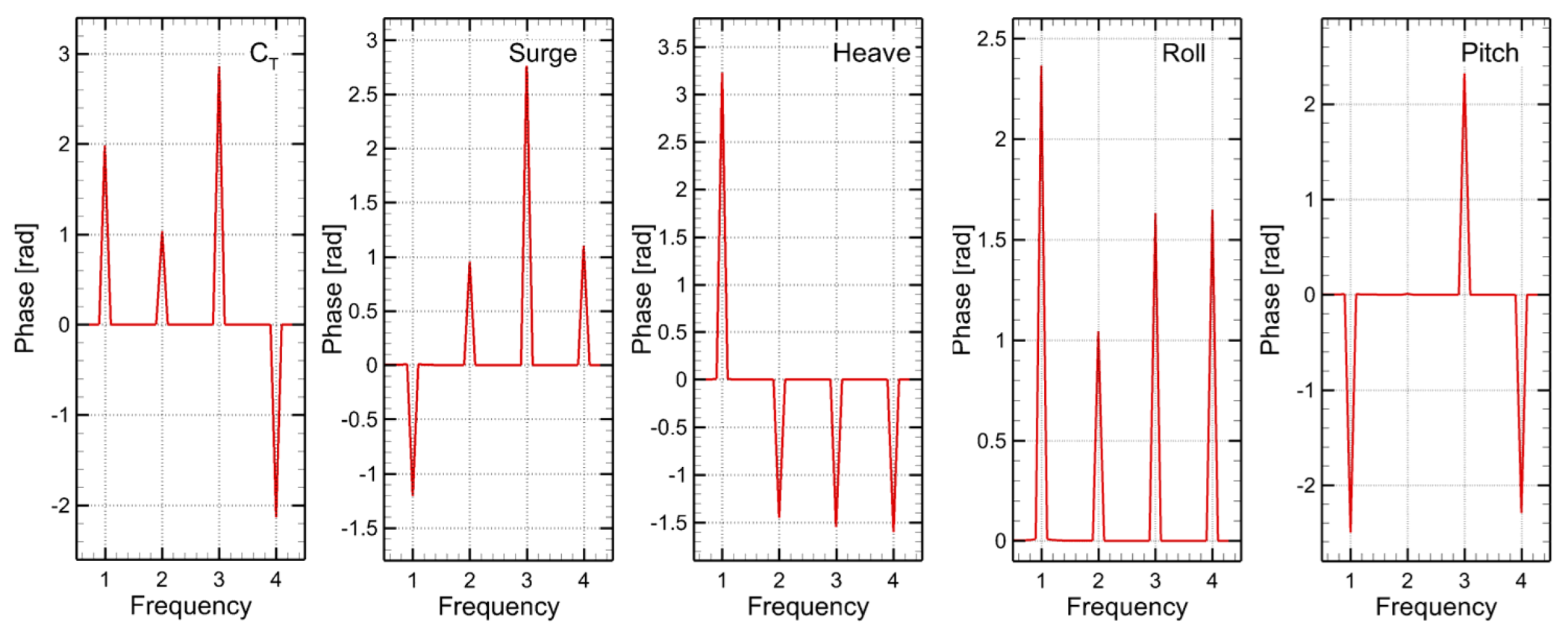
Figure 10.
Harmonic phases of the total resistance coefficient , surge , heave , roll , and pitch for the head waves scenario.
Figure 10.
Harmonic phases of the total resistance coefficient , surge , heave , roll , and pitch for the head waves scenario.
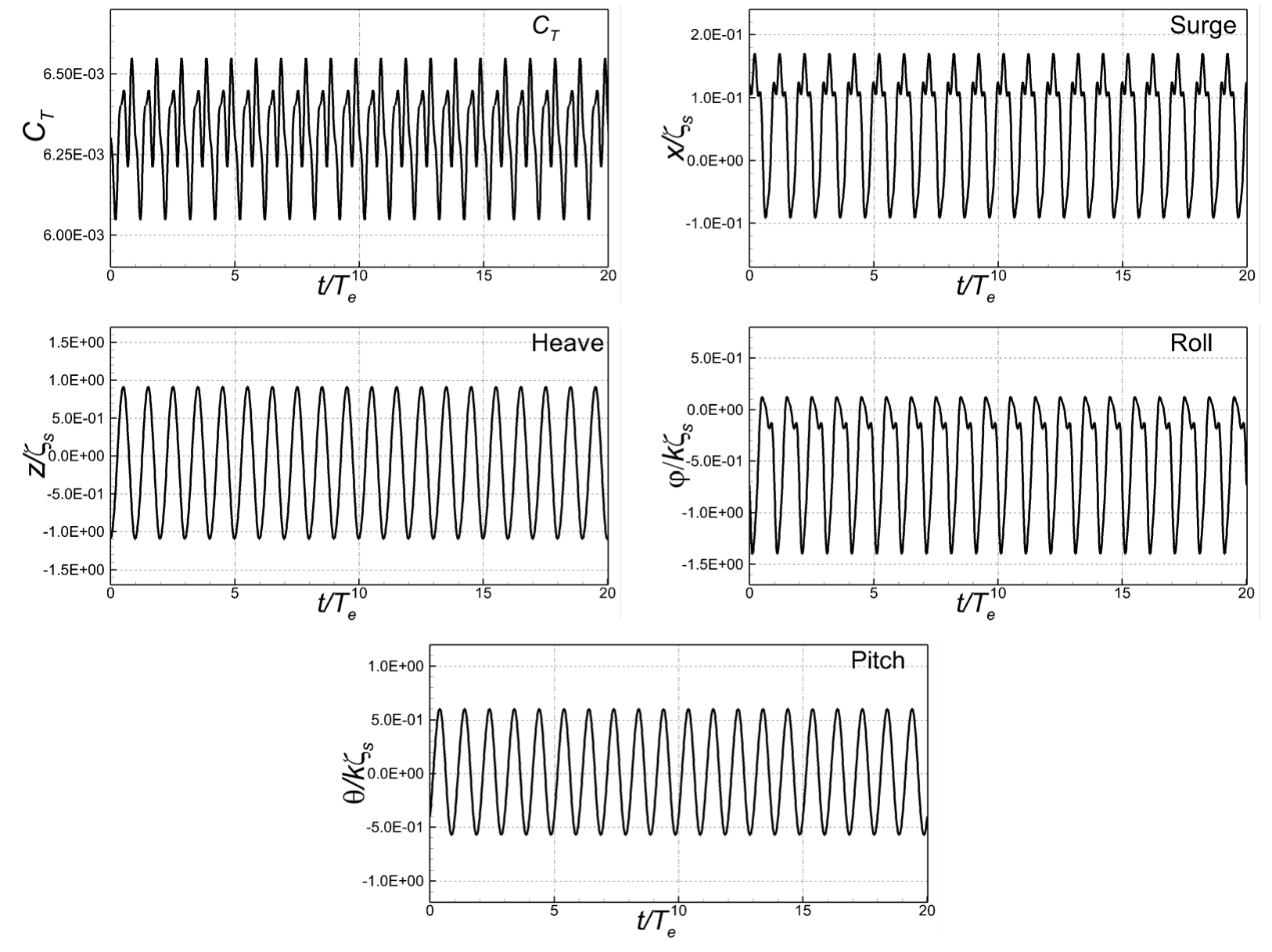
Figure 11.
Time histories of the Fourier reconstructed resistance coefficient , surge , heave , roll and pitch for the head waves scenario.
Figure 11.
Time histories of the Fourier reconstructed resistance coefficient , surge , heave , roll and pitch for the head waves scenario.
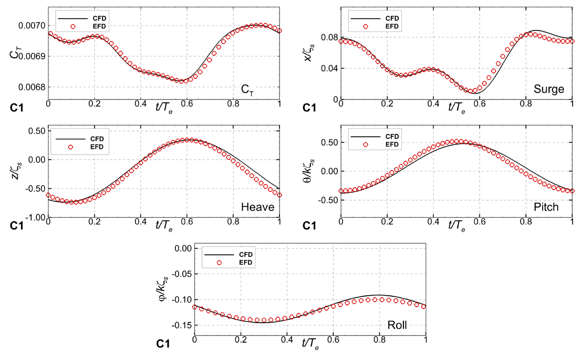
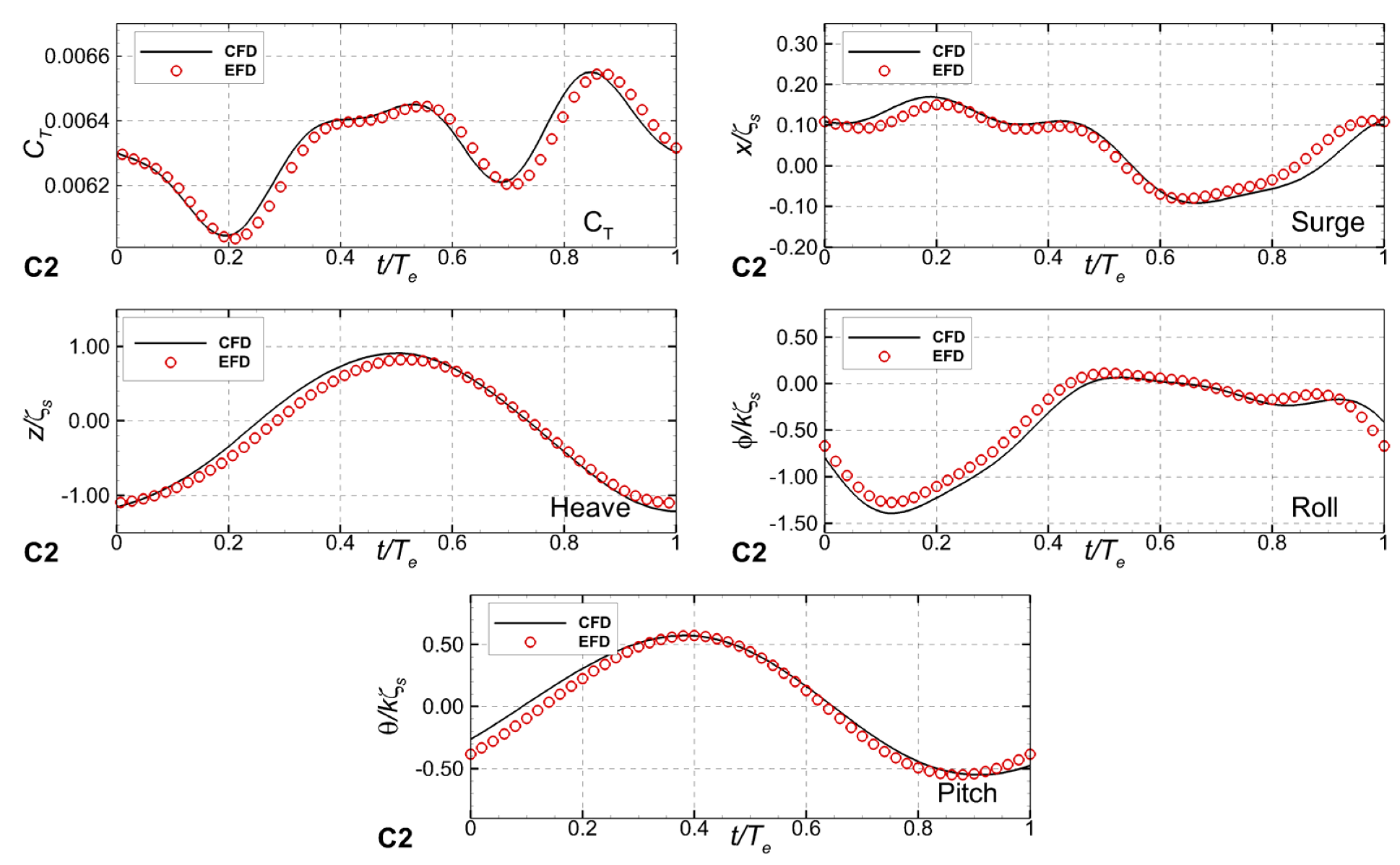
Figure 12.
Comparisons between the time histories of the reconstructed resistance coefficient
surge
, heave
, roll
, and pitch
measured (EFD) [
33] and computed (CFD) over a period of the encounter wave in the
head waves scenario.
Figure 12.
Comparisons between the time histories of the reconstructed resistance coefficient
surge
, heave
, roll
, and pitch
measured (EFD) [
33] and computed (CFD) over a period of the encounter wave in the
head waves scenario.
Figure 13.
Free-surface elevations over a period of the bow wave encounter.
Figure 13.
Free-surface elevations over a period of the bow wave encounter.
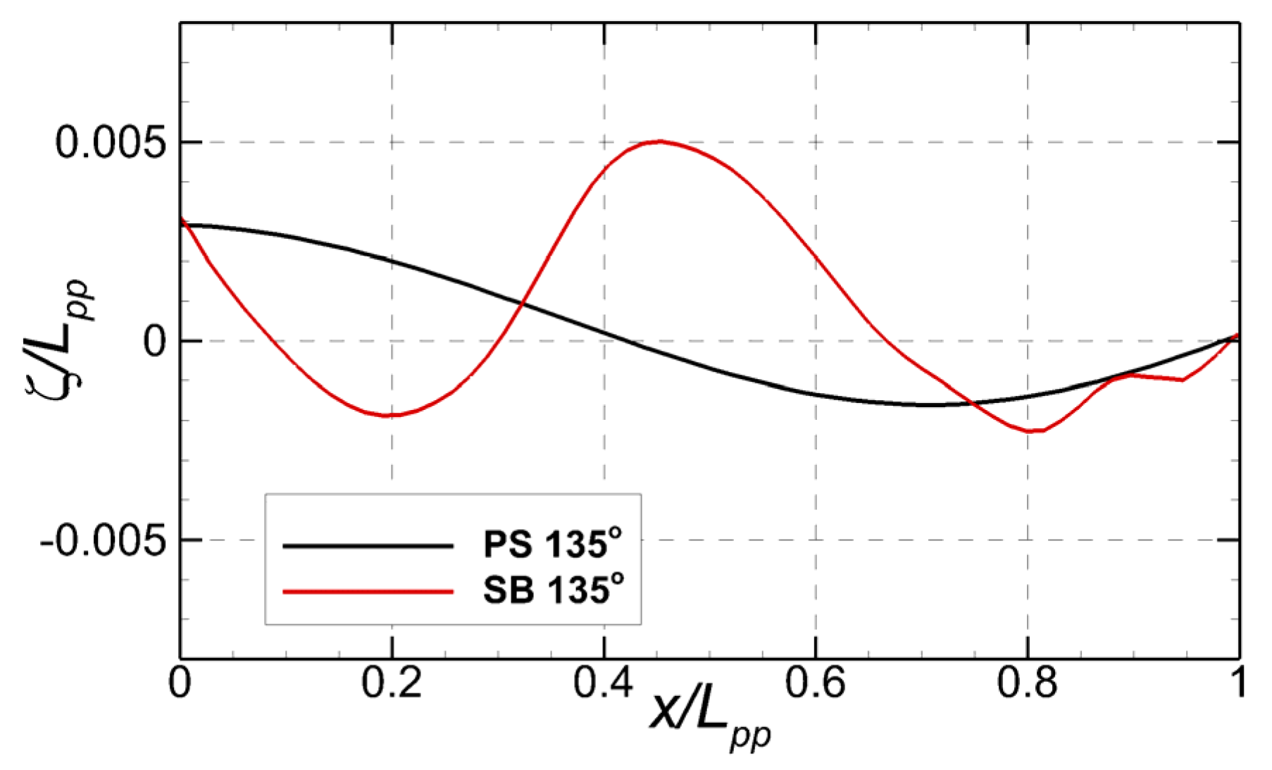
Figure 14.
Wave profiles on the hull.
Figure 14.
Wave profiles on the hull.
Figure 15.
Harmonic amplitudes of the total resistance coefficient , surge , heave , roll , and pitch for the bow waves scenario.
Figure 15.
Harmonic amplitudes of the total resistance coefficient , surge , heave , roll , and pitch for the bow waves scenario.
Figure 16.
Harmonic phases of the total resistance coefficient , surge , heave , roll , and pitch for the bow waves scenario.
Figure 16.
Harmonic phases of the total resistance coefficient , surge , heave , roll , and pitch for the bow waves scenario.
Figure 17.
Time histories of the Fourier reconstructed resistance coefficient , surge , heave , roll and pitch for the bow waves scenario.
Figure 17.
Time histories of the Fourier reconstructed resistance coefficient , surge , heave , roll and pitch for the bow waves scenario.
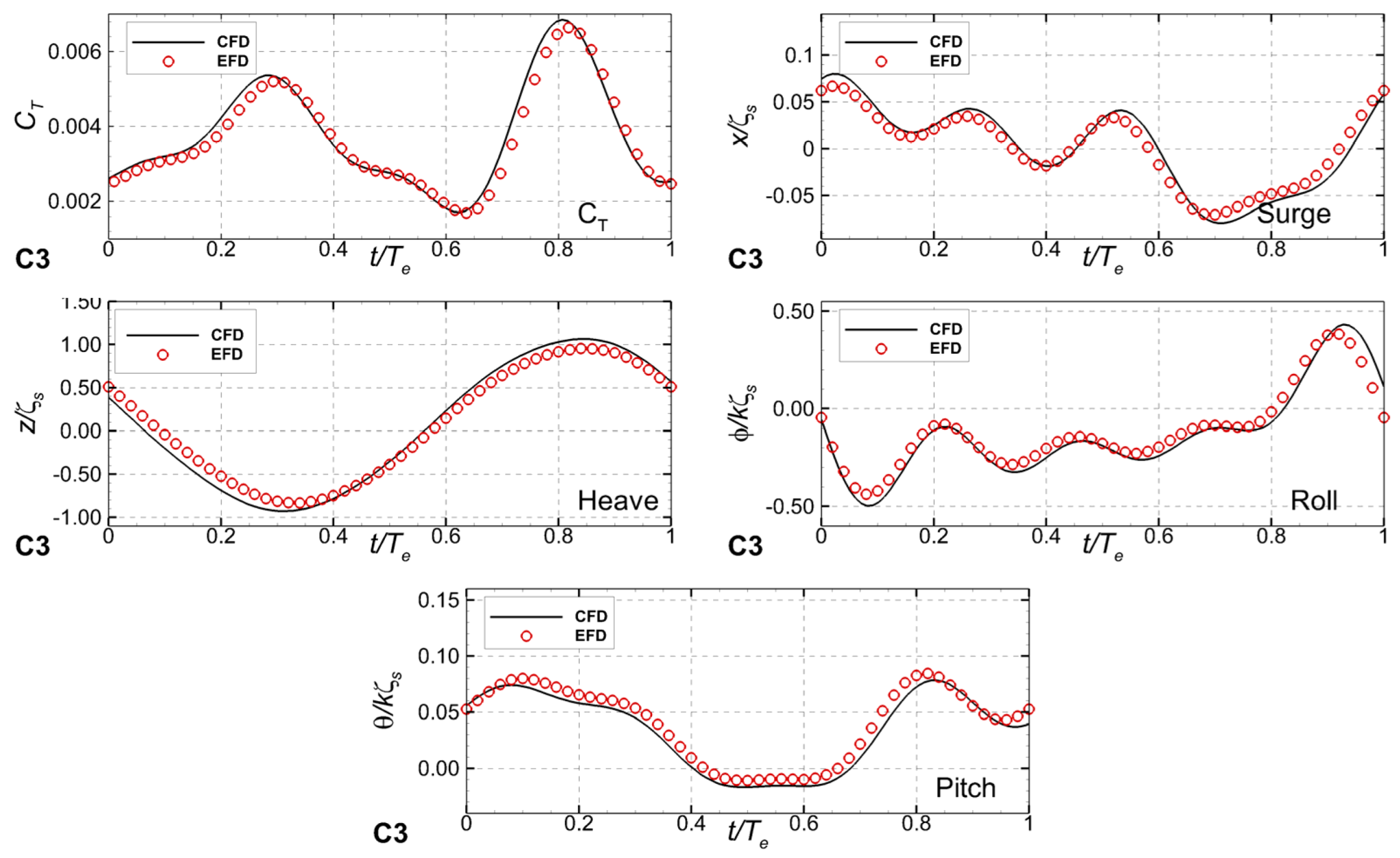
Figure 18.
Comparisons between the time histories of the reconstructed resistance coefficient
surge
, heave
, roll
, and pitch
measured (EFD) [
33] and computed (CFD) over a period of the encounter wave in the
bow waves scenario.
Figure 18.
Comparisons between the time histories of the reconstructed resistance coefficient
surge
, heave
, roll
, and pitch
measured (EFD) [
33] and computed (CFD) over a period of the encounter wave in the
bow waves scenario.
Figure 19.
Free-surface elevations over a period of the beam wave encounter.
Figure 19.
Free-surface elevations over a period of the beam wave encounter.
Figure 20.
Harmonic amplitudes of the total resistance coefficient , surge , heave , roll , and pitch for the beam waves scenario.
Figure 20.
Harmonic amplitudes of the total resistance coefficient , surge , heave , roll , and pitch for the beam waves scenario.
Figure 21.
Harmonic phases of the total resistance coefficient , surge , heave , roll , and pitch for the beam waves scenario.
Figure 21.
Harmonic phases of the total resistance coefficient , surge , heave , roll , and pitch for the beam waves scenario.
Figure 22.
Comparisons between the time histories of the reconstructed resistance coefficient
, surge
, heave
, roll
, and pitch
measured (EFD) [
33], and computed (CFD) over a period of the encounter in the
beam waves scenario.
Figure 22.
Comparisons between the time histories of the reconstructed resistance coefficient
, surge
, heave
, roll
, and pitch
measured (EFD) [
33], and computed (CFD) over a period of the encounter in the
beam waves scenario.
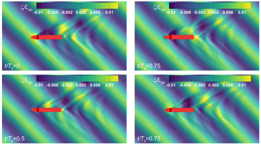
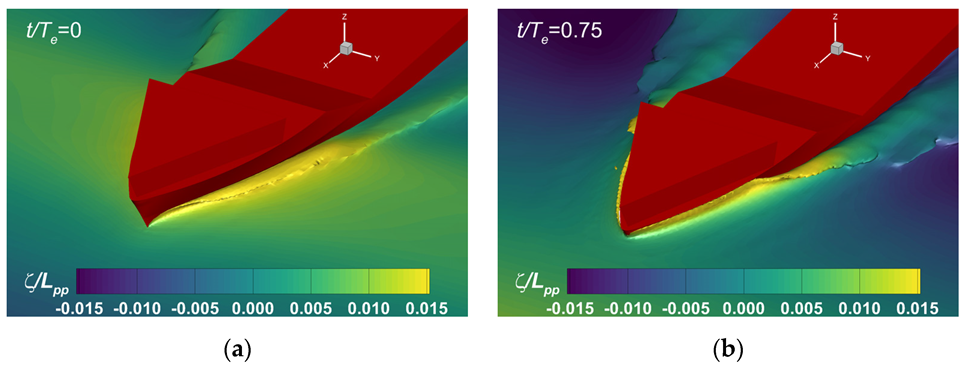
Figure 23.
Free-surface elevations over a period of the quartering wave encounter.
Figure 23.
Free-surface elevations over a period of the quartering wave encounter.
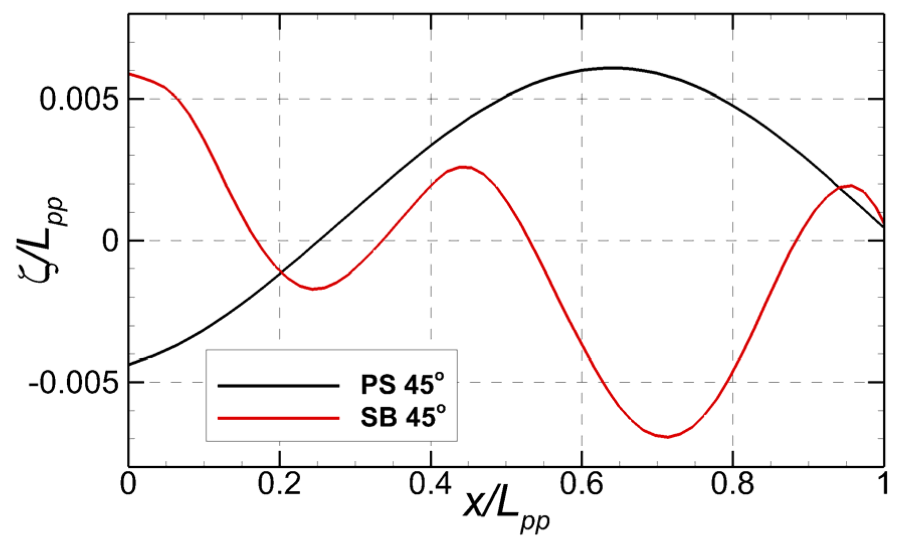
Figure 24.
Wave profiles on the hull.
Figure 24.
Wave profiles on the hull.
Figure 25.
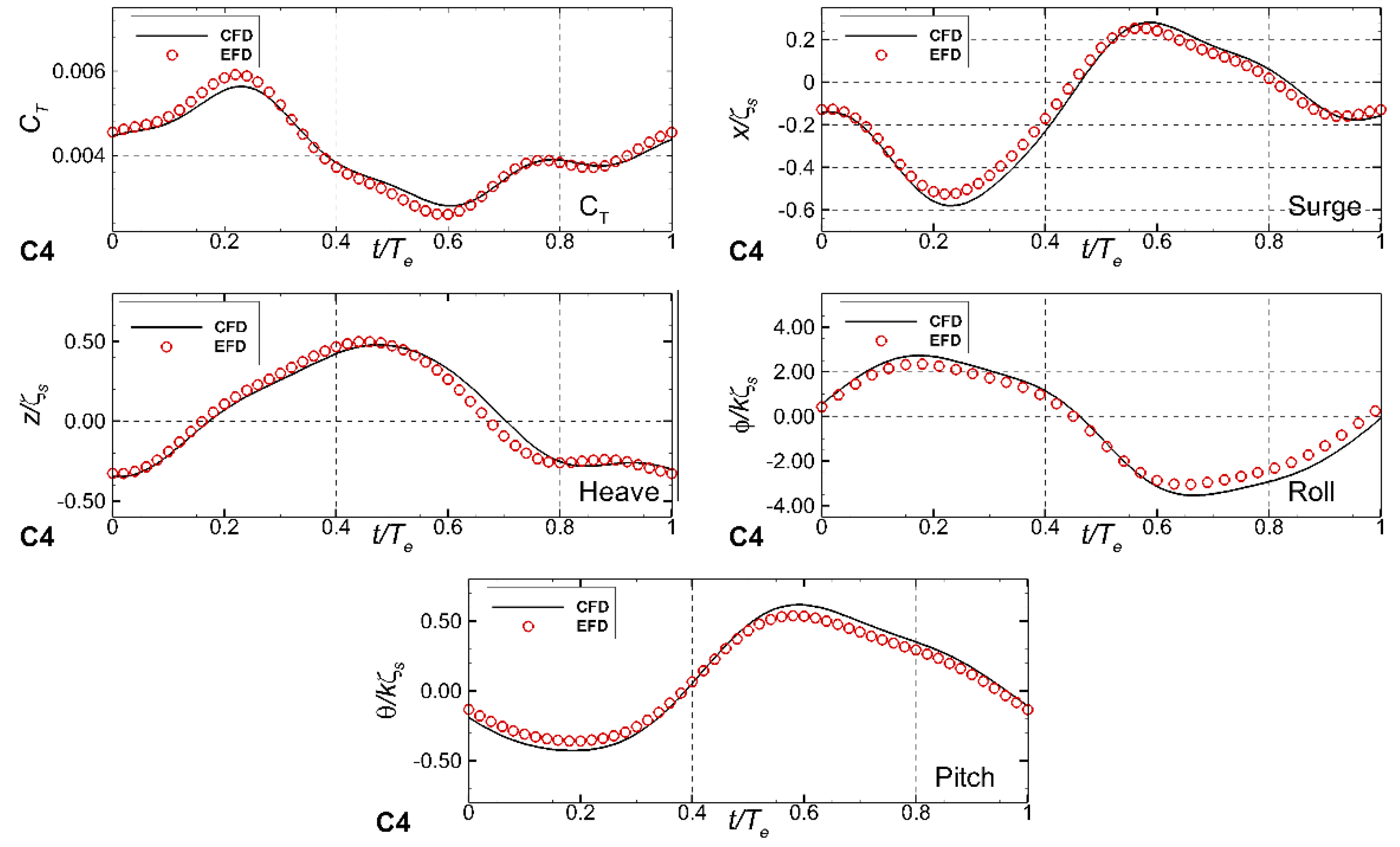
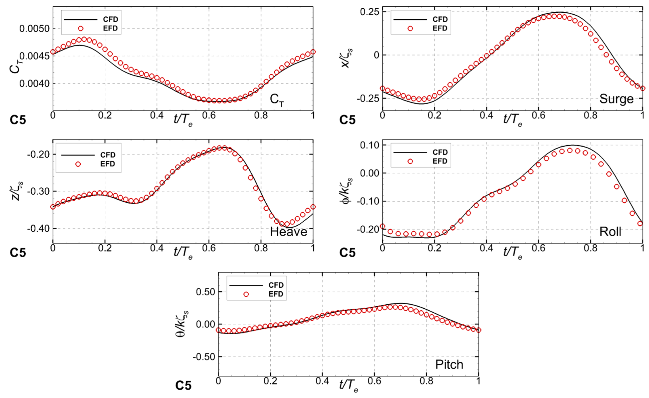
Comparisons between the time histories of the reconstructed resistance coefficient
, surge
, heave
, roll
, and pitch
measured (EFD) [
33], and computed (CFD) over a period of the encounter in the
quartering waves scenario.
Figure 25.
Comparisons between the time histories of the reconstructed resistance coefficient
, surge
, heave
, roll
, and pitch
measured (EFD) [
33], and computed (CFD) over a period of the encounter in the
quartering waves scenario.
Figure 26.
Free-surface elevations over a period of the following wave encounter.
Figure 26.
Free-surface elevations over a period of the following wave encounter.
Figure 27.
Bow wave profiles computed in the head sea case at: (a) ; (b) .
Figure 27.
Bow wave profiles computed in the head sea case at: (a) ; (b) .
Figure 28.
Comparisons between the time histories of the reconstructed resistance coefficient
, surge
, heave
, roll
, and pitch
measured (EFD) [
33], and computed (CFD) over a period of the encounter in the
following waves scenario.
Figure 28.
Comparisons between the time histories of the reconstructed resistance coefficient
, surge
, heave
, roll
, and pitch
measured (EFD) [
33], and computed (CFD) over a period of the encounter in the
following waves scenario.
Table 1.
Main particulars of the ship hull.
Table 1.
Main particulars of the ship hull.
| Main Particulars | Symbol | Full Scale | Model Scale |
|---|
| Length between perpendiculars | [m] | 230 | 2.7 |
| Length of waterline | [m] | 232.5 | 2.729 |
| Maximum beam of waterline | [m] | 32.2 | 0.378 |
| Depth | [m] | 19.0 | 0.223 |
| Draft | [m] | 10.8 | 0.1268 |
| Displacement volume | ∇ [m3] | 5203 | 0.084 |
| Wetted surface area w/o rudder | [m2] | 9424 | 1.31 |
| Wetted surface area of rudder | [m2] | 115.0 | 0.016 |
| | 0.6505 | 0.651 |
| ), fwd+ | | −1.48 | −1.48 |
| Vertical center of gravity (from keel) | [m] | | 0.168 |
| Moment of inertia | | 0.4 | 0.39 |
| Moment of inertia | | 0.25 | 0.25 |
Table 2.
Grid sensitivity study for the mean values of the total resistance coefficient, sinkage, and trim computed in calm water.
Table 2.
Grid sensitivity study for the mean values of the total resistance coefficient, sinkage, and trim computed in calm water.
| | 103 × CT | | Pitch/kζS |
|---|
| | G1 | G2 | G3 | G4 | G1 | G2 | G3 | G4 | G1 | G2 | G3 | G4 |
|---|
| EFD | 4.66 | −1.76 | 0.12 |
| CFD | 4.3314 | 4.5118 | 4.6201 | 4.739 | −1.669 | −1.684 | −1.724 | −1.746 | 0.1131 | 0.1151 | 0.1172 | 0.1194 |
| |ε|%D | 4.906 | 3.180 | 0.856 | 0.593 | 5.170 | 4.318 | 2.063 | 1.241 | 5.751 | 4.083 | 2.333 | 1.963 |
Table 3.
Verification and validation for the total resistance coefficient.
Table 3.
Verification and validation for the total resistance coefficient.
| Parameters | | | | | | |
|---|
| 2.062 | 2.51 | 1.078 | 1.271 | 1.16 | 1.721 |
Table 4.
Harmonic amplitudes and phases of the total resistance coefficient for the head waves scenario.
Table 4.
Harmonic amplitudes and phases of the total resistance coefficient for the head waves scenario.
| Amplitude × 103 | Phase [Rad] |
|---|
| 0th | 1st | 2nd | 3rd | 4th | 1st | 2nd | 3rd | 4th |
|---|
| EFD | 13.8360 | 0.0810 | 0.0330 | 0.0060 | 0.0100 | 0.0888 | 2.5202 | 2.7833 | 0.6501 |
| CFD | 14.1362 | 0.0829 | 0.0342 | 0.0057 | 0.0107 | 0.0913 | 2.5994 | 2.8843 | 0.6131 |
| |ε|% | 2.17% | 2.37% | 3.76% | 5.02% | 7.08% | 2.74% | 3.14% | 3.63% | 5.69% |
Table 5.
Harmonic amplitudes and phases of surge for the head waves scenario.
Table 5.
Harmonic amplitudes and phases of surge for the head waves scenario.
| Amplitude × 103 | Phase [Rad] |
|---|
| 0th | 1st | 2nd | 3rd | 4th | 1st | 2nd | 3rd | 4th |
|---|
| EFD | 0.0924 | 0.0337 | 0.0114 | 0.0074 | 0.0007 | 0.4007 | 1.8750 | −1.5647 | −0.2986 |
| CFD | 0.0902 | 0.0325 | 0.0108 | 0.0078 | 0.0008 | 0.3912 | 1.9289 | −1.6539 | −0.3196 |
| |ε|% | 2.45% | 3.49% | 4.76% | 5.77% | 8.02% | 2.37% | 2.87% | 5.70% | 7.04% |
Table 6.
Harmonic amplitudes and phases of heave for the head waves scenario.
Table 6.
Harmonic amplitudes and phases of heave for the head waves scenario.
| Amplitude × 103 | Phase [Rad] |
|---|
| 0th | 1st | 2nd | 3rd | 4th | 1st | 2nd | 3rd | 4th |
|---|
| EFD | −0.3955 | 0.5356 | 0.0122 | 0.0028 | 0.0014 | 1.4488 | −0.1235 | 0.1097 | 0.3958 |
| CFD | −0.4050 | 0.5501 | 0.0116 | 0.0030 | 0.0015 | 2.4019 | −0.1284 | 0.1152 | 0.3722 |
| |ε|% | 2.39% | 2.71% | 4.91% | 5.17% | 7.33% | 2.71% | 3.92% | 4.96% | 5.96% |
Table 7.
Harmonic amplitudes and phases of roll for the head waves scenario.
Table 7.
Harmonic amplitudes and phases of roll for the head waves scenario.
| Amplitude × 103 | Phase [Rad] |
|---|
| 0th | 1st | 2nd | 3rd | 4th | 1st | 2nd | 3rd | 4th |
|---|
| EFD | −0.2327 | 0.0204 | 0.0040 | 0.0029 | 0.0022 | 1.3018 | 1.5430 | 1.3560 | 1.4093 |
| CFD | −0.2262 | 0.0196 | 0.0043 | 0.0031 | 0.0024 | 1.3431 | 1.6074 | 1.4219 | 1.4808 |
| |ε|% | 2.80% | 3.63% | 5.42% | 7.44% | 8.84% | 3.17% | 4.18% | 4.86% | 5.08% |
Table 8.
Harmonic amplitudes and phases of pitch for the head waves scenario.
Table 8.
Harmonic amplitudes and phases of pitch for the head waves scenario.
| Amplitude × 103 | Phase [Rad] |
|---|
| 0th | 1st | 2nd | 3rd | 4th | 1st | 2nd | 3rd | 4th |
|---|
| EFD | 0.1636 | 0.4303 | 0.0062 | 0.0024 | 0.0016 | 3.1058 | 0.2210 | 1.0053 | 1.2894 |
| CFD | 0.1680 | 0.4446 | 0.0065 | 0.0025 | 0.0018 | 2.9865 | 0.2101 | 0.9448 | 1.1847 |
| |ε|% | 2.65% | 3.32% | 4.71% | 5.84% | 7.71% | 3.84% | 4.91% | 6.02% | 8.12% |
Table 9.
Harmonic amplitudes and phases of the total resistance coefficient for the bow waves scenario.
Table 9.
Harmonic amplitudes and phases of the total resistance coefficient for the bow waves scenario.
| Amplitude × 103 | Phase [Rad] |
|---|
| 0th | 1st | 2nd | 3rd | 4th | 1st | 2nd | 3rd | 4th |
|---|
| EFD | 12.6500 | 0.1100 | 0.1380 | 0.0290 | 0.0560 | 1.9280 | 0.9919 | 3.0171 | −2.0066 |
| CFD | 12.9435 | 0.1132 | 0.1447 | 0.0310 | 0.0509 | 1.9827 | 1.0327 | 2.8599 | −2.1346 |
| |ε|% | 2.32% | 2.95% | 4.83% | 7.02% | 9.11% | 2.84% | 4.11% | 5.21% | 6.38% |
Table 10.
Harmonic amplitudes and phases of surge for the bow waves scenario.
Table 10.
Harmonic amplitudes and phases of surge for the bow waves scenario.
| Amplitude × 103 | Phase [rad] |
|---|
| 0th | 1st | 2nd | 3rd | 4th | 1st | 2nd | 3rd | 4th |
|---|
| EFD | 0.1016 | 0.0951 | 0.0342 | 0.0056 | 0.0219 | −1.1686 | 0.9179 | 2.6984 | 1.0345 |
| CFD | 0.0989 | 0.0913 | 0.0325 | 0.0053 | 0.0236 | −1.2043 | 0.9539 | 2.8336 | 1.1040 |
| |ε|% | 2.61% | 4.02% | 5.12% | 6.23% | 8.11% | 3.06% | 3.92% | 5.01% | 6.71% |
Table 11.
Harmonic amplitudes and phases of heave for the bow waves scenario.
Table 11.
Harmonic amplitudes and phases of heave for the bow waves scenario.
| Amplitude ×103 | Phase [Rad] |
|---|
| 0th | 1st | 2nd | 3rd | 4th | 1st | 2nd | 3rd | 4th |
|---|
| EFD | −0.2769 | 0.9612 | 0.0163 | 0.0103 | 0.0080 | 3.1183 | −1.4002 | −1.4883 | −1.5157 |
| CFD | −0.2825 | 0.9895 | 0.0170 | 0.0108 | 0.0086 | 3.2311 | −1.4524 | −1.5491 | −1.6007 |
| |ε|% | 2.02% | 2.94% | 4.32% | 5.11% | 6.69% | 3.62% | 3.73% | 4.09% | 5.61% |
Table 12.
Harmonic amplitudes and phases of roll for the bow waves scenario.
Table 12.
Harmonic amplitudes and phases of roll for the bow waves scenario.
| Amplitude × 103 | Phase [Rad] |
|---|
| 0th | 1st | 2nd | 3rd | 4th | 1st | 2nd | 3rd | 4th |
|---|
| EFD | −0.8293 | 0.6130 | 0.2416 | 0.0700 | 0.0615 | 2.2674 | 0.9961 | 1.5345 | 1.5134 |
| CFD | −0.8556 | 0.6375 | 0.2541 | 0.0756 | 0.0683 | 2.3651 | 1.0458 | 1.6313 | 1.6494 |
| |ε|% | 3.17% | 3.99% | 5.17% | 7.92% | 11.02% | 4.31% | 4.99% | 6.31% | 8.99% |
Table 13.
Harmonic amplitudes and phases of pitch for the bow waves scenario.
Table 13.
Harmonic amplitudes and phases of pitch for the bow waves scenario.
| Amplitude × 103 | Phase [Rad] |
|---|
| 0th | 1st | 2nd | 3rd | 4th | 1st | 2nd | 3rd | 4th |
|---|
| EFD | 0.0138 | 0.5571 | 0.0151 | 0.0017 | 0.0017 | −2.4041 | 0.0101 | 2.4799 | −2.5035 |
| CFD | 0.0143 | 0.5818 | 0.0159 | 0.0018 | 0.0019 | −2.5007 | 0.0095 | 2.3229 | −2.2927 |
| |ε|% | 3.23% | 4.44% | 5.02% | 6.87% | 8.31% | 4.02% | 5.07% | 6.33% | 8.42% |
Table 14.
Harmonic amplitudes and phases of the total resistance coefficient for the beam waves scenario.
Table 14.
Harmonic amplitudes and phases of the total resistance coefficient for the beam waves scenario.
| Amplitude × 103 | Phase [Rad] |
|---|
| 0th | 1st | 2nd | 3rd | 4th | 1st | 2nd | 3rd | 4th |
|---|
| EFD | 7.4160 | 0.3890 | 1.6300 | 0.5360 | 0.5810 | 0.1950 | 2.5189 | −2.6203 | −1.0904 |
| CFD | 7.5731 | 0.4009 | 1.6932 | 0.5584 | 0.6113 | 0.2004 | 2.6232 | −2.7458 | −1.1476 |
| |ε|% | 2.12% | 3.07% | 3.88% | 4.17% | 5.22% | 2.77% | 4.14% | 4.79% | 5.25% |
Table 15.
Harmonic amplitudes and phases of surge for the beam waves scenario.
Table 15.
Harmonic amplitudes and phases of surge for the beam waves scenario.
| Amplitude × 103 | Phase [Rad] |
|---|
| 0th | 1st | 2nd | 3rd | 4th | 1st | 2nd | 3rd | 4th |
|---|
| EFD | −0.0062 | 0.0379 | 0.0308 | 0.0058 | 0.0235 | −1.1552 | −0.2225 | 1.5693 | −0.5594 |
| CFD | −0.0064 | 0.0394 | 0.0324 | 0.0062 | 0.0254 | −1.1902 | −0.2320 | 1.6448 | −0.5262 |
| |ε|% | 2.56% | 4.14% | 5.19% | 6.16% | 7.92% | 3.03% | 4.26% | 4.81% | 5.92% |
Table 16.
Harmonic amplitudes and phases of heave for the beam waves scenario.
Table 16.
Harmonic amplitudes and phases of heave for the beam waves scenario.
| Amplitude × 103 | Phase [Rad] |
|---|
| 0th | 1st | 2nd | 3rd | 4th | 1st | 2nd | 3rd | 4th |
|---|
| EFD | 0.1106 | 0.8852 | 0.0143 | 0.0075 | 0.0054 | 1.0423 | 1.0542 | 1.7822 | 1.9139 |
| CFD | 0.1130 | 0.9117 | 0.0149 | 0.0071 | 0.0050 | 1.0696 | 1.0901 | 1.7219 | 1.7983 |
| |ε|% | 2.14% | 2.99% | 4.56% | 5.83% | 7.03% | 2.62% | 3.41% | 3.38% | 6.04% |
Table 17.
Harmonic amplitudes and phases of roll for the beam waves scenario.
Table 17.
Harmonic amplitudes and phases of roll for the beam waves scenario.
| Amplitude × 103 | Phase [Rad] |
|---|
| 0th | 1st | 2nd | 3rd | 4th | 1st | 2nd | 3rd | 4th |
|---|
| EFD | −0.2130 | 0.1663 | 0.1396 | 0.1264 | 0.1093 | 0.9576 | 1.5774 | 1.8198 | 1.5657 |
| CFD | −02191 | 0.1735 | 0.1464 | 0.1351 | 0.1185 | 0.9905 | 1.6274 | 1.7328 | 1.4662 |
| |ε|% | 2.88% | 4.34% | 6492% | 6.92% | 8.41% | 3.44% | 3.17% | 4.78% | 6.35% |
Table 18.
Harmonic amplitudes and phases of pitch for the beam waves scenario.
Table 18.
Harmonic amplitudes and phases of pitch for the beam waves scenario.
| Amplitude × 103 | Phase [Rad] |
|---|
| 0th | 1st | 2nd | 3rd | 4th | 1st | 2nd | 3rd | 4th |
|---|
| EFD | 0.0846 | 0.0386 | 0.0186 | 0.0052 | 0.0086 | −0.2014 | 2.8975 | −2.4316 | −1.5437 |
| CFD | 0.0876 | 0.0402 | 0.0196 | 0.0048 | 0.0079 | −0.2081 | 2.9780 | −2.3572 | −1.4579 |
| |ε|% | 3.01% | 4.22% | 5.15% | 7.22% | 7.67% | 3.33% | 2.78% | 3.06% | 5.56% |
Table 19.
Harmonic amplitudes and phases of the total resistance coefficient for the quartering waves scenario.
Table 19.
Harmonic amplitudes and phases of the total resistance coefficient for the quartering waves scenario.
| Amplitude × 103 | Phase [Rad] |
|---|
| 0th | 1st | 2nd | 3rd | 4th | 1st | 2nd | 3rd | 4th |
|---|
| EFD | 8.2300 | 1.2220 | 0.5110 | 0.0310 | 0.2330 | −0.9140 | −3.0851 | 2.2837 | 0.2771 |
| CFD | 8.0061 | 1.1684 | 0.5402 | 0.0332 | 0.2190 | −0.9448 | −3.1783 | 2.3959 | 0.2947 |
| |ε|% | 2.72% | 4.39% | 5.71% | 7.01% | 6.01% | 3.38% | 3.02% | 4.91% | 6.33% |
Table 20.
Harmonic amplitudes and phases of surge for the quartering waves scenario.
Table 20.
Harmonic amplitudes and phases of surge for the quartering waves scenario.
| Amplitude × 103 | Phase [Rad] |
|---|
| 0th | 1st | 2nd | 3rd | 4th | 1st | 2nd | 3rd | 4th |
|---|
| EFD | −0.2192 | 0.3105 | 0.1285 | 0.0290 | 0.0264 | 2.0664 | −0.4934 | −1.4672 | −1.1349 |
| CFD | −0.2129 | 0.2954 | 0.1207 | 0.0269 | 0.0240 | 2.1327 | −0.5101 | −1.4057 | −1.1943 |
| |ε|% | 2.91% | 4.86% | 6.06% | 7.22% | 9.21% | 3.21% | 3.37% | 4.19% | 5.23% |
Table 21.
Harmonic amplitudes and phases of heave for the quartering waves scenario.
Table 21.
Harmonic amplitudes and phases of heave for the quartering waves scenario.
| Amplitude × 103 | Phase [Rad] |
|---|
| 0th | 1st | 2nd | 3rd | 4th | 1st | 2nd | 3rd | 4th |
|---|
| EFD | 0.1019 | 0.4125 | 0.0465 | 0.0471 | 0.0155 | −2.6987 | 0.6809 | 2.1974 | 2.4238 |
| CFD | 0.1052 | 0.4274 | 0.0489 | 0.0440 | 0.0143 | −2.7805 | 0.7127 | 2.3015 | 2.5494 |
| |ε|% | 3.26% | 3.61% | 5.05% | 6.62% | 7.99% | 3.03% | 4.67% | 4.74% | 5.18% |
Table 22.
Harmonic amplitudes and phases of roll for the quartering waves scenario.
Table 22.
Harmonic amplitudes and phases of roll for the quartering waves scenario.
| Amplitude × 103 | Phase [Rad] |
|---|
| 0th | 1st | 2nd | 3rd | 4th | 1st | 2nd | 3rd | 4th |
|---|
| EFD | −0.6617 | 2.7243 | 0.0799 | 0.2447 | 0.0643 | −1.2708 | 1.7322 | −1.7181 | 1.5925 |
| CFD | −0.6837 | 2.8327 | 0.0848 | 0.2614 | 0.0702 | −1.3096 | 1.7883 | −1.6346 | 1.6898 |
| |ε|% | 3.33% | 3.98% | 6.02% | 6.84% | 9.11% | 3.05% | 3.24% | 4.86% | 6.11% |
Table 23.
Harmonic amplitudes and phases of pitch for the quartering waves scenario.
Table 23.
Harmonic amplitudes and phases of pitch for the quartering waves scenario.
| Amplitude × 103 | Phase [Rad] |
|---|
| 0th | 1st | 2nd | 3rd | 4th | 1st | 2nd | 3rd | 4th |
|---|
| EFD | 0.1534 | 0.4395 | 0.0685 | 0.0297 | 0.0018 | 2.1946 | −0.1709 | 2.6498 | −1.9662 |
| CFD | 0.1580 | 0.4534 | 0.0720 | 0.0319 | 0.0016 | 2.2783 | −0.1586 | 2.8356 | −1.8053 |
| |ε|% | 3.04% | 3.17% | 5.23% | 7.41% | 9.09% | 3.81% | 7.17% | 7.01% | 8.18% |
Table 24.
Harmonic amplitudes and phases of the total resistance coefficient for the following waves scenario.
Table 24.
Harmonic amplitudes and phases of the total resistance coefficient for the following waves scenario.
| Amplitude × 103 | Phase [Rad] |
|---|
| 0th | 1st | 2nd | 3rd | 4th | 1st | 2nd | 3rd | 4th |
|---|
| EFD | 4.1930 | 0.5170 | 0.0590 | 0.0420 | 0.0380 | −0.6929 | −0.3680 | −2.6559 | 2.6212 |
| CFD | 4.2865 | 0.5304 | 0.0612 | 0.0401 | 0.0354 | −0.7123 | −0.3810 | −2.7600 | 2.4696 |
| |ε|% | 2.23% | 2.59% | 3.80% | 4.52% | 6.91% | 2.81% | 3.53% | 3.92% | 5.78% |
Table 25.
Harmonic amplitudes and phases of surge for the following waves scenario.
Table 25.
Harmonic amplitudes and phases of surge for the following waves scenario.
| Amplitude × 103 | Phase [Rad] |
|---|
| 0th | 1st | 2nd | 3rd | 4th | 1st | 2nd | 3rd | 4th |
|---|
| EFD | −0.0377 | 0.2368 | 0.0222 | 0.0069 | 0.0064 | 2.3078 | −2.7731 | −1.1746 | −1.1601 |
| CFD | −0.0393 | 0.2491 | 0.0236 | 0.0063 | 0.0058 | 2.3750 | −2.6896 | −1.1189 | −1.1016 |
| |ε|% | 4.23% | 5.21% | 6.19% | 8.02% | 9.17% | 2.91% | 3.01% | 4.74% | 5.04% |
Table 26.
Harmonic amplitudes and phases of heave for the following waves scenario.
Table 26.
Harmonic amplitudes and phases of heave for the following waves scenario.
| Amplitude × 103 | Phase [Rad] |
|---|
| 0th | 1st | 2nd | 3rd | 4th | 1st | 2nd | 3rd | 4th |
|---|
| EFD | −0.5856 | 0.0669 | 0.0531 | 0.0122 | 0.0144 | 2.7849 | −1.5802 | −0.8734 | 0.6953 |
| CFD | −0.6016 | 0.0694 | 0.0567 | 0.0131 | 0.0157 | 2.8706 | −1.6537 | −0.8281 | 0.6529 |
| |ε|% | 2.73% | 3.76% | 6.81% | 7.44% | 9.01% | 3.08% | 4.65% | 5.19% | 6.09% |
Table 27.
Harmonic amplitudes and phases of roll for the following waves scenario.
Table 27.
Harmonic amplitudes and phases of roll for the following waves scenario.
| Amplitude × 103 | Phase [Rad] |
|---|
| 0th | 1st | 2nd | 3rd | 4th | 1st | 2nd | 3rd | 4th |
|---|
| EFD | 0.1574 | 0.1750 | 0.0320 | 0.0074 | 0.0064 | 2.5272 | −2.8540 | −1.6641 | 1.6940 |
| CFD | 0.1633 | 0.1827 | 0.0340 | 0.0068 | 0.0058 | 2.5957 | −2.9408 | −1.7360 | 1.5995 |
| |ε|% | 3.72% | 4.41% | 6.21% | 8.25% | 9.31% | 2.71% | 3.04% | 4.32% | 5.58% |
Table 28.
Harmonic amplitudes and phases of pitch for the following waves scenario.
Table 28.
Harmonic amplitudes and phases of pitch for the following waves scenario.
| Amplitude × 103 | Phase [Rad] |
|---|
| 0th | 1st | 2nd | 3rd | 4th | 1st | 2nd | 3rd | 4th |
|---|
| EFD | 0.1574 | 0.1750 | 0.0320 | 0.0074 | 0.0064 | 2.5272 | −2.8540 | −1.6641 | 1.6940 |
| CFD | 0.1633 | 0.1827 | 0.0340 | 0.0068 | 0.0058 | 2.5957 | −2.9408 | −1.7360 | 1.5995 |
| |ε|% | 3.72% | 4.41% | 6.21% | 8.25% | 9.31% | 2.71% | 3.04% | 4.32% | 5.58% |
Table 29.
Added resistance in waves computed for and .
Table 29.
Added resistance in waves computed for and .
| C0 | C1 | C2 | C3 | C4 | C5 |
|---|
| Calm water | 4.6201 | | | | | |
| Mean values | | 14.1362 | 12.9435 | 7.5851 | 6.6909 | 4.2865 |
| Added values | | 9.5161 | 8.3234 | 2.9650 | 2.0708 | −0.3336 |


