
Numerical Experiments on Hydrodynamic Performance and the Wake of a Self-Starting Vertical Axis Tidal Turbine Array

Abstract
1. Introduction
2. Numerical Model
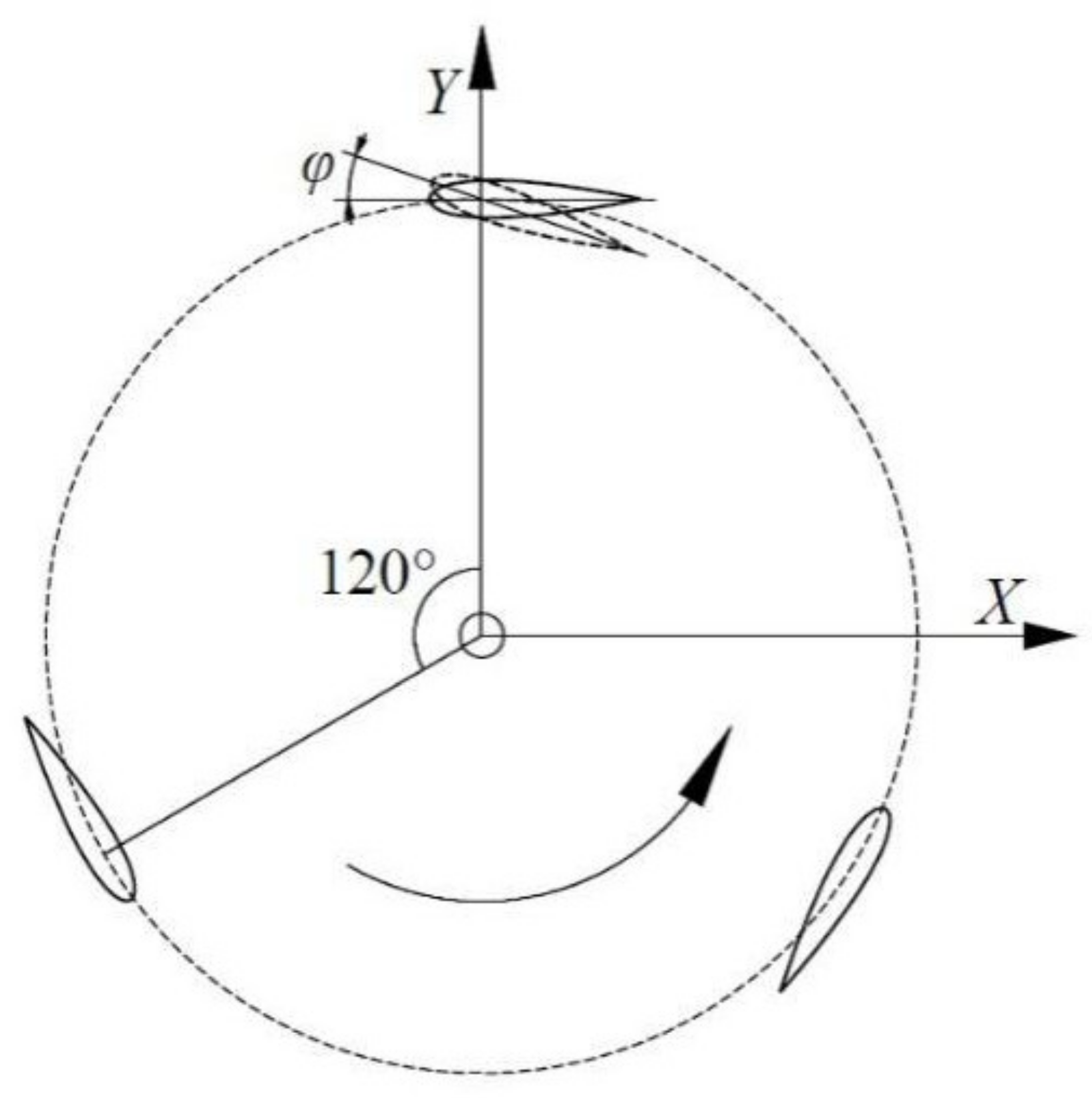
2.1. Selection and Parameters
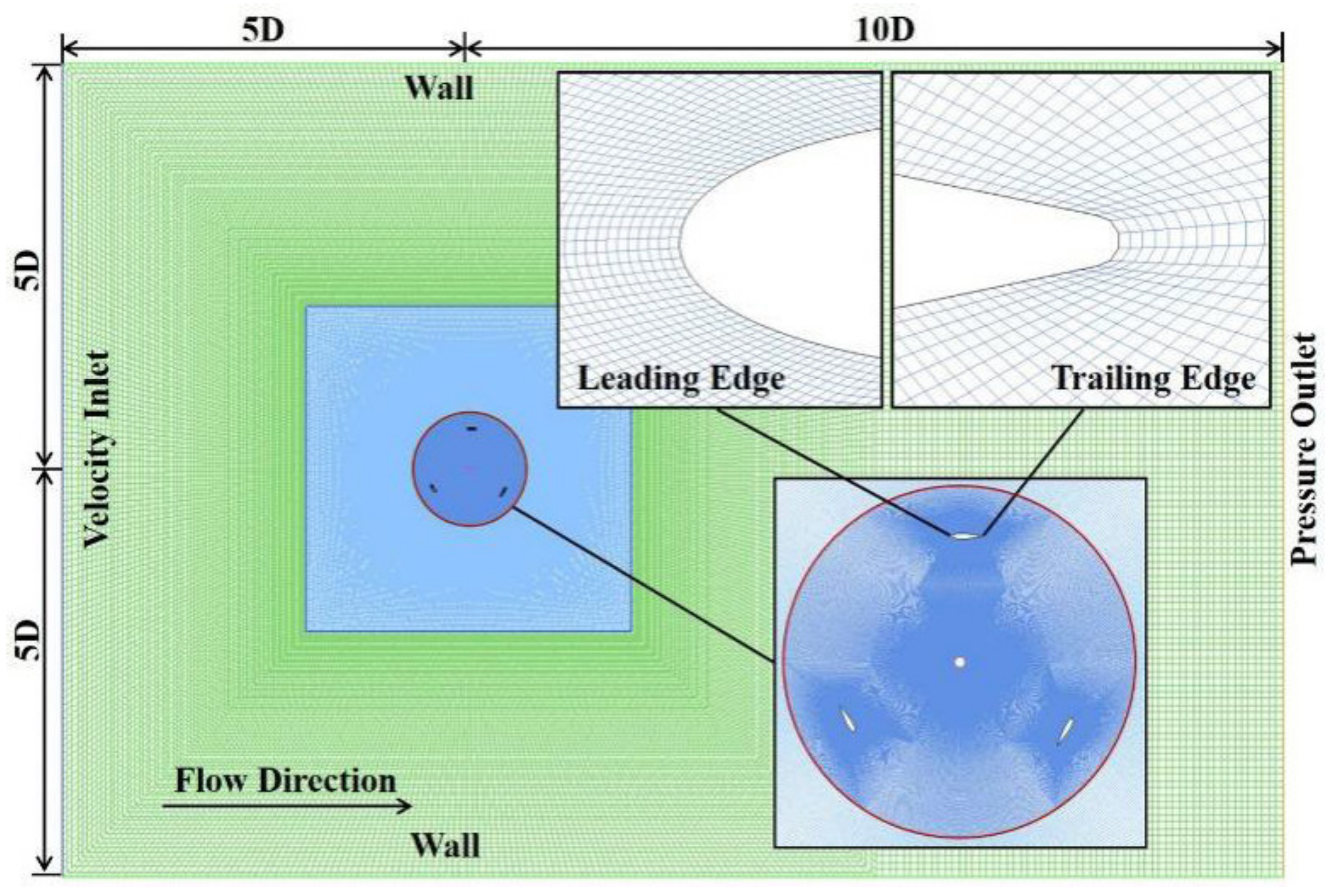
2.2. Computational Domain and Grid
2.3. Solver and Turbulence Model
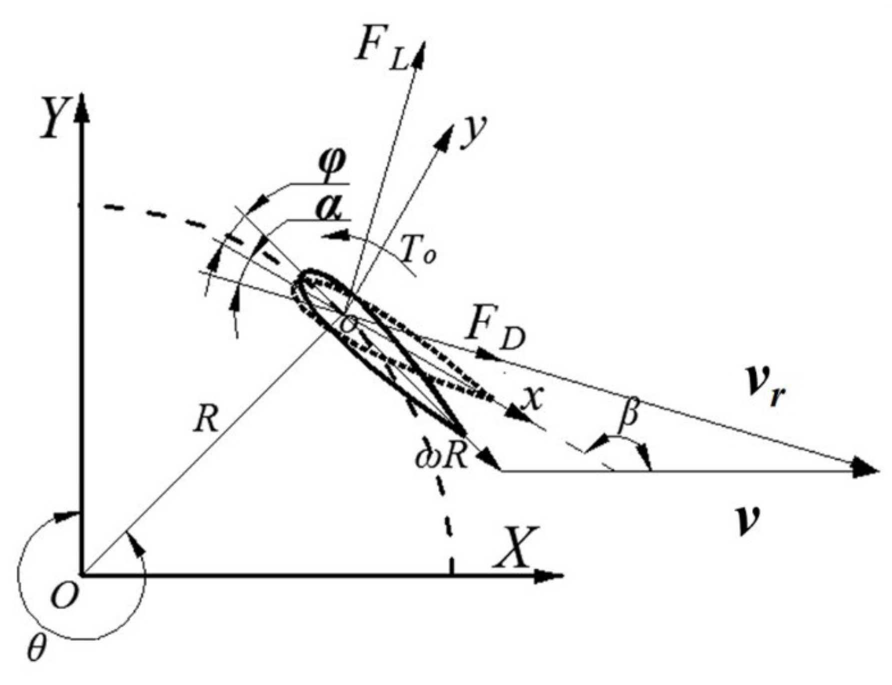
2.4. Rotor Dynamics and Dimensionless Parameters
2.5. Mesh and Time Step Selection
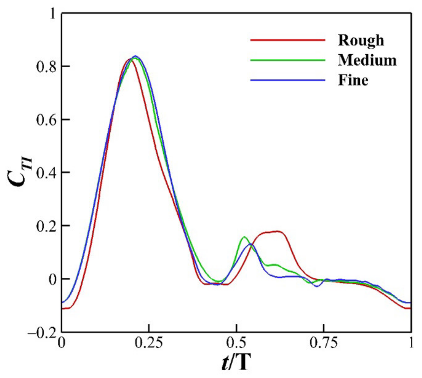
2.5.1. Mesh Convergence Study
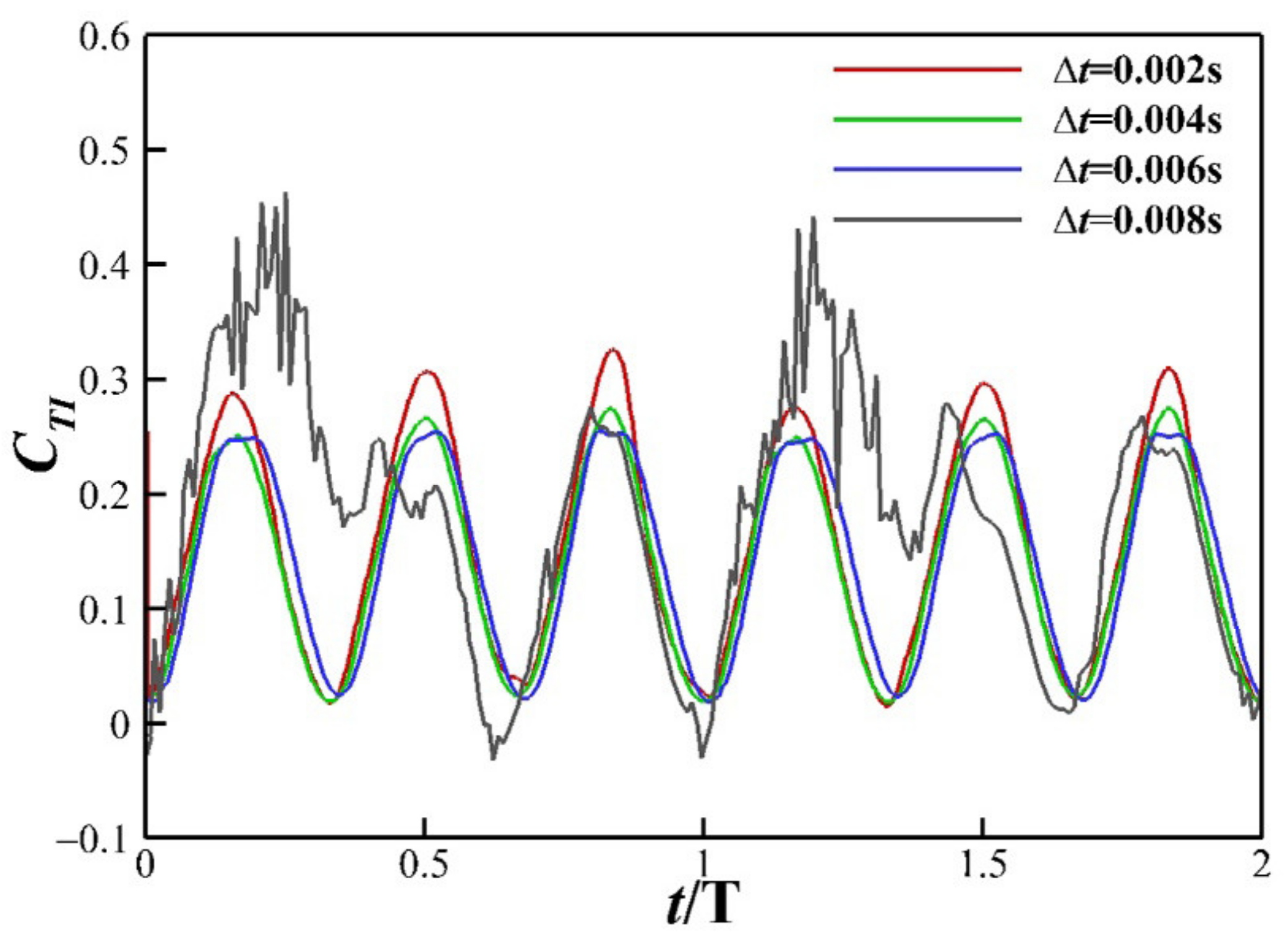
2.5.2. Time Convergence Study
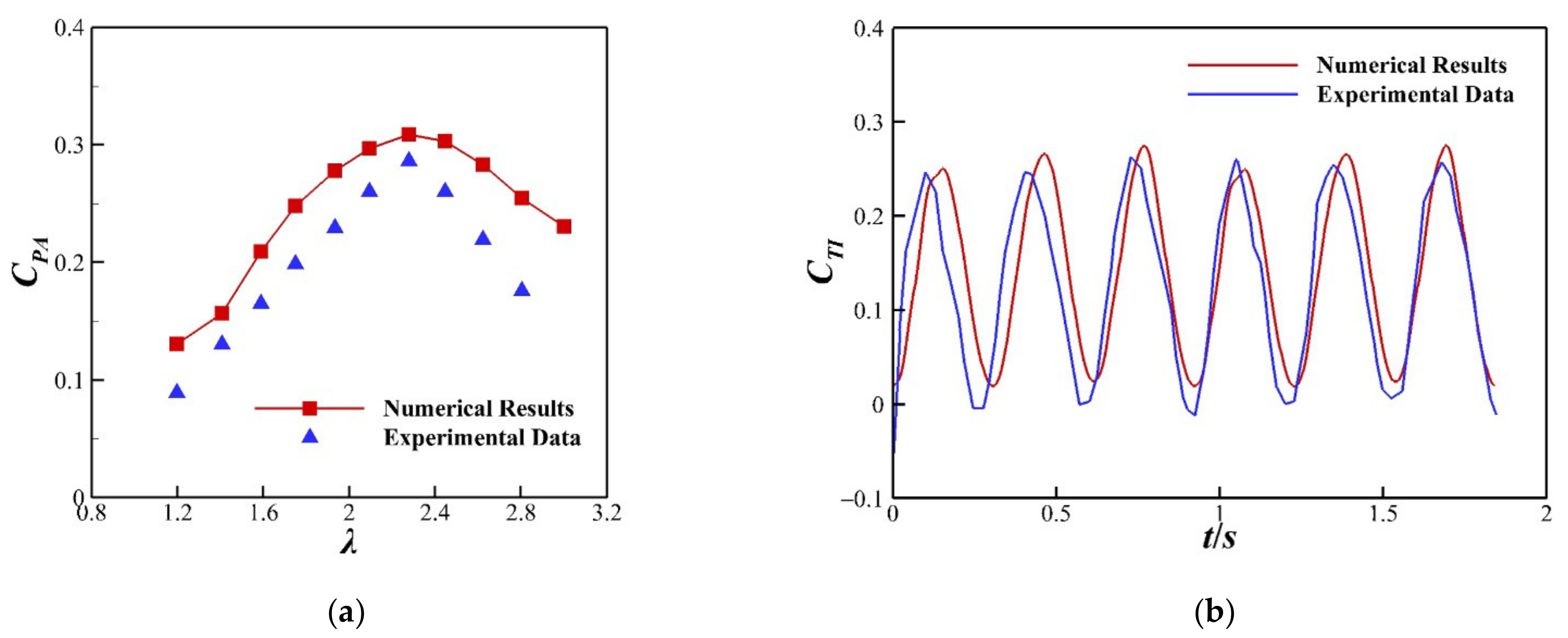
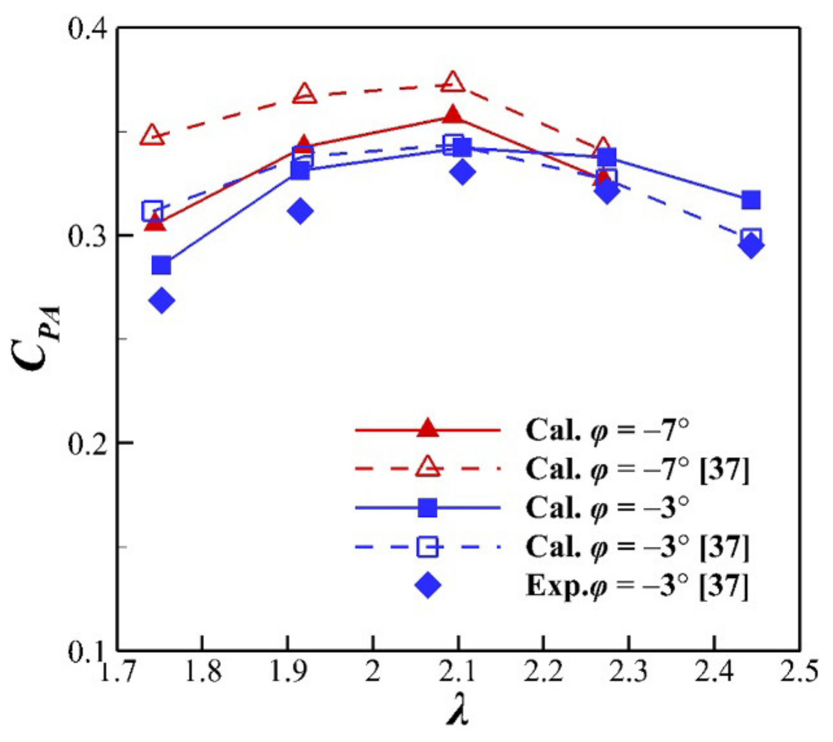
3. Numerical Model Validation
4. Results
4.1. Stand-Alone Turbine
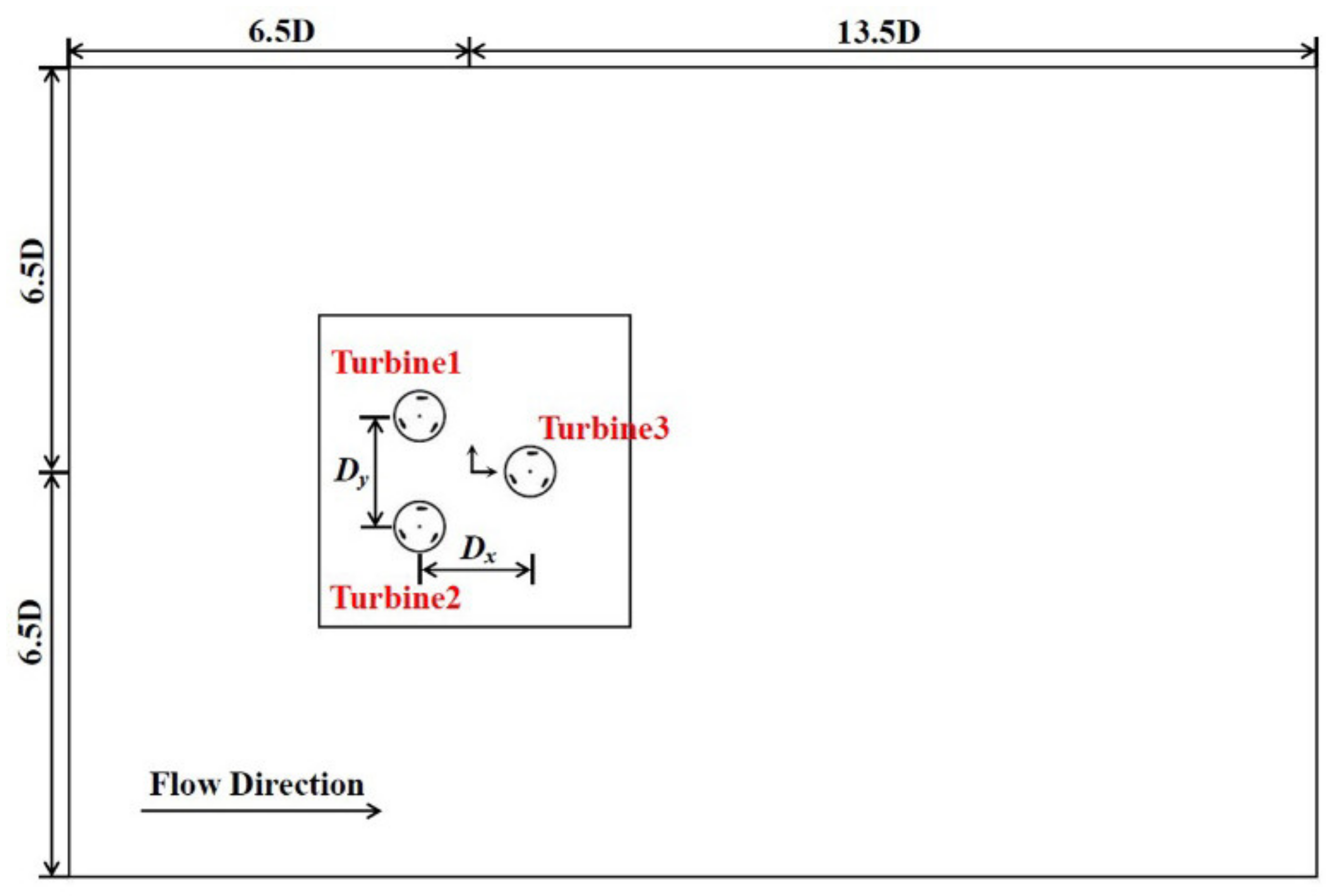
4.2. Double-Row Turbine Array
5. Conclusions
- (1)
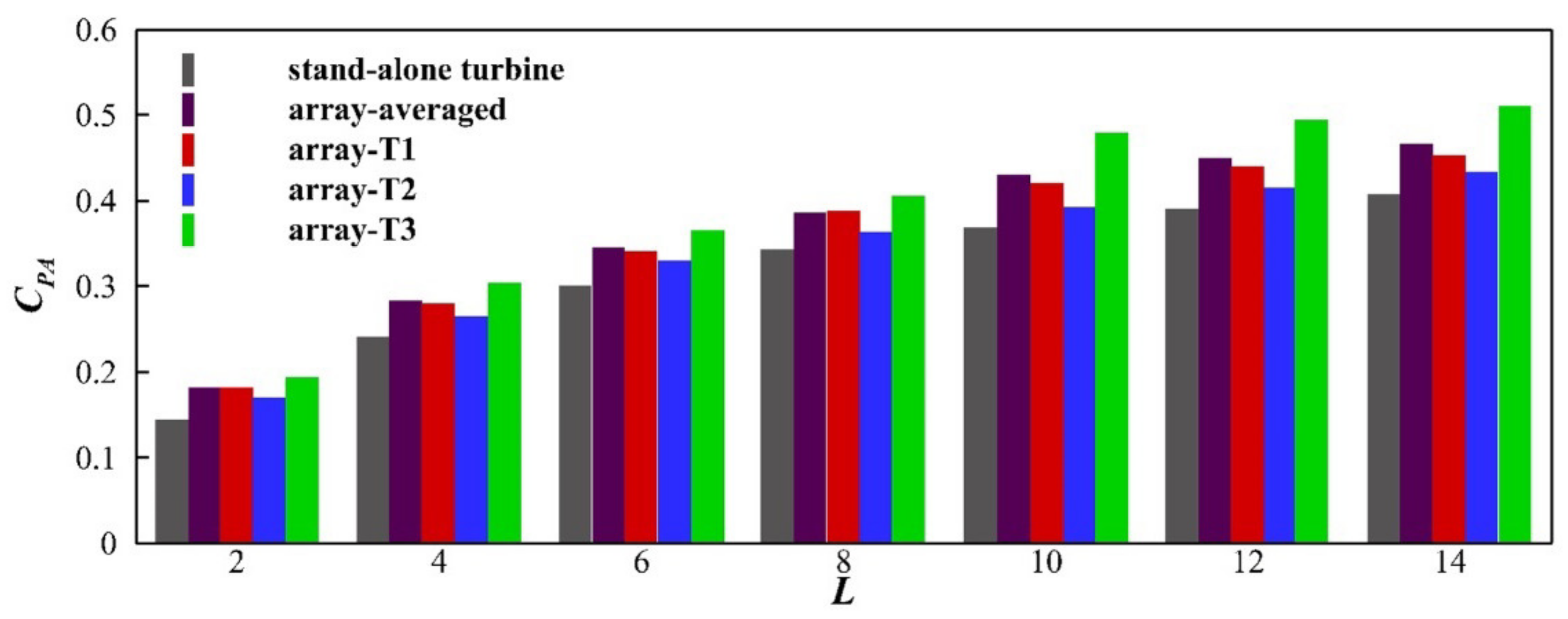
- Compared with a stand-alone turbine, the power coefficients of the three turbines in the array all improved, and as the load increased, the difference between the average power coefficients of the array and the stand-alone turbine became more obvious. When L = 2, the averaged power coefficient of three turbines in the array was 0.181, and the value was 0.010 higher than that of the stand-alone turbine. When L = 14, the average power coefficient of the three turbines in the array was 0.465, and this difference increased to 0.030.
- (2)
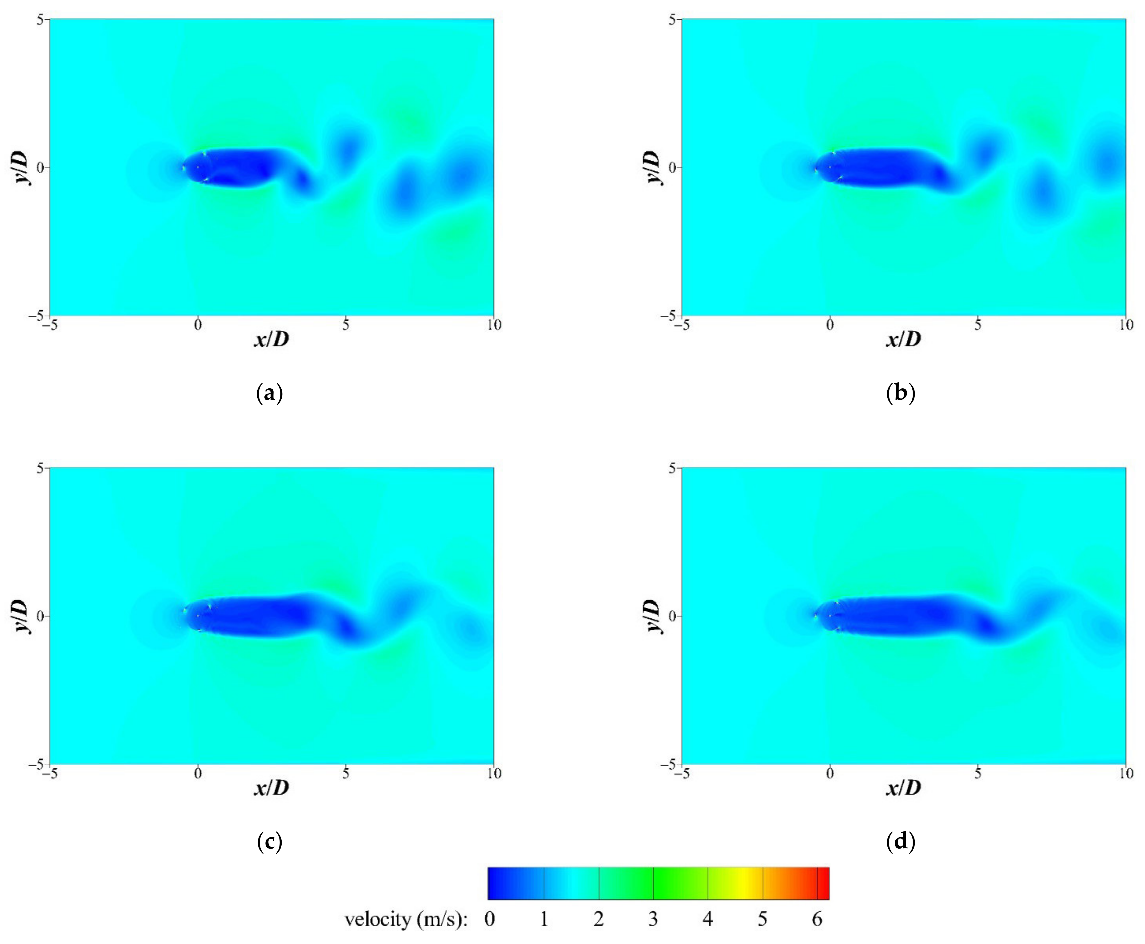
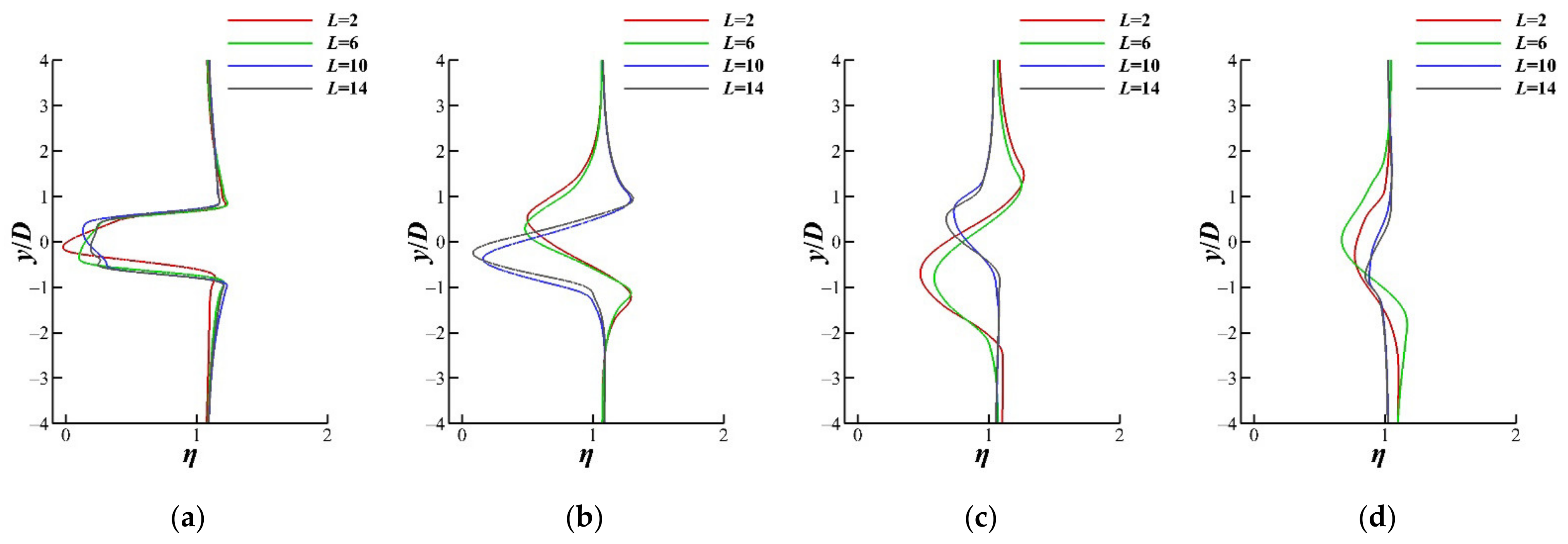
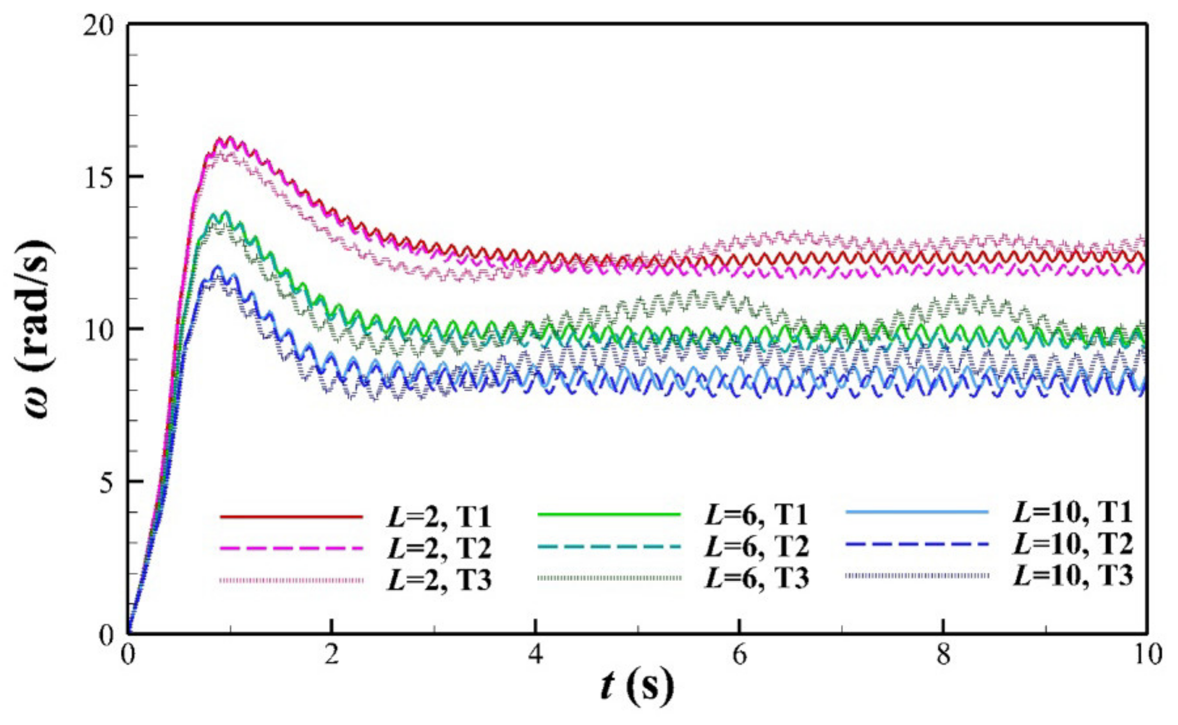
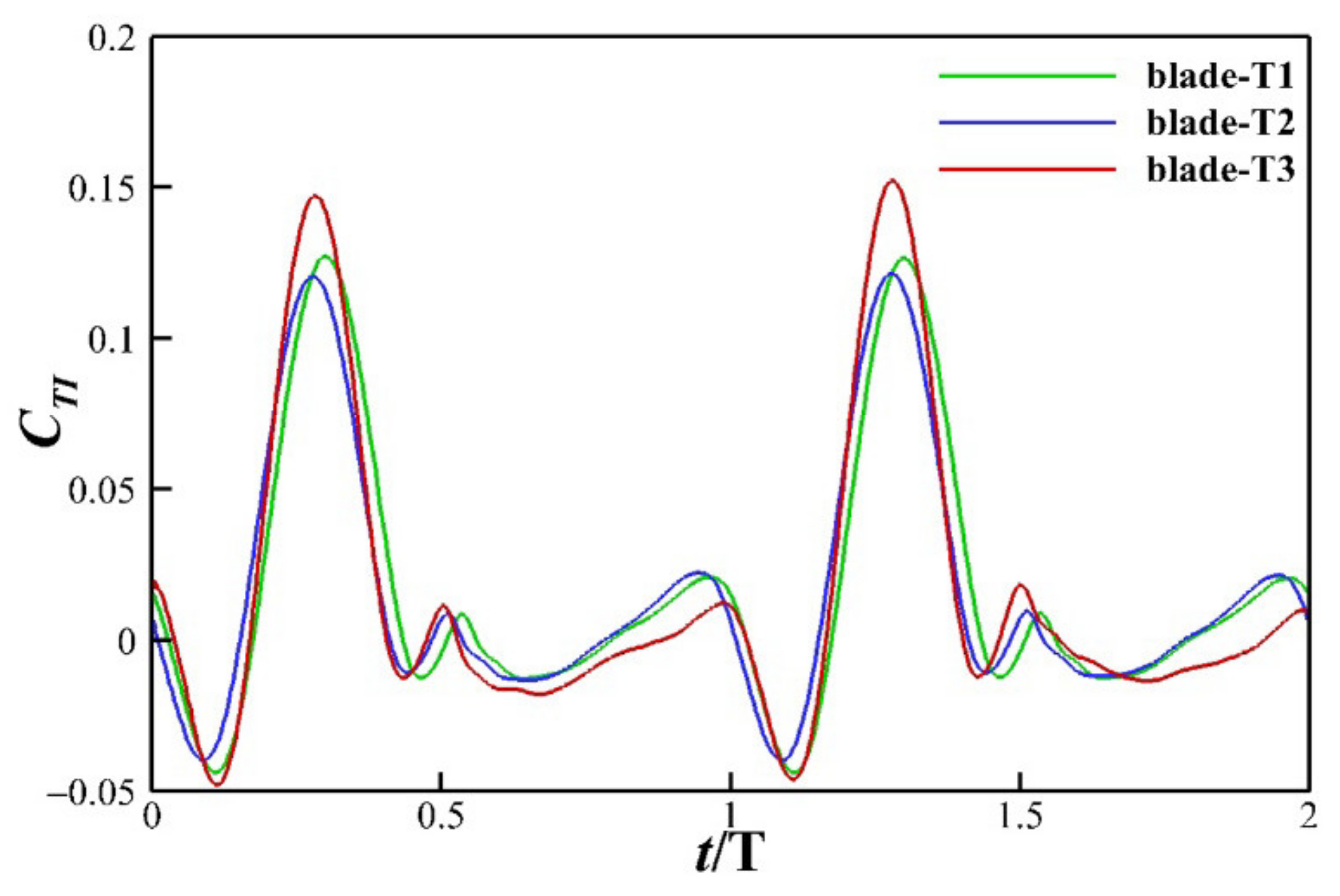
- In the array, the main effects of the front turbines T1 and T2 on the rear turbine T3 were energy utilization and turbine vibration. The fluid flow rate increased due to the beam effect between T1 and T2. The incident flow rate of T3 increased to approximately 1.2v, its rotational speed of T3 accelerated, and its power efficiency was enhanced. The superposition of the front turbine wake and other factors caused the velocity deficit area behind T3 to be larger, and the increase in the incident velocity made the force difference between the first and second half-cycles larger, resulting in greater rotational fluctuations in T3, meaning that although T3 had higher power coefficients, it was more susceptible to fatigue damage. There was little difference in the self-starting times between the three turbines. The rear turbine could affect the wake development and thus the performance of the front turbine, so there was a slight difference in performance between T1 and T2 despite using the same incident flow.
- (3)
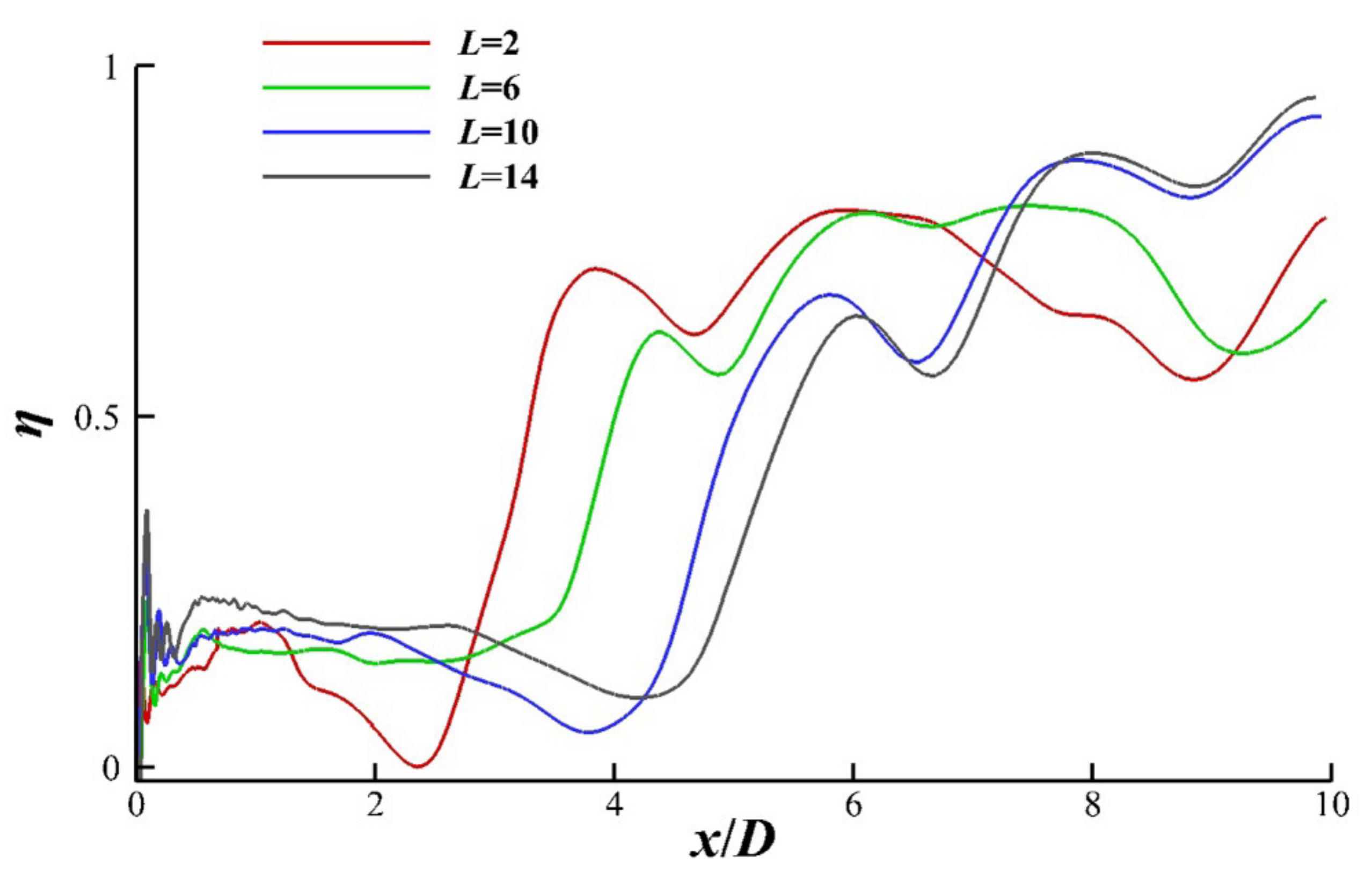
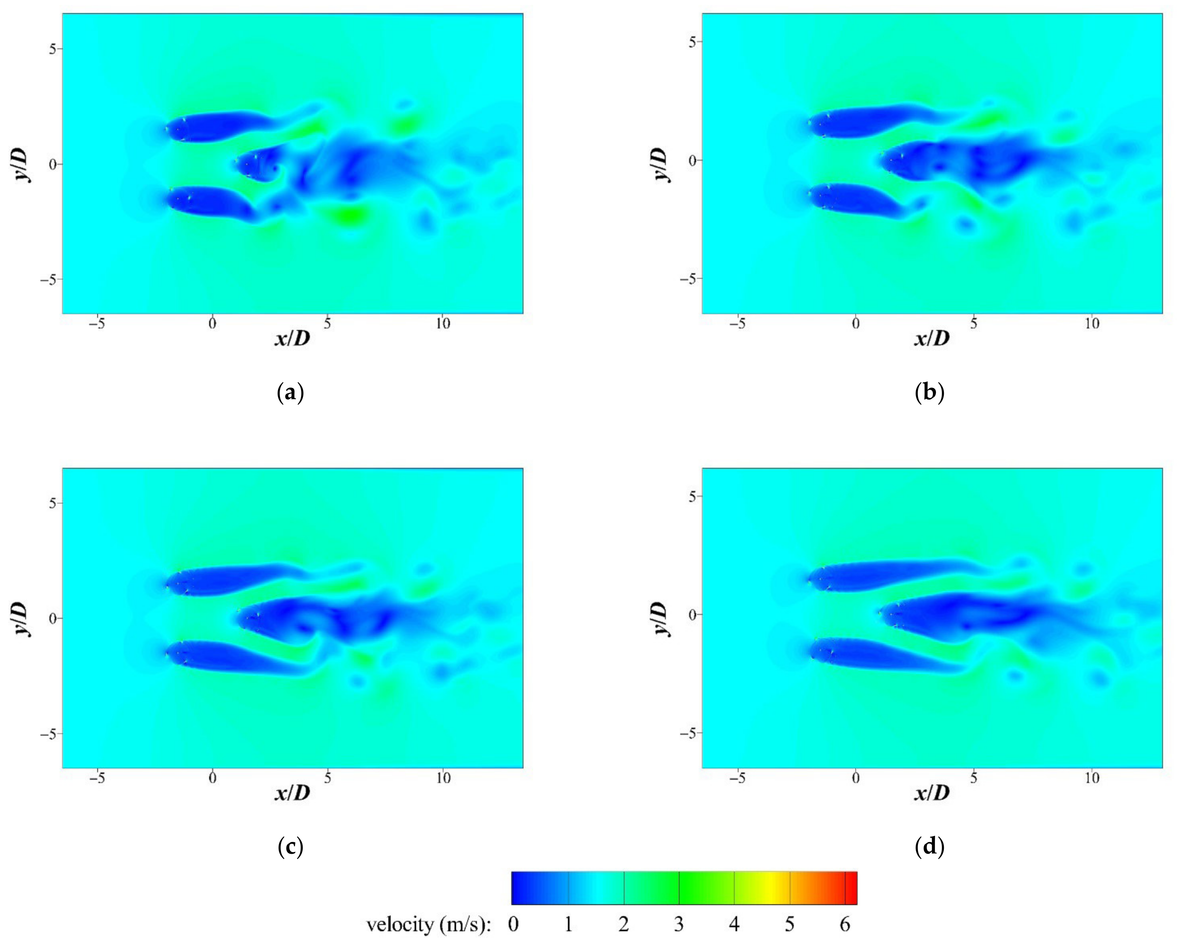
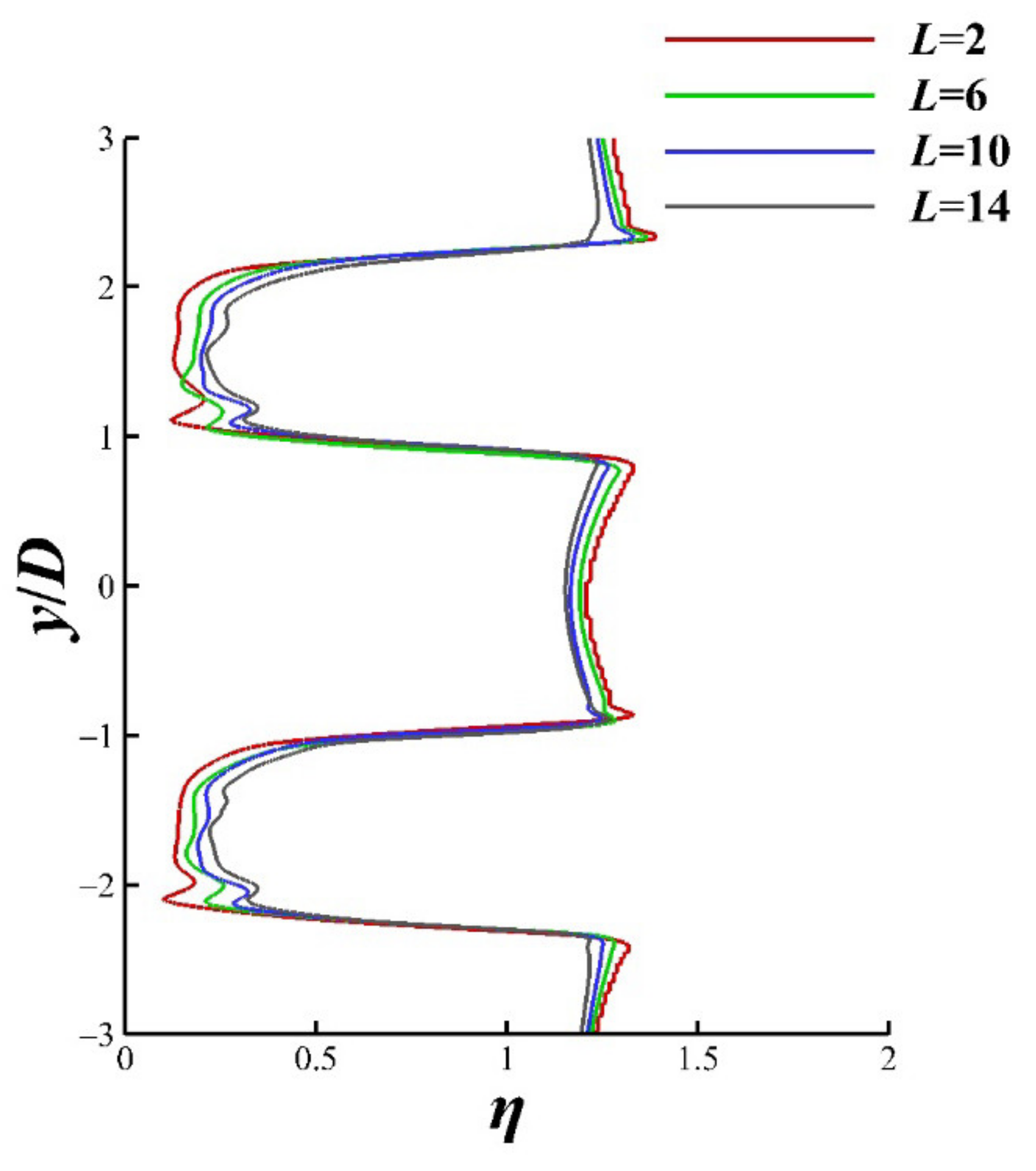
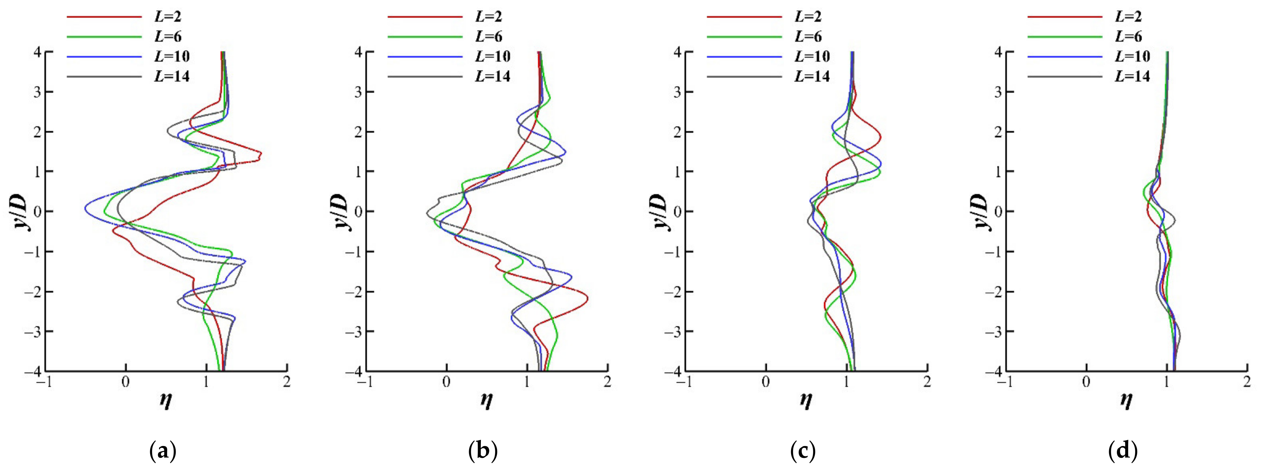
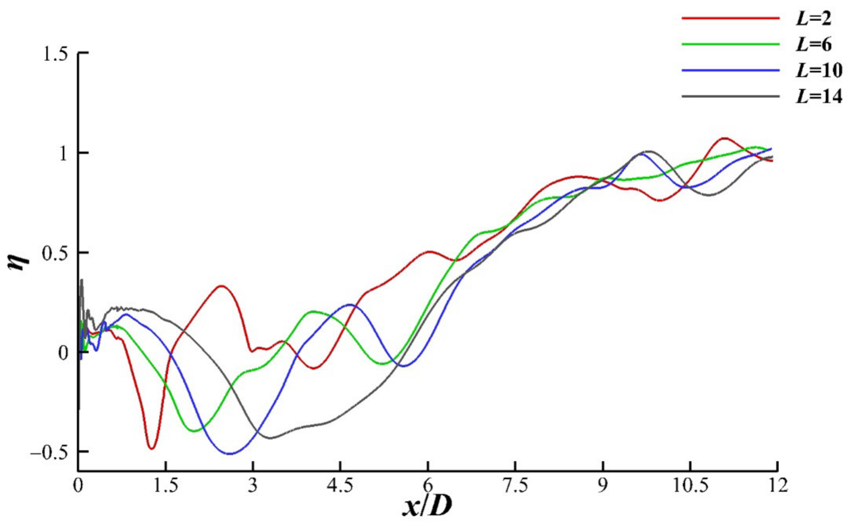
- In the array, the wake behind T3 had a much larger area of influence and more intense turbulence, with a greater velocity deficit than for the stand-alone turbine at the same load, but it recovered more quickly, with the wake recovering to over 95% at a distance of 10D behind it. For a stand-alone self-starting turbine, the rate of wake velocity recovery is load-dependent, but this was not evident in the arrays. In practice, axial and radial spacings of 3D are reasonable for a double-row turbine array.
- (4)
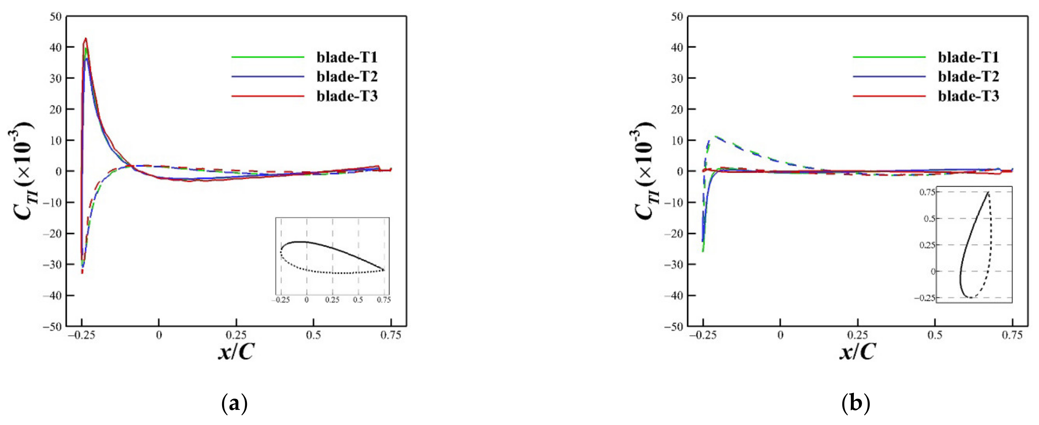
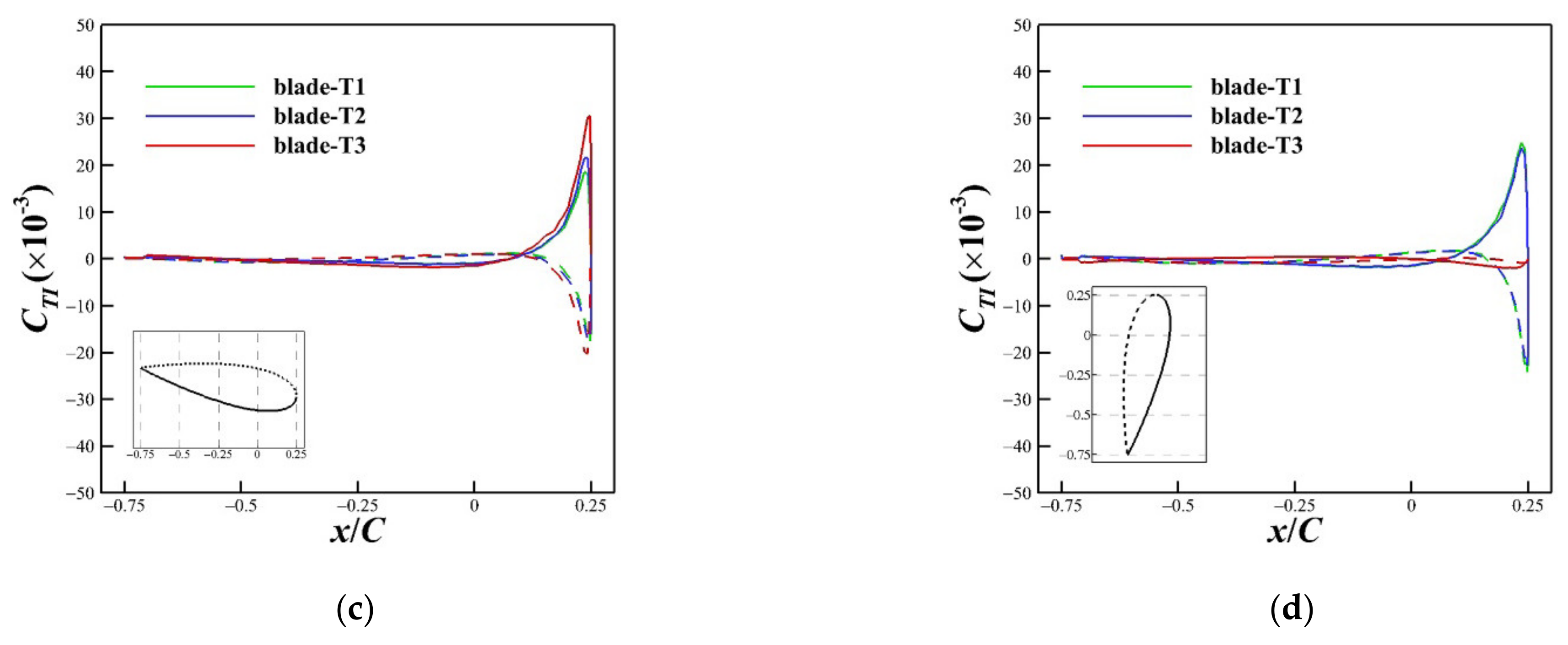
- The positive torque of the turbine was mainly generated when the blade rotated through the azimuth angle of 45–160° and mainly benefited from the inner side of the blade.
Author Contributions
Funding
Conflicts of Interest
References
- Hou, J.; Zhu, X.; Liu, P. Current situation and future projection of marine renewable energy in China. Int. J. Energy Res. 2019, 43, 662–680. [Google Scholar] [CrossRef]
- Li, Y.; Liu, H.; Lin, Y.; Li, W.; Gu, Y. Design and test of a 600-kW horizontal-axis tidal current turbine. Energy 2019, 182, 177–186. [Google Scholar] [CrossRef]
- Liu, Y.; Ma, C.; Jiang, B. Development and the environmental impact analysis of tidal current energy turbines in China. In IOP Conference Series: Earth and Environmental Science; IOP Publishing: Bristol, UK, 2018. [Google Scholar]
- Roberts, A.; Thomas, B.; Sewell, P.; Khan, Z.; Balmain, S.; Gillman, J. Current tidal power technologies and their suitability for applications in coastal and marine areas. J. Mar. Sci. Eng. 2016, 2, 227–245. [Google Scholar] [CrossRef]
- Kirke, B.; Lazauskas, L. Limitations of fixed pitch Darrieus hydrokinetic turbines and the challenge of variable pitch. Renew. Energy 2011, 36, 893–897. [Google Scholar] [CrossRef]
- Khan, M.J.; Bhuyan, G.; Iqbal, M.T.; Quaicoe, J.E. Hydrokinetic energy conversion systems and assessment of horizontal and vertical axis turbines for river and tidal applications: A technology status review. Appl. Energy 2009, 86, 1823–1835. [Google Scholar] [CrossRef]
- Lee, J.; Kim, Y.; Khosronejad, A.; Kang, S. Experimental study of the wake characteristics of an axial flow hydrokinetic turbine at different tip speed ratios. Ocean Eng. 2020, 196, 106777. [Google Scholar] [CrossRef]
- Ouro, P.; Runge, S.; Luo, Q.; Stoesser, T. Three-dimensionality of the wake recovery behind a vertical axis turbine. Renew. Energy 2019, 133, 1066–1077. [Google Scholar] [CrossRef]
- Gipe, P.; Möllerström, E. An overview of the history of wind turbine development: Part I—The early wind turbines until the 1960s. Wind Eng. 2022; online first. [Google Scholar] [CrossRef]
- Bos, R. Self-Starting of a Small Urban Darrieus Rotor: Strategies to Boost Performance in Low-Reynolds-Number Flows. Master’s Thesis, Delft University of Technology, Delft, The Netherlands, 2012. [Google Scholar]
- Ebert, P.; Wood, D.H. Observations of the starting behaviour of a small horizontalaxis wind turbine. Renew. Energy 1997, 12, 245–257. [Google Scholar] [CrossRef]
- Celik, Y.; Ma, L.; Ingham, D.; Pourkashanian, M. Aerodynamic investigation of the start-up process of H-type vertical axis wind turbines using CFD. J. Wind Eng. Ind. Aerodyn. 2020, 204, 104252. [Google Scholar] [CrossRef]
- Mohamed, O.S.; Elbaz, A.; Bianchini, A. A better insight on physics involved in the self-starting of a straight-blade Darrieus wind turbine by means of two-dimensional Computational Fluid Dynamics. J. Wind Eng. Ind. Aerodyn. 2021, 218, 104793. [Google Scholar] [CrossRef]
- Tsai, H.C.; Colonius, T. Numerical Investigation of Capability of Self-Starting and Self-Rotating of a Vertical Axis Wind Turbine. In Proceedings of the APS Division of Fluid Dynamics Meeting Abstracts, Boston, MA, USA, 22–24 November 2015. [Google Scholar]
- Arab, A.; Javadi, M.; Anbarsooz, M.; Moghiman, M. A numerical study on the aerodynamic performance and the self-starting characteristics of a Darrieus wind turbine considering its moment of inertia. Renew. Energy 2017, 107, 298–311. [Google Scholar] [CrossRef]
- Sun, X.; Zhu, J.; Hanif, A.; Li, Z.; Sun, G. Effects of blade shape and its corresponding moment of inertia on self-starting and power extraction performance of the novel bowl-shaped floating straight-bladed vertical axis wind turbine. Sustain. Energy Technol. Assess. 2020, 38, 100648. [Google Scholar] [CrossRef]
- Sun, X.; Zhu, J.; Li, Z.; Sun, G. Rotation improvement of vertical axis wind turbine by offsetting pitching angles and changing blade numbers. Energy 2021, 215, 119177. [Google Scholar] [CrossRef]
- Calautit, K.; Aquino, A.; Calautit, J.K.; Nejat, P.; Jomehzadeh, F.; Hughes, B.R. A review of numerical modelling of multi-scale wind turbines and their environment. Computation 2018, 6, 24. [Google Scholar] [CrossRef]
- Ma, Y.; Hu, C.; Li, Y.; Li, L.; Deng, R.; Jiang, D. Hydrodynamic performance analysis of the vertical axis twin-rotor tidal current turbine. Water 2018, 10, 1694. [Google Scholar] [CrossRef]
- Satrio, D.; Utama, I. Numerical investigation of contra rotating vertical-axis tidal-current turbine. J. Mar. Sci. Technol. 2018, 17, 208–215. [Google Scholar] [CrossRef]
- Sun, K.; Ji, R.; Zhang, J.; Li, Y.; Wang, B. Investigations on the hydrodynamic interference of the multi-rotor vertical axis tidal current turbine. Renew. Energy 2021, 169, 752–764. [Google Scholar] [CrossRef]
- Ji, R.; Sun, K.; Wang, S.; Li, Y.; Zhang, L. Analysis of hydrodynamic characteristics of ocean ship two-unit vertical axis tidal current turbines with different arrangements. J. Coast. Res. 2018, 83, 98–108. [Google Scholar] [CrossRef]
- Khalid, S.S.; Shehzad, K.; Ali, N.; Zhang, L. To investigate hydrodynamic interaction between twin vertical axis turbine working side by side using CFX. In Proceedings of the 2017 14th International Bhurban Conference on Applied Sciences and Technology (IBCAST), Ialamabad, Pakistan, 10–14 January 2017. [Google Scholar]
- Li, Z.C.; Sheng, Q.H.; Zhang, L.; Cong, Z.M.; Jiang, J. Numerical simulation of blade-wake interaction of vertical axis tidal turbine. Adv. Mater. Res. 2012, 346, 318–323. [Google Scholar] [CrossRef]
- Ouro, P.; Stoesser, T. Wake generated downstream of a vertical axis tidal turbine. In Proceedings of the 12th European Wave and Tidal Energy Conference, Cork, Ireland, 27 August–1 September 2017. [Google Scholar]
- Tian, L.; Song, Y.; Zhao, N.; Shen, W.; Zhu, C.; Wang, T. Effects of turbulence modelling in AD/RANS simulations of single wind & tidal turbine wakes and double wake interactions. Energy 2020, 208, 118440. [Google Scholar]
- Birjandi, A.H.; Bibeau, E.L. Frequency analysis of the power output for a vertical axis marine turbine operating in the wake. Ocean Eng. 2016, 127, 325–334. [Google Scholar] [CrossRef]
- Sébastien, B.; Olivier, G.T.; Guy, D. Hydrokinetic turbine array modeling for performance analysis and deployment optimization 1. Trans. Can. Soc. Mech. Eng. 2018, 42, 1–12. [Google Scholar]
- Tremblay, O.G.; Dumas, G. A numerical study on the interaction between two cross-flow turbines in tandem configuration to support a simplified turbine model approach. J. Renew. Sustain. Energy 2020, 12, 054502. [Google Scholar] [CrossRef]
- Gauvin-Tremblay, O.; Dumas, G. Hydrokinetic turbine array analysis and optimization integrating blockage effects and turbine-wake interactions. Renew. Energy 2022, 181, 851–869. [Google Scholar] [CrossRef]
- Chen, B.; Su, S.; Viola, I.M.; Greated, C.A. Numerical investigation of vertical-axis tidal turbines with sinusoidal pitching blades. Ocean Eng. 2018, 155, 75–87. [Google Scholar] [CrossRef]
- Chen, B.; Nagata, S.; Murakami, T.; Ning, D. Improvement of sinusoidal pitch for vertical-axis hydrokinetic turbines and influence of rotational inertia. Ocean Eng. 2019, 179, 273–284. [Google Scholar] [CrossRef]
- Satrio, D.; Utama, I. Experimental investigation into the improvement of self-starting capability of vertical-axis tidal current turbine. Energy Rep. 2021, 7, 4587–4594. [Google Scholar] [CrossRef]
- Saini, G.; Saini, R.P. Comparative investigations for performance and self-starting characteristics of hybrid and single Darrieus hydrokinetic turbine. Energy Rep. 2020, 6, 96–100. [Google Scholar] [CrossRef]
- Asr, M.T.; Nezhad, E.Z.; Mustapha, F.; Wiriadidjaja, S. Study on start-up characteristics of H-Darrieus vertical axis wind turbines comprising NACA 4-digit series blade airfoils. Energy 2016, 112, 528–537. [Google Scholar] [CrossRef]
- Song, C.; Wu, G.; Zhu, W.; Zhang, X. Study on Aerodynamic Characteristics of Darrieus Vertical Axis Wind Turbines with Different Airfoil Maximum Thicknesses Through Computational Fluid Dynamics. Arab. J. Sci. Eng. 2020, 45, 689–698. [Google Scholar] [CrossRef]
- Guang, Z.; Yang, R.; Yan, L.; Zhao, P. Hydrodynamic performance of a vertical-axis tidal-current turbine with different preset angles of attack. J. Hydrodyn. B 2013, 25, 280–287. [Google Scholar]
- Wang, K.; Sun, K.; Sheng, Q.H.; Zhang, L.; Wang, S.Q. The effects of yawing motion with different frequencies on the hydrodynamic performance of floating vertical-axis tidal current turbines. Appl. Ocean Res. 2016, 59, 224–235. [Google Scholar] [CrossRef]
- Guo, F. Performance Analysis of Vertical-Axis Tidal Current Turbines and Optimizing Turbines Array. M. Chinese. Master’s Thesis, Dalian University of Technology, Dalian, China, 2013. [Google Scholar]
- Yagmur, S.; Kose, F. Numerical evolution of unsteady wake characteristics of H-type Darrieus Hydrokinetic Turbine for a hydro farm arrangement. Appl. Ocean Res. 2021, 110, 102582. [Google Scholar] [CrossRef]
- Hornshøj-Møller, S.D.; Nielsen, P.D.; Forooghi, P.; Abkar, M. Quantifying structural uncertainties in Reynolds-averaged Navier–Stokes simulations of wind turbine wakes. Renew. Energy 2021, 164, 1550–1558. [Google Scholar] [CrossRef]


| Symbol | Description | Value |
|---|---|---|
| R | Rotor Radius | 0.5 m |
| D0 | Rotor Shaft Diameter | 0.04 m |
| S | Blade Span | 1.0 m |
| C | Blade Chord | 0.12 m |
| N | Number of Blades | 3 |
| σ, σ = NC/πD | Solidity | 0.1146 |
| I | Moment of Inertia | 7.0 kg·m2 |
| Mesh | Total Domain Mesh Quantity | Rotating Domain Mesh Quantity | Thickness of the Blade First Layer (×10−4 m) | Y+ |
|---|---|---|---|---|
| Rough | 50,018 | 28,329 | 3.5 | 18.2–44.6 |
| Medium | 93,715 | 58,230 | 0.8 | 2.79–5.11 |
| Fine | 313,258 | 225,258 | 0.3 | 0.75–1.71 |
| Parameter | Value | |||||||||
|---|---|---|---|---|---|---|---|---|---|---|
| λ | 1.1971 | 1.4073 | 1.5898 | 1.7503 | 1.9328 | 2.0932 | 2.2790 | 2.4463 | 2.6223 | 2.8038 |
| Numerical Results | 0.1307 | 0.1569 | 0.2092 | 0.2478 | 0.2779 | 0.2965 | 0.3088 | 0.3027 | 0.2830 | 0.2546 |
| Experimental Data | 0.0892 | 0.1300 | 0.1647 | 0.1981 | 0.2291 | 0.2600 | 0.2860 | 0.2600 | 0.2191 | 0.1758 |
| μ | 0.0415 | 0.0269 | 0.0445 | 0.0497 | 0.0488 | 0.0365 | 0.0228 | 0.0427 | 0.0639 | 0.0788 |
| 0.0456 | ||||||||||
| Parameter | Value | ||||||
|---|---|---|---|---|---|---|---|
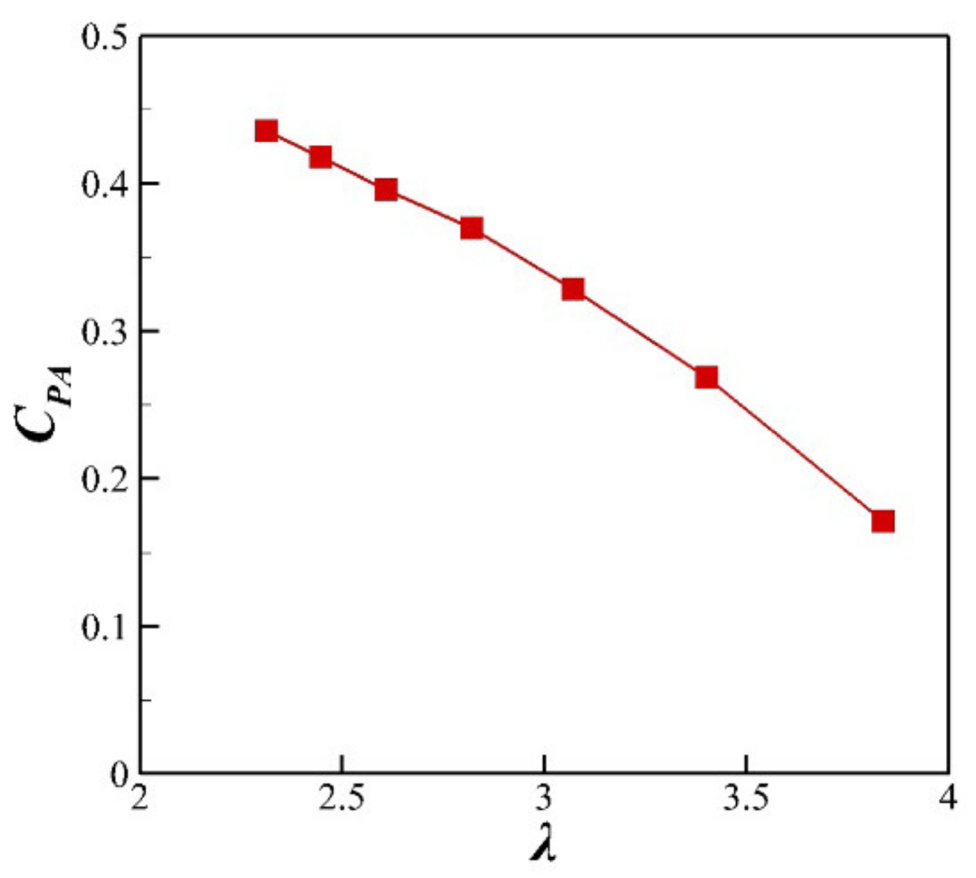
| L | 14 | 12 | 10 | 8 | 6 | 4 | 2 |
| λ | 2.313 | 2.448 | 2.611 | 2.822 | 3.071 | 3.403 | 3.838 |
| CPA | 0.435 | 0.418 | 0.396 | 0.370 | 0.328 | 0.269 | 0.171 |
Publisher’s Note: MDPI stays neutral with regard to jurisdictional claims in published maps and institutional affiliations. |
© 2022 by the authors. Licensee MDPI, Basel, Switzerland. This article is an open access article distributed under the terms and conditions of the Creative Commons Attribution (CC BY) license (https://creativecommons.org/licenses/by/4.0/).
Share and Cite
Zhu, L.; Hou, E.; Zhou, Q.; Wu, H. Numerical Experiments on Hydrodynamic Performance and the Wake of a Self-Starting Vertical Axis Tidal Turbine Array. J. Mar. Sci. Eng. 2022, 10, 1361. https://doi.org/10.3390/jmse10101361
Zhu L, Hou E, Zhou Q, Wu H. Numerical Experiments on Hydrodynamic Performance and the Wake of a Self-Starting Vertical Axis Tidal Turbine Array. Journal of Marine Science and Engineering. 2022; 10(10):1361. https://doi.org/10.3390/jmse10101361
Chicago/Turabian StyleZhu, Lining, Erhu Hou, Qingwei Zhou, and He Wu. 2022. "Numerical Experiments on Hydrodynamic Performance and the Wake of a Self-Starting Vertical Axis Tidal Turbine Array" Journal of Marine Science and Engineering 10, no. 10: 1361. https://doi.org/10.3390/jmse10101361
APA StyleZhu, L., Hou, E., Zhou, Q., & Wu, H. (2022). Numerical Experiments on Hydrodynamic Performance and the Wake of a Self-Starting Vertical Axis Tidal Turbine Array. Journal of Marine Science and Engineering, 10(10), 1361. https://doi.org/10.3390/jmse10101361