Article

Quantitative Evaluation of Submerged Cavitation Jet Performance Based on Image Processing Method

1
Marine Engineering College, Dalian Maritime University, Dalian 116026, China
2
College of Ocean Engineering, Guangdong Ocean University, Zhanjiang 524088, China
*
Author to whom correspondence should be addressed.
J. Mar. Sci. Eng. 2022, 10(10), 1336; https://doi.org/10.3390/jmse10101336
Submission received: 2 August 2022 / Revised: 5 September 2022 / Accepted: 15 September 2022 / Published: 20 September 2022
(This article belongs to the Section Marine Pollution)

Abstract

:
The submerged cavitation jet is suitable for ocean engineering activities such as ship fouling cleaning, organic wastewater treatment, offshore oil drilling, and natural gas hydrate extraction due to its superior hydraulic performance and erosion capacity. As an intuitive analysis method, image processing is widely used to investigate the characteristics of submerged cavitation jets. However, due to the lack of quantitative evaluation of the cavitation cloud in image processing, it is difficult to establish the relationship between cavitation cloud image and cavitation performance. Therefore, a novel image processing method based on dimensionless grayscale intensity is proposed in this paper. This method was used under different sample spaces to obtain the maximum mass loss of the sample. The results showed that the method could accurately calculate the maximum mass loss of the sample based on the image processing results. When the sample space is 200 images and the working pressure is 20 MPa, the calculation error of the image processing method for the maximum mass loss of the sample is 1.26%. For the sample spaces of 10–5000 images, the maximum calculation error of the image processing method for the maximum mass loss of the samples is 3.29%. The image processing method proposed in this paper establishes the relationship between the cavitation cloud image and the maximum mass loss of the samples, which provides help for further understanding and application of submerged cavitation jets.

1. Introduction

The submerged cavitation jet is widely used in ocean engineering due to its superior hydraulic performance and erosion capacity. Meeting the demand of environmental protection and energy saving, a submerged cavitation jet can be used directly by underwater robots or divers to clean ship fouling in order to reduce ship fuel consumption and the risk of biological invasion [1]. Hydrodynamic cavitation generates hydroxyl radicals, making it possible as a new advanced oxidation process [2]. This promotes the application of hydrodynamic cavitation in the field of wastewater treatment [3]. Currently, water pollution affects the marine ecological environment. Submerged cavitation jets could be a cheaper and cleaner way to treat organic wastewater, reducing ocean pollution [4]. Scale deposition in the wellbores of gas or oil wells leads to higher production and transportation costs, which can be alleviated by using cavitation jets to remove barium sulfate fouling in pipelines [5]. Moreover, benefiting from powerful cavitation erosion and impact force, the submerged cavitation jet is an effective rock-breaking method which is suitable for offshore oil drilling and exploitation [6]. In recent years, more natural gas hydrates have been found in the deep seabed, and the global seabed reserves of this resource are enormous [7]. As a powerful crushing method with a lighter mechanical structure which is relatively easy to carry on flexible pipes, the submerged cavitation jet offers tremendous advantages for exploiting natural gas hydrate deposits [8]. From cleaning ship fouling to rock breaking, oil drilling, and gas hydrate extraction, the submerged cavitation jet is suitable for ocean engineering due to its simple structure and superior performance. With the rise in the world’s ocean trade and in the development of ocean resources, the prospects for application of submerged cavitation jets will be increasingly broad in the future.
At present, there are four main methods for evaluating the performance of submerged cavitation jets: the sample erosion method [9,10,11,12], the image processing method [13,14], the noise detection method [15,16], and the pressure detection method [17,18]. Compared with the other three methods, the image processing method has the ability to generate intuitive image data and highlight detailed dynamic changes in the submerged cavitation jet. At the same time, unlike the sample erosion method, which is time-consuming and costly, the image processing method only involves acquiring images for a short time and can be used to perform analysis with almost no material consumption. An essential tool for the study of the submerged cavitation jet by the image processing method is a high-speed camera which can capture high frame rate images of the cavitation cloud, in order to explore the changing laws of the cavitation cloud and characterize the performance of the submerged cavitation jet. Due to the intuitiveness and convenience of visualization techniques, high-speed cameras have been increasingly adopted by researchers in recent years [19,20]. By adjusting the brightness of lights, the high-speed camera can filter the surrounding flow field and capture high frame rate images of the spatiotemporal distribution of the cavitation clouds [21]. The cavitation clouds in the submerged cavitation jet change periodically during inception, growth, shedding, and collapse [22]. The periodic variation law of the cavitation cloud determines that it has a specific shedding frequency [23]. The shedding frequency of the cavitation cloud reflects the changes in growth and collapse rate, which affect the number and state of cavitation bubbles, and ultimately lead to the differences in cavitation intensity at various stages. Cavitation clouds show a range of lengths, widths, and areas under different working conditions, reflecting the overall cavitation state at that time [24]. Unfortunately, the original images captured by high-speed camera can only reflect the overall intuitive state of the cavitation cloud, and cannot directly indicate the characteristic distribution of the flow field inside the cavitation cloud.
The image processing method is the most important means to analyze the characteristics of the submerged cavitation jet flow field. The core concept in image processing is the processing and quantification of the original image data to obtain clear and specific flow field characteristics. Wu et al. [25] studied the dynamic behavior of the Helmholtz self-excited oscillating jet using high-speed photography. Grayscale values were processed using various statistical methods to analyze the cavitation cloud generated by a Helmholtz self-sustained oscillation jet. They found that the length and period of the cavitation cloud generated by Helmholtz self-sustained oscillation jets are usually significantly influenced by changes in geometry and operating pressure. The frame difference method (FDM) is another widely used method for processing images of submerged cavitation jets at work. It is also an effective method for analyzing and evaluating the unsteady behavior of cavitation clouds [26,27]. The FDM can capture the growth and the shedding of the cavitation clouds, especially the change of the cavitation clouds on both sides of the shear layer [28,29]. However, it cannot be distinguished whether the growth and shedding of cavitation clouds is caused by the state or the movement of cavitation bubbles. This is an inevitable defect of the FDM itself. It is worth emphasizing that the quantization of grayscale intensity, which is often associated with the FDM, can be used for dimensionless processing of grayscale values. This quantization method processes raw grayscale values to generate a distribution of grayscale intensity which can directly reflect the collapse behavior of the cavitation cloud [30,31]. Peng et al. [32] analyzed the spatiotemporal distribution of cavitation cloud using Proper Orthogonal Decomposition (POD). They found that POD modes of side-view images could be used to evaluate the maximum radial distribution of cavitation pits. In the stable frequency zone where the cavitation cloud sheds, the weighting coefficients of the second mode of POD can be used to reliably calculate the shedding frequency of the cavitation cloud generated by the submerged cavitation jet [33]. The above image processing methods have promoted research on the mechanism and characteristics of submerged cavitation jets, and make an important contribution to research on the visualization of these tools at work. However, existing investigations of the visualization of submerged cavitation jets focus on the dynamic characteristics of the cavitation cloud, while the intensity of the overall cavitation cloud has not been adequately represented. Not only that, most of the existing image processing methods are based on qualitative evaluation, leaving a lack of quantitative evaluation of the submerged cavitation jet. In addition, visualization studies of cavitation clouds usually focus on the cavitation clouds themselves. The relationship between cavitation cloud images and the erosion capacity of the submerged cavitation jet has not yet been established, and requires further study.
In order to establish a quantitative evaluation mechanism for the image processing method, a novel approach based on dimensionless grayscale intensity is proposed in this paper. Based on the relationship between the cavitation cloud images and the erosion capacity, the maximum mass loss of the sample eroded by the submerged cavitation jet under different working pressures can be obtained directly through image processing. Therefore, an experimental setup was built to measure erosion caused by a submerged cavitation jet in order to establish the mass loss of the sample and observe the cavitation cloud images.

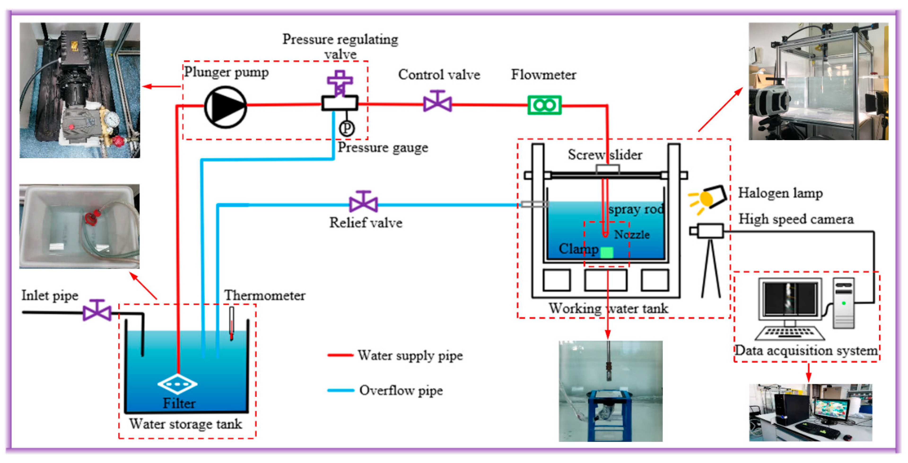
2. Experimental Setup and Methodology

2.1. Experimental Setup

The submerged cavitation jet experimental setup is shown in Figure 1. The experimental setup consists of five parts: the water supply pipeline, the working water tank, the overflow pipeline, the water storage tank, and the image capturing system. In the water supply pipeline, an experimental nozzle, a spray rod, a turbine flowmeter, a control valve, a pressure-regulating valve, a plunger pump, and a filter were arranged in order. The submerged cavitation jet generator in the experiment was an organ pipe nozzle [34]. The schematic diagram and the experimental nozzle dimensions are shown in Figure 2 and Table 1, respectively. A turbine flowmeter with a precision grade of 0.5 was used to monitor the flow of the water supply pipeline in real-time. The control valve controlled the opening and closing of the water supply pipeline. A pressure-regulating valve with a range of 0–40 MPa and a precision grade of 1.5 was used to adjust the working pressure to 0–20 MPa. The maximum pressure of the supply water provided by the plunger pump was 20 MPa and the maximum flowrate was 10 L/min. A standard mesh 140 filter was used to prevent impurities from entering the pipeline.
In the working water tank, a clamp for fixing the target was installed on the bottom, and a screw slider device for controlling the X, Y, and Z axis movement of the spray rod was installed on the top. The experimental nozzle was installed at the lower end of the spray rod. The clamp was directly beneath the experimental nozzle. The overflow pipeline was arranged in the pressure-regulating valve and the working water tank. The overflow pipeline connected to the pressure-regulating valve was used to discharge the supply water to the storage water tank to change the working pressure of the experimental nozzle. Another overflow pipeline connected to the working water tank kept the water level in the working water tank constant, so as to keep the confining pressure on experimental nozzle constant during the experiment. The water storage tank was used to replenish fresh water and store overflow water. The water temperature had little influence on the experiment results. A thermometer was placed in the water storage tank to monitor the water temperature in real-time. In order to keep the initial water temperature of each experiment constant, the water in both tanks had to be replaced before each experiment. The initial temperature of all experiments was 12 °C. The image capturing system included a high-speed camera, a data acquisition system, and two halogen lamps. The high-speed camera (Phantom V2012, manufactured by AMETEK in Edison, NJ, USA) was used to capture continuous high frame rate images of the cavitation cloud. The size of the shooting area was set to 256 × 256 pixels, the shooting frame rate was set to 20,000 fps, and the exposure time was set to 25 μs. The output resolution of all images was 96 dpi. The data acquisition system was used to obtain and preprocess all cavitation cloud images taken by the high-speed cameras. Two halogen lamps were placed on either side of the working water tank to illuminate experiment zone. Both lamps were kept at the same brightness.

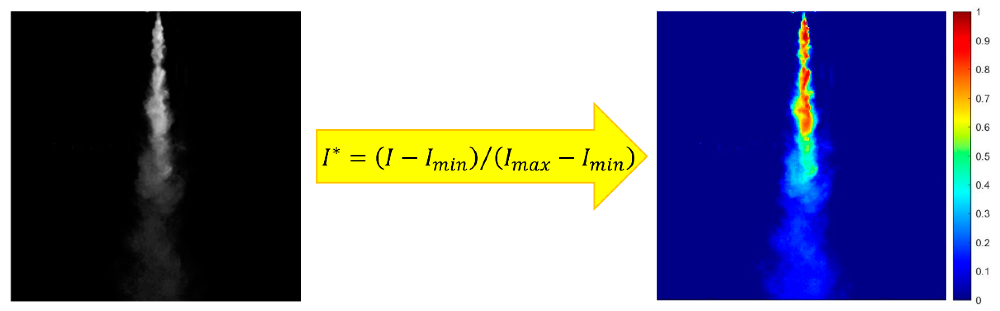
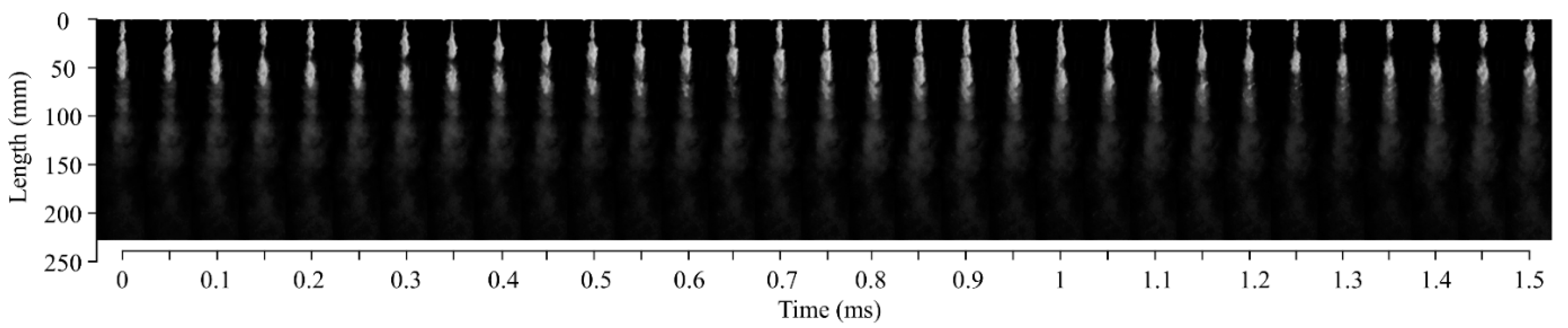
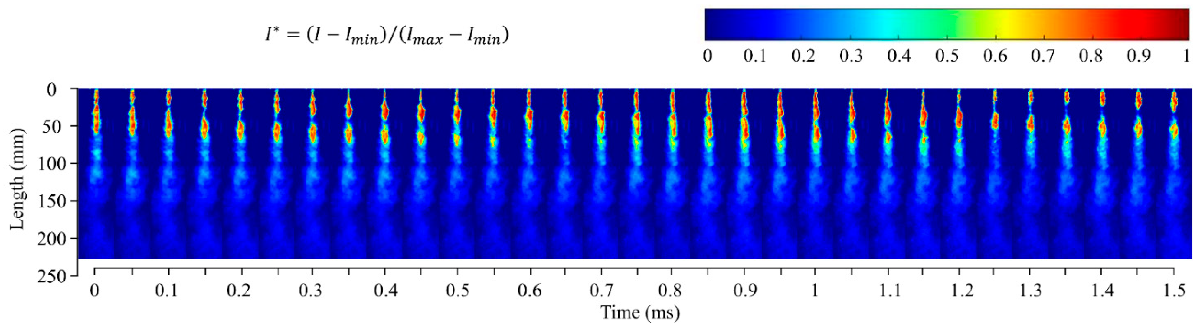
2.2. Image Processing Method

The light transmission of vapor bubbles is much lower than that of water. When the light from the halogen lamp was projected onto the vapor–liquid interface of the cavitation bubbles, the cavitation bubbles reflected part of the light into the camera lens. The cavitation cloud in the image appeared white. The higher the density of the cavitation bubble, the higher the brightness of the image obtained by the camera. After the images were converted to grayscale, each pixel corresponded to a certain grayscale value that was proportional to the brightness of the image. Therefore, the larger the grayscale value, the higher the density of the cavitation bubbles. The density of the cavitation bubbles reflects the cavitation intensity produced by the submerged cavitation jet. The dimensionless grayscale intensity value, which represents the density of the cavitation bubbles, can be obtained by means of dimensionless processing of the grayscale values, as shown in Equation (1) [35].
I * = ( I I m i n ) / ( I m a x I m i n )
where I * is the dimensionless grayscale intensity of each pixel, I is the grayscale value of each pixel, I m i n is the minimum grayscale value of all regions of the image, and I m a x is the maximum grayscale value of all regions of the image.
Figure 3 shows the dimensionless grayscale intensity distribution of the cavitation cloud image after the image processing described above. In the figure, red represents regions with a higher density of cavitation bubbles, and blue represents regions with a lower density of cavitation bubbles. It can be seen that the density of cavitation bubbles in the core region of the cavitation cloud is higher, while the density of the cavitation bubbles in at edge is lower. It is generally known that the number of cavitation bubbles is the critical factor affecting the erosion capacity of a submerged cavitation jet. If surface integral analysis is performed on the grayscale distribution of the cavitation image, the dimensionless number of cavitation bubbles of the submerged cavitation jet can be obtained, as shown in Equation (2).
Q = 0 s 1 I * d s
where Q is the dimensionless number of cavitation bubbles and s 1 is the area of the cavitation image.
Since the calculated area of the cavitation image is a rectangular area, the surface integral can be easily converted into a double finite integral, as shown in Equation (3).
0 s 1 I * d s = 0 y 1 0 x 1 I * d x d y
where x 1 is the width of the cavitation image and y 1 is the height of the cavitation image.
The dimensionless grayscale intensity obtained by dimensionless processing is not a continuous function of the image, and cannot be integrated directly. In addition, the image itself is made up of a matrix of pixels. Therefore, the discrete method was used to perform double finite integration on the entire image, as shown in Equation (4).
0 y 1 0 x 1 I * d x d y = ω μ 0 n 0 m I i j *
where I i j * represents the grayscale intensity on the pixel coordinates (i, j) of the image, m represents the number of pixels in the horizontal direction, n represents the number of pixels in the vertical direction, and ω and μ represent the horizontal length and vertical height of each pixel, respectively.
Based on Equations (2)–(4), the dimensionless number of cavitation bubbles in a single image can be obtained, as illustrated in Equation (5).
Q = ω μ 0 n 0 m I i j *
The cavitation intensity produced by the submerged cavitation jet is determined by the energy released by the collapse of each cavitation bubble. Therefore, the dimensionless instantaneous cavitation intensity is defined by the product of the dimensionless number of cavitation bubbles and the correlation coefficient, as shown in Equation (6).
E = φ Q
where E is the dimensionless instantaneous cavitation intensity produced by the submerged cavitation jet and φ is the unit conversion factor.
The dimensionless instantaneous cavitation intensity can only represent the cavitation intensity at a certain moment. In order to obtain the cumulative cavitation performance of the submerged cavitation jet for a certain continuous time, the integral method is adopted again to get the time integral of the dimensionless instantaneous cavitation intensity, which is the dimensionless cumulative cavitation intensity (DCCI) during this period, as shown in Equation (7).
D C C I = 0 t 1 E d t
To implement the steps outlined above for the image processing method proposed in this paper, a MATLAB program was constructed to process the multiple continuous cavitation cloud images. For example, processing 100 such images generated the dimensionless instantaneous cavitation intensity produced by the submerged cavitation jet over 5 ms, as shown in Figure 4. After the time integral, the dimensionless cumulative cavitation intensity was calculated for this period, as shown in Figure 5.

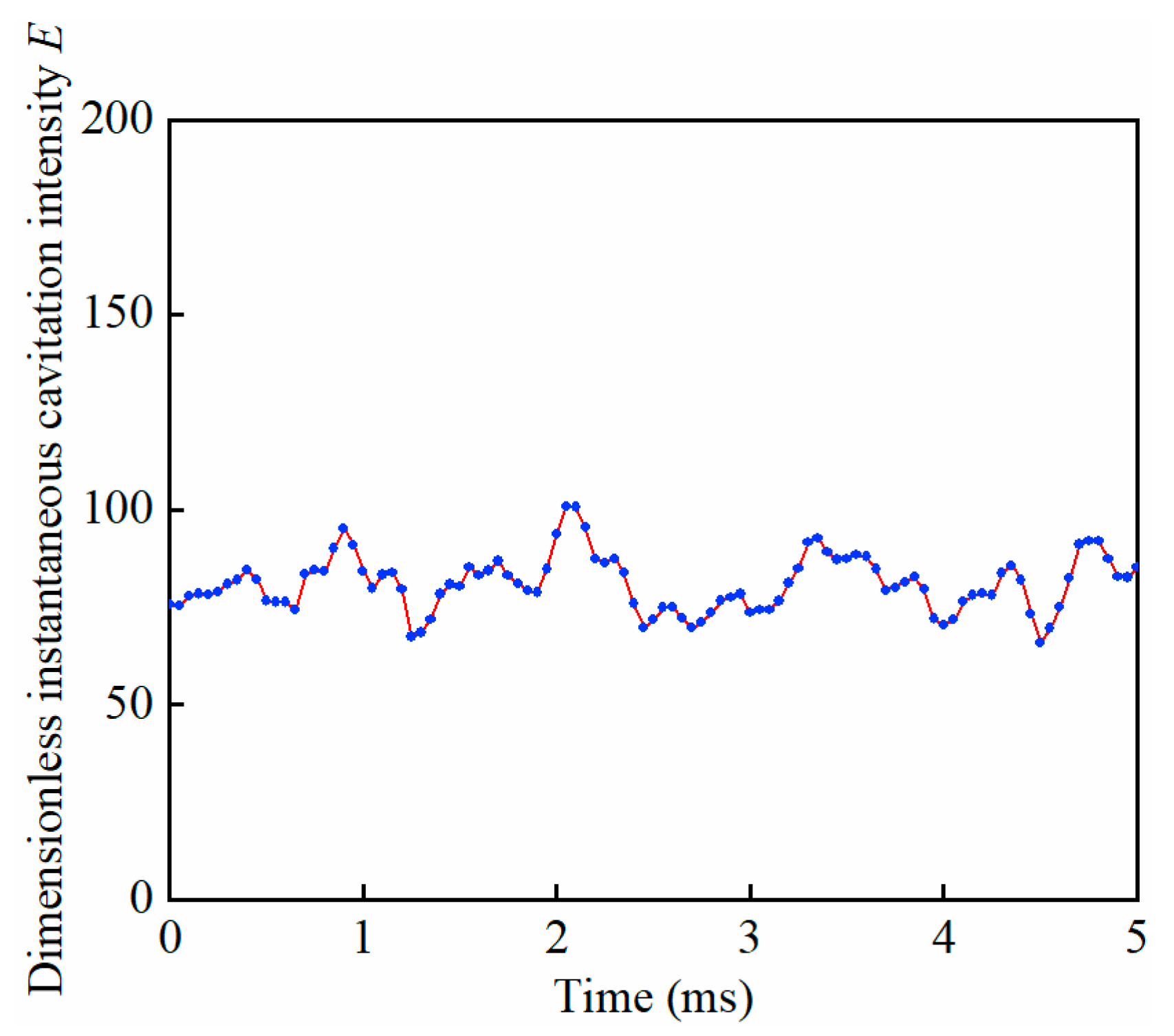
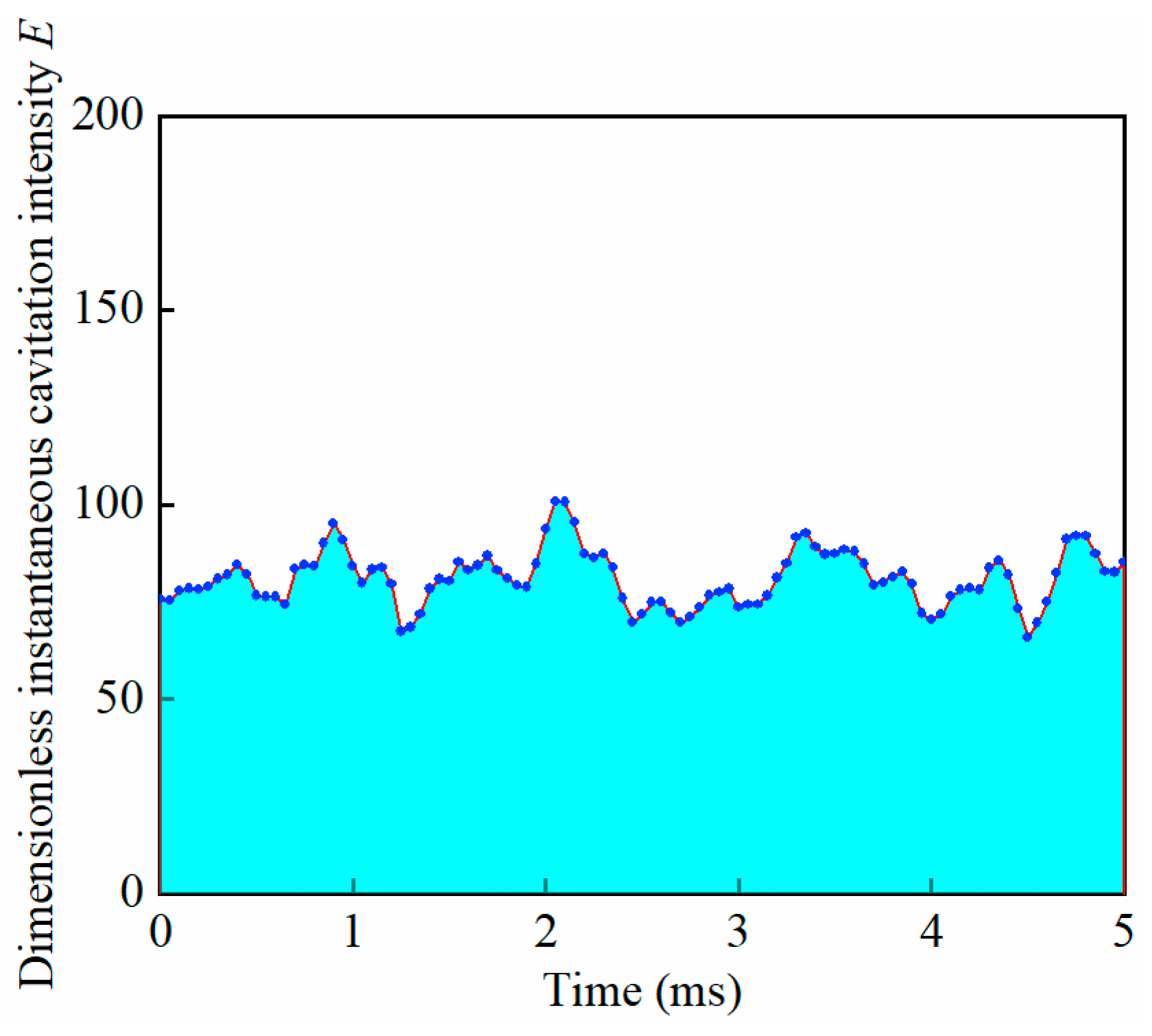
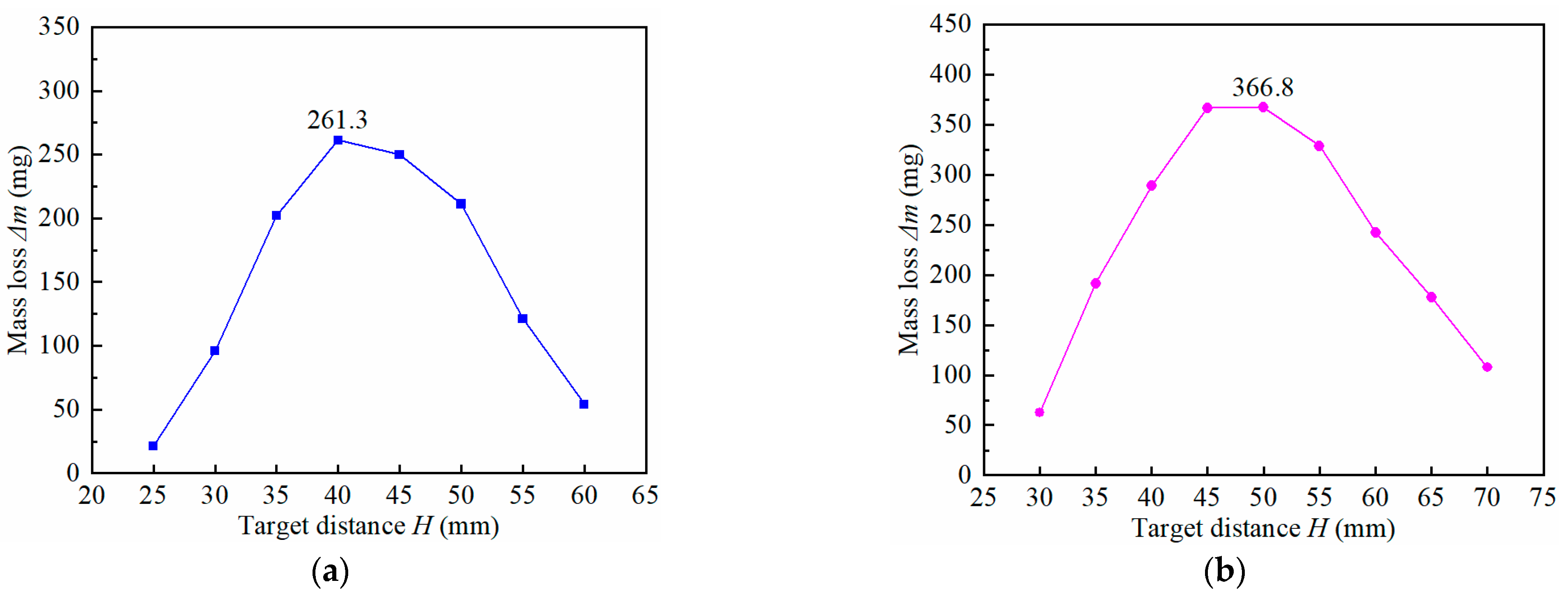
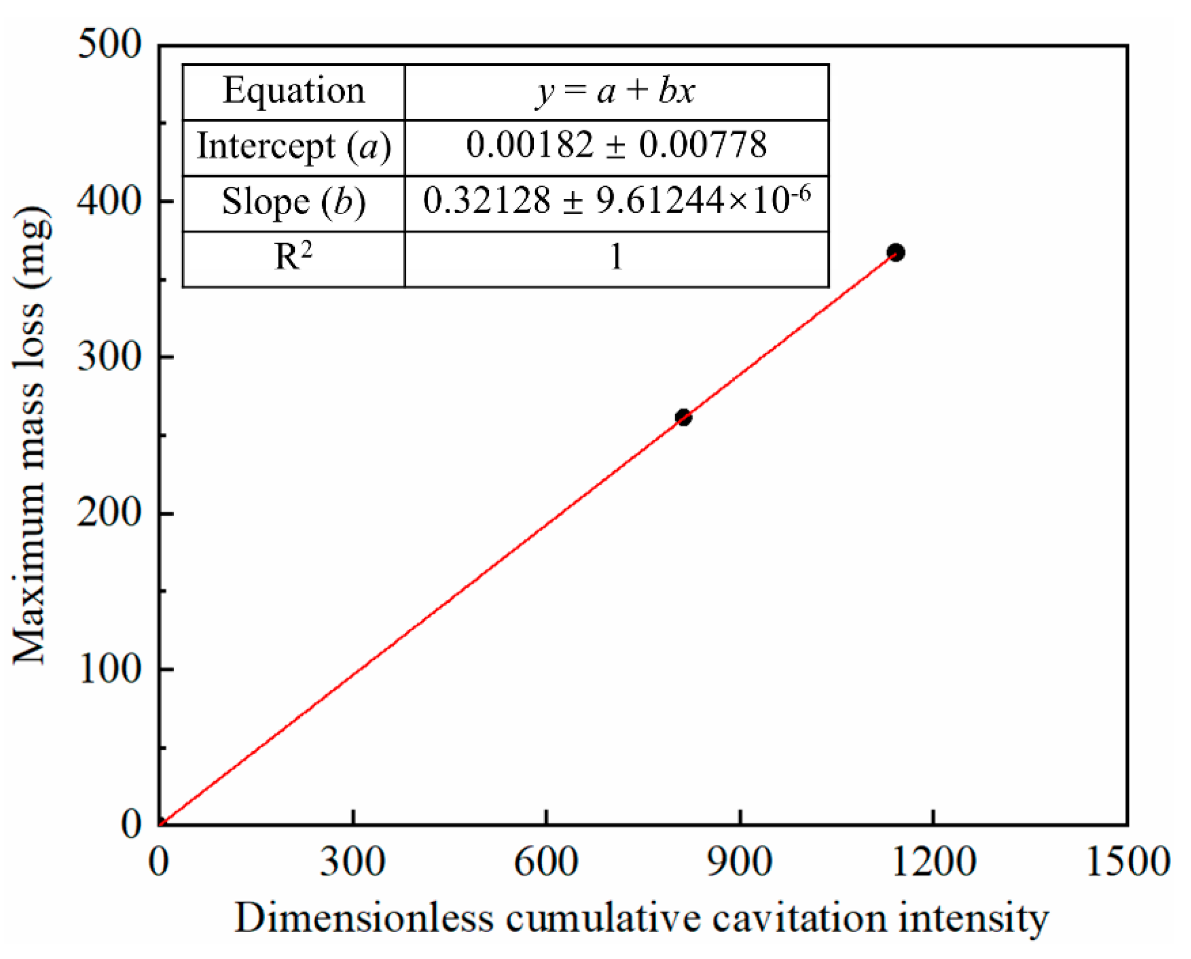
2.3. Erosion Intensity Evaluation

Since mass loss is an intuitive indicator of the degree of erosion of a sample, this factor was used to directly reflect the erosion capacity of the submerged cavitation jet. The more mass loss, the higher erosion capacity. On the contrary, less mass loss indicates that the erosion capacity is weaker. Therefore, this paper takes the mass loss of the sample after erosion as an indicator for evaluating the erosion capacity of the submerged cavitation jet. A 1060 aluminum sheet (not heat treated) was used to create the samples for the erosion experiment; its chemical composition and physical properties are shown in Table 2 and Table 3, respectively. The mass of the sample was accurately weighed using an electronic analytical balance with an accuracy of 0.1 mg. The difference in mass of the sample before and after the erosion experiment was defined as the mass loss of the sample, Δm.
Before each experiment, the samples were ultrasonically cleaned in absolute ethanol for 5 min and then dried. An electronic analytical balance was used to weigh the samples three times. The average value was taken as the mass of the samples before the experiment. Then, the samples were fixed to a clamp and the clamp was fixed to the bottom of the working water tank. The pressure-regulating valve was adjusted to a preset working pressure and the experimental nozzle to a preset target distance. The relief valve and the control valve were turned on to keep the pipeline smooth. Each experiment was conducted for 30 min. After the experiment, the samples were carefully removed and dried. The samples were once again ultrasonically cleaned in pure ethanol for 5 min and then dried. The electronic analytical balance was used to weigh the samples three times. The average value was taken as the mass of the sample after the experiment. The mass loss of the sample for each experiment was then calculated. Finally, the maximum mass loss of the sample was obtained and used to directly evaluate the maximum erosion capacity of the submerged cavitation jet.

3. Results and Discussion

As shown in Figure 6, the dynamic changes of the cavitation clouds were periodic. They can be divided into four stages: inception, growth, shedding, and collapse. This indicates that the cavitation intensity of the submerged cavitation jet is periodic, which means that the cavitation intensity in the cavitation cloud itself also changes periodically with the state of the cavitation cloud. After processing the cavitation cloud images using the dimensionless grayscale intensity method, it can be seen that the distribution of intensity of the cavitation cloud differs over time and space, as shown in Figure 7. In the figure, a dimensionless grayscale intensity value of 1 indicates the highest density of cavitation bubbles in the region, and a value of 0 indicates that there are no cavitation bubbles in the region. The collapse of a cavitation cloud decreases the density of cavitation bubbles, while the inception and growth of a cavitation cloud in the next stage increases the density of cavitation bubbles. As the cavitation cloud changes over time, the density of cavitation bubbles also changes. This also shows that the cavitation intensity produced by the submerged cavitation jet is fluctuating and periodic.
The dimensionless cavitation intensity of a single cavitation cloud image can be obtained from the surface integral of the dimensionless grayscale intensity. The dimensionless cavitation intensity of a single cavitation cloud image is expressed as the dimensionless cavitation intensity produced by the submerged cavitation jet at a certain transient moment. Figure 8 shows the dimensionless instantaneous cavitation intensity produced by the submerged cavitation jet when the working pressure is 10 MPa and 15 MPa. These results were obtained by processing 200 continuous cavitation cloud images over 10 ms. It can be further confirmed from the figure that the dimensionless instantaneous cavitation intensity produced by the submerged cavitation jet was fluctuating and periodic. On this basis, the dimensionless cumulative cavitation intensity produced by the submerged cavitation jet under various working conditions can be obtained using the time integral of the dimensionless instantaneous cavitation intensity. Based on the time integral, the dimensionless cumulative cavitation intensity was found to be 813.277 and 1141.682 at working pressures of 10 MPa and 15 MPa, respectively.
Figure 9 shows how the mass loss of the sample changed with target distance while undergoing erosion by a submerged cavitation jet at two different working pressures. Initially, as the target distance increased, the cavitation cloud developed strongly, and the erosion caused by the collapse of the cavitation bubbles as they reached the target’s surface increased, resulting in an increase in the mass loss of the sample. Next, as the target distance increases, the cavitation cloud began to shed and collapse, the number of cavitation bubbles reaching the target surface decreased, and the erosion weakened, resulting in a decrease in mass loss of the sample after reaching a peak value. As can also be seen from Figure 9, at working pressures of 10 MPa and 15 MPa, mass loss peaked at the target distances of 40 mm and 50 mm and peak values of 261.3 mg and 366.8 mg, respectively. As described above, the erosion capacity of a submerged cavitation jet can be directly evaluated via the mass loss of the sample. The greater the mass loss, the higher the jet’s erosion capacity. Therefore, it can be stated that the erosion capacity of the submerged cavitation jet was strongest at the target distance of 40 mm when working at 10 MPa and a distance of 50 mm at 15 MPa. In order to establish the relationship between the erosion capacity of the submerged cavitation jet and the cavitation cloud images, the maximum mass loss of the sample and the dimensionless cumulative cavitation intensity of the cavitation cloud images were curve-fitted, as shown in Figure 10. It can be easily seen that there is an excellent linear relationship between these factors. The erosion capacity of the submerged cavitation jet can be obtained directly by using the image processing method based on dimensionless grayscale intensity. Therefore, the erosion capacity of the submerged cavitation jets can be quantitatively evaluated by the image processing method proposed in this paper.
In order to verify the accuracy of the dimensionless grayscale intensity image processing method proposed in this paper, the same erosion experiment was carried out at a working pressure of 20 MPa. The image of the cavitation cloud was captured by the high-speed camera. Two hundred continuous cavitation cloud images were selected covering 10 ms. According to the image processing method, the dimensionless cumulative cavitation intensity produced by the submerged cavitation jet at the working pressure of 20 MPa was 1255.033. Based on the fitting curve in Figure 10, it can be calculated that the peak mass loss of the sample was 403.2 mg when the working pressure was 20 MPa. On the other hand, according to the results shown in Figure 11, when the working pressure was 20 MPa and the target distance was 55 mm, the mass loss of the reached a peak of 398.2 mg. Comparing the image processing result with the experimental result, the error between them is 1.26%, as shown in Table 4. This proves that the image processing method based on the dimensionless grayscale intensity proposed in this paper can be used to evaluate the performance of the submerged cavitation jet quantitatively and accurately. As a result, this image processing method can significantly reduce the time and cost of testing the performance of cavitation nozzles.
The error caused by image noise may be accumulated and amplified during the process of integration, leading to an increase in the calculation error of the maximum mass loss, which affects the evaluation of the submerged cavitation jet’s performance. For this purpose, variation in the calculation error of the maximum mass loss for the sample space from 10 to 5000 images when the working pressure is 20 MPa was investigated, as shown in Figure 12. It can be seen from the figure that the calculation errors of the maximum mass loss in different image sample spaces were all below 3.29%. This result further proves the accuracy and reliability of the image processing method proposed in this paper for quantitatively evaluating the submerged cavitation jet performance.

4. Conclusions

In order to obtain a quantitative evaluation of the performance of submerged cavitation jets, a novel image processing method based on dimensionless grayscale intensity was proposed. According to the results, the following conclusions can be drawn:
(1)
The image processing method based on the dimensionless grayscale intensity can quantitatively and accurately evaluate the performance of the submerged cavitation jet.
(2)
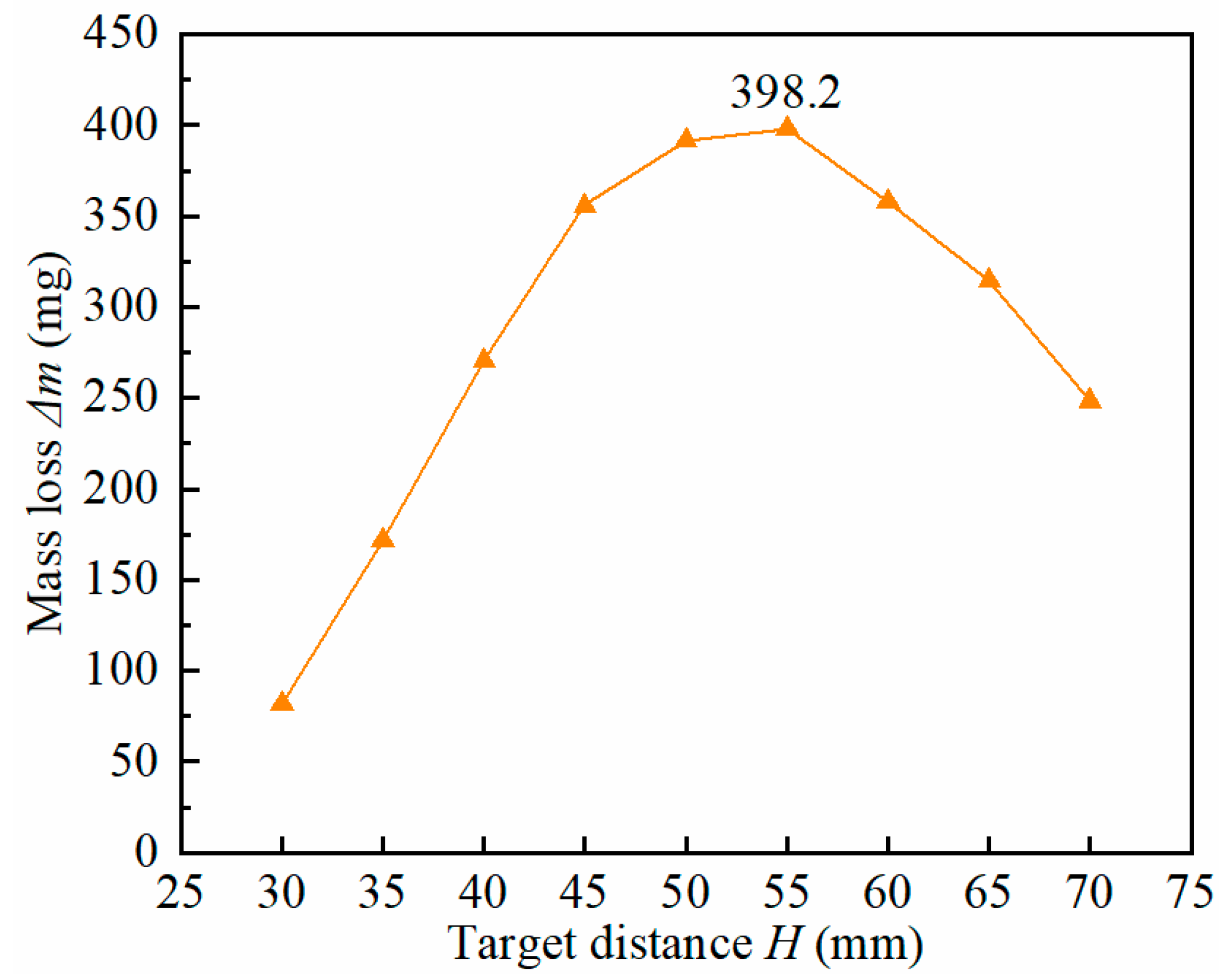
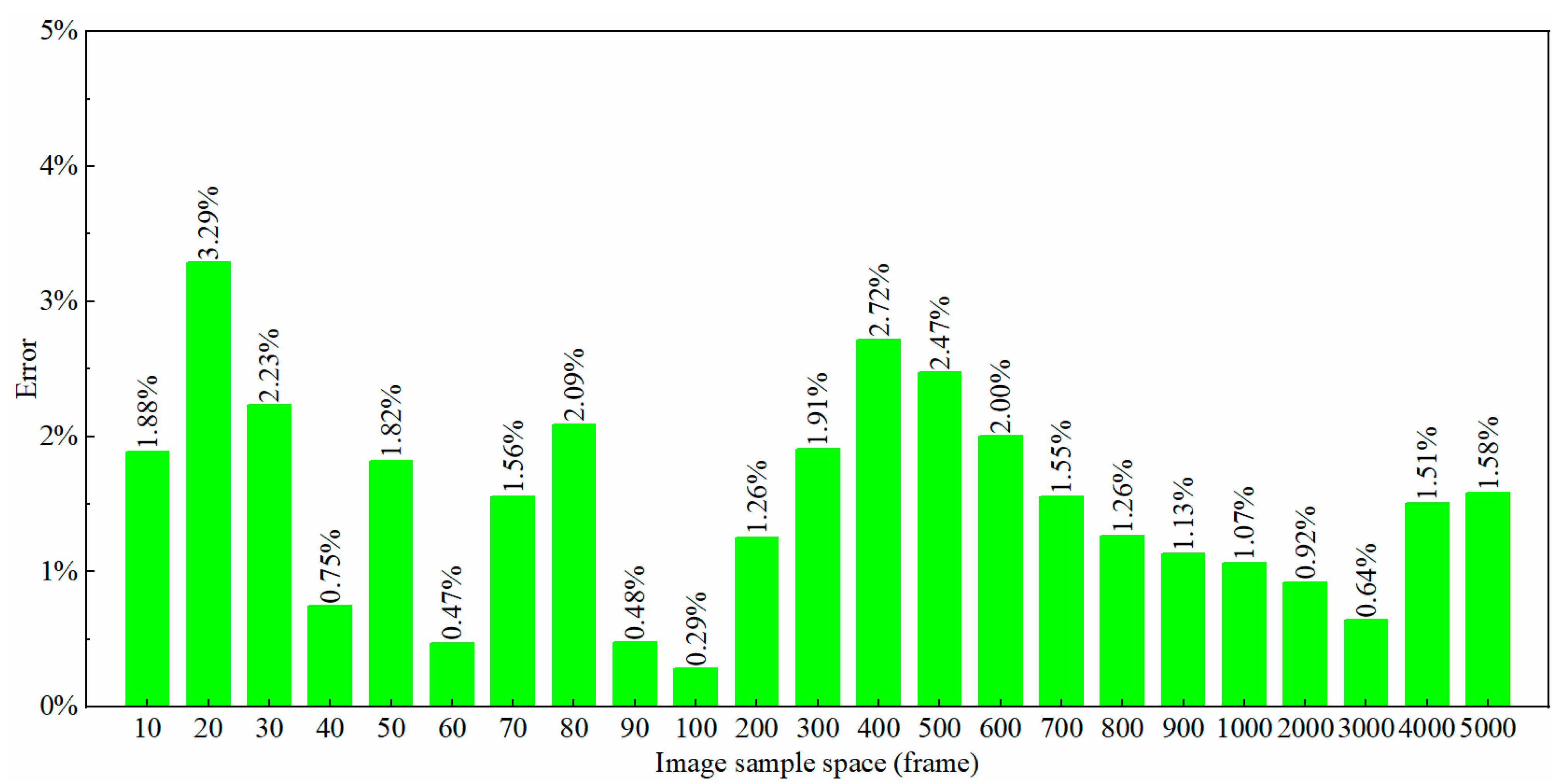
When the sample space is 200 images and the working pressure was 20 MPa, the calculation error of the image processing method for the maximum mass loss of the sample was 1.26%.
(3)
For the sample space of 10–5000 images, the calculation errors of the image processing method for the maximum mass loss of samples were all within 3.29%.

Author Contributions

Conceptualization, investigation, writing and editing, project administration, funding acquisition, J.D.; validation, investigation, writing and editing, X.Z.; methodology, R.M.; investigation, M.L.; project administration, funding acquisition, X.P. All authors have read and agreed to the published version of the manuscript.

Funding

This research was funded by National Natural Science Foundation of China, grant number 51979022, and Fundamental Research Funds for the Central Universities grant number 3132019330.

Institutional Review Board Statement

Not applicable.

Informed Consent Statement

Not applicable.

Conflicts of Interest

The authors declare no conflict of interest.

References

  1. Song, C.; Cui, W. Review of Underwater Ship Hull Cleaning Technologies. J. Mar. Sci. Appl. 2020, 19, 415–429. [Google Scholar] [CrossRef]
  2. Perrin, L.; Colombet, D.; Ayela, F. Comparative study of luminescence and chemiluminescence in hydrodynamic cavitating flows and quantitative determination of hydroxyl radicals production. Ultrason. Sonochem. 2020, 70, 105277. [Google Scholar] [CrossRef] [PubMed]
  3. Podbevšek, D.; Colombet, D.; Ayela, F.; Ledoux, G. Localization and quantification of radical production in cavitating flows with luminol chemiluminescent reactions. Ultrason. Sonochem. 2020, 71, 105370. [Google Scholar] [CrossRef] [PubMed]
  4. Zhao, F.; Wang, X.; Xu, W.; Zhao, Y.; Zhao, G.; Zhu, H. Study on Different Parameters of the Self-Excited Oscillation Nozzle for Cavitation Effect under Multiphase Mixed Transport Conditions. J. Mar. Sci. Eng. 2021, 9, 1159. [Google Scholar] [CrossRef]
  5. El Hassan, M.; Bukharin, N.; Al-Kouz, W.; Zhang, J.-W.; Li, W.-F. A Review on the Erosion Mechanism in Cavitating Jets and Their Industrial Applications. Appl. Sci. 2021, 11, 3166. [Google Scholar] [CrossRef]
  6. Bukharin, N.; El Hassan, M.; Omelyanyuk, M.; Nobes, D. Applications of cavitating jets to radioactive scale cleaning in pipes. Energy Rep. 2020, 6, 1237–1243. [Google Scholar] [CrossRef]
  7. Chong, Z.R.; Yang, S.H.B.; Babu, P.; Linga, P.; Li, X.-S. Review of natural gas hydrates as an energy resource: Prospects and challenges. Appl. Energy 2016, 162, 1633–1652. [Google Scholar] [CrossRef]
  8. Zhang, Y.; Zhao, K.; Wu, X.; Tian, S.; Shi, H.; Wang, W.; Zhang, P. An innovative experimental apparatus for the analysis of natural gas hydrate erosion process using cavitating jet. Rev. Sci. Instrum. 2020, 91, 095107. [Google Scholar] [CrossRef]
  9. Hutli, E.; Nedeljkovic, M.S.; Bonyár, A.; Légrády, D. Experimental study on the influence of geometrical parameters on the cavitation erosion characteristics of high speed submerged jets. Exp. Therm. Fluid Sci. 2017, 80, 281–292. [Google Scholar] [CrossRef]
  10. Peng, C.; Tian, S.; Li, G.; Wei, M. Enhancement of cavitation intensity and erosion ability of submerged cavitation jet by adding micro-particles. Ocean Eng. 2020, 209, 107516. [Google Scholar] [CrossRef]
  11. Li, D.; Kang, Y.; Ding, X.; Liu, W. Experimental study on the effects of feeding pipe diameter on the cavitation erosion performance of self-resonating cavitating waterjet. Exp. Therm. Fluid Sci. 2017, 82, 314–325. [Google Scholar] [CrossRef]
  12. Cai, T.; Pan, Y.; Ma, F. Effects of nozzle lip geometry on the cavitation erosion characteristics of self-excited cavitating waterjet. Exp. Therm. Fluid Sci. 2020, 117, 110137. [Google Scholar] [CrossRef]
  13. Hutli, E.; Petrović, P.B.; Nedeljkovic, M.; Legrady, D. Automatic Edge Detection Applied to Cavitating Flow Analysis: Cavitation Cloud Dynamics and Properties Measured through Detected Image Regions. Flow Turbul. Combust. 2021, 108, 865–893. [Google Scholar] [CrossRef]
  14. Soyama, H. Cavitating Jet: A Review. Appl. Sci. 2020, 10, 7280. [Google Scholar] [CrossRef]
  15. Zhang, F.; Liu, H.; Xu, J.; Tang, C. Experimental investigation on noise of cavitation nozzle and its chaotic behaviour. Chin. J. Mech. Eng. 2013, 26, 758–762. [Google Scholar] [CrossRef]
  16. Liao, H.-L.; Zhao, S.-L.; Cao, Y.-F.; Zhang, L.; Yi, C.; Niu, J.-L.; Zhu, L.-H. Erosion characteristics and mechanism of the self-resonating cavitating jet impacting aluminum specimens under the confining pressure conditions. J. Hydrodyn. 2020, 32, 375–384. [Google Scholar] [CrossRef]
  17. Wang, X.; Li, Y.; Hu, Y.; Ding, X.; Xiang, M.; Li, D. An Experimental Study on the Jet Pressure Performance of Organ–Helmholtz (O-H), Self-Excited Oscillating Nozzles. Energies 2020, 13, 367. [Google Scholar] [CrossRef]
  18. Liu, C.; Liu, G.; Yan, Z. Study on Cleaning Effect of Different Water Flows on the Pulsed Cavitating Jet Nozzle. Shock Vib. 2019, 2019, 1–15. [Google Scholar] [CrossRef]
  19. Shafaghi, A.H.; Talabazar, F.R.; Zuvin, M.; Gevari, M.T.; Villanueva, L.G.; Ghorbani, M.; Koşar, A. On cavitation inception and cavitating flow patterns in a multi-orifice microfluidic device with a functional surface. Phys. Fluids 2021, 33, 032005. [Google Scholar] [CrossRef]
  20. Talabazar, F.R.; Jafarpour, M.; Zuvin, M.; Chen, H.; Gevari, M.T.; Villanueva, L.G.; Grishenkov, D.; Koşar, A.; Ghorbani, M. Design and fabrication of a vigorous “cavitation-on-a-chip” device with a multiple microchannel configuration. Microsystems Nanoeng. 2021, 7, 1–13. [Google Scholar] [CrossRef]
  21. Hutli, E.A.F.; Nedeljkovic, M. Frequency in Shedding/Discharging Cavitation Clouds Determined by Visualization of a Submerged Cavitating Jet. J. Fluids Eng. 2008, 130, 021304. [Google Scholar] [CrossRef]
  22. Wright, M.M.; Epps, B.; Dropkin, A.; Truscott, T.T. Cavitation of a submerged jet. Exp. Fluids 2013, 54, 1541. [Google Scholar] [CrossRef]
  23. Sato, K.; Taguchi, Y.; Hayashi, S. High Speed Observation of Periodic Cavity Behavior in a Convergent-Divergent Nozzle for Cavitating Water Jet. J. Flow Control. Meas. Vis. 2013, 01, 102–107. [Google Scholar] [CrossRef]
  24. Hutli, E.; Nedeljkovic, M.; Bonyár, A. Dynamic behaviour of cavitation clouds: Visualization and statistical analysis. J. Braz. Soc. Mech. Sci. Eng. 2019, 41, 281. [Google Scholar] [CrossRef]
  25. Wu, Q.; Wei, W.; Deng, B.; Jiang, P.; Li, D.; Zhang, M.; Fang, Z. Dynamic characteristics of the cavitation clouds of submerged Helmholtz self-sustained oscillation jets from high-speed photography. J. Mech. Sci. Technol. 2019, 33, 621–630. [Google Scholar] [CrossRef]
  26. Hayashi, S.; Sato, K. Unsteady Behavior of Cavitating Waterjet in an Axisymmetric Convergent-Divergent Nozzle: High Speed Observation and Image Analysis Based on Frame Difference Method. J. Flow Control. Meas. Vis. 2014, 02, 94–104. [Google Scholar] [CrossRef]
  27. Yang, Y.; Li, W.; Shi, W.; Wang, C.; Zhang, W. Experimental Study on Submerged High-Pressure Jet and Parameter Optimization for Cavitation Peening. Mechanika 2020, 26, 346–353. [Google Scholar] [CrossRef]
  28. Sekyi-Ansah, J.; Wang, Y.; Tan, Z.; Zhu, J.; Li, F. The Dynamic Evolution of Cavitation Vacuolar Cloud with High-Speed Camera. Arab. J. Sci. Eng. 2020, 45, 4907–4919. [Google Scholar] [CrossRef]
  29. Dong, J.; Li, S.; Meng, R.; Zhong, X.; Pan, X. Research on Cavitation Characteristics of Two-Throat Nozzle Submerged Jet. Appl. Sci. 2022, 12, 536. [Google Scholar] [CrossRef]
  30. Fujisawa, N.; Fujita, Y.; Yanagisawa, K.; Fujisawa, K.; Yamagata, T. Simultaneous observation of cavitation collapse and shock wave formation in cavitating jet. Exp. Therm. Fluid Sci. 2018, 94, 159–167. [Google Scholar] [CrossRef]
  31. Watanabe, R.; Yanagisawa, K.; Yamagata, T.; Fujisawa, N. Simultaneous shadowgraph imaging and acceleration pulse measurement of cavitating jet. Wear 2016, 358–359, 72–79. [Google Scholar] [CrossRef]
  32. Peng, C.; Tian, S.; Li, G. Joint experiments of cavitation jet: High-speed visualization and erosion test. Ocean Eng. 2018, 149, 1–13. [Google Scholar] [CrossRef]
  33. Peng, C.; Tian, S.-C.; Li, G.-S. Determination of the shedding frequency of cavitation cloud in a submerged cavitation jet based on high-speed photography images. J. Hydrodyn. 2021, 33, 127–139. [Google Scholar] [CrossRef]
  34. Zhong, X.; Dong, J.; Liu, M.; Meng, R.; Li, S.; Pan, X. Experimental study on ship fouling cleaning by ultrasonic-enhanced submerged cavitation jet: A preliminary study. Ocean Eng. 2022, 258. [Google Scholar] [CrossRef]
  35. Yang, Y.; Li, W.; Shi, W.; Zhou, L.; Zhang, W. Experimental Study on the Unsteady Characteristics and the Impact Performance of a High-Pressure Submerged Cavitation Jet. Shock Vib. 2020, 2020, 1–15. [Google Scholar] [CrossRef]
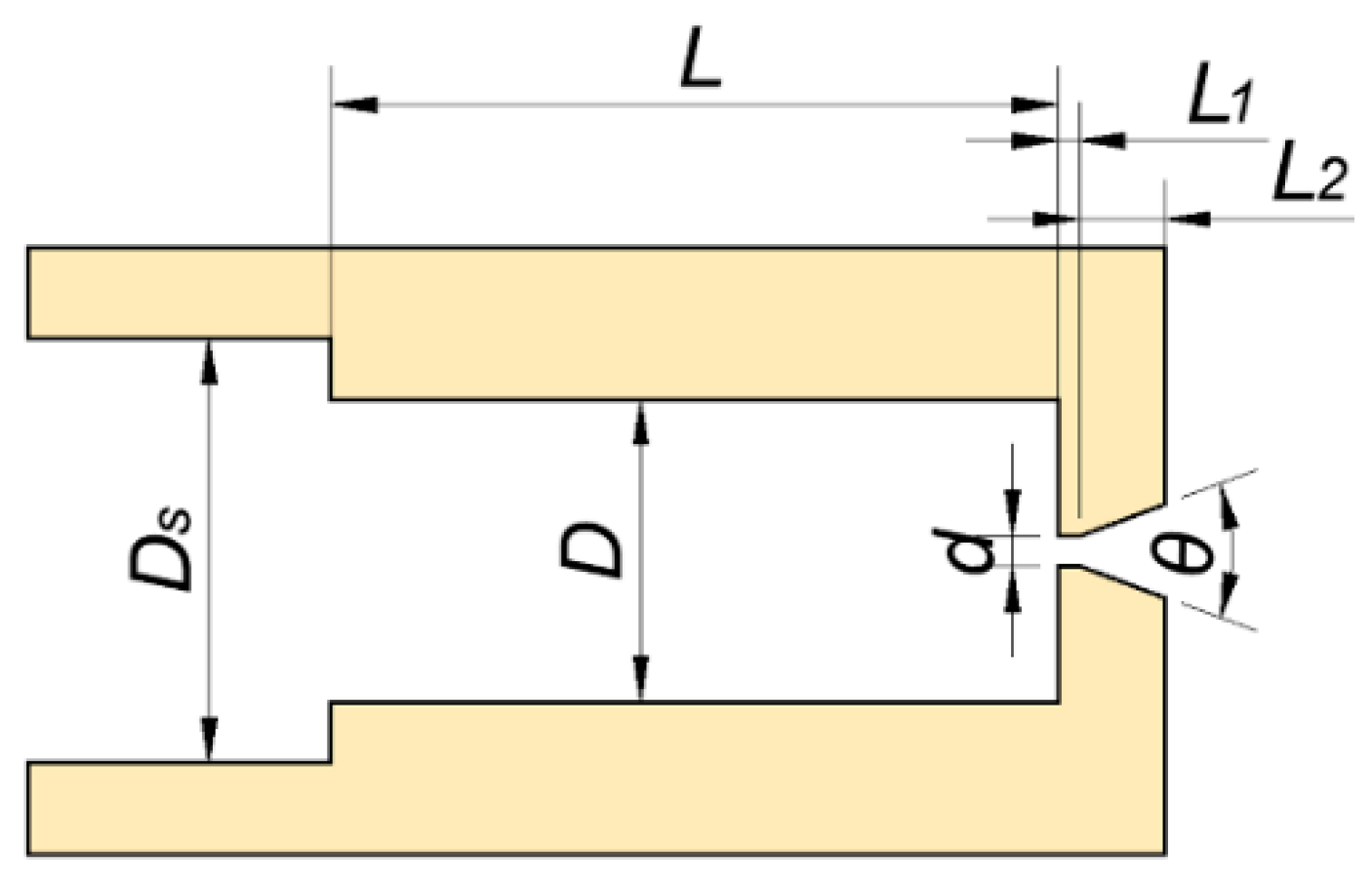
Figure 1. Schematic diagram of experimental setup for the submerged cavitation jet.
Jmse 10 01336 g001
Figure 2. Schematic diagram of the experimental nozzle.
Jmse 10 01336 g002
Figure 3. The dimensionless grayscale intensity distribution of the cavitation cloud image after image processing.
Jmse 10 01336 g003
Figure 4. Variation in dimensionless instantaneous cavitation intensity over time, obtained by means of image processing.
Jmse 10 01336 g004
Figure 5. Dimensionless cumulative cavitation intensity after the time integral.
Jmse 10 01336 g005
Figure 6. Variation of cavitation cloud with time at a working pressure of 10 MPa.
Jmse 10 01336 g006
Figure 7. Space–time distribution of dimensionless grayscale intensity of cavitation cloud at a working pressure of 10 MPa.
Jmse 10 01336 g007
Figure 8. Dimensionless instantaneous cavitation intensity obtained by image processing: (a) at a working pressure of 10 MPa; (b) at a working pressure of 15 MPa.
Jmse 10 01336 g008
Figure 9. Mass loss of the sample: (a) at a working pressure of 10 MPa; (b) at a working pressure of 15 MPa.
Jmse 10 01336 g009
Figure 10. Fitting curve of dimensionless cumulative cavitation intensity and maximum mass loss.
Jmse 10 01336 g010
Figure 11. Mass loss of the sample at a working pressure of 20 MPa.
Jmse 10 01336 g011
Figure 12. Calculation errors of maximum mass loss of the sample.
Jmse 10 01336 g012
Table 1. The dimensions of the experimental nozzle.
Parameter DescriptionSymbolValueUnits
Diameter of nozzle inletDs14mm
Diameter of resonant cavityD10mm
Diameter of minimum throat diameterd1mm
Length of resonant cavityL24mm
Length of minimum throatL10.7mm
Length of nozzle exit lipL22.8mm
Nozzle exit expansion angleθ40°
Table 2. Chemical composition of the samples (mass fraction).
AlFeSiCuZnVMnMgTi
99.6≤0.35≤0.25≤0.05≤0.05≤0.05≤0.03≤0.03≤0.03
Table 3. Physical properties of the samples.
Density
/kg∙m3
Tensile Strength /MPaElasticity Modulus /GPaOffset Yield Strength
/MPa
Vickers Hardness HV0.2Surface Roughness
/μm
2710807135311
Table 4. Comparison of the image processing result with the experimental result.
Working Pressure
/MPa
Image Processing Result
/mg
Experimental Result
/mg
Error
20403.2398.21.26%
Publisher’s Note: MDPI stays neutral with regard to jurisdictional claims in published maps and institutional affiliations.

