1. Introduction
Establishing connections between trees, manifolds, pipe terminationsand risers, the subsea jumper is essential to the oil and gas production system. Unlike other subsea pipelines, jumpers have unique structural forms, such as multiple bends and long suspension spans. These forms are more likely to vibrate under the motion of internal multiphase flow, resulting in pipeline instability, strength failure, or fatigue failure [
1].
As a jumper consists of several straight pipes and elbows, some conclusions and methods for investigating the flow and vibration patterns of those structures are still applicable to the jumper. The effect of flow parameters and pipe geometry on the two-phase flow patterns in horizontal straight pipes, especially the slug flow, has been widely analyzed by experimental and numerical methods in Carvalho, et al. [
2], Bamidele, et al. [
3], Orres, et al. [
4], Xu et al. [
5], Baumann, et al. [
6], and Dinayanto, et al. [
7]. The related stress analysis for gas–liquid flow inside a straight pipe and the application of fluid–structure coupling to model the vibration response have also been mentioned in previous studies by Mohmmed, et al. [
8] and Al-Hashimy, et al. [
9]. Miwa, et al. [
10] and Bamidele, et al. [
11] experimentally investigated the two-phase flow-induced wave dynamics in a 90° elbow to obtain the forces and associated flow parameters such as the volume flow rate, void ratio fluctuations, and local pressure distribution around the elbow. Oscillatory flow-induced force fluctuations due to specific stratified wave flow analysis are derived from momentum, pressure, and collision effect fluctuations. The internal flow characteristics inside U-bends, blind tees, and T-joints under different flow conditions have also been studied experimentally and numerically by Han et al. [
12], Santos and Kawaji [
13], Han, et al. [
14], and Chen, et al. [
15], etc. The flow of gas–liquid in the pipes, according to the flow direction and void fraction, can be determined by the different flow regimes shown in
Figure 1.
Existing studies on the vibration of subsea pipelines mainly focus on in-line planar pipelines and the corresponding vortex-induced vibrations caused by the oscillatory lift force generated by the vortex shedding [
17,
18,
19,
20,
21,
22]. With the development of deepwater oil and gas exploitation technology, the pressure and flow rate in the pipeline gradually increase. Therefore, the internal flow-induced vibration (FIV) problem of subsea jumpers has been receiving increasing attention in the offshore engineering community. Holmes and Constantinides [
23] and Zhu, et al. [
24] conducted experimental and computational fluid dynamics (CFD) studies to predict internal-flow-induced vibration of subsea pipelines. With regard to the vibration in the subsea jumper, most studies on jumpers have focused on M-shaped and U-shaped jumpers by using numerical methods [
25]. Talley, et al. [
26] found that compared to single-phase flow, the vibration amplitude caused by two-phase flow is more significantly influenced by the flow properties of density, flow velocity, and void fraction. On this basis, Chica, et al. [
27] conducted a numerical study using CFD coupled with a finite element method to analyze the vibrations induced by plug flow in the middle section of a rigid M-shaped jumper and evaluate its effect on fatigue life. Elyyan, et al. [
28] carried out a numerical study of subsea M-shaped jumper, using one-way FSI (fluid–structure interaction) methods to capture fluid–structure interactions and evaluate hydrodynamically induced pipe deformations. This study proved that the one-way FSI is enough to catch the main deformation and major frequencies under controlled operating conditions. Chen et al. [
29] studied the failure pressure of high-strength pipes by using the nonlinear finite element analysis method. However, to the authors’ knowledge, the experimental work for multiphase flow-induced vibration is still missing.
Due to the limitations of in-line planar jumpers such as M-shaped, U-shaped, and reverse U-shaped jumpers, the industry is turning to multi-plane jumper systems such as Z-shaped and three-dimensional irregular jumpers. These jumpers increase tolerance for end displacement and are designed to be customized to accommodate the periodic end movements of subsea structures. Studies on multi-planar jumpers were rare, and only a few numerical analyses on internal flow characteristics such as slug flow were carried out by Wang, et al. [
30], Dai, et al. [
31], Lu, et al. [
32], and Song, et al. [
33]. Nair, et al. [
34] analyzed the vibration fatigue response of a multi-plane jumper structure for an internal slug. Numerical simulations of the internal flow in the jumper were carried out to obtain the pressure fluctuations on the jumper, which were used to determine the fatigue damage to the slug. Pontaza and Menon [
35] conducted three-dimensional numerical simulations of the vibration process caused by unsteady multiphase flow in a transverse tube to estimate the structural response of the jumper. However, most methods in existing studies are mainly based on numerical simulations, which are incapable of capturing real fluid–structure interactions and also introduce significant uncertainties and may produce conservative solutions in most applications. Previous studies of applying FSI techniques on rigid pipes are rare, and experimental tests are limited. A detailed comparison of experimental measurement and numerical results of the two-phase internal flow interaction with rigid jumpers is required to evaluate the prediction performance for the vibration response induced by the two-phase pipe flow of the numerical simulations.
In the present study, the characteristics of the gas–liquid flow and the induced vibration in a multi-plane Z-shaped jumper are investigated by adopting experimental and numerical techniques. Flow visualization in seven different sections is carried out using a high-speed camera in the experiment. Both displacement and pressure sensors are used to record the vibration and pressure responses of the jumper, which is analyzed with different gas content rates, mixing velocities, and gas and liquid surface velocities. Numerical simulations based on the VOF method and one-way fluid–solid coupling are performed to analyze the interactions between the multiphase flow and the jumper with different gas–liquid velocities. The paper is organized as follows. Part 2 briefly describes the multiphase flow experimental setup of the present study. Part 3 presents the numerical model of the fluid–solid coupling and the mesh convergence analysis. In Part 4, experimental studies on the evolution of the flow pattern, vibration characteristics, and pressure distribution under specific cases are conducted, and the effects of two-phase flow parameters on the flow and vibration characteristics are analyzed. In Part 5, the results of the numerical simulations are conducted, and the results are compared with the experimental measurements. Finally, conclusions are presented in Part 6.
2. Experimental Set-Up
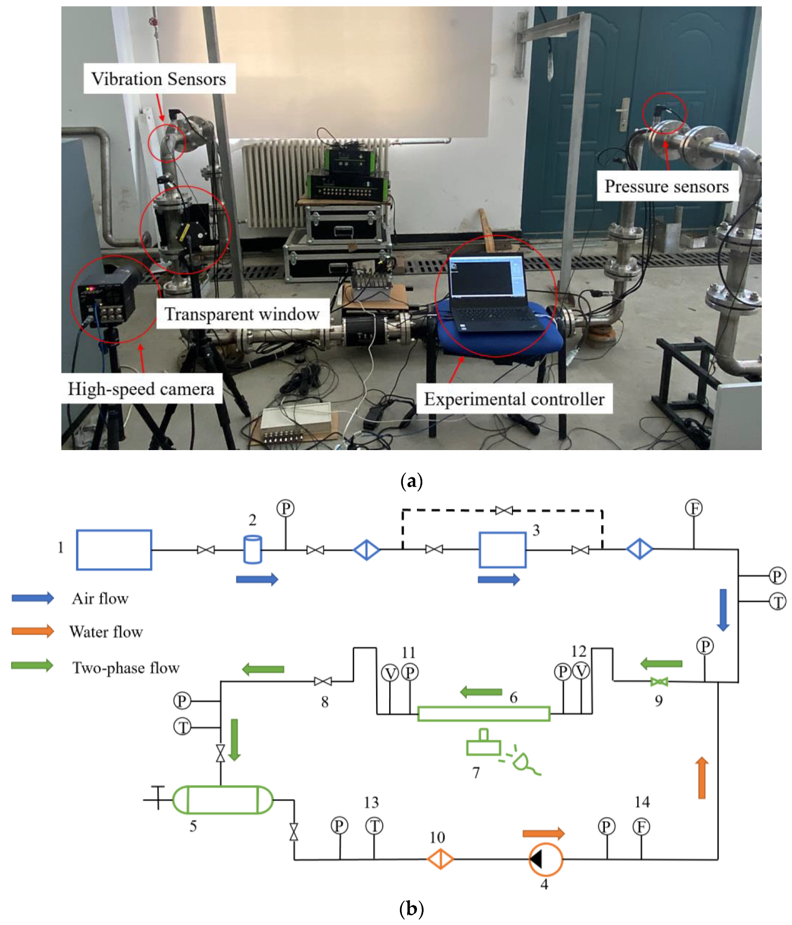
A multiphase flow experimental set-up as shown in
Figure 2 is established to study the flow characteristics and flow-induced vibration of multi-plane jumper gas–liquid two-phase flow.
In the experiment, compressed air is used as the gas-phase medium by two air compressors (1 in
Figure 2b) with a maximum exhaust pressure of 20 bar. After coming out of the air bottle (2 in
Figure 2b), the compressed air is dried by the freeze dryer (3 in
Figure 2b). Before joining the gas–liquid mixed section, a gas mass flow meter is used to measure the gas flow rate. Water is selected as the liquid phase and sent into the test section through a centrifugal water pump (4 in
Figure 2b) whose motor is designed based on frequency conversion, with a frequency range between 10 and 50 Hz. The flow rate of the single pump is up to 100 m³/h. The flow valve and pump frequency conversion are controlled by the Proportional-integral-derivative (PID) methodology. After the air and water are fully mixed in the gas–liquid mixing section, the two-phase flow enters the experimental pipeline by opening and closing the specific ball valves (9 in
Figure 2b). After the flow passes the jumper, it enters the three-phase separator (5 in
Figure 2b) through the return pipeline, with air going to the top and water entering the bottom. A centrifugal pump finally sends the separated fluids to the loop system.
As shown in
Figure 3, the test section is a Z-shaped jumper of inner diameter
D = 48 mm consisting of two ascending sections, two descending sections, three horizontal sections, and six elbows. The jumper sections S1–S7 are designed to be flanged, and each can be replaced by a transparent window of the same size for visualization. The transparent windows are made of Plexiglas with good transparency and can withstand a maximum fluid pressure of 2 MPa. Reinforced supports surrounding the jumper are used to ensure the safety and reliability of the transparent windows and pipeline connections. The jumper is equipped with plug welding support around the bent part of the pipe to install the pressure sensor. The physical parameters of the jumper model are listed in
Table 1, and the properties of the gas–liquid two-phase flow are shown in
Table 2.
A high-speed camera is installed in front of the transparent window to capture the flow characteristics through the jumper. The high-speed camera is a Photron FASTCAM Mini UX100 with a maximum resolution of 1280 × 1024 and a maximum capture speed (full-frame) of 4000 fps. The LED fill light is arranged next to the jumper to ensure sufficient light intensity so that the high-speed camera can capture the water flow.
Eight pressure sensors are installed before and after the elbows of the jumper to monitor the pressure fluctuation of the two-phase flow at different positions. The pressure sensor is a Wika S-20.0-2.5 series, with a range of 0–2.5 MPa and an accuracy is 0.1%, which uses a 0–5 V voltage signal output and is connected to the plug-welded standoffs on the pipeline through NPT threads. The sampling rate is set to 1000 Hz to fully satisfy Nyquist’s law. The data acquisition card uses the NI-USB-6210 series with eight differential signal inputs to ensure accurate and stable data transmission and high response. The NI data acquisition system is installed on the host computer for data acquisition, storage, and export.
Acceleration sensors are installed on the outer wall of the elbow in different sections of the jumper to measure the vibration. The LC0103 internal IC piezoelectric acceleration sensor has good anti-interference and low noise level and is suitable for multi-point measurement, with a sensor sensitivity of 50 mV/g and a frequency range of 0.35–10,000 Hz. The acceleration sensor can be used with the LC3101 data acquisition instrument to achieve multi-channel synchronous sampling. The data can be transferred to the host computer through the USB interface for real-time monitoring in the vibration analysis software for real-time tracking and saving. The time signals of the jumper acceleration response are plotted, and their spectral data are obtained using Fast Fourier Transform (FFT) for analysis.
3. Computational Modeling
3.1. Numerical Method
A computational model of Z-shaped jumper fluid–structure coupling is established based on a VOF multiphase flow model [
36] combined with the k-ωturbulence model [
37]. The one-way fluid–solid coupling based on the pressure-based coupling approach is performed to validate the experimental results, and the finite element method was selected to capture the structural responses.
Without considering the compression of the fluids and the phase change transfer process between the gas and liquid, the governing equations of the fluid domain are the incompressible Navier–Stokes equations including the continuity and momentum equations, which can be written as:
where
ρ and
μ are the density and dynamic viscosity of the fluid,
u = (u, v, w) represents the mean velocity vector of the fluid flow, and
prgh is the dynamic pressure defined as
prgh =
p −
ρg ·
x;
g is the gravitational acceleration vector;
x = (x, y, z) are the Cartesian coordinates;
τ is the specific Reynolds stress tensor written as:
where
μt is the dynamic turbulent eddy viscosity,
is the rate of the strain tensor,
is the anti-symmetric rate of the strain tensor, and
k is the turbulent kinetic energy per unit mass.
The VOF (Volume of Fluid) method is applied to solve for two or more mutually incompatible fluids in the computational domain. The multiphase fluids share the same set of momentum equations in the VOF method, and the volume fraction of each phase in every computational cell is tracked in the entire fluid domain. A variable is introduced for each phase in the model to calculate the volume fraction of each phase in the cell, which is summed to 1 for all phases in each control volume.
where
αq represents the volume fraction of the
q-th phase.
The continuity equation is solved for the volume fraction of each phase to capture the phase interface, and for the
q-th phase, the equation takes the form of:
where
qp is the mass transferred from
q to
p phase;
pq is the mass transferred from
p to
q phase;
ρq is the density of the
q-phase;
Vq is the
q phase velocity;
Sαq is the source term. In the present study, water is regarded as the first phase and air as the second phase. A constant value of 0.072 N/m for the surface tension between the gas and liquid is used. ANSYS FLUENT is used as the solver for the numerical simulations for the above governing equations.
The k-ω turbulence model is used to resolve the turbulence effects, and the standard wall functions are used to resolve the pipe flow boundary layer. The mixing velocity inlet boundary condition is set at the inlet, the pressure outlet boundary condition is established at the outlet, and the no-slip wall boundary condition is used at the wall.
The PISO algorithm is selected to solve the transient simulation; the PRESTO scheme is used for the pressure; the QUICK scheme is used for the momentum equation; the sub-relaxation factors of momentum and pressure are set to 0.3 and 0.7, respectively. The sum of both is 1 to obtain a better convergence speed. The time step is 0.0002 s so that the global Coulomb number is always below 1 to ensure the stability of the simulations.
After obtaining the pressure and vibration by experiment and simulation, the strength calculations can be performed using the equation of p = 2tσ
u/(D-t) [
29], where p is the internal-flow-induced pressure in the pipe; D is the diameter of the pipeline, t is the wall thickness of the pipeline, and σ
u is ultimate tensile strength.
The equation of forced vibration for a system with N degrees of freedom can be written as:
where
M,
C, and
K are the mass matrix, damping matrix, and tangent stiffness matrix of the jumper.
is the vector of accelerations,
is the vector of velocities, and
is the displacement.
f presents the column vector of forces acting on the system.
3.2. Mesh Convergence Study
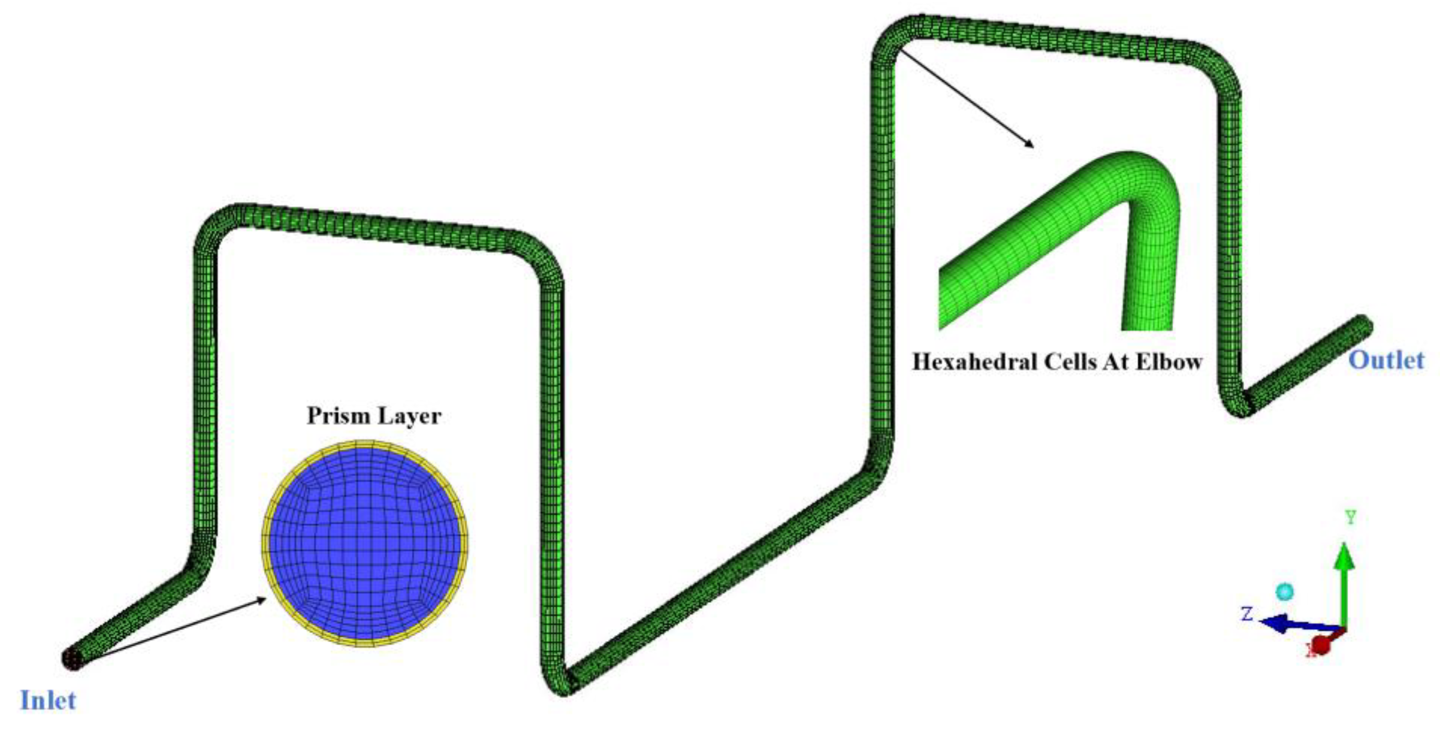
For the numerical simulations of the gas–liquid two-phase flow, the O-grid structured meshes are adopted to discretize the computational domain, as shown in
Figure 4.
Four mesh schemes are set, with grids number ranging from 2.10 × 10
5 to 7.28 × 10
5, as listed in
Table 3. The maximum and minimum total pressure are monitored in section S4 at a liquid superficial velocity
Vsl = 0.5 m/s and a gas superficial velocity
Vsg =1.5 m/s to select the appropriate number of grids. As seen in
Figure 5, the difference between the calculation results of M2 and M3 is insignificant, while the simulation time of M3 is twice as long as M2. Therefore, the grid number M2 selection can already provide sufficient accuracy. The grid resolution of M2 is used to perform all the simulations in the present study, which are performed on a high-performance computer with 40 processors and 32 GB of RAM. A physical time of 5 seconds is run for all the simulations.
4. Experimental Results
For the experiments, it should be mentioned that a sufficiently long acquisition time is chosen for each case so that the statistics, such as the root mean square and averaged values characterizing the vibration and pressure, will not change as time increases.
The pressure fluctuations in section S1 are measured three times under the same working conditions. The spectral data obtained using FFT for the three measurements shown in
Figure 6 display similar distributions. The dominant frequencies and amplitudes of the pressure fluctuations are approximately equal for the three tests, which shows that the experimental results have good repeatability and reliability.
Before the experimental test, the hammering method was used to obtain the natural frequency of the empty jumper (
fie) and water-filled jumper (
fif). The test was conducted by using the multi-point excitation and three-point response method. The response signals of the two acceleration points of the jumper were collected, and FFT of the acceleration decay curve was conducted to obtain the first six natural frequencies, as shown in
Table 4.
4.1. Flow Visualizations
The flow regime map in this paper was employed to distinguish the multiphase flow regime (Kaichirom et al. [
38]), as shown in
Figure 7. Meanwhile, the superficial gas and liquid velocities of the selected experimental cases were extracted from the Kaichiro M flow regime map.
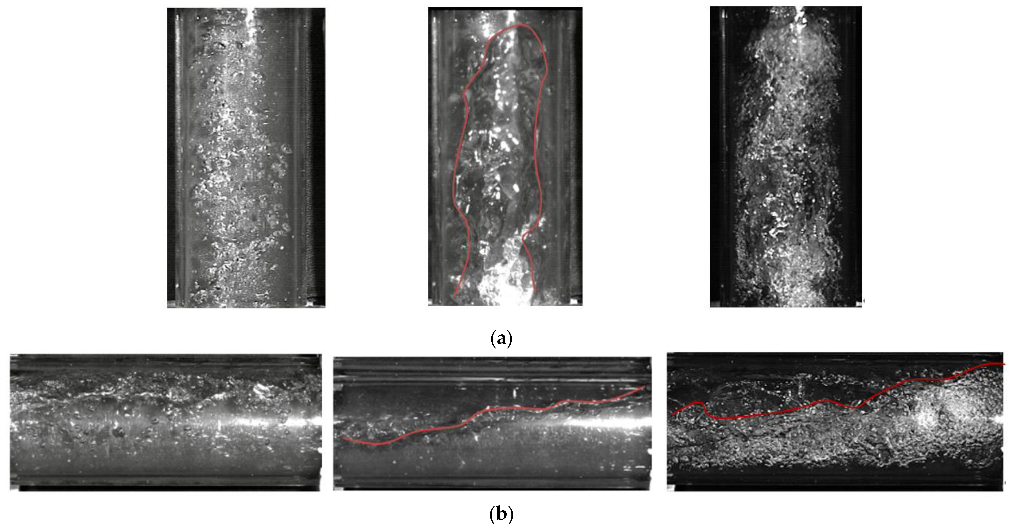
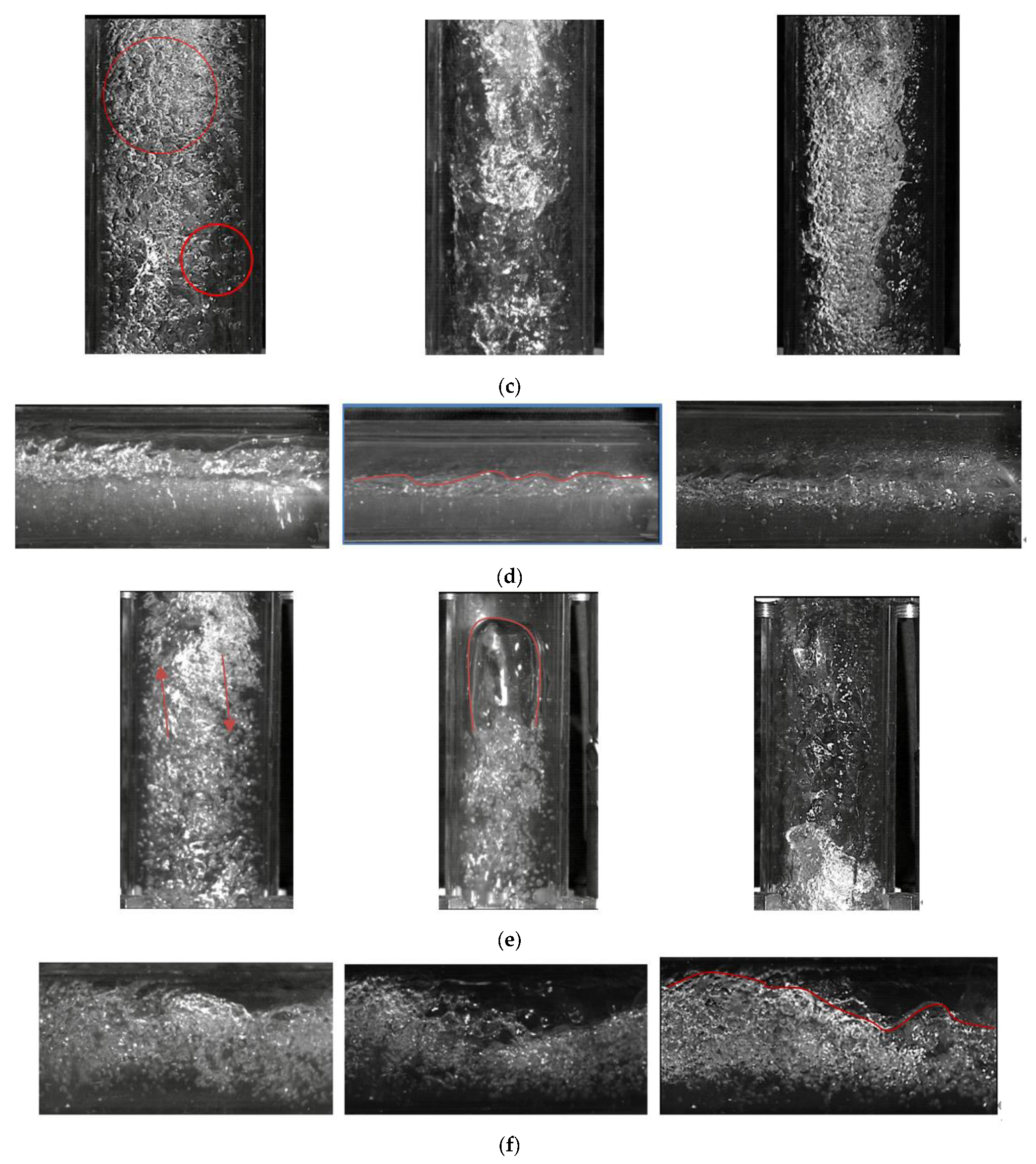
During oil and gas exploration and production periods, the gas rate inside the flow transmission pipeline changes, leading to various flow patterns. A visualization study was carried out for different flow patterns ranging from bubble flow to dispersed annular flow to obtain the flow characteristics and flow pattern transition of the flow inside the jumper. Typical images of the flow visualization are shown in
Figure 8a–f. Multi-level flow pattern transitions are observed in the flow visualization image.
A bubble-dominant flow dominates in the jumper at a low superficial gas–liquid velocity for a
Vsl = 0.8 m/s and
Vsg = 0.5 m/s. The flow pattern of the ascending section S1 taken by the high-speed camera shows that the bubble breaks into smaller groups of bubbles to reach the top of the jumper, as shown in the left column of
Figure 8a. After the bubble flow passes through the first two elbows to the first descending section S3 (as denoted in the left column of
Figure 8c), the bubbles are elongated and split, forming multi-scale bubbles of different sizes and irregular shapes. Before the gas–liquid flow enters the horizontal section S4, the gas–liquid flow goes through the first three elbows and the flow direction changes. Because of the density difference between gas and liquid, the gas-liquid is stratified, where the liquid phase with a high density is in the lower layer and the gas is in the upper layer, and the long horizontal section S4 shows wavy flow, as shown in in the left column of
Figure 8d. In the second ascending section S5, at the low gas flow rate of 0.5 m/s, the flow exists in the form of intermittent bubble flow. The low velocity leads to the entrapment of the liquid phase with air bubbles, and backflow is created under the effect of gravity as denoted in the left column of
Figure 8e. When it reaches Section S6, as shown in the left column of
Figure 8f, more gas is formed than liquid, showing the co-existence of the classical slug flow and bubble flow. At the last descent section S7 (as denoted in the left column of
Figure 8g), the flow pattern becomes churn flow with numerous bubbles.
In the slug-dominant flow for
Vsl = 0.8 m/s and
Vsg = 1.0 m/s, it can be seen that in the first rising section S1 of the jumper, large bullet-shaped bubbles exist in the pipe section as denoted in the middle column of
Figure 8a. The bubbles show the characteristics of a sharp head and a flat tail. This bubble is also called the Taylor bubble, and the bubbles will push the liquid to speed up the upward flow. When reaching the horizontal section S2 in the middle column of
Figure 8b, the liquid phase occupies the main volume, and the flow becomes unstable under the shearing effect of the gas, and the flow state is classified as slug flow. It can be seen that alternate flow exists in the gas–liquid slugs, and there is still gas in the upper part of the liquid slugs. The flow is between the stratified wavy flow and the slug flow. Due to gravity, when it reaches the descending section S3, as shown in the middle column of
Figure 8c, the flow separation of the churn flow appears. The horizontal section S4 appears as a wavy flow, and a stable stratification appears in the flow as denoted in the middle column of
Figure 8d. In the second ascending section S5 (as denoted in the middle column of
Figure 8e), a slug flow with a smaller bubble than that in S1 is formed. In section S6, as shown in the middle column of
Figure 8f, because the gas flow velocity is still low, the liquid surface is unable to cover the whole tube to form a complete liquid plug, and it can be seen that there is still gas in the upper part of the liquid plug. In section S7 (as shown in the middle column of
Figure 8g), the gas–liquid velocity decreases, and a transition to an annular flow can be seen. The flow patterns in the present experiment agree well with those in a U-bent pipeline in Bamidele, et al. [
11].
The churn-dominant flow pattern is more chaotic than the above two cases in the jumper. In the ascending sections S1 and S5 (as shown in the right column of
Figure 8a,e), churn flows of various scales can be seen. In the horizontal sections S2 and S6 (as denoted in the right column of
Figure 8b,f), there are alternating elongated bubble flows and slug flows. In the long horizontal sections S4 (as shown in the right column of
Figure 8d), a gas-dominated stratified flow appears. As the flow passes through the descending sections S3 and S7 (as seen in the right column of
Figure 8c,g), churn and annular flow with droplets is formed.
4.2. Vibration and Pressure Characteristics
The collected acceleration signal generally fluctuates up and down around a certain value. In order to evaluate the intensity of the vibration response at a certain point, the root mean square value of the dynamic fluctuation of acceleration is used to represent the strength of the vibration response, which is defined as follows:
where
aav is the average value of acceleration,
ai is the measured value of acceleration at a certain moment, and
arms is the intensity of vibration response.
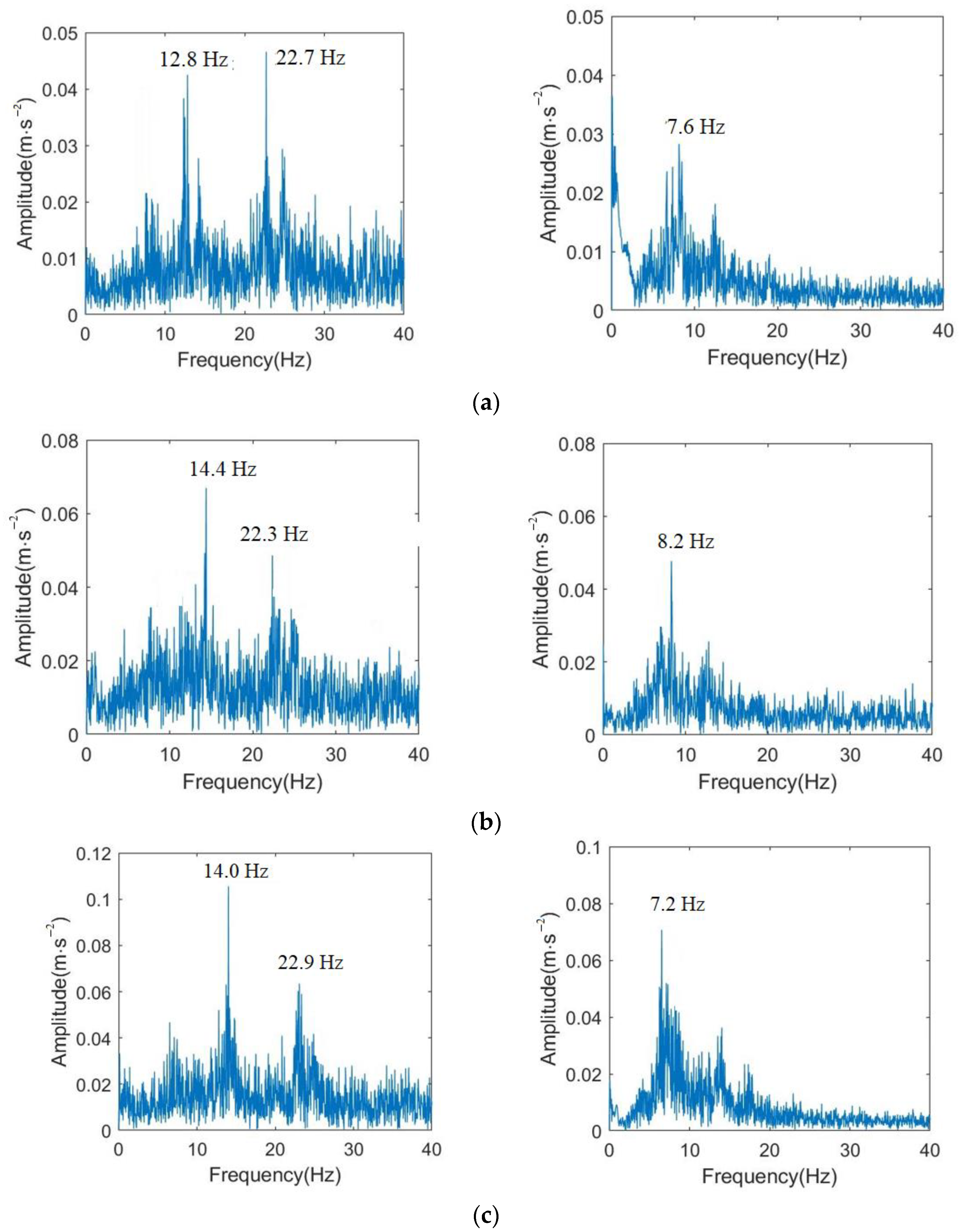
The power spectra densities of the acceleration of the jumper sections of S3 are shown in the left column of
Figure 9, and S7 is denoted in the right column of
Figure 9. It can be found that a number of frequency peaks dominate the spectra at S3 for a
Vsl of 0.8 m/s and a
Vsg of 0.5 m/s, 0.8 m/s, and 2.8 m/s, as shown in the left column of
Figure 9a–c. The dominant frequencies of the modal responses are distributed at approximately 12.8 Hz and 22.9 Hz, which are close to the natural frequency of Modes 3, 4, and 5 as shown in
Table 4. Since section S7 is near the fixed constraint, there is only one frequency peak at approximately 7.6 Hz, which is close to Mode 2.
In the dominant bubble flow in
Figure 9a, the amplitude of acceleration from the vertical axis are the lowest compared with another two cases. When the slug flow dominates, as shown in
Figure 9b, the vibration intensity is stronger than the bubble flow. As shown in
Figure 9c, the dominant churn flow shows that as the mixture of gas–liquid two-phase flow is enhanced, the amplitudes of the jumper vibration also increase correspondingly. In summary, owing to the unsteady gas–liquid two-phase flow, the frequency and amplitude of the dominant vibration modes will change with different flow patterns. The vibration amplitude in the slug flow pattern increases with the superficial velocity of the gas.
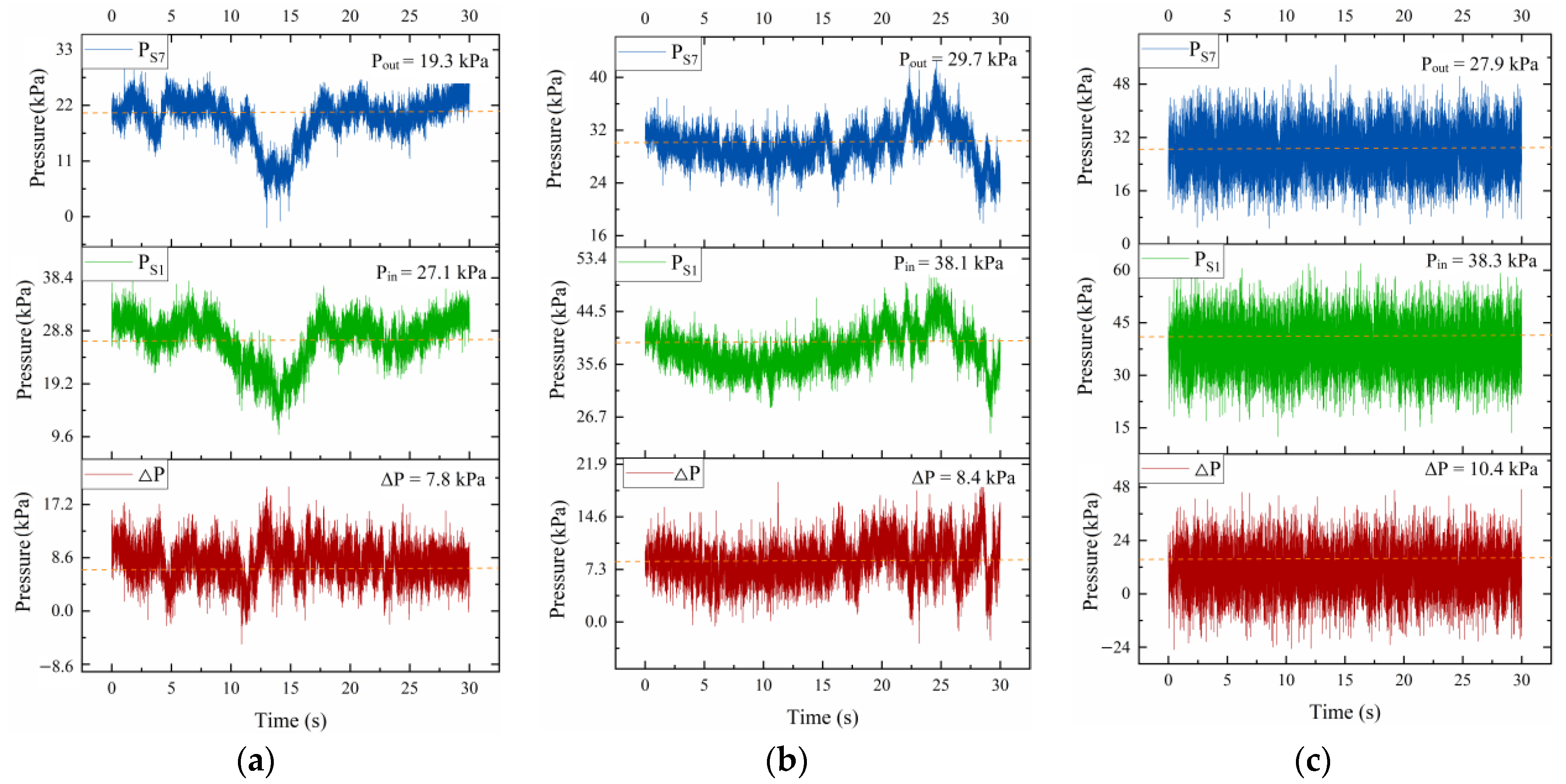
The time signals of the pressures at the inlet and outlet of S1 and S7 for different cases are shown in
Figure 9. After passing through several elbows from the inlet, the average fluid flow pressure gradually decreases. In addition to the pressure drop caused by the gas–liquid and pipe wall effect, the interaction between the two-phase flow also causes a more significant pressure drop. The increase in gas content causes the pressure change curve to flatten out from a curve with a sharp peak.
The inlet and outlet pressure and pressure drop at different volumetric gas content rates, as seen in
Figure 10. In bubble dominant flow in
Figure 10a, the flow pressure drop is the smallest. When the liquid phase flow is more extensive, occupying the main volume, the overall flow in a jumper is more stable. Compared with the churn and other flows, the gas–liquid interaction is small, and the flow pressure drop will be reduced accordingly. Due to the stronger gas perturbation than the liquid phase, the gas–liquid interaction increases, resulting in a more substantial flow pressure drop, as shown in
Figure 10b. The gas-liquid two-phase flow through the jumper has the most significant pressure drop. In the churn-dominant flow in
Figure 10c, the interaction between the gas–liquid flow is more substantial, resulting in the most significant flow pressure drop compared with the other two cases.
4.3. Effect of Two-Phase Flow Characteristics on Vibration and Pressure
The effects of different flow conditions such as the gas content, mixture velocity, superficial flow velocity of the gas–liquid phase on the vibration of the jumper, and the pressure of the two-phase flow in the jumper are investigated. The root mean square (RMS) of the acceleration is used to characterize the vibration response, and the pressure drop is adopted to represent the pressure behavior.
4.3.1. Effect of Void Fraction and Mixing Velocity on Vibration and Pressure
Table 5 shows parameters for different cases to investigate the effects of the void fraction. These include the liquid superficial velocity (
Vsl), the gas superficial velocity (
Vsg), the volumetric gas rate on the inlet (
β), the mass flow rate of the gas phase (
Qmg), and the volumetric flow rate of the liquid phase (
Ql). It can be seen from
Figure 11a that the vibration response intensity is more vigorous when the void fraction is 50% and 75%. It is because the gas–liquid two-phase flow in the jumper is more substantial. Therefore, the pressure drop and the force on the jumper are more significant, as shown in
Figure 11b. At 25% of the void fraction, the interaction between the gas and the liquid phases is weakened, which is reflected in the reduction in the pressure drop and the weakening of the vibration response intensity. At a lower gas content, the flow pattern in the jumper changes to continuous flow, the gas–liquid interaction is small compared with the churn flow, and the flow pressure drop is reduced accordingly.
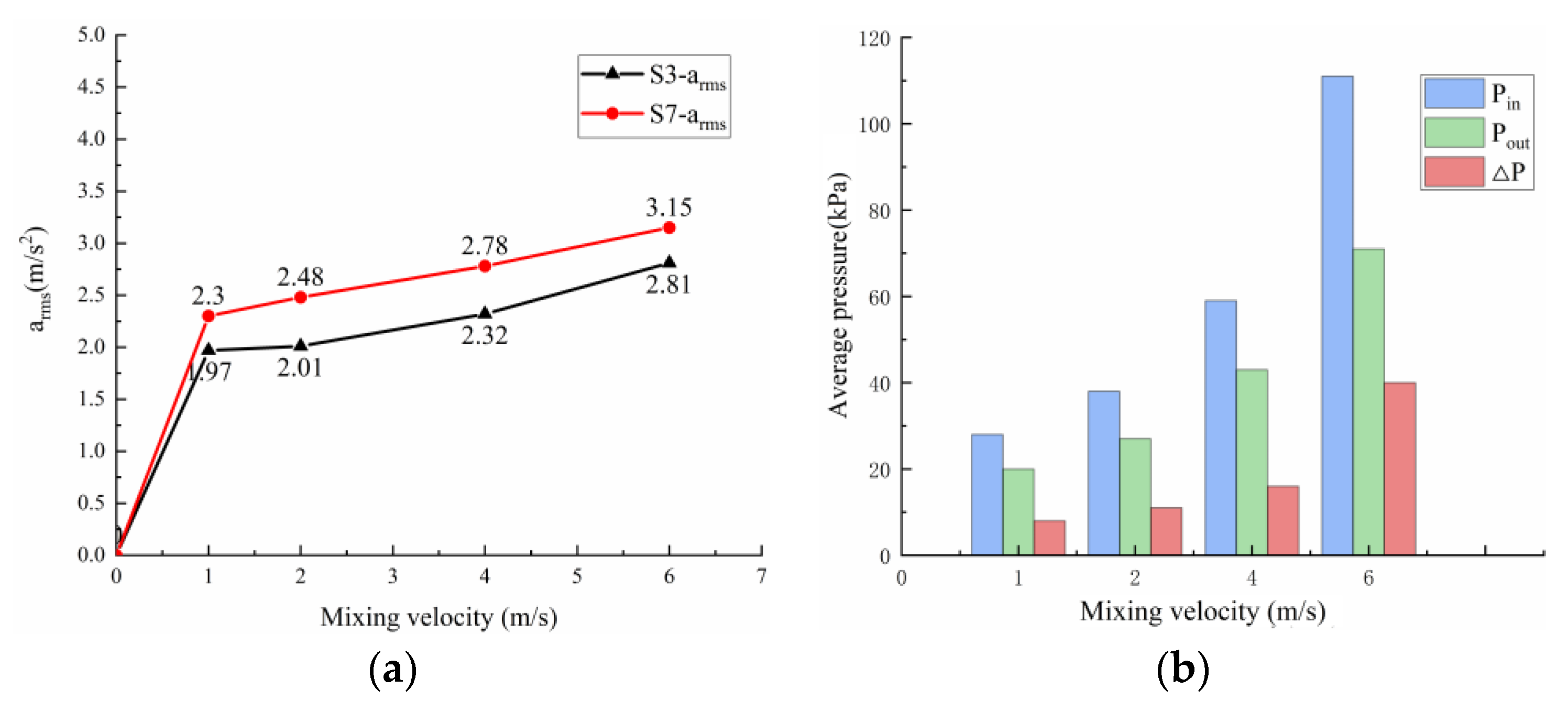
Table 6 shows the parameters of different mixing velocities for the two phases.
Figure 12a shows that the vibration amplitudes increase with the increasing velocity. The mean pressure of the inlet and outlet increases as the mixing speed increases, and the pressure drop between the inlet and outlet also increases as the mixing speed increases, as shown in
Figure 12b. It is because the increasing gas-liquid mixing speed causes a higher resistance along the pipe, which is proportional to the square of the flow rate. As the mixing speed increases, the mixing between gas and liquid becomes intense, and the interaction between the two phases of gas and liquid also increases, resulting in a greater pressure loss.
4.3.2. Effect of Different Liquid/Gas Superficial Velocity on Vibration and Pressure
As the liquid phase flow rate increases, the vibration response becomes more significant, and the vibration intensity gradually increases (see
Figure 13 and
Table 7). As the superficial flow rate of the liquid phase increases, the flow rate of both the gas phase and liquid phase increases. This is because the liquid pressure plays a major role in motivating the gas–liquid flow in the pipe. With the increasing turbulent energy of the liquid, the impact and the mixing between the gas and the liquid becomes more obvious, which further increases the velocities of both the gas and the liquid, and the frictional resistance along the pipe is also larger. Since the friction loss is proportional to the square of the flow rate, an increasing pressure loss is caused. With the increase in the gas phase velocity (see
Table 8), the energy carried by the two-phase flow is larger, which will cause a great impact on the jumper. Thus, the vibration intensity naturally increases. One point that needs to be mentioned is that the gas volume in the jumper is dominant here, while the liquid volume is relatively less, and a negative pressure situation will occur. There is no significant increase in the pressure drop, as shown in
Figure 14. This is because the pressure fluctuation is mainly caused by both the large-scale mixing and the impact within the two-phase flow. Thus, the influences induced by pressure are not obvious if the gas dominates and the flow rate of the liquid is relatively lower in the pipe.
5. Numerical Results and Verifications
5.1. Flow Visualizations
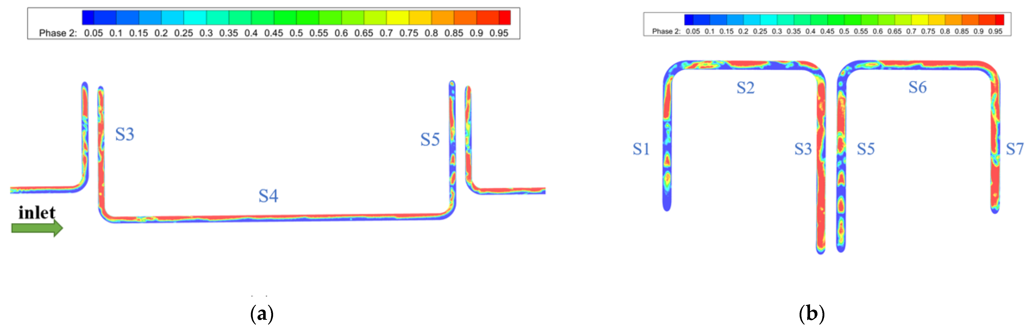
For further validation of the numerical model, computational fluid dynamics simulations are carried out for several groups of working conditions. One of the cases is selected to analyze the flow pattern diagrams obtained from the results and compare them with those obtained from the experimental study. The volume fraction of air is shown in
Figure 15.
A detailed analysis of the flow pattern in each jumper section is also carried out.
Figure 16a shows the flow patterns within the ascending sections S1 and S5, and it can be seen that the liquid phase occupies the main volume in the simulation. A more elongated structure of the gas bullet appears in the liquid phase, which is in good agreement with the experimentally captured flow pattern.
Figure 16b compares the flow patterns in the horizontal sections S2 and S4. It can be seen that the experimental and simulated sections S2 show an apparent slug flow, while the flow pattern in section S4 is a wavy flow with a clear gas–liquid partition interface.
Figure 16c compares the flow patterns in the descending sections S3 and S7. There is gas–liquid separation in section S3, and the liquid phase cannot maintain a regular shape under gravity. The velocity of gas–liquid in section S7 decreases, the liquid is divided by the gas, and the liquid falls on the tube wall as a liquid film, showing an annular flow. It can be shown that the model used in the simulation and the calculation results are qualitatively in good agreement with the actual situation, which validates the numerical model used for gas–liquid two-phase flow.
5.2. Vibration Response
The dynamic response of the jumper is obtained using the one-way transient FSI simulations. The numerical results are validated by comparing them with the present experimental data. As shown in
Figure 17a, the experiment and simulation result in the same average acceleration of 2.8 m/s
2 at the monitoring point of S3 at the liquid superficial velocity (
Vsl) of 1.6 m/s and gas superficial velocity (
Vsg) of 2.0 m/s. The averaged acceleration increases to 4.2 m/s
2 when
Vsl increases to 3.4 m/s, as seen in
Figure 18a. In addition, the PSD plot of the acceleration signature shows narrow band responses for 5.07 Hz (simulation) and 5.31 Hz (experiment) for
Vsl at 1.6 m/s in
Figure 17b, and a greater vibration response is featured when
Vsl increases to 3.4 m/s at 7.24 Hz (simulation) and 7.72 Hz (experiment), as shown in
Figure 18b. Briefly, as the superficial liquid velocity increases, the mean acceleration increases accordingly, indicating that the liquid velocity significantly affects the dynamic response. The results of the vibration response have little error against the simple pipelines, which is attributed to the jumper’s differences in structures and flow conditions. Still, the trend of the time-averaged acceleration and frequency domain response gained in the numerical simulations are in agreement with the experiments.
6. Conclusions
The flow characteristics of gas–liquid two-phase flow and the induced vibration characteristics in a multi-plane jumper were investigated using an experimental system for two-phase flow and flow-induced vibration to analyze the flow patterns and their transitions in different sections. The corresponding vibration responses in a Z-shaped jumper at different gas rates, mixing velocities, and liquid and gas superficial velocities were also obtained and analyzed by comparing the experimental data and the numerical simulation results. The present experiment was conducted according to the practical size of a subsea jumper, and thus can be a benchmark for the design of such a pipeline. Apart from this, it is feasible to employ the present experimental technique and numerical method for the flow-induced vibration characteristics of vertical rising, falling, and horizontal pipelines based on the Reynolds similarity principle. Besides, the analysis method can also be used for oil–gas flow to identify the flow pattern and obtain the pressure characteristics in the rising and horizontal parts. The main conclusions can be summarized as follows:
I. Significant variations in flow patterns were observed in the two-phase flow through the jumper, including dispersed bubbly, slug, churn, wavy, stratified, and annular flows. As the gas content increases, the length of the gas slug in the ascending section S1 increases, the flow in the descending section S3 changes from bubbly to churn flow, and the flow in the horizontal section S4 changes from stratified to wavy flow. On the other hand, with the increasing mixing flow rate, the gas bullet completely breaks into fine bubbles, and the gas–liquid boundary in the S4 section becomes wider with a strong gas–liquid mixture.
II. The vibration characteristics of the jumper are closely related to the flow characteristics of the two-phase flow, especially the flow pattern. When the churn dominates the flow, the intensity of the jumper vibration increases accordingly with the increasing gas–liquid two-phase flow effect. It becomes slug-dominated, and the impact of flow instability is stronger than bubble-dominated flow. While the gas–liquid interaction is weaker, the dynamics of the gas–liquid two-phase flow are closer to that of the single-phase flow.
III. The pressure drop increases significantly when the superficial velocity of the liquid increases, while the trend is not significant when the superficial velocity of the gas phase increases. As the mixing speed increases, the mixing between gas and liquid becomes more and more intense, resulting in larger pressure loss. At a lower gas content, the flow pattern in the jumper changes to continuous flow, and the gas–liquid interaction is smaller, while the flow pressure drop is reduced accordingly.
IV. The one-way transient FSI coupling used in this study is sufficient to predict the dynamic response characteristics of the jumper. The time-averaged accelerations obtained using the finite element method and the flow pattern predicted by using the VOF method under the same conditions are in good agreement with the experimental measurements.
The present study analyzed the two-phase flow and flow-induced vibration of a multi-plane subsea jumper. Only the gas–liquid two-phase was studied and the internal flow effect in the jumper was considered. For future research, a vibration sensor that can measure more dimensions of the vibration response should be adopted for vibration data acquisition and analysis of more parts. In addition to the internal multiphase flow, in a subsea environment, the jumper is also subjected to current flow and undergoes external flow-induced vibration. The coupled vibration characteristics of the jumper under the effects of both internal and external flow need to be investigated in our future studies.
Author Contributions
Conceptualization, W.L., Q.Z., G.Y., M.C.O., G.L. and F.H.; methodology, W.L., Q.Z., G.Y., M.C.O., G.L. and F.H.; software, W.L. and Q.Z.; validation, W.L. and Q.Z.; formal analysis, W.L. and Q.Z.; investigation, W.L., Q.Z., G.L., G.Y. and M.C.O.; data curation, W.L. and Q.Z.; writing—original draft, W.L. and Q.Z.; writing—review and editing, W.L., Q.Z., G.Y., M.C.O., G.L. and F.H.; visualization, W.L. and Q.Z.; resources, W.L.; project administration, W.L.; funding acquisition, W.L. All authors have read and agreed to the published version of the manuscript.
Funding
This research was funded by the Liaoning Provincial Natural Science Foundation of China (2020-HYLH-35), LiaoNing Revitalization Talents Program (XLYC2007092), 111 Project (B18009), the Fundamental Research Funds for the Central Universities (3132022350, 3132022348), the Fundamental Research Funds of National Center for International Research of Subsea Engineering and Equipment (3132022354), and the Cultivation Program for the Excellent Doctoral Dissertation of Dalian Maritime University (2022YBPY002).
Institutional Review Board Statement
Not applicable.
Informed Consent Statement
Not applicable.
Data Availability Statement
Not applicable.
Conflicts of Interest
The authors declare no conflict of interest.
References
- Swindell, R. Hidden integrity threat looms in subsea pipework vibrations. Offshore 2011, 71, 78–81. [Google Scholar]
- Carvalho, F.d.C.T.; Figueiredo, M.d.M.F.; Serpa, A.L. Flow pattern classification in liquid-gas flows using flow-induced vibration. Exp. Therm. Fluid Sci. 2020, 112, 109950. [Google Scholar] [CrossRef]
- Bamidele, O.E.; Hassan, M.; Ahmed, W.H. Flow induced vibration of two-phase flow passing through orifices under slug pattern conditions. J. Fluids Struct. 2021, 101, 103209. [Google Scholar] [CrossRef]
- Orres, L.T.; Noguera, J.; Guzmán-Vázquez, J.E.; Hernández, J.; Sanjuan, M.; Palacio-Pérez, A. Pressure signal analysis for the characterization of high-viscosity two-phase flows in horizontal pipes. J. Mar. Sci. Eng. 2020, 8, 1000. [Google Scholar]
- Xu, H.; Hu, W.C.W. Hydraulic transport flow law of natural gas hydrate pipeline under marine dynamic environment. Eng. Appl. Comput. Fluid Mech. 2020, 14, 507–521. [Google Scholar] [CrossRef]
- Baumann, A.; Hoch, D.; Niessner, J.B.J. Macro-scale modeling and simulation of two-phase flow in fibrous liquid aerosol filters. Eng. Appl. Comput. Fluid Mech. 2020, 14, 1325–1336. [Google Scholar] [CrossRef]
- Dinaryanto, O.; Prayitno, Y.A.K.; Majid, A.I.; Hudaya, A.Z. Experimental investigation on the initiation and flow development of gas-liquid slug two-phase flow in a horizontal pipe. Exp. Therm. Fluid Sci. 2017, 81, 93–108. [Google Scholar] [CrossRef]
- Mohmmed, A.O.; Al-Kayiem, H.H.; Osman, A.B.; Sabir, O. One-way coupled fluid–structure interaction of gas–liquid slug flow in a horizontal pipe: Experiments and simulations. J. Fluids Struct. 2020, 97, 103083. [Google Scholar] [CrossRef]
- Al-Hashimy, Z.I.; Al-Kayiem, H.H.; Time, R.W. Experimental investigation on the vibration induced by slug flow in horizontal pipe. ARPN J. Eng. Appl. Sci. 2016, 11, 20. [Google Scholar]
- Miwa, S.; Hibiki, T.; Mori, M. Analysis of flow-induced vibration due to stratified wavy two-phase flow. J. Fluids Eng. 2016, 138, 091302. [Google Scholar] [CrossRef]
- Bamidele, O.E.; Ahmed, W.H.; Hassan, M. Characterizing two-phase flow-induced vibration in piping structures with u-bends. Int. J. Multiph. Flow 2022, 151, 104042. [Google Scholar] [CrossRef]
- Han, F.; Liu, Y.; Ong, M.C.; Yin, G.; Wang, W.L.Z. Cfd investigation of blind-tee effects on flow mixing mechanism in subsea pipelines. Eng. Appl. Comput. Fluid Mech. 2022, 16, 1395–1419. [Google Scholar] [CrossRef]
- Santos, R.M.; Kawaji, M. Numerical modeling and experimental investigation of gas–liquid slug formation in a microchannel t-junction. Int. J. Multiph. Flow 2010, 36, 314–323. [Google Scholar] [CrossRef]
- Han, F.; Ong, M.C.; Xing, Y.; Li, W. Three-dimensional numerical investigation of laminar flow in blind-tee pipes. Ocean Eng. 2020, 217, 107962. [Google Scholar] [CrossRef]
- Chen, F.; Zhu, G.; Jing, L.; Pan, W.Z.R. Effects of diameter and suction pipe opening position on excavation and suction rescue vehicle for gas-liquid two-phase position. Eng. Appl. Comput. Fluid Mech. 2020, 14, 1128–1155. [Google Scholar] [CrossRef]
- Rouhani, S.Z.; Sohal, M.S. Two-phase flow patterns: A review of research results. Prog. Nucl. Energ. 1983, 11, 219–259. [Google Scholar] [CrossRef]
- Bruschi, R.; Parrella, A.; Vignati, G.C.; Vitali, L. Crucial issues for deep water rigid jumper design. Ocean Eng. 2017, 137, 193–2003. [Google Scholar] [CrossRef]
- Li, L.; Zhu, X.; Parra, C.; Ong, M.C. Comparative study on two deployment methods for large subsea spools. Ocean Eng. 2021, 233, 109202. [Google Scholar] [CrossRef]
- Qu, Y.; Fu, S.; Liu, Z.; Xu, Y.; Sun, J. Numerical study on the characteristics of vortex-induced vibrations of a small-scale subsea jumper using a wake oscillator model. Ocean Eng. 2022, 243, 110028. [Google Scholar] [CrossRef]
- Ren, H.; Zhang, M.; Cheng, J.; Cao, P.; Xu, Y.; Fu, S.; Liu, C. Experimental investigation on vortex-induced vibration of a flexible pipe under higher mode in an oscillatory flow. J. Mar. Sci. Eng. 2020, 8, 408. [Google Scholar] [CrossRef]
- Cheng, P.; Zhang, J.; Gui, N.; Yang, X.; Jiang, J.T.S. Numerical investigation of two-phase flow through tube bundles based on the lattice boltzmann method. Eng. Appl. Comput. Fluid Mech. 2022, 16, 1233–1263. [Google Scholar] [CrossRef]
- Wang, J.; Chen, F.; Shi, C.; Yu, J. Mitigation of vortex-induced vibration of cylinders using cactus-shaped cross sections in subcritical flow. J. Mar. Sci. Eng. 2021, 9, 292. [Google Scholar] [CrossRef]
- Holmes, S.; Constantinides, Y. Vortex induced vibration analysis of a complex subsea jumper. In Proceedings of the ASME 2010 29th International Conference on Ocean, Offshore and Arctic Engineering, Shanghai, China, 6–11 June 2010. [Google Scholar]
- Zhu, H.; Gao, Y.; Zhao, H. Experimental investigation of slug flow-induced vibration of a flexible riser. Ocean Eng. 2019, 189, 106370. [Google Scholar] [CrossRef]
- Jujuly, M.M.; Rahman, M.; Maynard, A.; Adey, M. Hydrate-induced vibration in an offshore pipeline. In Proceedings of the SPE Annual Technical Conference and Exhibition, San Antonio, TX, USA, 9–11 October 2017. [Google Scholar]
- Talley, J.D.; Worosz, T.; Kim, S.; Buchanan, J.R., Jr. Characterization of horizontal air–water two-phase flow in a round pipe part I: Flow visualization. Int. J. Multiph. Flow 2015, 76, 212–222. [Google Scholar] [CrossRef]
- Chica, L.; Pascali, R.; Jukes, P.; Ozturk, B.; Gamino, M.; Smith, K. Detailed fsi analysis methodology for subsea piping components. In Proceedings of the ASME 2012 31st International Conference on Ocean, Offshore and Arctic Engineering, Rio de Janeiro, Brazil, 1–6 July 2012. [Google Scholar]
- Elyyan, M.A.; Perng, Y.-Y.; Doan, M. Fluid-structure interaction modeling of subsea jumper pipe. In Proceedings of the ASME 2014 33rd International Conference on Ocean, Offshore and Arctic Engineering, San Francisco, CA, USA, 8–13 June 2014. [Google Scholar]
- Chen, Y.; Zhang, H.; Zhang, J.; Li, X.; Zhou, J. Failure analysis of high strength pipeline with single and multiple corrosions. Mater. Des. 2014, 10, 088. [Google Scholar] [CrossRef]
- Wang, J.; Sawant, S.; Wang, F.S.; Jukes, T.N.A.P. Analysis of jumpers subject to various loading conditions. In Proceedings of the Twenty-First (2011) International Offshore and Polar Engineering Conference, Maui, HI, USA, 19–24 July 2011. [Google Scholar]
- Dai, Y.; Liu, Z.; Zhang, W.; Chen, J.; Liu, J. Cfd-fem analysis of flow-induced vibrations in waterjet propulsion unit. J. Mar. Sci. Eng. 2022, 10, 1032. [Google Scholar] [CrossRef]
- Lu, Y.; Liang, C.; Manzano-Ruiz, J.J.; Janardhanan, K.; Perng, Y.-Y. Flow-induced vibration in subsea jumper subject to downstream slug and ocean current. J. Offshore Mech. Arct. Eng. 2016, 138, 021302. [Google Scholar] [CrossRef]
- Song, M.; Gheroufella, M.; Chartier, P. Machine learning prediction and reliability analysis applied to subsea spool and jumper design. In Proceedings of the ASME 2021 40th International Conference on Ocean, Offshore and Arctic Engineering, Online, 21–30 June 2021. [Google Scholar]
- Nair, A.; Chauvet, C.; Whooley, A.; Eltaher, A.; Jukes, P. Flow induced forces on multi-planar rigid jumper systems. In Proceedings of the ASME 2011 30th International Conference on Ocean, Offshore and Arctic Engineering, Rotterdam, The Netherlands, 19–24 June 2011. [Google Scholar]
- Pontaza, J.P.; Menon, R.G. Flow-induced vibrations of subsea jumpers due to internal multi-phase flow. In Proceedings of the ASME 2011 30th International Conference on Ocean, Offshore and Arctic Engineering, Rotterdam, The Netherlands, 19–24 June 2011. [Google Scholar]
- Liu, S.; Ong, M.C.; Obhrai, C. Numerical simulations of breaking waves and steep waves past a vertical cylinder at different keulegan–carpenter numbers. J. Offshore Mech. Arct. Eng. 2019, 141, 041806. [Google Scholar] [CrossRef]
- Wilcox, D.C. Formulation of the k-ω turbulence model revisited. AIAA J. 2008, 46, 11. [Google Scholar] [CrossRef]
- Mishima, K.; Ishii, M. Flow regime transition criteria for upward two-phase flow in vertical tubes. Int. J. Heat Mass Tran. 1984, 27, 723–737. [Google Scholar]
Figure 1.
Flow regimes: (
a) Vertical pipes for up-flow (
b) horizontal pipes [
16]. (Reproduced with permission from Rouhani, S.Z.; M.S. Sohal, Two-phase flow patterns: A review of research results, published by Pergamon Press Ltd., Oxford, UK, 1983).
Figure 1.
Flow regimes: (
a) Vertical pipes for up-flow (
b) horizontal pipes [
16]. (Reproduced with permission from Rouhani, S.Z.; M.S. Sohal, Two-phase flow patterns: A review of research results, published by Pergamon Press Ltd., Oxford, UK, 1983).
Figure 2.
The experimental setup: (a) Experimental facility setup. (b) The diagram of the two-phase flow loop. 1: Air compressor; 2: Air bottle; 3: Freeze dryer; 4: Water pump; 5: Three-phase separator; 6: Transparent visualization window; 7: High-speed camera; 8: Shut-off valve; 9: Pneumatic ball valve; 10: Filter; 11: Pressure sensor; 12: Vibration sensor; 13: Temperature sensor; and 14: Flow sensor.
Figure 3.
The test section of the Z-shaped jumper: (a) The Z-shaped jumper model; (b) detailed jumper model and global coordinate system.
Figure 3.
The test section of the Z-shaped jumper: (a) The Z-shaped jumper model; (b) detailed jumper model and global coordinate system.
Figure 4.
Detailed mesh of the jumper.
Figure 4.
Detailed mesh of the jumper.
Figure 5.
The total pressure at specific monitoring points for four mesh sizes: (a) The minimum total pressures; (b) the maximum total pressures.
Figure 5.
The total pressure at specific monitoring points for four mesh sizes: (a) The minimum total pressures; (b) the maximum total pressures.
Figure 6.
Repeatability validation.
Figure 6.
Repeatability validation.
Figure 7.
Flow regime maps based on Mishima and Ishii [
38]. (Reproduced with permission from MISHIMA, K.; ISHII, M, Flow regime transition criteria for upward two-phase flow in vertical tubes, published by Pergamon Press Ltd., Oxford, UK, 1984).
Figure 7.
Flow regime maps based on Mishima and Ishii [
38]. (Reproduced with permission from MISHIMA, K.; ISHII, M, Flow regime transition criteria for upward two-phase flow in vertical tubes, published by Pergamon Press Ltd., Oxford, UK, 1984).
Figure 8.
Flow visualization for bubbly (left), slug (middle), and churn (right) flows showing the flow regime transition in the Z-shaped jumper: (a) S1, (b) S2, (c) S3, (d) S4, (e) S5, (f) S6, and (g) S7 for a Vsl = 0.8 m/s, and Vsg is 0.5 m/s (left), 1.0 m/s (middle), and 2.8 m/s (right).
Figure 8.
Flow visualization for bubbly (left), slug (middle), and churn (right) flows showing the flow regime transition in the Z-shaped jumper: (a) S1, (b) S2, (c) S3, (d) S4, (e) S5, (f) S6, and (g) S7 for a Vsl = 0.8 m/s, and Vsg is 0.5 m/s (left), 1.0 m/s (middle), and 2.8 m/s (right).
Figure 9.
The PSD of jumper acceleration amplitude in S3 (left) and S7 (right) with the frequency for Vsl = 0.8 m/s and Vsg is (a) 0.5 m/s, (b) 1.0 m/s, and (c) 2.8 m/s.
Figure 9.
The PSD of jumper acceleration amplitude in S3 (left) and S7 (right) with the frequency for Vsl = 0.8 m/s and Vsg is (a) 0.5 m/s, (b) 1.0 m/s, and (c) 2.8 m/s.
Figure 10.
Plot of jumper average inlet and outlet pressure and pressure drop for Vsl = 0.8 m/s and Vsg is (a) 0.5 m/s, (b) 1.0 m/s, and (c) 2.8 m/s.
Figure 10.
Plot of jumper average inlet and outlet pressure and pressure drop for Vsl = 0.8 m/s and Vsg is (a) 0.5 m/s, (b) 1.0 m/s, and (c) 2.8 m/s.
Figure 11.
Effect of void fraction on two-phase flow: (a) The RMS of the vibration acceleration and (b) pressure drop.
Figure 11.
Effect of void fraction on two-phase flow: (a) The RMS of the vibration acceleration and (b) pressure drop.
Figure 12.
Effect of mixing velocity on two-phase flow: (a) The RMS of the vibration acceleration and (b) pressure drop.
Figure 12.
Effect of mixing velocity on two-phase flow: (a) The RMS of the vibration acceleration and (b) pressure drop.
Figure 13.
Effect of liquid superficial velocity on two-phase flow: (a) The RMS of the vibration acceleration and (b) pressure drop.
Figure 13.
Effect of liquid superficial velocity on two-phase flow: (a) The RMS of the vibration acceleration and (b) pressure drop.
Figure 14.
Effect of gas superficial velocity on two-phase flow: (a) The RMS of the vibration acceleration and (b) pressure drop.
Figure 14.
Effect of gas superficial velocity on two-phase flow: (a) The RMS of the vibration acceleration and (b) pressure drop.
Figure 15.
The slug-dominant flow morphology of CFD simulation for a Vsl = 0.8 m/s, Vsg = 1.0 m/s: (a) Front-view; (b) left-view.
Figure 15.
The slug-dominant flow morphology of CFD simulation for a Vsl = 0.8 m/s, Vsg = 1.0 m/s: (a) Front-view; (b) left-view.
Figure 16.
Comparison of detail section flow patterns in (a) rising sections S1 and S5, (b) horizontal sections S2 and S4, (c) descending sections S3 and S7 for Vsl = 0.8 m/s, Vsg = 1.0 m/s.
Figure 16.
Comparison of detail section flow patterns in (a) rising sections S1 and S5, (b) horizontal sections S2 and S4, (c) descending sections S3 and S7 for Vsl = 0.8 m/s, Vsg = 1.0 m/s.
Figure 17.
Comparison between the acceleration amplitude results from the FSI simulation and experimental measurements for a Vsl = 1.6 m/s, Vsg = 2.0 m/s: (a) Time domain diagram of acceleration; (b) the corresponding PSD of acceleration.
Figure 17.
Comparison between the acceleration amplitude results from the FSI simulation and experimental measurements for a Vsl = 1.6 m/s, Vsg = 2.0 m/s: (a) Time domain diagram of acceleration; (b) the corresponding PSD of acceleration.
Figure 18.
Comparison between the acceleration amplitude results from the FSI simulation and experimental measurements for a Vsl = 3.4 m/s, Vsg = 2.0 m/s: (a) Time domain diagram of acceleration; (b) the corresponding PSD of acceleration.
Figure 18.
Comparison between the acceleration amplitude results from the FSI simulation and experimental measurements for a Vsl = 3.4 m/s, Vsg = 2.0 m/s: (a) Time domain diagram of acceleration; (b) the corresponding PSD of acceleration.
Table 1.
Parameters of the jumper model.
Table 1.
Parameters of the jumper model.
| Parameter | Values | Dimension |
|---|
| Total length | 3.4 | m |
| Outer diameter | 0.052 | m |
| Inner diameter | 0.048 | m |
| Wall thickness | 0.002 | m |
| Transparent section length | 0.23 | m |
| S1, S2, S6, S7 | 0.5 | m |
| S3, S5 | 0.8 | m |
| S4 | 2 | m |
| Density | 7850 | kg/m3 |
| Poisson’s ratio | 0.3 | |
| Young’s Modulus | 2.06 × 10⁵ | MPa |
Table 2.
Physical properties of the fluid.
Table 2.
Physical properties of the fluid.
ρg
(kg/m3) | μg
(kg/m·s) | ρl
(kg/m3) | μl
(kg/m·s) | Surface Tension
(N/m) |
|---|
| 1.29 | 1.8 × 10⁻⁵ | 998.2 | 1.0 × 10⁻³ | 0.072 |
Table 3.
The total pressures for the different numbers of grids.
Table 3.
The total pressures for the different numbers of grids.
| Mesh | Grids Number | The Min Pressure (Pa) | The Max Pressure (Pa) |
|---|
| M1 | 2.10 × 10⁵ | 3.92 × 10³ | 2.01 × 10⁴ |
| M2 | 3.49 × 10⁵ | 2.48 × 10³ | 2.58 × 10⁴ |
| M3 | 6.05 × 10⁵ | 2.07 × 10³ | 2.78 × 10⁴ |
| M4 | 7.28 × 10⁵ | 2.26 × 10³ | 2.68 × 10⁴ |
Table 4.
The first six natural frequencies were obtained with the water-filled and empty jumpers.
Table 4.
The first six natural frequencies were obtained with the water-filled and empty jumpers.
| Mode | fie (Hz) | fif (Hz) |
|---|
| 1 | 4.98 | 4.09 |
| 2 | 6.31 | 7.23 |
| 3 | 12.42 | 13.52 |
| 4 | 15.03 | 15.47 |
| 5 | 22.43 | 23.67 |
| 6 | 23.82 | 31.33 |
Table 5.
The case parameters for parametric studies of void fraction.
Table 5.
The case parameters for parametric studies of void fraction.
Case
No. | Vsg
(m/s) | Vsl
(m/s) | β | Qmg
(kg/h) | Ql
(t/h) |
|---|
| 1 | 0.5 | 1.5 | 0.25 | 4.2 | 9.75 |
| 2 | 1 | 1 | 0.5 | 8.4 | 6.5 |
| 3 | 1.5 | 0.5 | 0.75 | 12.6 | 3.25 |
Table 6.
The case parameters for parametric studies of reduced velocity.
Table 6.
The case parameters for parametric studies of reduced velocity.
Case
No. | Vsg
(m/s) | Vsl
(m/s) | β | Qmg
(kg/h) | Ql
(t/h) |
|---|
| 4 | 0.5 | 0.5 | 0.5 | 4.2 | 3.25 |
| 5 | 1 | 1 | 0.5 | 8.4 | 6.5 |
| 6 | 2 | 2 | 0.5 | 16.8 | 13 |
| 7 | 3 | 3 | 0.5 | 25.2 | 19.5 |
Table 7.
The case parameters for parametric studies of the liquid superficial velocity.
Table 7.
The case parameters for parametric studies of the liquid superficial velocity.
Case
No. | Vsg
(m/s) | Vsl
(m/s) | β | Qmg
(kg/h) | Ql
(t/h) |
|---|
| 8 | 2 | 0.7 | 0.74 | 16.8 | 4.55 |
| 9 | 2 | 1.6 | 0.56 | 16.8 | 10.4 |
| 10 | 2 | 2.1 | 0.48 | 16.8 | 13.65 |
| 11 | 2 | 3.2 | 0.38 | 16.8 | 20.8 |
Table 8.
The case parameters for parametric studies of the gas superficial velocity.
Table 8.
The case parameters for parametric studies of the gas superficial velocity.
Case
No. | Vsg
(m/s) | Vsl
(m/s) | β | Qmg
(kg/h) | Ql
(t/h) |
|---|
| 12 | 0.5 | 0.8 | 0.38 | 4.2 | 5.2 |
| 13 | 1.0 | 0.8 | 0.56 | 8.4 | 5.2 |
| 14 | 2.1 | 0.8 | 0.72 | 17.64 | 5.2 |
| 15 | 2.8 | 0.8 | 0.78 | 23.52 | 5.2 |
| Publisher’s Note: MDPI stays neutral with regard to jurisdictional claims in published maps and institutional affiliations. |
© 2022 by the authors. Licensee MDPI, Basel, Switzerland. This article is an open access article distributed under the terms and conditions of the Creative Commons Attribution (CC BY) license (https://creativecommons.org/licenses/by/4.0/).


